The Balance‐Sample Size Frontier in Matching Methods for ...

The Balance-Sample Size Frontier in MatchingMethods for Causal Inference∗
Gary King† Christopher Lucas‡ Richard Nielsen§
February 28, 2015
Abstract
We propose a simplified approach to matching for causal inference that simultane-ously optimizes both balance (between the treated and control groups) and matchedsample size. This procedure resolves two widespread tensions in the use of this pop-ular methodology. First, current practice is to run a matching method that maximizesone balance metric (such as a propensity score or average Mahalanobis distance), butthen to check whether it succeeds with respect to a different balance metric for whichit was not designed (such as differences in means or L1). Second, current match-ing methods either fix the sample size and maximize balance (e.g., Mahalanobis orpropensity score matching), fix balance and maximize the sample size (such as coars-ened exact matching), or are arbitrary compromises between the two (such as caliperswith ad hoc thresholds applied to other methods). These tensions lead researchers toeither try to optimize manually, by iteratively tweaking their matching method andrechecking balance, or settle for suboptimal solutions. We address these tensions byfirst defining and showing how to calculate the matching frontier as the set of match-ing solutions with maximum balance for each possible sample size. Researchers canthen choose one, several, or all matching solutions from the frontier for analysis inone step without iteration. The main difficulty in this strategy is that checking allpossible solutions is exponentially difficult. We solve this problem with new algo-rithms that finish fast, optimally, and without iteration or manual tweaking. We alsooffer easy-to-use software that implements these ideas, along with analyses of theeffect of sex on judging and job training programs that show how the methods weintroduce enable us to extract new knowledge from existing data sets.
∗Our thanks to Carter Coberley, Stefano Iacus, Walter Mebane, Giuseppe Porro, Molly Roberts, RocioTitiunik, Aaron Wells, and Yu Xie. Jeff Lewis’ comments on an early version were especially helpful.Software to implement the ideas in this can be found at http://projects.iq.harvard.edu/frontier†Albert J. Weatherhead III University Professor, Institute for Quantitative Social Science, 1737 Cam-
bridge Street, Harvard University, Cambridge MA 02138; GaryKing.org, [email protected], (617) 500-7570.‡Ph.D. Candidate, Institute for Quantitative Social Science, 1737 Cambridge Street, Harvard University,
Cambridge MA 02138; christopherlucas.org, [email protected], (617) 982-2718.§Assistant Professor, Massachusetts Institute of Technology, 77 Massachusetts Ave, Cambridge MA
02139; www.mit.edu/∼rnielsen, [email protected], (857) 998-8039.
1

1 IntroductionMatching has attained popularity among applied researchers as a statistically powerful
and conceptually simple method of improving causal inferences in observational data
analysis. It is especially simple in applied statistics when thought of as a nonparamet-
ric preprocessing step that identifies data subsets from which causal inferences can be
drawn with greatly reduced levels of model dependence (Ho et al., 2007). Although suc-
cessful applications of matching require both reduced imbalance (between the treated and
control groups) and a sufficiently large matched sample, existing matching methods op-
timize with respect to only one of these two factors, with the required joint optimization
performed by manually tweaking existing methods or ignored altogether. This is crucial
since, if the subset identified by the matching method is too small, the reduction in model
dependence (and hence bias) achieved will be counterbalanced by an unacceptably high
variance. Similarly, the small variance associated with a large matched data subset may be
counterbalanced by unacceptably high levels of imbalance (and thus model dependence
and bias). Some of this problem may also be induced by current matching methods, which
optimize with respect to one balance metric but cause researchers using them to check the
level of balance achieved with respect to a different metric for which the method was not
designed and does not optimize.
To remedy these problems, we introduce a procedure that enables researchers to de-
fine, estimate, visualize, and then choose from what we call the matching frontier, which
fully characterizes the trade-off between imbalance (with a user-chosen metric) and the
matched sample size. Unlike other approaches, we allow researchers to evaluate how
much balance is achieved by pruning observations and simultaneously trade this off against
the lower variance produced by larger matched sample sizes. At each location (denoted
by the matched sample size) along the matching frontier, our approach offers a matched
subset of the complete data such that no other possible subsets of the same size has lower
imbalance. Any matching solution not on this frontier is suboptimal, in that a lower
level of imbalance can be achieved for the same size data subset. This means that no
matching method can outperform this approach, given a choice of imbalance metric. In
2

this sense, our approach achieves all of the benefits of any individual matching method,
allows researchers to extract maximal causal information from their observational data,
avoids many of the pitfalls and difficulties that lead researchers to ignore best practices
in applications, is considerably easier to apply appropriately, and can reveal considerably
more information about the data.
We begin by introducing the trade-off in matching between pruning observations to
reduce model dependence and retaining observations to reduce variance (Section 2). We
then detail our mathematical notation, goals, and assumptions (Section 3), the choices
required for defining a matching frontier (Section 4), and a formal definition of and algo-
rithms for calculating the frontier (Section 5). Finally, we offer several empirical examples
(Section 6) and conclude (Section 7). Software to implement all the ideas in this paper
can be found at http://projects.iq.harvard.edu/frontier (King, Lucas
and Nielsen, 2015).
2 The Matching Frontier Trade-offMatching methods selectively prune observations from a data set to reduce imbalance. A
reduction in imbalance reduces, or reduces the bound on, the degree of model dependence,
a result which has been shown both formally (King and Zeng, 2006; Imai, King and Stuart,
2008; Iacus, King and Porro, 2011a) and in real data (Ho et al., 2007). However, matching
has a potential cost in that observations pruned from the data may increase the variance
of the causal effect estimate. Although researchers using matching confront the same
bias-variance trade-off as in most of statistics, two issues prevent one from optimizing
on this scale directly. First, since matching is commonly treated as a preprocessing step,
rather than a statistical estimator, particular points on the bias-variance frontier cannot be
computed without also simultaneously evaluating the estimation procedure applied to the
resulting matched data set. Second, best practice in matching involves avoiding selection
bias by ignoring the outcome variable while matching (Rubin, 2008), the consequence of
which is that we give up the ability to control either bias or variance directly.
Thus, instead of bias, matching researchers focus on reducing the closely related quan-
tity, imbalance. The specific mathematical relationship between the two is given by Imai,
3

King and Stuart (2008) but conceptually, imbalance along with the relative importance of
individual covariates determines bias. Researchers exclude relative importance because
it cannot be estimated without the outcome variable (although scaling the covariates by
prior expectations of importance is a common and valuable step). Similarly, instead of
variance, researchers focus on the matched sample size. The variance is determined by
the matched sample size along with the heterogeneity (i.e., residual unit-level variance) in
the data. Researchers exclude heterogeneity because it can only be estimated by using the
outcome variable.
Thus, the goal of matching involves the joint optimization of imbalance and matched
sample size. Optimizing with respect to one, but not both, would be a mistake. Existing
methods address the joint optimization by combining machine optimization of one of
these factors with manual (human) optimization of the other. Of course, it is easy to see
that optimizing by hand in this way is time consuming and usually produces results which
are suboptimal.
Many good suggestions for ad hoc approaches to manual optimization of matching
methods have appeared in the methodological literature (e.g., Austin, 2008; Caliendo and
Kopeinig, 2008; Rosenbaum, Ross and Silber, 2007; Stuart, 2008). For example, Rosen-
baum and Rubin (1984) detail their gradual refinement of an initial model by including
and excluding covariates until they obtain a final model with 45 covariates, including 7
interaction degrees of freedom and 1 quadratic term. Ho et al. (2007, p.216) recommend
trying as many matching solutions as possible and choosing the one with the best bal-
ance. Imbens and Rubin (2009) propose running propensity score matching, checking
imbalance, adjusting the specification, and iterating until convergence, as well as manual
adjustments. Applying most of these methods can be inconvenient, difficult to use op-
timally, and hard to replicate. With nearest neighbor and propensity score matching in
particular, tweaking the procedure to improve imbalance with respect to one variable will
often make it worse on others, and so the iterative process can be frustrating to apply in
practice.
Because of these issues, following suggested best practices, such as these, in applied
4

literatures is rare. In what follows, we replace a machine-human optimization proce-
dure with a machine-machine optimization procedure, thus guaranteeing optimal results
in considerably less time.
3 Causal Inference ObjectivesWe define here our notation (Section 3.1) and choices for the causal quantity of interest
(Section 3.2). We separate discussion of the necessary assumptions into those which are
logically part of the notation and, in Section 3.3, assumptions which become necessary
when trying to learn about the quantities of interest from the data.
3.1 Notation and Basic Assumptions
For unit i, let Ti denote a treatment variable coded 1 for units in the treated group and
0 in the control group. Let Yi(t) (for t = 0, 1) be the (potential) value the outcome
variable would take if Ti = t. Denote the treatment effect of T on Y for unit i as TEi =
Yi(1)−Yi(0). However, for each i, either Yi(1) or Yi(0) is observed, but never both (which
is known as the fundamental problem of causal inference; Holland 1986). This means we
observe Yi = TiYi(1) + (1− Ti)Yi(0). Finally, define a vector of k pre-treatment control
variables Xi.
We simplify this general framework by restricting ourselves to studies or functions of
TEs only for treated units. (Since the definition of which group is labeled treated is arbi-
trary, this does not restrict us much in practice.) In this situation, the only unobservables
are Yi(0) for units which received treatment Ti = 1 (since Yi(1) ≡ Yi is observed for these
units).
A coherent interpretation of this notation implies two assumptions (Imbens, 2004).
First, is overlap (sometimes called “common support”): Pr(Ti = 1|X) < 1 for all i (see
also Heckman, Ichimura and Todd, 1998, p.263). The idea here is that for treated units,
where Ti = 1, it must be conceivable that before treatment assignment an intervention
could have taken place that would have assigned unit i instead to the control group, while
holding constant the values of X . If this could not have been possible, then Yi(0), which
we need to define TEi, does not even logically exist.
A second assumption implied by the notation is stable unit treatment value (SUTVA),
5

which can be thought of as logical consistency, so that each potential value is fixed even if
T changes (or conceptualized differently, no interference and no versions of treatments)
(VanderWeele and Hernan, 2012). As an example that would violate this assumption,
suppose Yi(0) = 5 in the actual case for this treated unit where Ti = 1, but Yi(0) = 8
in the counterfactual condition if this same unit had instead been assigned to the control
group. If overlap holds but SUTVA does not, then Yi(0) and TEi exist but are not fixed
quantities to be estimated.
3.2 Quantities of Interest
From the basic definitions in Section 3.1, we can compute many quantities, based on
the average of TE over given subsets of units. We focus on two in this paper. We first
define these theoretically and then explain how they work in practice, followed by the
assumptions necessary for identification.
First is the sample average treatment effect on the treated, SATT = meani∈{T=1}(TEi),
which is TE averaged over the set of all treated units {T = 1} (Imbens, 2004). (Formally,
for set S with cardinality #S, define the average over i of function g(i) as meani∈S[g(i)] =
1#S
∑#Si=1 g(i).) If matching only prunes data from the control group, SATT is fixed
throughout the analysis.
Second, since many real observational data sets contain some treated units without
good matches, analysts often choose to compute a causal effect among only those treated
observations for which good matches exist. We designate this as the feasible sample
average treatment effect on the treated or FSATT.1 Other possibilities include TE averaged
over all observations, population average treatment effects, among others.
Although the distinction between SATT and FSATT is clear given a data set, the dis-1Using FSATT is common in the matching literature but may be seen as unusual elsewhere in that the
quantity of interest is defined by the statistical procedure, but in fact it follows the usual practice in obser-vational data analysis of collecting data and making inferences only where it is possible to learn something.The advantage here is that the methodology makes a contribution to a step previously considered outside thestatistical framework (e.g., Crump et al., 2009; Iacus, King and Porro, 2011a), just as measurement error,missing data, selection bias, and other issues once were. As Rubin (2010, p.1993) puts it, “In many cases,this search for balance will reveal that there are members of each treatment arm who are so unlike anymember of the other treatment arm that they cannot serve as points of comparison for the two treatments.This is often the rule rather than the exception, and then such units must be discarded. . . . Discarding suchunits is the correct choice: A general answer whose estimated precision is high, but whose validity rests onunwarranted and unstated assumptions, is worse than a less precise but plausible answer to a more restrictedquestion.”
6

tinction can blur in practice because in observational data analysis there often exists no
“correct” or canonical definition of the target population. Usually if observational data
analysts have access to more relevant data, they use it; if a portion of the data are not
helpful or too difficult to use, because of measurement problems or the extreme nature
of the counterfactual inferences required, they drop it. If we have a new more powerful
telescope, we observe more — for that reason. Thus, since observational data analysis is,
in practice, an opportunist endeavor, we must recognize first that even the choice of SATT
as a quantity of interest always involves some feasibility restriction (quite like FSATT),
either explicitly where we choose to make a SATT inference in a chosen subset of our
data, or implicitly due to the choice of our data set to begin with. Thus, regardless of the
definition of the units over which an average will take place, researchers must always be
careful to characterize the resulting new estimand, for which we offer some tools below.
Suppose we insist on choosing to estimate SATT even though some counterfactuals
are so far from our data that they have no reasonable matches and require (perhaps ex-
treme) model-based extrapolation. If SATT really is the quantity of interest, this situation
cannot be avoided (except when it is possible to collect more data). To understand this
problem, we follow Iacus, King and Porro (2011a) and partition the N treated units into
Nf treated units that can be well matched with controls (a “feasible estimation set”) and
Nnf remaining treated units that cannot be well matched (a “nonfeasible estimation set”),
such that N = Nf + Nnf . In this case, we express SATT as a weighted average of an
estimator applied to each subset separately:
SATT =FSATT ·Nf + NFSATT ·Nnf
N(1)
When estimating SATT in this unfortunate, but common, situation, it is often worthwhile
to compute its two subcomponents separately since only FSATT will be estimatable with-
out (much) model dependence. We refer to the subsets of observations corresponding to
FSATT and NFSATT, respectively as the overlap set and nonoverlap set.2
2Although these definitions borrow language from the related overlap assumption introduced in Sec-tion 3.1, the two are distinct: regardless of whether a matching counterfactual observation exists to estimateYi(0), we need to ensure that the ex ante probability of an alternative treatment assignment would have beenpossible for observation i. However, if the overlap assumption is violated, it would be impossible to find a
7
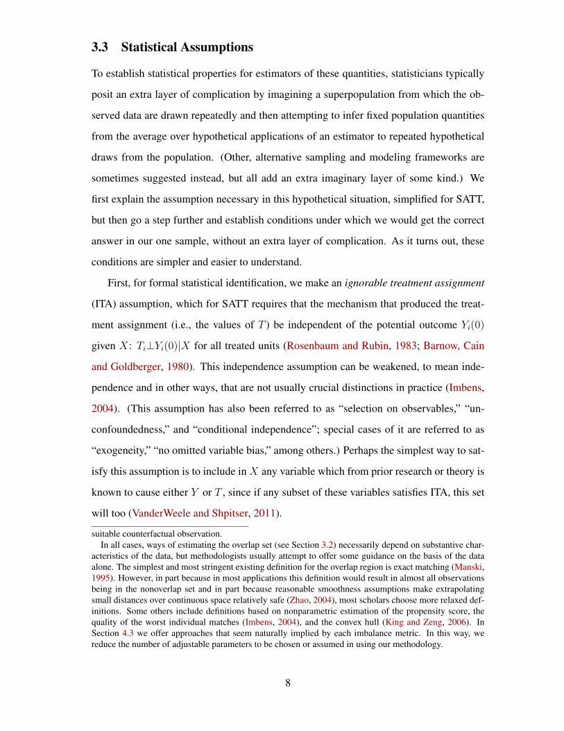
3.3 Statistical Assumptions
To establish statistical properties for estimators of these quantities, statisticians typically
posit an extra layer of complication by imagining a superpopulation from which the ob-
served data are drawn repeatedly and then attempting to infer fixed population quantities
from the average over hypothetical applications of an estimator to repeated hypothetical
draws from the population. (Other, alternative sampling and modeling frameworks are
sometimes suggested instead, but all add an extra imaginary layer of some kind.) We
first explain the assumption necessary in this hypothetical situation, simplified for SATT,
but then go a step further and establish conditions under which we would get the correct
answer in our one sample, without an extra layer of complication. As it turns out, these
conditions are simpler and easier to understand.
First, for formal statistical identification, we make an ignorable treatment assignment
(ITA) assumption, which for SATT requires that the mechanism that produced the treat-
ment assignment (i.e., the values of T ) be independent of the potential outcome Yi(0)
given X: Ti⊥Yi(0)|X for all treated units (Rosenbaum and Rubin, 1983; Barnow, Cain
and Goldberger, 1980). This independence assumption can be weakened, to mean inde-
pendence and in other ways, that are not usually crucial distinctions in practice (Imbens,
2004). (This assumption has also been referred to as “selection on observables,” “un-
confoundedness,” and “conditional independence”; special cases of it are referred to as
“exogeneity,” “no omitted variable bias,” among others.) Perhaps the simplest way to sat-
isfy this assumption is to include in X any variable which from prior research or theory is
known to cause either Y or T , since if any subset of these variables satisfies ITA, this set
will too (VanderWeele and Shpitser, 2011).
suitable counterfactual observation.In all cases, ways of estimating the overlap set (see Section 3.2) necessarily depend on substantive char-
acteristics of the data, but methodologists usually attempt to offer some guidance on the basis of the dataalone. The simplest and most stringent existing definition for the overlap region is exact matching (Manski,1995). However, in part because in most applications this definition would result in almost all observationsbeing in the nonoverlap set and in part because reasonable smoothness assumptions make extrapolatingsmall distances over continuous space relatively safe (Zhao, 2004), most scholars choose more relaxed def-initions. Some others include definitions based on nonparametric estimation of the propensity score, thequality of the worst individual matches (Imbens, 2004), and the convex hull (King and Zeng, 2006). InSection 4.3 we offer approaches that seem naturally implied by each imbalance metric. In this way, wereduce the number of adjustable parameters to be chosen or assumed in using our methodology.
8
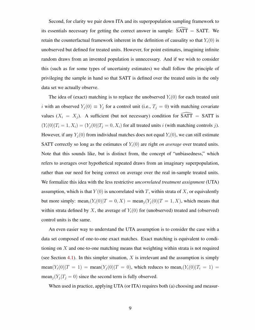
Second, for clarity we pair down ITA and its superpopulation sampling framework to
its essentials necessary for getting the correct answer in sample: SATT = SATT. We
retain the counterfactual framework inherent in the definition of causality so that Yi(0) is
unobserved but defined for treated units. However, for point estimates, imagining infinite
random draws from an invented population is unnecessary. And if we wish to consider
this (such as for some types of uncertainty estimates) we shall follow the principle of
privileging the sample in hand so that SATT is defined over the treated units in the only
data set we actually observe.
The idea of (exact) matching is to replace the unobserved Yi(0) for each treated unit
i with an observed Yj(0) ≡ Yj for a control unit (i.e., Tj = 0) with matching covariate
values (Xi = Xj). A sufficient (but not necessary) condition for SATT = SATT is
(Yi(0)|Ti = 1, Xi) = (Yj(0)|Tj = 0, Xi) for all treated units i (with matching controls j).
However, if any Yj(0) from individual matches does not equal Yi(0), we can still estimate
SATT correctly so long as the estimates of Yi(0) are right on average over treated units.
Note that this sounds like, but is distinct from, the concept of “unbiasedness,” which
refers to averages over hypothetical repeated draws from an imaginary superpopulation,
rather than our need for being correct on average over the real in-sample treated units.
We formalize this idea with the less restrictive uncorrelated treatment assignment (UTA)
assumption, which is that Y (0) is uncorrelated with T , within strata of X , or equivalently
but more simply: meani(Yi(0)|T = 0, X) = meanj(Yj(0)|T = 1, X), which means that
within strata defined by X , the average of Yi(0) for (unobserved) treated and (observed)
control units is the same.
An even easier way to understand the UTA assumption is to consider the case with a
data set composed of one-to-one exact matches. Exact matching is equivalent to condi-
tioning on X and one-to-one matching means that weighting within strata is not required
(see Section 4.1). In this simpler situation, X is irrelevant and the assumption is simply
mean(Yi(0)|T = 1) = mean(Yj(0)|T = 0), which reduces to meani(Yi(0)|Ti = 1) =
meanj(Yj|Tj = 0) since the second term is fully observed.
When used in practice, applying UTA (or ITA) requires both (a) choosing and measur-
9

ing the correct variables in X and (b) using an analysis method that controls sufficiently
for the measured X so that T and Y (0) are sufficiently close to unrelated that any biases
that a relationship generates can for practical purposes be ignored (i.e., such as if they are
much smaller than the size of the quantities being estimated). Virtually all observational
data analysis approaches, including matching and modeling methods, assume (a) holds as
a result of choices by the investigator. This includes defining which variables are included
in X and ensuring that the definition of each of the variables has a meaningful scaling
or metric. Then, given the choice of X , the methods distinguish themselves by how they
implement approximations to (b) given the choice for the definition of X .
4 Matching Frontier ComponentsThe matching frontier (defined formally in Section 5) requires the choice of options for
four separate components. In addition to the quantity of interest (Section 3.2), they include
and we now describe fixed- v. variable-ratio matching (Section 4.1), a definition for the
units to be dropped (Section 4.2), and the imbalance metric (Section 4.3).
4.1 Fixed- or Variable-Ratio Matching
Some matching methods allow the ratio of treated to control units to vary, whereas others
restrict them to have a fixed ratio throughout a matched data set. Fixed-ratio matching
can be less efficient than variable ratio matching because some pruning usually occurs
solely to meet this restriction. However, an important goal of matching is simplicity
and encouraging researchers to understand and use this powerful procedure, and so the
ability to match without having to modify existing analysis procedures, remains popular.
(Fixed-ratio matching is also useful in large data sets where the primary goal is reducing
bias.) Indeed, most applications involve the even more restrictive requirement of 1-to-1
matching, or sometimes 1-to-p matching with larger p.
In fixed-ratio matching, SATT can be estimated by a simple difference in means be-
tween the treated and control groups: meani∈{T=1}(Yi)−meanj∈{T=0}(Yj).
In variable-ratio matching, we can estimate the TE within each matched stratum s by
a simple difference in means: meani∈s,{T=1}(Yi) − meanj∈s,{T=0}(Yj). However, aggre-
gating up to SATT requires weighting, with the stratum-level TE weighted according to
10

the number of treated units. Equivalently, a weighted difference in means can be com-
puted, with weights W such that each treated unit i receives a weight of Wi = 1, and each
control unit j receives a weight of Wj = (m0/m1)[(ms1)/(ms0)] where m0 and m1 are
respectively the number of control and treated units in the data set, and ms1 and ms0 are
the number of treated and control units in the stratum containing observation j.3
4.2 Defining the Number of Units
The size and construction of a matched data set influences the variance of the causal
effect estimated from it. Under SATT, the number of treated units remain fixed and so we
measure the data set size by the number of control units. For FSATT, we measure the total
number of observations .
For both quantities of interest, we will ultimately use an estimator equal to or a func-
tion of the difference in means of Y between the treated and control groups. The variance
of this estimator is proportional to 1nT
+ 1nC
, where nT and nC are the number of treated
and control units in the matched set. Thus, the variance of the estimator is largely driven
by min(nT , nC), and so we will also consult this as an indicator of the size of the data set.
To simplify notation in these different situations, we choose a method of counting
from those above and let N denote the number of these units in the original data and n the
number in a matched set, with n ≤ N . In our graphs, we will represent this information
as the number of units pruned, which is scaled in the same direction as the variance.
4.3 Imbalance Metrics
An imbalance measure is a (nondegenerate) indicator of the difference between the mul-
tivariate empirical densities of the k-dimensional covariate vectors of treated X1 and con-
trol X0 units for any data set (i.e., before or after matching). Our concept of a matching
frontier, which we define more precisely below, applies to any imbalance measure a re-
searcher may choose. We ease this choice by narrowing down the reasonable possibilities
from measures to metrics and then discuss five examples of continuous and discrete fami-
lies of these metrics. For each example, we give metrics most appropriate for FSATT and
SATT when feasible.3See j.mp/CEMweights for further explanation of these weights. Also, for simplicity, we define any
reuse of control units to match more than one control as variable-ratio matching.
11

Measures v. Metrics To narrow down the possible measures to study, we restrict our-
selves to the more specific concept of an imbalance metric, which is a function d :
[(m0 × k) × (m1 × k)] → [0,∞] with three properties, required for a generic semi-
distance:
1. Nonnegativeness: d(X0, X1) ≥ 0.
2. Symmetry: d(X0, X1) = d(X1, X0) (i.e., replacing T with 1 − T will have noeffect).
3. Triangle inequality: d(X0, X1) + d(X1, Z) ≥ d(X0, Z), given any k-vector Z.
Imbalance measures that are not metrics have been proposed and are used sometimes,
but they add complications such as logical inconsistencies without conferring obvious
benefits. Fortunately, numerous imbalance metrics have been proposed or could be con-
structed.
Continuous Imbalance Metrics The core building block of a continuous imbalance
metric is a (semi-)distance D(Xi, Xj) between two k-dimensional vectors Xi and Xj , cor-
responding to observations i and j. For example, the Mahalanobis distance is D(Xi, Xj) =√(Xi −Xj)S−1(Xi −Xj), where S is the sample covariance matrix of the original data
X . The Euclidean distance would result from redefining S as the identity matrix. Numer-
ous other existing definitions of continuous metrics could be used instead. Although one
can always define a data set that will produce large differences between any two metrics,
in practice the differences among the choice of these metrics are usually not large or at
least not the most influential choice in most data analysis problems (Zhao, 2004; Imbens,
2004). We use the most common choice of the Mahalanobis distance below for illus-
tration, but any of the others could be substituted. In real applications, scholars should
choose variables, the coding for the variables, and the imbalance metric together to reflect
their substantive concerns: with this method as with most others, the more substantive
knowledge one encodes in the procedure, the better the result will be.
To get from a distance between two individual observations to an imbalance metric
comparing two sets of observations, we need to aggregate the distance calculations over
observations in one of two ways. One way to do this is with the Average Mahalanobis
12

Imbalance (AMI) metric, which is the distance between each unit i and the closest unit in
the opposite group, averaged over all units: D = meani[D(Xi, Xj(i))], where the closest
unit in the opposite group is Xj(i) = argmin Xj |j∈{1−Ti}[D(Xi, Xj)] and {1 − Ti} is the
set of units in the (treatment or control) group that does not contain i.
For SATT, it is helpful to have a way to identify the overlap and nonoverlap sets. A
natural way to do this for continuous metrics is to define the nonoverlap region as the set of
treated units for which no control unit has chosen it as a match. More precisely, denote the
(closest) treated unit i that control unit j matches to by j(i) ≡ argmin i|i∈{T=1}[D(Xi, Xj)].
Then define the overlap and nonoverlap sets, respectively, as
O ≡ {j(i) | j ∈ {T = 0}} (2)
NO ≡ {i | i ∈ {T = 1} ∧ {i 6∈ O}} (3)
where ∧ means “and,” connecting two statements required to hold.
Discrete Imbalance Metrics Discrete imbalance metrics indicate the difference be-
tween the multivariate histograms of the treated and control groups, defined by fixed bin
sizes H . Let f`1···`k be the relative empirical frequency of treated units in a bin with coor-
dinates on each of the X variables as `1 · · · `k so that f`1···`k = nT`1···`k/nT where nT`1···`k
is the number of treated units in stratum `1 · · · `k and nT is the number of treated units in
all strata. We define g`1···`k similarly among control units. Then, among the many possible
metrics built from these components, we consider two:
L1(H) =1
2
∑(`1···`k)∈H
|f`1···`k − g`1···`k | (4)
and
L2(H) =1
2
√ ∑(`1···`k)∈H
(f`1···`k − g`1···`k)2 (5)
To remove the dependence on H , Iacus, King and Porro (2011a) define L1 as the median
value of L1(H) from all possible bin sizes H in the original unmatched data (approxi-
mated by random simulation); we use the same value of H to define L2. The typically
numerous empty cells of each of the multivariate histograms do not affect L1 and L2, and
so the summation in (4) and (5) each have at most only n nonzero terms.
13

When used for creating SATT frontiers, these discrete metrics suggest a natural indi-
cator of the nonoverlap region: all observations in bins with either one or more treated
units and no controls or one or more control units and no treateds.
With variable-ratio matching, and the corresponding weights allowed in the calcula-
tion of L1, the metric is by definition 0 in the overlap region. With fixed-ratio matching,
L1 will improve as the heights of the treated and control histogram bars within each bin in
the overlap region equalize. (In other words, what the weights, included for variable-ratio
matching, do is to equalize the heights of the histograms without pruning observations.)
Adjusting Imbalance Metrics for Relative Importance Every imbalance metric is
conditional on a definition of the variables in X , and so researchers must think carefully
about what variables may be sufficient in their application. This choice also involves care-
fully defining the measurement or scaling of each covariate so that it makes sense (e.g.,
ensuring interval-level measurement for continuous distance metrics) and reflects prior
information about its importance in terms of its relationship with Y |T . In almost all areas
of applied research, the most important covariates are well known to researchers — such
as age, sex, and education in public health, or partisan identification and ideology in polit-
ical science. Since bias is a function of both importance and imbalance, and matching can
only affect the latter (Imai, King and Stuart, 2008), we will want to require better matches
on important covariates. This is easy to do in the context of most imbalance metrics by
adjusting weights used in continuous metrics (such as S in average Mahalanobis or Eu-
clidean distance; see Greevy et al. 2012) or variable-specific coarsening used in discrete
metrics (such as H in L1).
5 Constructing FrontiersNow that we have given our notation and components of a frontier, we offer a formal
definition along with algorithms for calculating the (theoretical) frontier directly.
5.1 Definition
Begin by choosing an imbalance metric d(x0, x1) (see Section 4.3), a quantity of interest
Q (SATT or FSATT described in Section 3.2), whether to use weights (to allow variable-
ratio matching) or no weights (as in fixed-ratio matching) R (Section 4.1), and a definition
14

for the number of units U (Section 4.2). We will consider all matched data set sizes from
the original N , all the way down n = N,N − 1, N − 2 . . . , 2.
For quantity of interest SATT, where only control units are pruned, denoteXn as the set
of all(Nn
)possible data sets formed by taking every combination of n rows (observations)
from the (N × k) control group matrix X0. Then denote the combined set of all sets Xn
as X ≡ {Xn | n ∈ {N,N − 1, . . . , 1}}. This combined set X is (by adding the null set)
the power set of rows of X0, containing (a gargantuan) 2N elements. For example, if the
original data set contains merely N = 300 observations, the number of elements of this
set exceeds current estimates of the number of elementary particles in the universe. The
task of finding the frontier requires identifying a particular optimum over the entire power
set. As it turns out, with our new algorithms, this task, as we show below, can often be
accomplished fast and efficiently.
To be more specific, first identify an element (i.e., data set) of Xn with the lowest
imbalance for a given matched sample size n, and the choices of Q, U , and R:
xn = argminx0∈Xn
d(x0, x1), given Q,R, and U. (6)
where for convenience when necessary we define the argmin function in the case of
nonunique minima as a random draw from the set of data sets with the same minimum
imbalance. We then create a set of all these minima {xN , xN−1, . . . , 1}, and finally define
the matching frontier as the subset F of these minima after imposing monotonicity, which
involves eliminating any element which has higher imbalance with fewer observations:
F ≡ {xn | (n ∈ {N,N − 1, . . . , 1}) ∧ (dn−1 ≤ dn)} (7)
where dn = d(xn, x1). We represent a frontier by plotting the number of observations
pruned N − n horizontally and dn vertically.
For simplicity, we will focus on SATT here, but our description also generalizes to
FSATT by defining Xn as the set of all combinations of the entire data matrix (X ′0, X′1)′
taken n at a time.
15

5.2 Algorithms
Calculating the frontier requires finding a data subset of size n with the lowest imbalance
possible chosen from the original data of size N for each possible n (N > n) — given
choices of the quantity of interest (and thus the definition of the units to be pruned),
fixed- or variable-ratio matching, and an imbalance metric, along with the monotonicity
restriction.
Adapting existing approaches to algorithms for this task is impractical. The most
straightforward would involve directly evaluating the imbalance of the power set of all
possible subsets of observations. For even moderate data set sizes, this would take con-
siderably longer than the expected lives of most researchers (and for reasonably sized data
sets far longer than life has been on the planet). Another approach could involve evaluat-
ing only a sample of all possible subsets, but this would be biased, usually not reaching
the optimum (for the same reason that estimating a maximum by sampling is an under-
estimate). Finally, adapting general purpose numerical optimization procedures designed
for similar but different purposes, such as Diamond and Sekhon (2012), would take many
years and in any event are not guaranteed to reach the optimum.
The contribution of our algorithms, then, is not that they can find the optimum, but
that they can find it fast. Our solution is to offer analytical rather than numerical solutions
to this optimization problem cases by leveraging the properties of specific imbalance met-
rics. The key to each is developing greedy algorithms that return optimal results.
We now outline algorithms we developed for calculating each of four families of
matching frontiers, with many possible members of each. We leave to future research
the derivation of algorithms for other families of matching frontiers (defined by choosing
among permutations of the choices defined in Section 5.1, and finding a feasible algo-
rithm). In all cases with SATT frontiers, we first remove the nonoverlap set and then
compute the remaining frontier within the overlap set. FSATT frontiers do not require
this separate step.
16

5.2.1 Continuous, FSATT, Variable Ratio
Our first family of algorithms is based on the average continuous imbalance metric for
FSATT with variable ratio matching. We illustrate this with the AMI metric, although
any other continuous metric could be substituted. Define N as the number of units in
the original data, n as the number that have not yet been pruned, and Dn as the current
matched data set. Then our algorithm requires five steps:
1. Begin with N = n.
2. Match each observation i (i = 1, . . . , N ) to the nearest observation j(i) in the
opposite treatment condition {1 − Ti}; this matched observation has index j(i) =
argmin j∈{1−Ti}[D(Xi, Xj)], and distance dj(i) ≡ D(Xi, Xj(i)).
3. Calculate AMI for Dn.
4. Prune from Dn the unit or units with distance dj(i) equal to max(dj(i)|i ∈ Dn).
Redefine n as the number of units remaining in newly pruned data set Dn.
5. If n > 2 and AMI > 0, go to Step 3; else stop.
This is a greedy algorithm, but we now prove that it is optimal by proving two claims
that, if true, are sufficient to establish optimality. Below, we offer a simple example.
Claim 1. For each unit i remaining in the data set, the nearest unit (or units) in the
opposite treatment regime j(i) (defined in Step 2) remains unchanged as units are pruned
in Step 4.
Claim 2. The subset Dn with the smallest AMI, among all(Nn
)subsets of DN , is that
defined in Step 4 of the algorithm.
Given Claim 1, Claim 2 is true by definition since Dn includes the n smallest distances
within DN .
We prove Claim 1 by contradiction. First assume that the next unit to be prunned is
the nearest match for a unit not yet pruned (hence requiring the data set to be rematched).
However, this is impossible because the unit not yet pruned would have had to have a
17
6 8 10 12 14 16 18
4
6
8
10
12
14
Covariate #1
Cov
aria
te #
2 7
3
6
8
3
1
5 8
2●
●
●
●
●
●
●
Number of Observations Pruned
Mea
n M
ahal
anob
is D
ista
nce
0 1 2 3 4 5 6 7 8
1.75
2.00
2.25
2.50
2.75
3.00
3.25
3.50
3.75
4.00
4.25
4.50
3
67
8
1
2
3
5
8
,
,
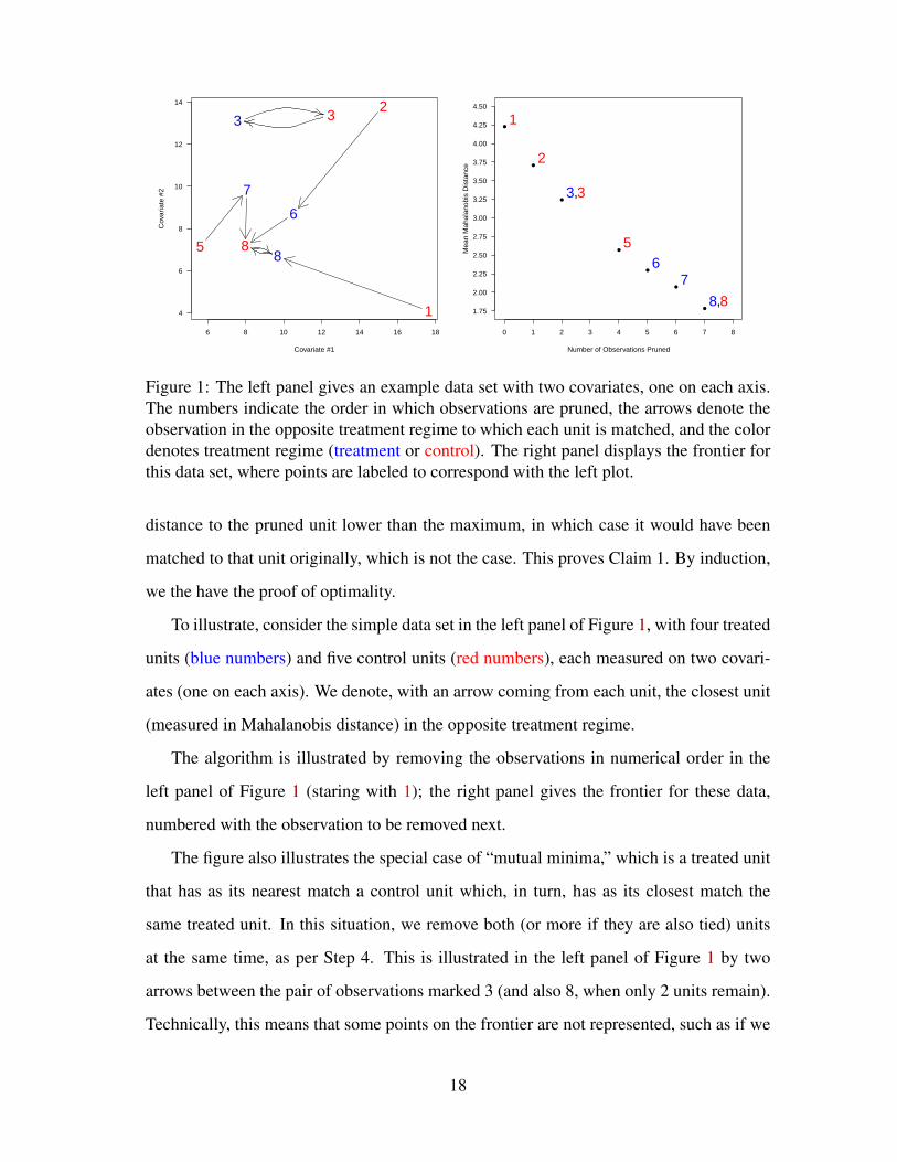
Figure 1: The left panel gives an example data set with two covariates, one on each axis.The numbers indicate the order in which observations are pruned, the arrows denote theobservation in the opposite treatment regime to which each unit is matched, and the colordenotes treatment regime (treatment or control). The right panel displays the frontier forthis data set, where points are labeled to correspond with the left plot.
distance to the pruned unit lower than the maximum, in which case it would have been
matched to that unit originally, which is not the case. This proves Claim 1. By induction,
we the have the proof of optimality.
To illustrate, consider the simple data set in the left panel of Figure 1, with four treated
units (blue numbers) and five control units (red numbers), each measured on two covari-
ates (one on each axis). We denote, with an arrow coming from each unit, the closest unit
(measured in Mahalanobis distance) in the opposite treatment regime.
The algorithm is illustrated by removing the observations in numerical order in the
left panel of Figure 1 (staring with 1); the right panel gives the frontier for these data,
numbered with the observation to be removed next.
The figure also illustrates the special case of “mutual minima,” which is a treated unit
that has as its nearest match a control unit which, in turn, has as its closest match the
same treated unit. In this situation, we remove both (or more if they are also tied) units
at the same time, as per Step 4. This is illustrated in the left panel of Figure 1 by two
arrows between the pair of observations marked 3 (and also 8, when only 2 units remain).
Technically, this means that some points on the frontier are not represented, such as if we
18

wished to prune exactly 3 observations in this simple example. Although we could fill
in these missing points by enumerating and checking all possible data sets this size, we
find that omitting them, and thus saving substantial computational time, is almost costless
from a practical point of view: a researcher who wants a data set of a particular sample
size would almost always be satisfied with a very slightly different sample size. With a
realistic sized data set, the missing points on the frontier, like discrete points in a (near)
continuous space, are graphically invisible and for all practical purposes substantively
irrelevant.4
Put differently, the intuition as to why the greedy algorithm is also optimal is that at
every point along the frontier, the closest match for each observation in the remaining
set is the same as that in the full set, which implies that (1) each observation contributes
a fixed distance to the average distance for the entire portion of the frontier in which it
remains in the sample and (2) observations do not need to be re-matched as others are
pruned.
5.2.2 Continuous, SATT, Variable Ratio
The SATT frontier is identical to the FSATT frontier when the SATT requirement of
keeping all treated units is not binding. This occurs when the maxi dj(i) calculation in
the FSATT algorithm leads us to prune only control units. Usually, this is the case for
some portion of the frontier, but not the whole frontier. When the calculable part of this
SATT frontier is not sufficient, part of each matched data set along the rest of the frontier
will have a nonoverlap region, requiring extrapolation. In these situations, we recom-
mend using the FSATT algorithm for the overlap region, extrapolating to the remaining
nonoverlap region and combining the results as per Equation 1.
5.2.3 Discrete, FSATT, Variable Ratio
As a third family of frontiers, we can easily construct a discrete algorithm for FSATT
with variable ratio matching, using L1 for exposition. With variable ratio matching in
4It is important to note that the missing points on the frontier cannot violate the monotonicity constraint.If the point after the gap contains n observations, those n observations are the n observations with theclosest matches. Therefore, there can be no set of n + 1 observations (say in the gap) with a lower meandistance than that in the n observations contained at the defined point, because the additional observationmust have a distance equal to or greater than the greatest distance in the existing n observations.
19

discrete metrics, weighting eliminates all imbalance in the overlap set, making this frontier
a simple step function with only two steps. The first step is defined by L1 for the original
data and the second is L1 after the nonoverlap region has been removed. Within each
step, we could remove observations randomly one at a time, but since imbalance does not
decline as a result it makes more sense to only define the frontier for only these two points
on the horizontal axis.
If the binning H is chosen to be the same as the coarsening in coarsened exact match-
ing (CEM), the second step corresponds exactly to the observations retained by CEM
(Iacus, King and Porro, 2011a,b).
5.2.4 Discrete, SATT, Fixed-Ratio
A final family of frontiers is for discrete metrics, such as L1 or L2, for quantity of interest
SATT with fixed-ratio matching. To define the algorithm, first let biT and biC be the
numbers, and piT = biT/nT and piC = biC/nC be the proportions, of treated and control
units in bin i (i ∈ {1, . . . , B}) in the L1 multivariate histogram, where nT =∑B
i=1 biT
and nC =∑B
i=1 biC are the total numbers of treated and control units.
To prune k observations optimally (that is with minimum L1 imbalance) from a data
set of sized N , we offer this algorithm:
1. Define p′iC = biC/(nC − k).
2. Prune up to k units from any bin i where after pruning p′iC ≥ piT holds.
3. If k units have not been pruned in step 2, prune the remaining k′ units from the bins
with the k′ largest differences piC − p′iT .
An optimal frontier can then be formed by applying this algorithm with k = 1 prunned
and increasing until small numbers of observations results in nonmonotonicities in L1.
The discreteness of the L1 imbalance metric means that multiple data sets have equiva-
lent values of the imbalance metric for each number of units pruned. Indeed, it is possible
with this general algorithm to generate one data set with k− 1 pruned and another with k
pruned that differ with respect to many more than one unit. In fact, even more complicated
is that units can be added, removed, and added back for different adjacent points on the
20

frontier. This of course does not invalidate the algorithm, but it would make the resulting
frontier difficult and use in applied research. Thus, to make this approach easier to use,
we choose a greedy algorithm which is a special case of this general optimal algorithm.
The greedy algorithm is faster but more importantly it, by definition, never needs to put a
unit back in a data set once it had been pruned.
Our greedy (and also optimal) algorithm is as follows. Starting with the full data set
N = n,
1. Compute and record the value of L1 and the number of units n.
2. Prune a control unit from the bin with the maximum difference between the pro-
portions of treated and control units, such that there are more controls than treateds.
That is, prune a unit from bin f(i), where
f(i) = argmaxi∈{nC>nT }
|pic − pit| (8)
3. If L1 is larger than the previous iteration, stop; otherwise go to step 1.
To understand this algorithm intuitively, first note that deleting a control unit from
any bin with more controls than treateds changes L1 by an equal amount (because we are
summing over bins normalized by the total number of controls, rather than by the number
of controls in any particular bin). When we delete a control unit one bin, the relative size
of all the other bins increase slightly, because all the bins must always sum to 1. Deleting
controls from bins with the greatest relative difference, as we do, prevents the relative
number of treated units from ever overtaking the relative number of controls in any bin,
and guarantees that this greedy algorithm is optimal.
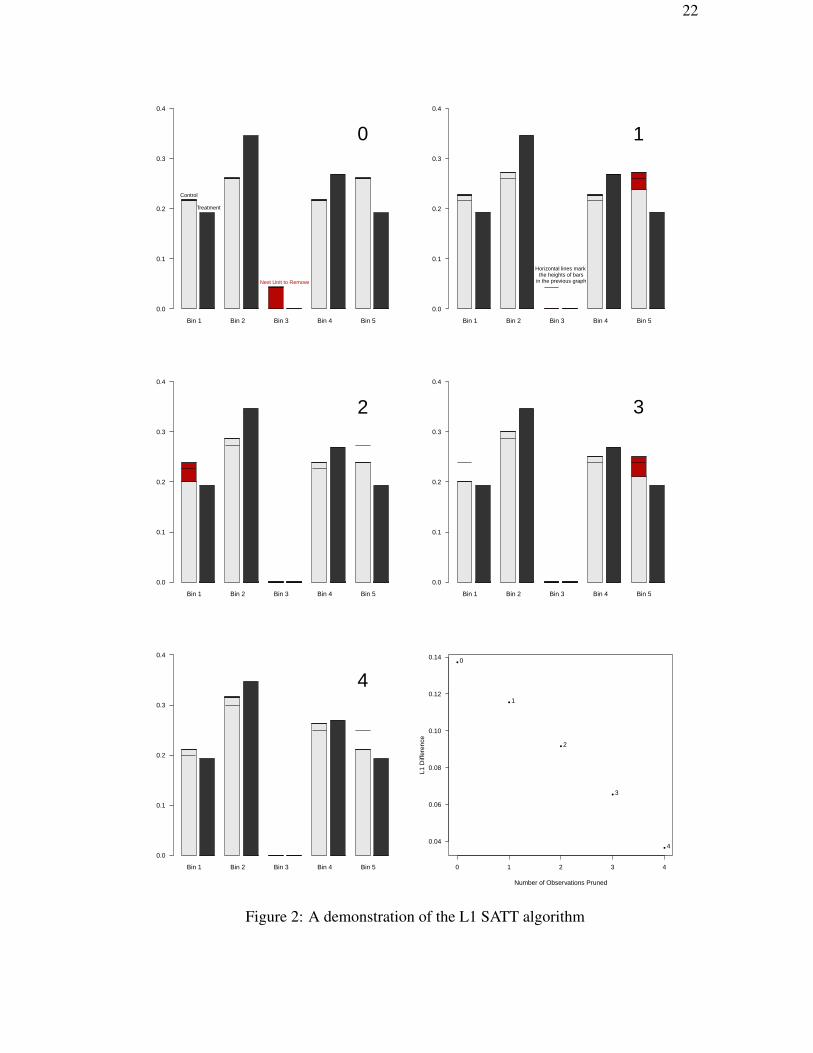
To illustrate the greedy version of this optimal algorithm, Figure 2 gives a simple
univariate example. Panel 0 in the top left represents the original data set with a histogram
in gray for controls and black for treateds. The L1 imbalance metric for Panel 0 is reported
in the frontier (Figure 2, bottom right) marked as “0”. The red unit in Panel 0 is the next
control unit to be removed, in this case because it is in a bin without any treated units.
Then, Panel 1 (i.e., where 1 observation has been pruned) removes the red unit from
Panel 0, and renormalizes the height of all the bars with at least some control units so
21
22
Bin 1 Bin 2 Bin 3 Bin 4 Bin 5
0.0
0.1
0.2
0.3
0.4
Next Unit to Remove
Control
Treatment
0
Bin 1 Bin 2 Bin 3 Bin 4 Bin 5
0.0
0.1
0.2
0.3
0.4
Horizontal lines mark the heights of bars
in the previous graph
1
Bin 1 Bin 2 Bin 3 Bin 4 Bin 5
0.0
0.1
0.2
0.3
0.4
2
Bin 1 Bin 2 Bin 3 Bin 4 Bin 5
0.0
0.1
0.2
0.3
0.4
3
Bin 1 Bin 2 Bin 3 Bin 4 Bin 5
0.0
0.1
0.2
0.3
0.4
4●
●
●
●
●
0.04
0.06
0.08
0.10
0.12
0.14
Number of Observations Pruned
L1 D
iffer
ence
0
1
2
3
4
0 1 2 3 4
Figure 2: A demonstration of the L1 SATT algorithm

that they still sum to one. As indicated by the extra horizontal lines, reflecting the heights
of control histogram bars from the previous panel, the height of each of the remaining
the gray control histogram bars have increased slightly. The “1” point in the bottom
right panel in Figure 2 plots this point on the frontier. The red piece of Bin 5 in Panel 1
refers to the next observation to be removed, in this case because this bin has the largest
difference between control and treateds, among those with more controls than treateds
(i.e., Equation 8). Panels 2-4 repeat the same process as in Panel 1, until we get to Panel
4 where no additional progress can be made and the frontier is complete.
6 ApplicationsWe now apply our approach in two important applications. The first uses a SATT fron-
tier, so a direct comparison can be made between experiment and observational data sets.
The second uses a FSATT frontier in a purely observational study, and thus we focus on
understanding the new causal quantity being estimated.
6.1 Job Training
We begin with a data set compiled from the National Supported Work Demonstration
(NSWD) and the Current Population Survey (Lalonde, 1986; Dehejia and Wahba, 2002).
The first was an experimental intervention, while the second is a large observational data
collection appended to the 185 experimental treated units and used in the methodological
literature as a mock control group to test a method’s ability to recover the experimental
effect from observational data. Although our purpose is only to illustrate the use of the
matching frontier, we use the data in the same way.
As is standard in the use of these data, we match on age, education, race (black or
Hispanic), marital status, whether or not the subject has a college degree, earnings in
1974, earnings in 1975, and indicators for whether or not the subject was unemployed in
1974 and 1975. Earnings in 1978 is the outcome variable. To ensure a direct comparison,
we estimate the SATT fixed ratio frontier, and thus prune only control units. We give the
full matching frontier in the top-left panel of Figure 3, and, in the two lower panels, the
effect estimates for every point on the frontier (the lower-left panel displays estimates over
the full frontier and the lower-right panel zooms in on the final portion of the frontier).
23
0 5000 10000 15000
0.5
0.6
0.7
0.8
0.9
1.0
Number of Observations Pruned
L1
0 5000 10000 15000
−10
000
−60
00−
2000
020
00
Number of Observations Pruned
Est
imat
e
15500 15700 15900 16100
−10
000
−60
00−
2000
020
00
Number of Observations Pruned
Est
imat
e
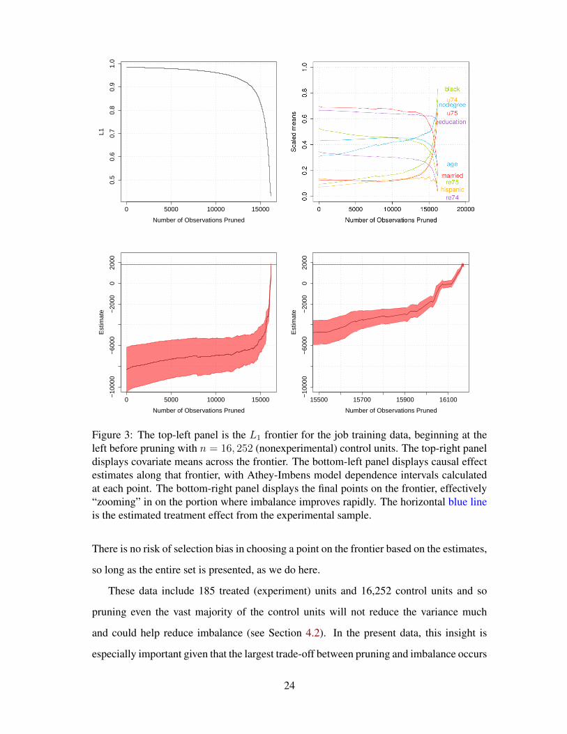
Figure 3: The top-left panel is the L1 frontier for the job training data, beginning at theleft before pruning with n = 16, 252 (nonexperimental) control units. The top-right paneldisplays covariate means across the frontier. The bottom-left panel displays causal effectestimates along that frontier, with Athey-Imbens model dependence intervals calculatedat each point. The bottom-right panel displays the final points on the frontier, effectively“zooming” in on the portion where imbalance improves rapidly. The horizontal blue lineis the estimated treatment effect from the experimental sample.
There is no risk of selection bias in choosing a point on the frontier based on the estimates,
so long as the entire set is presented, as we do here.
These data include 185 treated (experiment) units and 16,252 control units and so
pruning even the vast majority of the control units will not reduce the variance much
and could help reduce imbalance (see Section 4.2). In the present data, this insight is
especially important given that the largest trade-off between pruning and imbalance occurs
24

after most of the observations are pruned; this can be seen at the right of the left panel of
Figure 3, where the frontier drops precipitously.
The right panel gives the causal effect estimates, where the apparent advantages of
pruning most of the cases can be seen. Over most of the range of the frontier, causal
estimates from the (badly matched) data do not move much from the original unmatched
estimate, −$8,334, which would indicateconfi that this job training program was a disas-
ter. Then after the fast drop in imbalance (after pruning about 15,000 mostly irrelevant
observations), the estimates rise fast, and ultimately intersect with the experimental esti-
mate of the training program producing a benefit of $1,794 per trainee (denoted by the
red horizontal line). Overall, the frontier reveals the whole range of possible conclusions
as a function of the full bias-variance trade off. The right panel also gives Athey-Imbens
model dependence intervals (Athey and Imbens, 2015) around the point estimates5; the
width of these are controlled by the model dependence remaining in the data and so de-
crease as balance improves across the frontier. Correspondingly, the largest change in
model dependence occurs near the end of the frontier, where imbalance improves the
most.
6.2 Sex and Judging
For our second example, we replicate Boyd, Epstein and Martin (2010), who offer a rig-
orous analysis of the effect of sex on judicial decision making. They first review the
large number of theoretical and empirical articles addressed to this question and write that
“roughly one-third purport to demonstrate clear panel or individual effects, a third report
mixed results, and the final third find no sex-based differences whatsoever.” These prior
articles all use similar parametric regression models (usually logit or probit) and related
data sets. To tame this remarkable level of model dependence, they introduce nearest
neighbor propensity score matching to this literature, and find no effects of sex on judg-
ing in every one of 13 policy areas except for sex discrimination, which makes good sense
substantively. The authors also offer a spirited argument for bringing “promising devel-
5Athey and Imbens (2015) propose “a scalar measure of the sensitivity of the estimates to a range ofalternative models.” To compute this measure, investigators estimate the quantity of interest with a basemodel, after which the quantity of interest is estimated in subsamples divided according to covariate values.The deviation of these subsample estimates from the base estimate is then a measure of model dependence.
25

opments in the statistical sciences” to important substantive questions in judicial politics,
and so we follow their lead here too. We thus follow their inclinations but with meth-
ods developed after the publication of their article, by seeing whether our more powerful
approach can detect results not previously possible.
Boyd, Epstein and Martin (2010) motivate their study by clarifying four different
mechanisms by which sex might influence judicial outcomes, each with distinct empir-
ical implications. First, different voice, in which “males and females develop distinct
worldviews and see themselves as differentially connected to society.” This account sug-
gests that males and females should rule differently across a broad range of issues, even
those with no clear connection to sex. Second, representational, which posits that “female
judges serve as representatives of their class and so work toward its protection in litigation
of direct interest.” This theory predicts that males and females judge differently on issues
of immediate concern to women. Third, informational, which argues that “women pos-
sess unique and valuable information emanating from shared professional experiences.”
Here, women judge differently on the basis of their unique information and experience,
and so might differ from men on issues over which they have distinct experiences, even
if not related to sex. Finally, organizational, in which “Male and female judges undergo
identical professional training, obtain their jobs through the same procedures, and con-
front similar constraints once on the bench.” This theory predicts than men and women
do not judge differentially.
Boyd, Epstein and Martin (2010) argue that their results — that male and females
judge differently only in sex discrimination cases — are “consistent with an information
account of gendered judging.” Of course, their results are also consistent with repre-
sentational theories. Indeed, as Boyd, Epstein and Martin (2010) argue, women might
judge differently on sex discrimination because they have different information as a re-
sult of shared experiences with discrimination. But it is also possible that women judge
differently on sex discrimination as a way to protect other women, consistent with repre-
sentational accounts.
One way to use our new methodological approach is to attempt to distinguish between
26

these conflicting interpretations of the effects of sex. To do so, we analyze cases on an
issue in which we expect to observe a difference if and only if the informational account is
true. That is, an issue area where the unique experiences of women might lead to informa-
tional differences between men and women but that nonetheless does not directly concern
the interests of women. For this analysis, we consider cases related to discrimination on
the basis of race. Because women have shared experiences with discrimination, they have
informational differences from men relevant to this issue area. However, judgements on
racial discrimination do not have direct consequences for women more broadly. This issue
area is the only such issue area that allows us to distinguish between these two accounts
and for which we also have a suitable amount of available data.
Thus, using their data, we reanalyze race discrimination cases made on the basis of
Title VII. In their original analysis, Boyd, Epstein and Martin (2010) found a null effect
with this issue area, both before and after matching. We now show, with our method
which enables us to analyze data with less dependence and bias than previous matching
approaches, that female judges rule differently on race discrimination cases. We show
that differences in male and female judgements are at least in part due to informational
differences.
We arranged the data from Boyd, Epstein and Martin (2010) so that the unit of analysis
is the appellate court case, the level at which decisions are made. For example, the fourth
observation in our data set is Swinton v. Potomac Corporation, which was decided in 2001
by the Ninth Circuit Court of Appeals and at the time was composed of Judges William A.
Fletcher, Johnnie B. Rawlinson, and Margaret M. McKeown. Our treatment is whether or
not at least one female judge was included in the three-judge panel. In Swinton v. Potomac
Corporation, Judges Rawlinson and McKeown are female and so this observation is in
the treatment group. For each appellate court case, we use the following covariates: (1)
median ideology as measured by Judicial Common Space scores (Epstein et al., 2007;
Giles, Hettinger and Peppers, 2001), (2) median age, (3) an indicator for at least one
racial minority among the three judges, (4) an indicator for ideological direction of the
lower court’s decision, (5) an indicator for whether a majority of the judges on the three-
27

judge panel were nominated by Republicans, and (6) an indicator for whether a majority
of the judges on the panel had judicial experience prior to their nomination. In Swinton v.
Potomac Corporation, for example, the median ideology was at the 20th percentile in the
distribution of judges who ruled on a Title VII-race discrimination case and in the 10th
percentile in the distribution of median ideologies, where lower scores are more liberal
and higher scores are more conservative. This is unsurprising, as all three judges were
nominated by President Clinton in either 1998 or 2000. Our outcome is the ideological
direction of the decision — either liberal or conservative — and unsurprisingly, the ruling
on Swinton v. Potomac Corporation was a liberal one. For our analysis, we use these six
covariates to construct a Mahalanobis frontier for the estimation of FSATT.
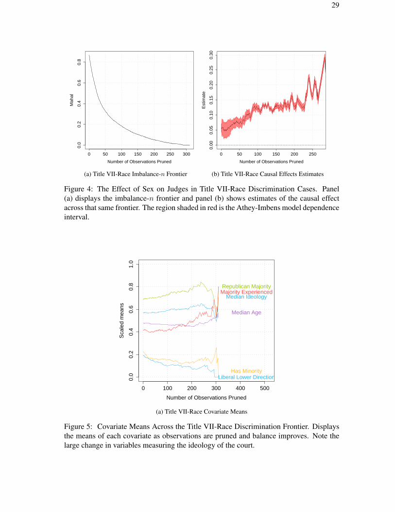
We present the matching frontier in Figure 4, panel (a); in contrast to our previous
example, most of the reduction in imbalance for observations pruned happens early on,
but substantial imbalance reduction continues through the entire range. Our substantive
results can be found in panel (b), which indicates that having a female judge increases the
probability of a liberal decision, over the entire range. The vertical axis quantifies the sub-
stantial effect we see in terms of the reduction in probability, from about 0.05 with few
observations pruned and higher levels of model dependence to 0.25 with many pruned
and lower levels. Most importantly in this case, the point estimate of the causal effect
increases as balance improves and we zero in on a data subset more closely approximat-
ing a randomized experiment. Correspondingly, model dependence, measured with red
intervals around each line, decreases.
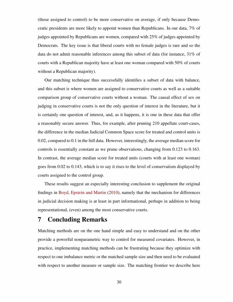
Because we pruned both treated and control units in this example, we must carefully
consider how the quantity of interest changes as balance improves. Interestingly, the best
balance exists within more conservative courts (and thus the effect we find in Figure 4
is among these courts). To see this, note that in Figure 5, which plots the means of each
covariate as observations are pruned, variables associated with the court ideology changed
the most, and all moved in a conservative direction.
More specifically, Republican majority has the largest difference in means, followed
by median ideology and median age. That makes sense, as we expect all-male panels
28
29
0 50 100 150 200 250 300
0.0
0.2
0.4
0.6
0.8
Number of Observations Pruned
Mah
al
(a) Title VII-Race Imbalance-n Frontier
0 50 100 150 200 250
0.00
0.05
0.10
0.15
0.20
0.25
0.30
Number of Observations Pruned
Est
imat
e
(b) Title VII-Race Causal Effects Estimates
Figure 4: The Effect of Sex on Judges in Title VII-Race Discrimination Cases. Panel(a) displays the imbalance-n frontier and panel (b) shows estimates of the causal effectacross that same frontier. The region shaded in red is the Athey-Imbens model dependenceinterval.
0 100 200 300 400 500
0.0
0.2
0.4
0.6
0.8
1.0
Number of Observations Pruned
Sca
led
mea
ns
Median Ideology
Median Age
Republican Majority
Has Minority
Majority Experienced
Liberal Lower Direction
(a) Title VII-Race Covariate Means
Figure 5: Covariate Means Across the Title VII-Race Discrimination Frontier. Displaysthe means of each covariate as observations are pruned and balance improves. Note thelarge change in variables measuring the ideology of the court.
(those assigned to control) to be more conservative on average, if only because Demo-
cratic presidents are more likely to appoint women than Republicans. In our data, 7% of
judges appointed by Republicans are women, compared with 25% of judges appointed by
Democrats. The key issue is that liberal courts with no female judges is rare and so the
data do not admit reasonable inferences among this subset of data (for instance, 31% of
courts with a Republican majority have at least one woman compared with 50% of courts
without a Republican majority).
Our matching technique thus successfully identifies a subset of data with balance,
and this subset is where women are assigned to conservative courts as well as a suitable
comparison group of conservative courts without a woman. The causal effect of sex on
judging in conservative courts is not the only question of interest in the literature, but it
is certainly one question of interest, and, as it happens, it is one in these data that offer
a reasonably secure answer. Thus, for example, after pruning 210 appellate court-cases,
the difference in the median Judicial Common Space score for treated and control units is
0.02, compared to 0.1 in the full data. However, interestingly, the average median score for
controls is essentially constant as we prune observations, changing from 0.123 to 0.163.
In contrast, the average median score for treated units (courts with at least one woman)
goes from 0.02 to 0.143, which is to say it rises to the level of conservatism displayed by
courts assigned to the control group.
These results suggest an especially interesting conclusion to supplement the original
findings in Boyd, Epstein and Martin (2010), namely that the mechanism for differences
in judicial decision making is at least in part informational, perhaps in addition to being
representational, (even) among the most conservative courts.
7 Concluding RemarksMatching methods are on the one hand simple and easy to understand and on the other
provide a powerful nonparametric way to control for measured covariates. However, in
practice, implementing matching methods can be frustrating because they optimize with
respect to one imbalance metric or the matched sample size and then need to be evaluated
with respect to another measure or sample size. The matching frontier we describe here
30

offers the first simultaneous optimization of both criteria while retaining much of the
simplicity that made matching attractive in the first place.
With the approach offered here, once a researcher chooses an imbalance metric and
set of covariates, all analysis is automatic. This is in clear distinction to the best practices
recommendations for prior matching methods. However, although the choice of a par-
ticular imbalance metric does not usually matter that much, the methods offered here do
not free one from the still crucial task of choosing the right set of pre-treatment control
variables, coding them appropriately so that they measure what is necessary to achieve ig-
norability or, in the case of FSATT, from understanding and conveying clearly to readers
the quantity being estimated.
ReferencesAthey, Susan and Guido Imbens. 2015. “A Measure of Robustness to Misspecification.”
American Economic Review Papers and Proceedings .
Austin, Peter C. 2008. “A critical appraisal of propensity-score matching in the medicalliterature between 1996 and 2003.” jasa 72:2037–2049.
Barnow, B. S., G. G. Cain and A. S. Goldberger. 1980. Issues in the Analysis of SelectivityBias. In Evaluation Studies, ed. E. Stromsdorfer and G. Farkas. Vol. 5 San Francisco:Sage.
Boyd, Christina L, Lee Epstein and Andrew D Martin. 2010. “Untangling the causaleffects of sex on judging.” American journal of political science 54(2):389–411.
Caliendo, Marco and Sabine Kopeinig. 2008. “Some Practical Guidance for the Imple-mentation of Propensity Score Matching.” Journal of Economic Surveys 22(1):31–72.
Crump, Richard K., V. Joseph Hotz, Guido W. Imbens and Oscar Mitnik. 2009. “Dealingwith limited overlap in estimation of average treatment effects.” Biometrika 96(1):187.
Dehejia, Rajeev H and Sadek Wahba. 2002. “Propensity score-matching methods fornonexperimental causal studies.” Review of Economics and statistics 84(1):151–161.
Diamond, Alexis and Jasjeet S Sekhon. 2012. “Genetic matching for estimating causaleffects: a general multivariate matching method for achieving balance in observationalstudies.” Review of Economics and Statistics 95(3):932–945.
Epstein, Lee, Andrew D Martin, Jeffrey A Segal and Chad Westerland. 2007. “The judi-cial common space.” Journal of Law, Economics, and Organization 23(2):303–325.
31

Giles, Micheal W, Virginia A Hettinger and Todd Peppers. 2001. “Picking federaljudges: A note on policy and partisan selection agendas.” Political Research Quarterly54(3):623–641.
Greevy, Robert A, Carlos G Grijalva, Christianne L Roumie, Cole Beck, Adriana M Hung,Harvey J Murff, Xulei Liu and Marie R Griffin. 2012. “Reweighted Mahalanobis dis-tance matching for cluster-randomized trials with missing data.” Pharmacoepidemiol-ogy and Drug Safety 21(S2):148–154.
Heckman, James, H. Ichimura and P. Todd. 1998. “Matching as an Econometric Evalu-ation Estimator: Evidence from Evaluating a Job Training Program.” Review of Eco-nomic Studies 65:261–294.
Ho, Daniel, Kosuke Imai, Gary King and Elizabeth Stuart. 2007. “Matching as Non-parametric Preprocessing for Reducing Model Dependence in Parametric Causal In-ference.” Political Analysis 15:199–236. http://gking.harvard.edu/files/abs/matchp-abs.shtml.
Holland, Paul W. 1986. “Statistics and Causal Inference.” Journal of the American Statis-tical Association 81:945–960.
Iacus, Stefano M., Gary King and Giuseppe Porro. 2011a. “Multivariate Matching Meth-ods that are Monotonic Imbalance Bounding.” Journal of the American Statistical As-sociation 106:345–361. http://gking.harvard.edu/files/abs/cem-math-abs.shtml.
Iacus, Stefano M., Gary King and Giuseppe Porro. 2011b. “Replication datafor: Causal Inference Without Balance Checking: Coarsened Exact Matching.”.http://hdl.handle.net/1902.1/15601 Murray Research Archive [Distributor] V1 [Ver-sion].
Imai, Kosuke, Gary King and Elizabeth Stuart. 2008. “Misunderstandings Among Exper-imentalists and Observationalists about Causal Inference.” Journal of the Royal Statis-tical Society, Series A 171, part 2:481–502. http://gking.harvard.edu/files/abs/matchse-abs.shtml.
Imbens, Guido W. 2004. “Nonparametric estimation of average treatment effects underexogeneity: a review.” Review of Economics and Statistics 86(1):4–29.
Imbens, Guido W. and Donald B. Rubin. 2009. “Causal Inference.” Book Manuscript.
King, Gary, Christopher Lucas and Richard Nielsen. 2015. MatchingFrontier: R Packagefor Computing the Matching Frontier. R package version 0.9.28.
King, Gary and Langche Zeng. 2006. “The Dangers of Extreme Counterfactuals.” Politi-cal Analysis 14(2):131–159. http://gking.harvard.edu/files/abs/counterft-abs.shtml.
32
Lalonde, Robert. 1986. “Evaluating the Econometric Evaluations of Training Programs.”American Economic Review 76:604–620.
Manski, Charles F. 1995. Identification Problems in the Social Sciences. Harvard Univer-sity Press.
Rosenbaum, Paul R. and Donald B. Rubin. 1983. “The Central Role of the PropensityScore in Observational Studies for Causal Effects.” Biometrika 70:41–55.
Rosenbaum, Paul R. and Donald B. Rubin. 1984. “Reducing Bias in Observational StudiesUsing Subclassification on the Propensity Score.” Journal of the American StatisticalAssociation 79:515–524.
Rosenbaum, P.R., R.N. Ross and J.H. Silber. 2007. “Minimum Distance Matched Sam-pling With Fine Balance in an Observational Study of Treatment for Ovarian Cancer.”Journal of the American Statistical Association 102(477):75–83.
Rubin, Donald B. 2008. “For Objective Causal Inference, Design Trumps Analysis.”Annals of Applied Statistics 2(3):808–840.
Rubin, Donald B. 2010. “On the Limitations of Comparative Effectiveness Research.”Statistics in Medicine 29(19, August):1991–1995.
Stuart, Elizabeth A. 2008. “Developing practical recommendations for the use of propen-sity scores: Discussion of ‘A critical appraisal of propensity score matching in themedical literature between 1996 and 2003’.” Statistics in Medicine 27(2062–2065).
VanderWeele, Tyler J and Ilya Shpitser. 2011. “A new criterion for confounder selection.”Biometrics 67(4):1406–1413.
VanderWeele, Tyler J. and Miguel A. Hernan. 2012. “Causal Inference Under MultipleVersions of Treatment.” Journal of Causal Inference 1:1–20.
Zhao, Zhong. 2004. “Using matching to estimate treatment effects: data requirements,matching metrics, and Monte Carlo evidence.” Review of Economics and Statistics86(1):91–107.
33