General rights Copyright and moral rights for the publications made accessible in the public portal are retained by the authors and/or other copyright owners and it is a condition of accessing publications that users recognise and abide by the legal requirements associated with these rights.

Users may download and print one copy of any publication from the public portal for the purpose of private study or research.

You may not further distribute the material or use it for any profit-making activity or commercial gain

You may freely distribute the URL identifying the publication in the public portal If you believe that this document breaches copyright please contact us providing details, and we will remove access to the work immediately and investigate your claim.

Downloaded from orbit.dtu.dk on: May 22, 2020

The Atomic Simulation Environment - A Python library for working with atoms

Larsen, Ask Hjorth; Mortensen, Jens Jørgen; Blomqvist, Jakob; Castelli, Ivano Eligio; Christensen,Rune; Dulak, Marcin; Friis, Jesper; Groves, Michael; Hammer, Bjørk; Hargus, CoryTotal number of authors:34

Published in:Journal of Physics: Condensed Matter

Link to article, DOI:10.1088/1361-648X/aa680e

Publication date:2017

Document VersionPeer reviewed version

Link back to DTU Orbit

Citation (APA):Larsen, A. H., Mortensen, J. J., Blomqvist, J., Castelli, I. E., Christensen, R., Dulak, M., Friis, J., Groves, M.,Hammer, B., Hargus, C., Hermes, E., C. Jennings, P., Jensen, P. B., Kermode, J., Kitchin, J., Kolsbjerg, E.,Kubal, J., Kaasbjerg, K., Lysgaard, S., ... Jacobsen, K. W. (2017). The Atomic Simulation Environment - APython library for working with atoms. Journal of Physics: Condensed Matter, 29, [273002].https://doi.org/10.1088/1361-648X/aa680e

Ψk Scientific Highlight Of The Month

No. 134 January 2017

The Atomic Simulation Environment — A Python library for working with

atoms

Ask Hjorth Larsen1,2∗, Jens Jørgen Mortensen3†, Jakob Blomqvist4, Ivano E. Castelli5, Rune

Christensen6, Marcin Du lak3, Jesper Friis7, Michael N. Groves8, Bjørk Hammer8, Cory

Hargus9, Eric D. Hermes10, Paul C. Jennings6, Peter Bjerre Jensen6, James Kermode11, John

R. Kitchin12, Esben Leonhard Kolsbjerg8, Joseph Kubal13, Kristen Kaasbjerg14, Steen

Lysgaard6, Jon Bergmann Maronsson15, Tristan Maxson13, Thomas Olsen3, Lars Pastewka16,

Andrew Peterson9, Carsten Rostgaard3,17, Jakob Schiøtz3, Ole Schutt18, Mikkel Strange3,

Kristian S. Thygesen3, Tejs Vegge6, Lasse Vilhelmsen8, Michael Walter19, Zhenhua Zeng13,

and Karsten W. Jacobsen3,‡

1Nano-bio Spectroscopy Group and ETSF Scientific Development Centre, Universidad del Paıs Vasco

UPV/EHU, San Sebastian, Spain

2Dept. de Ciencia de Materials i Quımica Fısica & IQTCUB, Universitat de Barcelona, c/ Martı i

Franques 1, 08028 Barcelona, Spain

3Department of Physics, Technical University of Denmark

4Faculty of Technology and Society, Malmo University, Sweden

5Department of Chemistry, University of Copenhagen, Denmark

6Department of Energy Conversion and Storage, Technical University of Denmark

7SINTEF Materials and Chemistry, Norway

8Interdisciplinary Nanoscience Center (iNANO), Department of Physics and Astronomy, Aarhus

University, Denmark

9School of Engineering, Brown University, Providence, Rhode Island, USA

10Theoretical Chemistry Institute and Department of Chemistry, University of Wisconsin-Madison, USA

11Warwick Centre for Predictive Modelling, School of Engineering, University of Warwick, UK

12Department of Chemical Engineering, Carnegie Mellon University, Pittsburgh, USA

13School of Chemical Engineering, Purdue University, West Lafayette, Indiana, USA

14Department of Micro- and Nanotechnology, Technical University of Denmark

15Sıminn, Reykjavık, Iceland

16Institute for Applied Materials - Computational Materials Science, Karlsruhe Institute of Technology,

Germany

17Netcompany IT and business consulting A/S, Copenhagen, Denmark

18Nanoscale Simulations, ETH Zurich, 8093 Zurich, Switzerland

∗asklarsen@gmail.com†jensj@fysik.dtu.dk‡kwj@fysik.dtu.dk

19Freiburg Centre for Interactive Materials and Bioinspired Technologies, University of Freiburg,

Germany

Abstract

The Atomic Simulation Environment (ASE) is a software package written in the Python

programming language with the aim of setting up, steering, and analyzing atomistic simula-

tions. In ASE, tasks are fully scripted in Python. The powerful syntax of Python combined

with the NumPy array library make it possible to perform very complex simulation tasks. For

example, a sequence of calculations may be performed with the use of a simple “for-loop”

construction. Calculations of energy, forces, stresses and other quantities are performed

through interfaces to many external electronic structure codes or force fields using a uniform

interface. On top of this calculator interface, ASE provides modules for performing many

standard simulation tasks such as structure optimization, molecular dynamics, handling of

constraints and performing nudged elastic band calculations.

1 Introduction

The understanding of behaviour and properties of materials at the nanoscale has developed

immensely in the last decades. Experimental techniques like scanning probe microscopy and

electron microscopy have been refined to provide information at the sub-nanometer scale. At

the same time, theoretical and computational methods for describing materials at the electronic

level have advanced and these methods now constitute valuable tools to obtain reliable atomic-

scale information [1].

The Atomic Simulation Environment (ASE) is a collection of Python modules intended to set

up, control, visualise, and analyse simulations at the atomic and electronic scales. ASE provides

Python classes like “Atoms” which store information about the properties and positions of

individual atoms. In this way, ASE works as a front-end for atomistic simulations where atomic

structures and parameters controlling simulations can be easily defined. At the same time, the

full power of the Python language is available so that the user can control several interrelated

simulations interactively and in detail.

The execution of many atomic-scale simulations requires information about energies and forces

of atoms, and these can be calculated by several methods. One of the most popular approaches

is density functional theory (DFT) which is implemented in different ways in dozens of freely

available codes [2]. DFT codes calculate atomic energies and forces by solving a set of eigenvalue

equations describing the system of electrons. A simpler but also more approximate approach

is to use interatomic potentials (or so-called force fields) to calculate the forces directly from

the atomic positions [3]. ASE can use DFT and interatomic potential codes as backends called

“Calculators” within ASE. By writing a simple Python interface between ASE and, for example,

a DFT code, the code is made available as an ASE calculator to the users of ASE. At the same

time, researchers working with this particular code can benefit from the powerful setup and

simulation facilities available in ASE. Furthermore, the uniform interface to different calculators

in ASE makes it easy to compare or combine calculations with different codes. At the moment,

ASE has interfaces to about 30 different atomic-scale codes as described in more detail later.

A few historical remarks: In the 1990s, object-oriented programming was widespread in many

fields but not used much in computational physics. Most physics codes had a monolithic char-

acter written in compiled languages like Fortran or C using static input/output files to control

the execution. However, the idea that physics codes should be “wrapped” in object-oriented

scripting languages was put forward [4]. The idea was that the object-oriented approach would

allow the user of the program to operate with more understandable “physics” objects instead

of technical details, and that the scripting would encourage more interactive development and

testing of the program to quickly investigate new ideas. One of the tasks was therefore also

to split up the Fortran or C code to make relevant parts of the code available individually to

the scripting language. Also in the mid-nineties, the book on Design Patterns [5] was published

discussing how to program efficiently using specific object-oriented patterns for different pro-

gramming challenges. These patterns encourage better structuring of the code, for example by

keeping different sub-modules of the code as independent as possible, which improves readability

and simplifies further development.

Inspired by these ideas, the first version of ASE [6] was developed around the turn of the

century to wrap the DACAPO DFT code [7] at the Center of Atomic-scale Materials Physics at

the Technical University of Denmark. DACAPO is written in Fortran and controlled by a text

input file. It was decided to use Python both because of the general gain in popularity at the

time – although mostly in the computer science community – and because the development of

numerical tools like Numeric and NumArray, the predecessors of NumPy [8], were under way.

Gradually, more and more features, like atomic dynamics, were moved from DACAPO into ASE

to provide more control at the flexible object-oriented level.

A major rewrite of ASE took place with the release of both versions 2 and 3. In the first version

of the code, the “objectification” was enthusiastically applied, so that for example the position

of an atom was an object. This meant that the user applying the “get position” method to

an Atom object would receive such a Position object. One could then query this object to

get the coordinates in different frames of reference. Over time, it turned out that too much

“objectification” made ASE more difficult to use, in particular for new users who experienced a

fairly steep learning curve to become familiar with the different objects. It was therefore decided

to lower the degree of abstraction so that for example positions would be described by simply

the three coordinates in a default frame of reference. However, the general idea of creating code

consisting of independent modules by applying appropriate design patterns has remained. One

example is the application of the “observer-pattern” [5], which allows for development of a small

module of code (the “Observer”) to be called regularly during a simulation. By just attaching

the Observer to the “Dynamics” object, which is in control of the simulation, the Observer

calculations will automatically be performed as requested.

ASE has now developed into a full-fledged international open-source project with developers in

several countries. Many modules have been added to ASE to perform different tasks, for example

the identification of transition states using the nudged elastic band method [9, 10]. Recently,

a database module which allows for convenient storage and retrieval of calculations including a

web-interface has also been developed. More calculators are added regularly as backends, and

new open-source projects like Amp (Atomistic Machine-learning Package) [11] build on ASE

as a flexible interface to the atomic calculators. The refinement of libraries like NumPy allows

for more and more tasks to be efficiently performed at the Python level without the need for

compiled languages. This also opens up new possibilities for both inclusion of more modules in

ASE and for efficient use of ASE in other projects.

2 Overview

In the following we provide a brief overview of the main features of ASE.

2.1 Python

A distinguishing feature of ASE is that most tasks are accomplished by writing and running

Python scripts. Python is a dynamically typed programming language with a clear and ex-

pressive syntax. It can be used for writing everything from small scripts to large programs or

libraries like ASE itself. Python has gained popularity for scientific applications [12–14], thanks

particularly to the free and open-source numerical libraries of the SciPy community.

Consider the classical approach of many computational codes, where a compiled binary runs on a

specially formatted input file. A single run can perform only those actions that are implemented

in the code, and any change would require modifying the source code and recompiling. With

ASE, the scripting environment makes it trivial to combine several tasks in any way desired, to

attach observers that run custom code as callbacks during longer simulations, or to customize

calculation outputs.

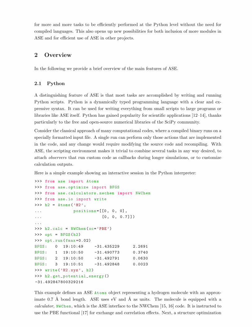
Here is a simple example showing an interactive session in the Python interpreter:

>>> from ase import Atoms

>>> from ase.optimize import BFGS

>>> from ase.calculators.nwchem import NWChem

>>> from ase.io import write

>>> h2 = Atoms(’H2’,

... positions =[[0, 0, 0],

... [0, 0, 0.7]])

...

>>> h2.calc = NWChem(xc=’PBE’)

>>> opt = BFGS(h2)

>>> opt.run(fmax =0.02)

BFGS: 0 19:10:49 -31.435229 2.2691

BFGS: 1 19:10:50 -31.490773 0.3740

BFGS: 2 19:10:50 -31.492791 0.0630

BFGS: 3 19:10:51 -31.492848 0.0023

>>> write(’H2.xyz’, h2)

>>> h2.get_potential_energy ()

-31.492847800329216

This example defines an ASE Atoms object representing a hydrogen molecule with an approx-

imate 0.7 A bond length. ASE uses eV and A as units. The molecule is equipped with a

calculator, NWChem, which is the ASE interface to the NWChem [15, 16] code. It is instructed to

use the PBE functional [17] for exchange and correlation effects. Next, a structure optimization

is performed using the BFGS [18] algorithm as implemented within ASE. The following lines of

output text show energy and maximum force for each iteration until it converges.

Note that due to dynamic typing, it is not necessary to declare the types of variables, and

due to automatic memory management, there are no explicit allocations or deallocations. This

makes the language clear and concise. However, Python itself is not designed for heavy nu-

merical computations. High-performance computational codes would need to be written in a

language that gives more control over memory, such as C or Fortran. Several Python libraries

are available which provide efficient implementations of numerical algorithms and other scientific

functionality. ASE relies on three external libraries:

• NumPy [8] provides a multidimensional array class with efficient implementations of basic

arithmetic and other common mathematical operations for ordinary dense arrays, such as

matrix multiplication, eigenvalue computation, and fast Fourier transforms.

• SciPy [19] works on top of NumPy and provides algorithms for more specialized numerical

operations such as integration, optimization, special mathematical functions, sparse arrays,

and spline interpolation.

• matplotlib [20] is a plotting library which can produce high-quality plots of many types.

Together, the three libraries provide an environment reminiscent of applications such as Octave

or Matlab.

It is also possible to write extensions in C that can be called from Python, or to link to com-

piled libraries written in another language. The DFT code GPAW [21, 22], which is designed

specifically to work with ASE, consists of about 85–90 % Python with the remainder written

in C. Almost all logically complex tasks are written in Python, whereas only computationally

demanding parts, typically tight loops of floating point operations, are written in C. Like most

DFT codes, GPAW also relies on external libraries such as BLAS and LAPACK for high per-

formance. ASE itself, however, does not perform extremely performance-critical functions and

is written entirely in Python.

2.2 Atoms and calculators

At the center of ASE is the Atoms object. It represents a collection of atoms of any chemical

species with given Cartesian positions. Depending on the type of simulation, the atoms may

have more properties such as velocities, masses, or magnetic moments. They may also have a

simulation cell given by three vectors and can represent crystals, surfaces, chains, or the gas

phase, by prescribing periodic or non-periodic boundary conditions along the directions of each

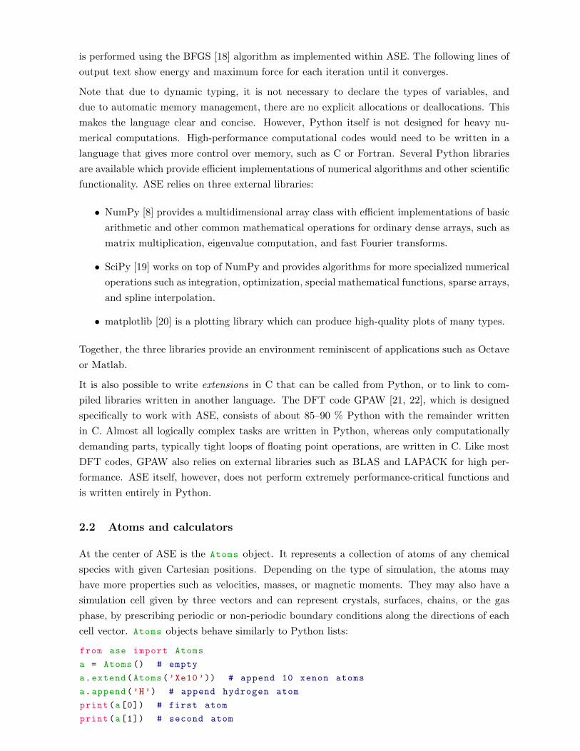
cell vector. Atoms objects behave similarly to Python lists:

from ase import Atoms

a = Atoms() # empty

a.extend(Atoms(’Xe10’)) # append 10 xenon atoms

a.append(’H’) # append hydrogen atom

print(a[0]) # first atom

print(a[1]) # second atom

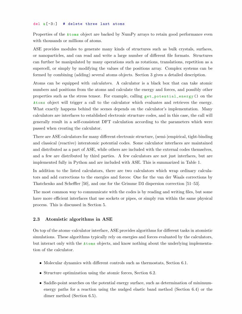
del a[-3:] # delete three last atoms

Properties of the Atoms object are backed by NumPy arrays to retain good performance even

with thousands or millions of atoms.

ASE provides modules to generate many kinds of structures such as bulk crystals, surfaces,

or nanoparticles, and can read and write a large number of different file formats. Structures

can further be manipulated by many operations such as rotations, translations, repetition as a

supercell, or simply by modifying the values of the positions array. Complex systems can be

formed by combining (adding) several atoms objects. Section 3 gives a detailed description.

Atoms can be equipped with calculators. A calculator is a black box that can take atomic

numbers and positions from the atoms and calculate the energy and forces, and possibly other

properties such as the stress tensor. For example, calling get_potential_energy () on the

Atoms object will trigger a call to the calculator which evaluates and retrieves the energy.

What exactly happens behind the scenes depends on the calculator’s implementation. Many

calculators are interfaces to established electronic structure codes, and in this case, the call will

generally result in a self-consistent DFT calculation according to the parameters which were

passed when creating the calculator.

There are ASE calculators for many different electronic structure, (semi-)empirical, tight-binding

and classical (reactive) interatomic potential codes. Some calculator interfaces are maintained

and distributed as a part of ASE, while others are included with the external codes themselves,

and a few are distributed by third parties. A few calculators are not just interfaces, but are

implemented fully in Python and are included with ASE. This is summarized in Table 1.

In addition to the listed calculators, there are two calculators which wrap ordinary calcula-

tors and add corrections to the energies and forces: One for the van der Waals corrections by

Tkatchenko and Scheffler [50], and one for the Grimme D3 dispersion correction [51–53].

The most common way to communicate with the codes is by reading and writing files, but some

have more efficient interfaces that use sockets or pipes, or simply run within the same physical

process. This is discussed in Section 5.

2.3 Atomistic algorithms in ASE

On top of the atoms–calculator interface, ASE provides algorithms for different tasks in atomistic

simulations. These algorithms typically rely on energies and forces evaluated by the calculators,

but interact only with the Atoms objects, and know nothing about the underlying implementa-

tion of the calculator.

• Molecular dynamics with different controls such as thermostats, Section 6.1.

• Structure optimization using the atomic forces, Section 6.2.

• Saddle-point searches on the potential energy surface, such as determination of minimum-

energy paths for a reaction using the nudged elastic band method (Section 6.4) or the

dimer method (Section 6.5).

Code Link Ref. Communication

Abinit http://www.abinit.org/ [23] Files

ASAPa https://wiki.fysik.dtu.dk/asap/ Python

Atomisticaa https://github.com/Atomistica/atomistica Python

Castep http://www.castep.org/ [24] Files

CP2K https://www.cp2k.org/ [25] Interprocess

deMon http://www.demon-software.com/ [26] Files

DFTB+ http://www.dftb-plus.info/ [27] Files

EAM Part of ASE [28] Python

ELK http://elk.sourceforge.net/ Files

EMT Part of ASE [29] Python

Exciting http://exciting-code.org/ [30] Files

FHI-aims https://aimsclub.fhi-berlin.mpg.de/ [31] Files

Fleur http://www.flapw.de/ [32] Files

Gaussian http://www.gaussian.com/ [33] Files

GPAWa https://wiki.fysik.dtu.dk/gpaw/ [22] Python

Gromacs http://www.gromacs.org/ [34] Files

Hotbita https://github.com/pekkosk/hotbit/ [35] Python

Dacapo https://wiki.fysik.dtu.dk/dacapo/ [7] Interprocess

JDFTxa https://sourceforge.net/projects/jdftx/ [36] Files

LAMMPS http://lammps.sandia.gov/ [37] Files

Lennard–Jones Part of ASE [38] Python

matscipya https://github.com/libAtoms/matscipy Python

MOPAC http://openmopac.net/ [39] Files

Morse Part of ASE [40] Python

NWChem http://www.nwchem-sw.org/ [41] Files

Octopus http://www.tddft.org/programs/octopus/ [42] Files

OpenKIMb https://openkim.org/ [43] Python

Quantum Espressoc http://www.quantum-espresso.org/ [44] Interprocess

QUIPa http://libatoms.github.io/QUIP/ [45] Python

SIESTA http://departments.icmab.es/leem/siesta/ [46] Files

TIP3P Part of ASE [47] Python

Turbomole http://www.turbomole.com/ [48] Files

VASP https://www.vasp.at/ [49] Files

aDistributed as part of the code instead of with ASEbDistributed by third party: https://github.com/mattbierbaum/openkim-kimcalculator-asecDistributed by third party: https://github.com/vossjo/ase-espresso

Table 1: Summary of ASE calculators.

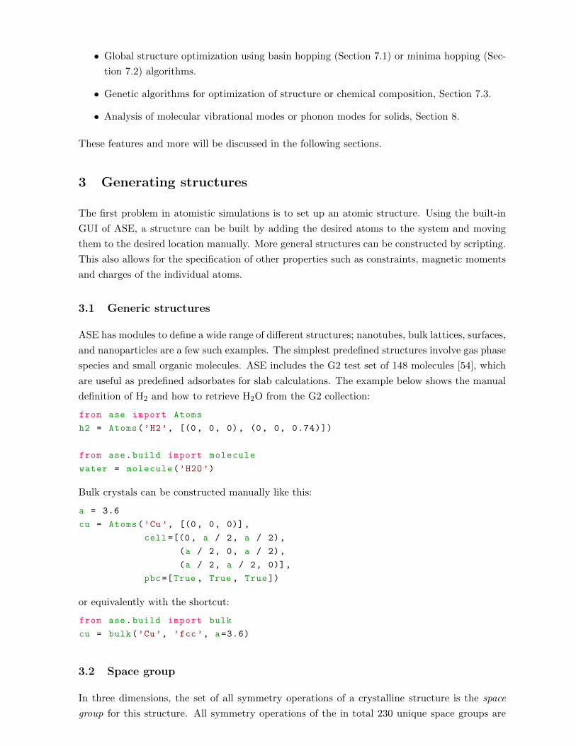
• Global structure optimization using basin hopping (Section 7.1) or minima hopping (Sec-

tion 7.2) algorithms.

• Genetic algorithms for optimization of structure or chemical composition, Section 7.3.

• Analysis of molecular vibrational modes or phonon modes for solids, Section 8.

These features and more will be discussed in the following sections.

3 Generating structures

The first problem in atomistic simulations is to set up an atomic structure. Using the built-in

GUI of ASE, a structure can be built by adding the desired atoms to the system and moving

them to the desired location manually. More general structures can be constructed by scripting.

This also allows for the specification of other properties such as constraints, magnetic moments

and charges of the individual atoms.

3.1 Generic structures

ASE has modules to define a wide range of different structures; nanotubes, bulk lattices, surfaces,

and nanoparticles are a few such examples. The simplest predefined structures involve gas phase

species and small organic molecules. ASE includes the G2 test set of 148 molecules [54], which

are useful as predefined adsorbates for slab calculations. The example below shows the manual

definition of H2 and how to retrieve H2O from the G2 collection:

from ase import Atoms

h2 = Atoms(’H2’, [(0, 0, 0), (0, 0, 0.74)])

from ase.build import molecule

water = molecule(’H2O’)

Bulk crystals can be constructed manually like this:

a = 3.6

cu = Atoms(’Cu’, [(0, 0, 0)],

cell =[(0, a / 2, a / 2),

(a / 2, 0, a / 2),

(a / 2, a / 2, 0)],

pbc=[True , True , True])

or equivalently with the shortcut:

from ase.build import bulk

cu = bulk(’Cu’, ’fcc’, a=3.6)

3.2 Space group

In three dimensions, the set of all symmetry operations of a crystalline structure is the space

group for this structure. All symmetry operations of the in total 230 unique space groups are

(a) (b)

Figure 1: (a) unit cell of beryl, (b) same cell repeated twice and seen along [001].

listed in the file spacegroup.dat in the ase.spacegroup package. The space group numbers

and nomenclature follow the definitions in International Tables [55].

The spacegroup package can create, and to some extent manipulate, crystalline structures. For

users of ASE, the most important function in this package is crystal () which returns a unit

cell of a crystalline structure given information about the space group, lattice parameters and

scaled coordinates of the non-equivalent atoms. The example below shows how to create a unit

cell of beryl§ from crystallographic information typically provided in publications:

from ase.spacegroup import crystal

# Adamo et al. Mineralogical Magazine 72 (2008) 799 -808

beryl = crystal(

symbols =[’Al’, ’Be’, ’Si’, ’O’, ’O’],

basis =[(2. / 3., 1. / 3., 0.25) , # Al

(0.5, 0.0, 0.25), # Be

(0.39 , 0.12, 0.00) , # Si

(0.50 , 0.15, 0.15) , # O1

(0.31 , 0.24, 0.00)] , # O2

spacegroup=’P 6/m c c’, # no 192

cellpar =[9.25 , 9.25, 9.22, 90, 90, 120])

The resulting structure is shown in Figure 1. The Spacegroup object can be used to investigate

symmetry-related properties of the structure, like whether beryl is centrosymmetric;

>>> from ase.spacegroup import Spacegroup

>>> sg = Spacegroup (192)

>>> sg.centrosymmetric

True

or to find its non-equivalent scaled atomic positions:

>>> sg.unique_sites(beryl.get_scaled_positions ())

array ([[ 0.33333333 , 0.66666667 , 0.25 ],

[ 0.5 , 0. , 0.25 ],

[ 0.88 , 0.27 , 0. ],

§Beryl is a naturally occurring mineral with chemical composition Be3Al2(SiO3)6 and a hexagonal crystal

structure with 58 atoms in the unit cell.

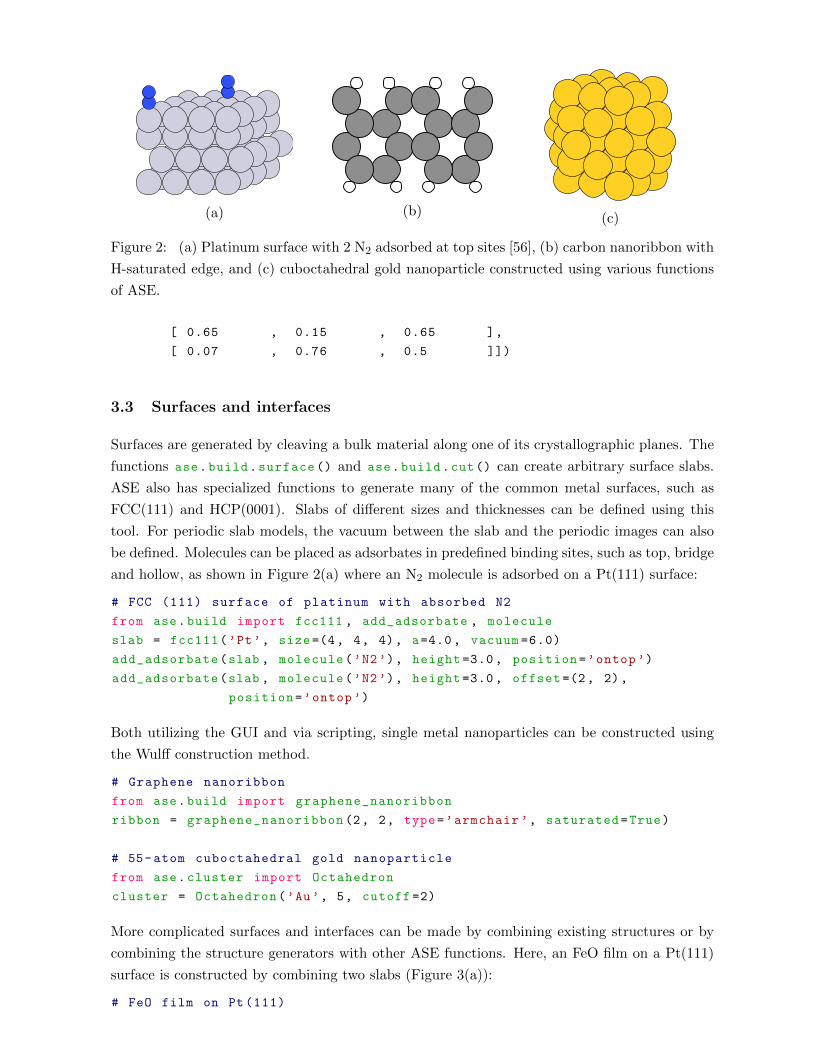
(a) (b)(c)

Figure 2: (a) Platinum surface with 2 N2 adsorbed at top sites [56], (b) carbon nanoribbon with

H-saturated edge, and (c) cuboctahedral gold nanoparticle constructed using various functions

of ASE.

[ 0.65 , 0.15 , 0.65 ],

[ 0.07 , 0.76 , 0.5 ]])

3.3 Surfaces and interfaces

Surfaces are generated by cleaving a bulk material along one of its crystallographic planes. The

functions ase.build.surface () and ase.build.cut() can create arbitrary surface slabs.

ASE also has specialized functions to generate many of the common metal surfaces, such as

FCC(111) and HCP(0001). Slabs of different sizes and thicknesses can be defined using this

tool. For periodic slab models, the vacuum between the slab and the periodic images can also

be defined. Molecules can be placed as adsorbates in predefined binding sites, such as top, bridge

and hollow, as shown in Figure 2(a) where an N2 molecule is adsorbed on a Pt(111) surface:

# FCC (111) surface of platinum with absorbed N2

from ase.build import fcc111 , add_adsorbate , molecule

slab = fcc111(’Pt’, size=(4, 4, 4), a=4.0, vacuum =6.0)

add_adsorbate(slab , molecule(’N2’), height =3.0, position=’ontop ’)

add_adsorbate(slab , molecule(’N2’), height =3.0, offset =(2, 2),

position=’ontop ’)

Both utilizing the GUI and via scripting, single metal nanoparticles can be constructed using

the Wulff construction method.

# Graphene nanoribbon

from ase.build import graphene_nanoribbon

ribbon = graphene_nanoribbon (2, 2, type=’armchair ’, saturated=True)

# 55-atom cuboctahedral gold nanoparticle

from ase.cluster import Octahedron

cluster = Octahedron(’Au’, 5, cutoff =2)

More complicated surfaces and interfaces can be made by combining existing structures or by

combining the structure generators with other ASE functions. Here, an FeO film on a Pt(111)

surface is constructed by combining two slabs (Figure 3(a)):

# FeO film on Pt (111)

(a) (b)

Figure 3: (a) Experimentally observed FeO film supported on Pt(111) substrate [57], (b) Pd

core/shell nanoparticle with Pt surface [58]

from ase.build import root_surface , fcc111 , stack

primitive_substrate = fcc111(’Pt’, size=(1, 1, 4), vacuum =2)

substrate = root_surface(primitive_substrate , 84)

primitive_film = fcc111(’Fe’, size=(1, 1, 2), a=3.9, vacuum =1)

primitive_film [1]. symbol = ’O’

film = root_surface(primitive_film , 67)

interface = stack(substrate , film , fix=0, maxstrain=None)

The neighbour list function provides the number and type of atoms in the vicinity of a given

atom and can therefore be used to find the coordination number of an atom. A Pd/Pt core/shell

nanoparticle can be constructed by utilizing the coordination number to identify surface atoms

(Figure 3(b)):

# Pt/Pd Core -Shell Nanoparticle

from ase.neighborlist import NeighborList

from ase.cluster import FaceCenteredCubic

atoms = FaceCenteredCubic(’Pd’, surfaces =[[1, 0, 0]], layers =[3])

nl = NeighborList ([1.4] * len(atoms), self_interaction=False ,

bothways=True)

nl.build(atoms)

for x, atom in enumerate(atoms):

indices , cell_offsets = nl.get_neighbors(x)

if len(indices) < 12:

atom.symbol = ’Pt’

4 Reading and writing structures

ASE presently recognizes 65 file formats for storing atomic configurations. Among these is the

simple xyz format, as well as many less well-known formats. ASE also provides two of its own

native file formats [59] in which all the items in an Atoms object – including momenta, masses,

constraints, and calculated properties such as the energy and forces – can be stored. The two

file formats are the compact traj format and a larger but human-readable json format. The

traj format is tightly integrated with other parts of ASE such at structure optimizers. A traj

file can contain one or more Atoms objects, but all of them must have the same number and

kind of atoms in the same order. The json file format can also contain more that one Atoms

object, but there are no restrictions on what it can contain (see also Section 4.1). Reading and

writing is done with the read() and write () functions from the ase.io module. The latter

can also be used to create images (png, svg, eps and pdf). It can also use POVRAY [60] to

render the output, like the core/shell nanoparticle on Figure 3(b).

4.1 Database

ASE has a database module (ase.db) that can be used for storing and retrieving atoms and

associated data in a compact and convenient way. A database for atomic configurations is ideal

for keeping systematic track of many related calculations. This will for example be the situation

in computational screening studies or when working with genetic search algorithms. Every row

in the database contains all the information stored in the atoms object and in addition key–value

pairs for storing extra quantities and for searching in the database.

Imagine a screening study looking for materials with a large density of states at the Fermi level.

Storing the results in a database could then look like this:

from ase.db import connect

connection = connect(’dos.db’)

for atoms in ...:

# Do calculation ...

dos = get_dos_at_fermi_level (...)

connection.write(atoms , dos=dos)

Here we have added a special dos column to our database, and we can now use the dos.db file

for analysis with either the ase.db Python module (connection.select(’dos >0.3’)) or

the ase-db command-line tool:

$ ase -db dos.db "dos >0.3"

The ase-db tool can also start a local web server so that one can query the database using a

web browser (see example in Figure 4). By clicking on a row of the table shown in the web

browser, one can see all the details for that row and also download the structure and data for

that row. There are currently three database backends:

JSON Simple human-readable text file.

SQLite3 Self-contained, serverless, zero-configuration database. SQLite3 is built into the

Python interpreter and the data is stored in a single file.

PostgreSQL Server-based database.

The JSON and SQLite3 backends work “out of the box”, whereas PostgreSQL requires a server.

4.2 Checkpointing

ASE includes a checkpointing module (ase.calculators.checkpoint) that adds powerful

generic restart and rollback capabilities to scripts. It stores the current state of the simulation

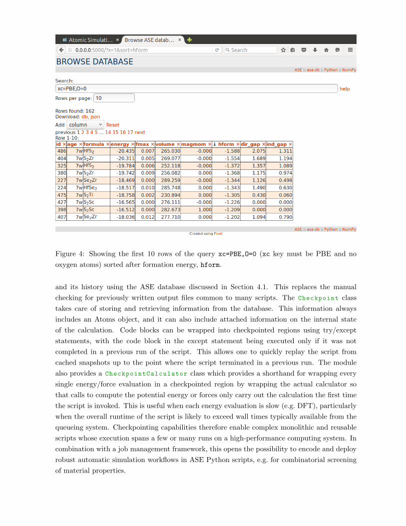
Figure 4: Showing the first 10 rows of the query xc=PBE,O=0 (xc key must be PBE and no

oxygen atoms) sorted after formation energy, hform.

and its history using the ASE database discussed in Section 4.1. This replaces the manual

checking for previously written output files common to many scripts. The Checkpoint class

takes care of storing and retrieving information from the database. This information always

includes an Atoms object, and it can also include attached information on the internal state

of the calculation. Code blocks can be wrapped into checkpointed regions using try/except

statements, with the code block in the except statement being executed only if it was not

completed in a previous run of the script. This allows one to quickly replay the script from

cached snapshots up to the point where the script terminated in a previous run. The module

also provides a CheckpointCalculator class which provides a shorthand for wrapping every

single energy/force evaluation in a checkpointed region by wrapping the actual calculator so

that calls to compute the potential energy or forces only carry out the calculation the first time

the script is invoked. This is useful when each energy evaluation is slow (e.g. DFT), particularly

when the overall runtime of the script is likely to exceed wall times typically available from the

queueing system. Checkpointing capabilities therefore enable complex monolithic and reusable

scripts whose execution spans a few or many runs on a high-performance computing system. In

combination with a job management framework, this opens the possibility to encode and deploy

robust automatic simulation workflows in ASE Python scripts, e.g. for combinatorial screening

of material properties.

5 Calculators

The calculator constitutes a central object in ASE and allows one to calculate various physical

quantities from an Atoms object. The properties that can be extracted from a given Atoms

object depend crucially on the nature of the calculator attached to the atoms. For example, a

DFT calculator may return properties such as the electronic density and Kohn–Sham eigenvalues,

which are inaccessible with calculators based on classical interatomic potentials.

5.1 Energy and forces

An important method common to every ASE calculator is get_potential_energy (), which

returns the potential energy of a given atomic configuration. In a quantum mechanical treatment

of the electrons, this is the adiabatic ground state energy of the electronic system. Applying the

method to two different atomic configurations will thus give the difference in energy between

the two configurations.

A useful application of the method is illustrated by the equation of state module exemplified by

the script below. The potential energy of fcc Al is calculated at various cell volumes and fitted

using the stabilized jellium model [61]. The fit is shown in Figure 5. This method provides a

convenient way of obtaining lattice constants for solids.

from ase.eos import EquationOfState

from ase.build import bulk

from gpaw import GPAW

from ase.calculators.emt import EMT

al = bulk(’Al’, crystalstructure=’fcc’, a=4.0)

calc = GPAW(mode=’pw’, kpts=(4, 4 ,4))

al.calc = calc

cell = al.get_cell ()

volumes = []

energies = []

for x in [0.9, 0.95, 1.0, 1.05, 1.1]:

al.set_cell(x * cell)

volumes.append(al.get_volume ())

energies.append(al.get_potential_energy ())

eos = EquationOfState(volumes , energies)

v0 , e0 , B = eos.fit()

eos.plot(’eos_Al.pdf’)

Another universal method carried by all calculators is get_forces (), which returns the forces

on all atoms. The method is applied extensively when performing dynamics or structure opti-

mization as described in Section 6.

10 12 14 16 18 20 22

volume [A3]

−4.2

−4.1

−4.0

−3.9

−3.8

−3.7

−3.6

−3.5

ener

gy[e

V]

sj: E: -4.130 eV, V: 15.906 A3, B: 85.511 GPa

Figure 5: Potential energy as a function of volume of bulk Al. A four-parameter fit is applied

to determine the optimal unit cell volume (V), energy (E) and bulk modulus (B).

5.2 Communication schemes

While calculators are black boxes from a scripting perspective, there are some differences in how

they interact with the environment. This section discusses how ASE deals with these technical

aspects. The following section discusses parallelization, which is essential for most applications.

ASE calculators can be classified by their interactions with the underlying simulation code. At

first, one can distinguish between calculators that run the simulation within the same Python

interpreter process and those that launch a separate sub-process.

Representatives for the first class are e.g. the GPAW and EMT calculators. (More listed in Ta-

ble 1 and denoted as “Python” for communication.) A big advantage of running the simulation

within the same process is zero-copy communication. The calculator can simply pass instan-

tiated ASE data-structures such as atoms.positions to the simulation code. In return, the

simulation code can write its atomic forces directly into the buffer of a NumPy array. Another

advantage is that it is easy for the calculator to store persistent information in memory that

survives across many similar consecutive calculations, e.g. in a molecular dynamics or geometry

optimization run. In those cases a significant speedup can be achieved by exploiting information

from the previous steps. For example, a DFT code can reuse the previous wave-function as an

initial guess for its next SCF optimization.

The second class of calculators execute the simulation code as a sub-process. (These are denoted

as “Interprocess” or “Files” in Table 1). This scheme is followed by the great majority of

ASE calculators. Most of these calculators communicate with their sub-process through the

filesystem. Hence, they generally perform the following four tasks:

1. The calculator generates an input file.

2. The calculator launches the simulation code as a sub-process.

3. The calculator waits for the sub-process to terminate.

4. The calculator parses the output files which were created by the simulation, and fills the

ASE data-structures.

The main advantage of this scheme is its simplicity. It interacts with the simulation code in the

same way as a user would. Hence, it does not require any changes to the simulation code itself.

The big disadvantage of this scheme is the high I/O costs. When there are many consecutive

invocations, a restart wave-function or electron density might have to be loaded from a file. If

the simulation is MPI-parallelized, then the binary has to be accessed by each compute node

before execution. Just creating the MPI session can already take several seconds [62].

Some file-based calculators like Quantum Espresso or Jacapo mitigate the start-up costs by

keeping the simulation process alive across multiple invocations. The next calculation is triggered

by writing a new input file, which the code automatically runs.

A way to avoid file I/O completely is to communicate via pipes. Such a scheme was recently

implemented by the CP2K calculator [25, 63]. For this, the CP2K distribution comes with a

small helper program called CP2K-shell. It provides a simple interactive command line interface

with a well defined, parseable syntax. When invoked, the CP2K calculator calls popen [64] to

launch the CP2K-shell as a sub-process and attaches pipes to its stdin and stdout file handles.

This even works together with MPI, because the majority of MPI-implementations forward the

stdin/stdout of the mpiexec process to the rank-0 process by default. The CP2K calculator

also allows for multiple CP2K instances to be controlled from within the same Python process

by instantiating multiple calculator objects simultaneously.

5.3 Parallel computing

Scientific computing is today usually done on computers with some kind of parallelism, either

multiple CPU cores in a single computer, or clusters of computers often with multiple cores

each. In the typical atomic-scale simulation performed with ASE, the performance bottleneck

is almost always the calculation of forces and energies by the calculator. For this reason, ASE

supports three different modes of calculator parallelization.

In the simplest case, a single process on a single core runs ASE, but whenever control is passed to

the calculator, the calculation runs in parallel. This is the natural model whenever the interface

to the calculator is file based: ASE writes the input files, starts the parallel calculation, and

harvests the result.

Another model, for example used by the GPAW calculator, is to have ASE running on each

CPU core with identical data. In this case Python itself is started in parallel e.g. by the mpiexec

tool. This is only used with calculators having a native Python interface written for ASE. One

has to be careful that all Python processes remain synchronized and with identical data. In this

way, the data from ASE is already present in the Python process on all cores, and any necessary

communication during the calculation is done by the calculator. Some care must be taken in

the user’s script when this model is used. First, data associated with the atoms must remain

identical on all processes. This is particularly an issue if random numbers are used, for example

in Monte Carlo simulations or Molecular Dynamics with the Langevin algorithm, where the

random numbers must be generated either by a deterministic pseudorandom number generator,

or on a single core and distributed to the rest. In most ASE modules using random numbers,

this is done automatically. Second, care must be taken when writing output files. If more than

one process writes to the same file, corruption is likely, in particular on network file systems.

Printing from just one process may be dangerous, since asking the atoms for any quantity

involving the calculator must be done on all processes to avoid a deadlock. ASE solves some of

these issues transparently by providing helper functions such as ase.parallel.paropen . This

function opens a file as normal on the master process, whereas data written by other processes

is discarded. Since the ASE data is not distributed, this is sufficient for any normal output and

does not require the user to think about parallelism.

For very large molecular dynamics simulations (millions of atoms), ASE is able to run in a

distributed atoms mode. Currently, only the Asap calculator is able to run in this mode, and

it needs to extend some modules normally provided by ASE. In this mode, the atoms are

distributed among the processes according to their position in space (domain decomposition),

each Python process thus only sees a fraction of the total number of atoms. If atoms move,

they need to be transferred between processes; for performance reasons this is the responsibility

of the calculator. When atoms thus migrate between processes, the number of atoms and

their identities change in each Python process. Any module that stores data about the atoms

internally, for example energy optimizers and molecular dynamics objects, will have their internal

data invalidated when this happens. For that reason, Asap needs to provide specialized versions

of such objects that delegate storage of internal data to the Atoms object. In the Atoms object,

all data is stored in a single dictionary, and the calculator then migrates all data from this

dictionary when atoms are transferred between processors.

When atomic configurations are written from a massively parallel molecular dynamics simula-

tion, all information is normally gathered in the master process before being written to disk

using one of ASE’s supported file formats. In the most extreme simulations, gathering all data

on the master process may be problematic (e.g. due to memory constraints). ASE supports a

special file format for handling this case: the BundleTrajectory . The BundleTrajectory

is not a file but a folder, with each atomic configuration in its own subfolder, and each quantity

in one or more files. Normally, data would be written by a single process, and each quantity is

written as an array into a single file, but in massively parallel simulations it is possible to have

each process write its own data into separate files. ASE then assembles the arrays when the

data is read again.

6 Dynamics and optimization

One is usually not only interested in static atomic structures, but also wants to study their

movement under internal and external influences. ASE provides multiple algorithms for structure

manipulation that can be used together with the calculator interfaces as was shown in the code

example in Section 2.1. The features supported by ASE and discussed in the following sections

are: molecular dynamics with different thermodynamic controls, searching for local and global

energy minima, or minimum-energy paths or transition states of chemical reactions. ASE further

allows these types of structure manipulations to be restricted by complex constraints.

6.1 Molecular dynamics

The general idea of molecular dynamics (MD) is to numerically solve Newton’s second law for

all the atoms, thus generating a time-series from an initial configuration. The purpose of the

molecular dynamics simulation may be to investigate the dynamics of a specific process, or to

generate an ensemble of configurations in order to calculate a thermodynamic property. Many

MD algorithms have been developed for related but slightly different purposes (see e.g. Ref. [65]).

This is reflected in the ASE code which supports a number of the more popular algorithms.

As Newton’s second law preserves the total energy of an isolated system, so will any algorithm

that integrates this equation of motion without modification: the simulation will produce a

microcanonical (or NV E) ensemble with well-defined particle number, volume and total energy.

One of the most popular such algorithms is velocity Verlet. In ASE this is implemented as a

dynamics object:

import ase.units

from ase.md.verlet import VelocityVerlet

dyn = VelocityVerlet(atoms , timestep =5 * ase.units.fs)

dyn.run (1000) # Run 1000 time steps

A dynamics object shares many of the properties of an optimization object; it is possible, for

example, to attach functions that are called at each time step, or after each N time steps.

Useful objects to attach this way include Trajectories for storing the atomic configuration and

MDLogger , which writes a log file with energies and temperatures.

6.1.1 Temperature control

Often, a constant-energy simulation is not what is desired, as the real system being modelled by

the simulation is thermally coupled to its surroundings, and thus has a well-defined temperature.

It is therefore necessary to be able to do simulations in the NV T ensemble without having to

describe the coupling to the surroundings in details. ASE implements three different algorithms

for constant-temperature MD: Berendsen dynamics, Langevin dynamics and Nose–Hoover dy-

namics.

Berendsen dynamics [66] is conceptually the simplest: at each time step the velocities

are rescaled such that the kinetic energy approaches the desired value over a characteristic

time chosen by the user. While simple, this algorithm suffers from the problem that the

magnitude of thermal fluctuations in the kinetic energy is not reproduced correctly, although

this is mainly a problem for very small systems. Berendsen dynamics can be found in the

ase.md.nvtberendsen module.

Langevin dynamics [67] adds a small friction and a fluctuating force to Newtons second law.

While originally invented to simulate Brownian motion, it can be argued to be a physically

reasonable approximation to the interactions with the electron gas in a metal. The main advan-

tages of Langevin dynamics are that it is very stable and that the thermostat is local : if kinetic

energy is produced in one part of the system, there is no risk that other parts cool down to

compensate, as can be the case with other thermostats. A possible drawback is that Langevin

dynamics is stochastic in nature, thus restarting a simulation will result in a slightly different

trajectory. Langevin dynamics is implemented in the ase.md.langevin module.

Nose–Hoover dynamics [68, 69] adds a single degree of freedom representing the heat bath;

this degree of freedom is coupled to the velocities of the atoms through a rescaling factor. This

method is very popular in the statistical mechanics community because it can be rigorously

derived from a Hamiltonian. One major drawback of this method is that with only a single

degree of freedom to describe the heat bath, oscillations may appear in this variable and thus in

the temperature. While Nose–Hoover dynamics is good at maintaining prescribed temperature,

it is therefore less suitable to establish a specific temperature in the simulation. This problem can

be addressed by introducing more auxiliary variables, the so-called Nose–Hoover chain, but this

is not implemented in ASE. Nose–Hoover dynamics is implemented together with Parrinello–

Rahman dynamics in the ase.md.npt module.

6.1.2 Pressure control

In addition to keeping temperature constant, it is often desirable to keep pressure (or the stress

for solids) constant, leading to the isothermal-isobaric (NpT ) ensemble. ASE provides two

algorithms for NpT dynamics: Berendsen and Nose–Hoover–Parrinello–Rahman.

Berendsen dynamics [66] allows for rescaling the simulation volume in addition to the kinetic

energy, leading to the conceptually simplest implementation of NpT dynamics. This algorithm

is implemented in the ase.md.nptberendsen module.

Nose–Hoover–Parrinello–Rahman dynamics is a combination of Nose–Hoover tempera-

ture control and Parrinello–Rahman pressure/stress control [70, 71]. ASE implements the al-

gorithm set forth by Melchionna [72, 73]. As is the case for Nose–Hoover dynamics, there is

the possibility of oscillations in the auxiliary variables controlling both the temperature and the

pressure, and the algorithm is more suitable for maintaining a given temperature and pressure

than for approaching it. The ASE implementation allows for varying only the volume of the

simulation box (suitable for constant-pressure simulations of e.g. liquids), and for varying both

shape and volume of the box, possibly constraining the simulation box to remain orthogonal. In

addition, constant strain rate simulations are possible where a dimension of the computational

box is kept unaffected by the dynamics, but is assigned a constant rate of change. This is

implemented in the ase.md.npt module.

6.2 Local structure optimizations

Local structure optimization algorithms start from an initial guess for the atomic positions and

(mostly) use the forces acting on the atoms to find structures of lower energy in an iterative

procedure until a given convergence criterion is reached. The methods available in ASE, in

ase.optimize , are described below.

BFGS (Broyden–Fletcher–Goldfarb–Shanno) [18, 74]. This algorithm chooses each step from

the current atomic forces and an approximation of the Hessian matrix, i.e. the matrix of second

derivatives of the energy with respect to the atomic positions (see Section 8.1). The Hessian is

established from an initial guess which is gradually improved as more forces are evaluated.

L-BFGS is a low-memory version of the BFGS algorithm [18, 75, 76]. The full Hessian matrix

has O(N2) elements, making BFGS very expensive for force field calculations with millions of

atoms. L-BFGS represents it implicitly as a series of up to n evaluated force vectors for a

linear-scaling memory requirement of O(nN).

MDMin is an energy minimization algorithm based on a molecular dynamics simulation. From

the initial positions, the atoms accelerate according to the forces acting on them. The algorithm

monitors the scalar product F·p of the force and momentum vectors. Whenever it is negative, the

atoms have started moving in an unfavourable direction, and the momentum is set to zero. The

simulation continues with whatever energy remains in the system. An advantage of MDMin

is that it is inspired by an intuitive physical process, but the algorithm does not converge

quadratically like those based on Newton’s method, and is therefore not efficient when close to

the minimum.

FIRE (fast inertial relaxation engine [77]) likewise formulates an optimization through molec-

ular dynamics. An artificial force term is added which “steers” the atoms gradually towards the

direction of steepest descent. FIRE uses a dynamic time step and other parameters to control

the simulation. Again, if at some point the atoms would move against the forces, the velocities

are set to zero and the dynamic parameters are reset. The FIRE algorithm often requires more

iterations than BFGS as implemented in ASE, but the atoms move in smaller steps which can

decrease the cost of a single self-consistent iteration.

SciOpt. ASE can use the optimization algorithms provided with SciPy for structure optimiza-

tions as well. However most of these general optimization algorithms are not as efficient as those

designed specifically for atomistic problems.

Preconditioners can speed up optimization approaches by incorporating information about

the local bonding topology into a redefined metric through a coordinate transformation. Pre-

conditioners are problem dependent, but the general-purpose implementation in ASE provides a

basis that can be adapted to achieve optimized performance for specific applications [78]. While

the approach is general, the implementation is specific to a given optimizer: currently L-BFGS

and FIRE can be preconditioned.

Tests with a variety of solid-state systems using both DFT and classical interatomic potentials

driven though ASE calculators show speedup factors of up to an order of magnitude for precon-

ditioned L-BFGS over standard L-BFGS, and the gain grows with system size. Precomputations

are performed to automatically estimate all parameters required. A line search based on enforc-

ing only the first Wolff condition (i.e. the Armijo sufficient descent condition) is also provided;

this typically leads to a further speed up when used in conjunction with the preconditioner.

The preconditioned L-BFGS method implemented in ASE does not require external depen-

dencies, but the scipy.sparse module can be used for efficient sparse linear algebra, and the

matscipy package is used for fast computation of neighbour lists if available. PyAMG can be used

to efficiently invert the preconditioner using an adaptive multigrid method.

6.3 Constraints

When performing optimization or molecular dynamics simulations one often wants to constrain

the movement of the atoms. For example, it is common to fix the lower layers of a “slab”-type

adsorbate–surface model to the bulk lattice coordinates. This can be achieved by attaching the

FixAtoms constraint to the atoms.

A number of built-in constraints are available in ASE. The user can easily combine these con-

straints or — if required — build their own constraints. The built-in constraints include:

• Fix atoms. Fixes the Cartesian positions of specified atoms.

• Fix bond length. Fixes a bond length between two atoms, while allowing the atoms to

otherwise move freely.

• Fixed-line, -plane, and -mode movement. An atom can be constrained to move only along

a specified line or within a specified plane; or, in fixed-mode, a system can be constrained

to move along a specified mode only. An example of fixed-mode could be a vibrational

mode.

• Preserving molecular identity. This constraint applies a restoring force if the distance

between two atoms exceeds a certain threshold. In this way molecules can be prevented

from dissociating. This class can also apply a restoring force to prevent an atom from

moving too far away from a specified point or plane. The constraint was designed to work

with techniques such as minima hopping in order to explore the potential energy surface

while enforcing molecular identity [79].

• Constraining internal coordinates. Any number of bond lengths, angles, and dihedral

angles can be constrained to fix the internal structure of a system.

An alternative to constraints is to use a “filter”, which works as a wrapper around the Atoms

object when it is used with a dynamics method (optimization, molecular dynamics etc.). In

other words, the dynamics sees only the degrees of freedom that the filter provides and not all

the atomic coordinates. The filter can thus hide certain degrees of freedom or make combinations

of them. A number of filters are built into ASE, and again the user is free to build their own.

The built-in methods include the following:

• Masking atoms. One can use a basic filter to fix the positions of specified atoms; this

works by presenting only the positions, forces, momenta, etc., on the free atoms when the

corresponding attributes are accessed. In particular for large-scale simulations, this can

have the advantage of reducing the size of the Hessian matrix.

• Optimizing unit cell vectors. A filter can present the stresses on the unit cell along with

the forces; this can be used to optimize the unit cell lattice vectors either simultaneously

or independently from the atomic positions. These filters also present the strain of the

unit cell as part of the positions attribute.

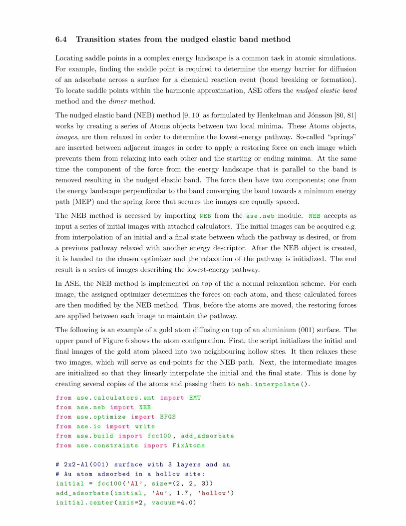
6.4 Transition states from the nudged elastic band method

Locating saddle points in a complex energy landscape is a common task in atomic simulations.

For example, finding the saddle point is required to determine the energy barrier for diffusion

of an adsorbate across a surface for a chemical reaction event (bond breaking or formation).

To locate saddle points within the harmonic approximation, ASE offers the nudged elastic band

method and the dimer method.

The nudged elastic band (NEB) method [9, 10] as formulated by Henkelman and Jonsson [80, 81]

works by creating a series of Atoms objects between two local minima. These Atoms objects,

images, are then relaxed in order to determine the lowest-energy pathway. So-called “springs”

are inserted between adjacent images in order to apply a restoring force on each image which

prevents them from relaxing into each other and the starting or ending minima. At the same

time the component of the force from the energy landscape that is parallel to the band is

removed resulting in the nudged elastic band. The force then have two components; one from

the energy landscape perpendicular to the band converging the band towards a minimum energy

path (MEP) and the spring force that secures the images are equally spaced.

The NEB method is accessed by importing NEB from the ase.neb module. NEB accepts as

input a series of initial images with attached calculators. The initial images can be acquired e.g.

from interpolation of an initial and a final state between which the pathway is desired, or from

a previous pathway relaxed with another energy descriptor. After the NEB object is created,

it is handed to the chosen optimizer and the relaxation of the pathway is initialized. The end

result is a series of images describing the lowest-energy pathway.

In ASE, the NEB method is implemented on top of the a normal relaxation scheme. For each

image, the assigned optimizer determines the forces on each atom, and these calculated forces

are then modified by the NEB method. Thus, before the atoms are moved, the restoring forces

are applied between each image to maintain the pathway.

The following is an example of a gold atom diffusing on top of an aluminium (001) surface. The

upper panel of Figure 6 shows the atom configuration. First, the script initializes the initial and

final images of the gold atom placed into two neighbouring hollow sites. It then relaxes these

two images, which will serve as end-points for the NEB path. Next, the intermediate images

are initialized so that they linearly interpolate the initial and the final state. This is done by

creating several copies of the atoms and passing them to neb.interpolate ().

from ase.calculators.emt import EMT

from ase.neb import NEB

from ase.optimize import BFGS

from ase.io import write

from ase.build import fcc100 , add_adsorbate

from ase.constraints import FixAtoms

# 2x2 -Al (001) surface with 3 layers and an

# Au atom adsorbed in a hollow site:

initial = fcc100(’Al’, size=(2, 2, 3))

add_adsorbate(initial , ’Au’, 1.7, ’hollow ’)

initial.center(axis=2, vacuum =4.0)

0.0 0.2 0.4 0.6 0.8 1.0

Normalized reaction coordinate

0.0

0.1

0.2

0.3

0.4

Pote

ntia

lene

rgy

(eV

)

0.37

Figure 6: The potential energy as a function of the normalized reaction path for the diffusion

path of a Au atom on the Al(001) surface.

# Fix second and third layers:

mask = [atom.tag > 1 for atom in initial]

initial.set_constraint(FixAtoms(mask=mask))

# Initial state:

initial.calc = EMT()

qn = BFGS(initial)

qn.run(fmax =0.05)

# Final state:

final = initial.copy()

final [-1].x += final.get_cell ()[0, 0] / 2

final.calc = EMT()

qn = BFGS(final)

qn.run(fmax =0.05)

images = [initial]

for i in range (3):

image = initial.copy()

image.calc = EMT()

images.append(image)

images.append(final)

# NEB object with new interpolated images

neb = NEB(images)

neb.interpolate ()

qn = BFGS(neb , trajectory=’neb.traj’)

qn.run(fmax =0.05)

write(’output.traj’, images)

The above script produces an output file containing the relaxed pathway used to produce Fig-

ure 6.

Finding the true saddle point for more complex pathways is not trivial. The best initial guess

for the reaction path may not be a linear interpolation between initial and final image, but

instead be related by rotations of subgroups of atoms. An improved preliminary guess for the

minimum energy path can be generated using images on the image dependent pair potential

(IDPP) surface [82]. Optimization of all atom pair distances toward an interpolation of all atom

pair distances for all intermediate images along the path results in an initial path much closer

to the MEP.

Once a good approximate reaction pathway has been determined, the climbing-image extension

of the NEB module can be invoked to converge the highest-energy image to the nearest saddle

point. The method works by omitting spring forces on the highest energy image and inverting

the force it experiences parallel to the path. The climbing image is still allowed to relax down the

energy landscape perpendicularly to the lowest-energy path like all other intermediate images.

Because the additional freedom of the climbing image makes this calculation computationally

more expensive, it is advised that this is only done when a good guess of the saddle point is

available.

Additional NEB extensions are available in the module. For instance, the full spring force is

omitted by default and only the spring force parallel to the local tangent is used together with

the true force (as evaluated by the calculator) perpendicular to the local tangent. A full list of

capabilities is available on the ASE website.

The standard NEB algorithm distributes the assigned computational resources equally to all the

images along the designated path. This implementation results in an inflexible and potentially

inefficient allocation of resources, given that each image has a different level of importance

towards finding the saddle point. A dynamic resource allocation approach is possible through

the AutoNEB [83] method in ase.autoneb . AutoNEB uses a simple strategy to add images

dynamically during the optimization.

AutoNEB first converges a rough reaction path with a few images using standard NEB. Once

converged, an image is added either where the gap between the current images is largest, or

where the energy slope is greatest. The reaction path is refined by iteratively adding images

and reconverging the pathway.

The virtue of the AutoNEB method is that it is possible to define a total number of internal

images which is greater than the number of images to simultaneously participate in the optimi-

sation. Some images will then be moving while others are frozen. Whenever an image is added,

the moving images will be those closest to the most recently added one. This feature allows

for computational resources to always be focused on the most important region of the pathway.

The method has been utilized for a number of examples [84–86] with benchmarking cases with

50–70% reduced computational cost relative to the standard algorithm [86].

For systems with no fixed atom positions and/or periodic boundary conditions, overall rota-

tion and translation are external changes with no internal structural changes. For normal NEB

calculations involving nanoparticles, external structural changes can pose problems for the con-

vergence to the minimum energy path. The system will seek to avoid high energy areas and

hence rotate and/or translate away from these, which is not possible to the same extent for

a constrained system. The NEB module supports the NEB-TR [87] method, which speeds up

convergence for such systems by removing rotation and translation movement.

6.5 Transition states from the dimer method

Like the NEB method above, the dimer method is used to find saddle points in multidimensional

potential energy landscapes. Unlike NEB, the dimer method only requires a starting basin and

is useful for finding most or all relevant pathways out of that basin.

The dimer method is a minimum mode following method which estimates the eigenmode corre-

sponding to the lowest eigenvalue of the Hessian (minimum mode) and traverses the potential

energy surface (PES) uphill in that direction. Eventually, it reaches a first order saddle point

with exactly one negative eigenvalue.

The dimer method can be split into three independent phases.

1. Estimating the minimum mode.

2. Inverting the gradient along the minimum mode to make first order saddle points appear

as minima.

3. Move the system according to the inverted gradient.

Only the first of these phases is unique to the dimer algorithm. Other methods estimate the

minimum mode differently. The dimer method is implemented in ASE in such a way that it

should be straightforward to include other minimum mode estimators.

To find a saddle point, the system is initially located at an energy minimum and randomly

displaced [88]. The displacement achieves two things: first, it moves the system away from a

zero gradient location (the minimum), and secondly, it can be used as the seed to sample as

many saddle points as possible.

The dimer method identifies the minimum mode by making an estimate of the curvature of

the PES along a given unit vector, s, and then iteratively rotates s until it reaches an energy

minimum. This energy minimum represents the lowest curvature.

The name of the dimer method is derived from the way that s is defined. Two images are chosen:

one with the input system coordinates and the other displaced along s by a distance of ∆D.

The gradients at each image are then used to estimate the 2nd derivative of the PES using finite

difference. The force components perpendicular to s are used to determine the torque which

rotates the dimer to obtain lower energy, iteratively reaching the estimate of the minimum mode.

The dimer method is implemented in ASE through the DimerAtoms class, which extends the

Atoms class with information relevant to the dimer method, such as the minimum mode estimate

and the curvature. The system can initially be displaced from the energy minimum configuration

by a predefined vector, by selecting certain atoms to be randomly displaced or by defining a

sphere in which all atoms are randomly displaced.

A default dimer calculation can be set up by creating a DimerAtoms object from an Atoms ob-

ject with a calculator attached. The parameters controlling the calculation can either be passed

directly to the DimerAtoms object when created or can be specified using a DimerControl

object.

Multiple control parameters are defined in the DimerControl but the most important ones

have to do with ∆D and the amount of rotations allowed before performing an optimization

step:

• Rotational force thresholds to define the conditions under which no more rotations will be

performed before performing an optimization step.

• The maximum number of rotations to be performed before making an optimization step.

• ∆D, the separation of the dimer’s images. In order for an accurate finite difference estimate

of the 2nd derivative, this should be kept small, but still large enough to avoid effects of

noise in the force calculations.

7 Global optimization

Finding the atomic configuration with the lowest possible energy is much more challenging than

finding just a local minimum. The number of local minima grows at least exponentially with the

number of atoms (the existence of about 106 local minima for a 147-atom Lennard-Jones cluster

has been suggested [89]), and finding the global minimum is therefore a daunting task. One of

the main challenges for global optimization is that different local minima might be separated by

high energy barriers which much be overcome in order to move between local minima.

One common approach to this problem is simulated annealing, in which the atomic system is

initially equilibrated at a certain temperature using, for example, molecular dynamics. After

this, the temperature is decreased slowly to identify low energy configurations. However, this

method is not always efficient and a number of alternative global optimization techniques have

been developed.

ASE provides three methods for global optimization: basin hopping, minima hopping and genetic

algorithms.

7.1 Basin hopping

In the basin hopping method [89], the atoms perform a random walk. Every structure visited

is relaxed with a local optimization method, and the unrelaxed structure is then assigned the

energy of the obtained minimum. Thus all structures within the same basin are considered to

have the same energy. In this way the barriers between close-lying local minima are effectively

removed, and the PES becomes a step-function with the energies defined by the local minima

(see the illustrative Figure 2 in Ref. [89]). The modified PES is then explored by Monte Carlo at

an adjustable temperature: Going from one basin to another is accepted at random depending

on how favourable its energy is.

7.2 Minima hopping

A more automated approach is minima hopping [90], in which one uses alternating MD and

local minimization steps in combination with self-adjusting parameters to explore the potential

energy surface. Briefly, a MD step at a specified initial temperature is used to randomly “shoot”

the structure out of a local minimum region in the PES; after the MD trajectory encounters a

specified number of path minima, the structure is optimized to the next local minimum. If the

minimum found is identical to any previously-found minimum, the MD temperature is increased

and the step is repeated. Otherwise the algorithm first lowers the search temperature and then

decides to accept the step if the new local minimum is no higher than a specified energy difference

above the previous step. If the found local minimum is accepted, it is added to a list of found

minima and the energy difference threshold is decreased. If it is rejected, the energy difference

threshold is increased. In this way, a list of local minima is generated while two parameters—

the search temperature and the acceptance criterion—are automatically adjusted in response

to the success of the algorithm. The ASE implementation of minima hopping allows the user

to easily customize the key features of the algorithm, such as the local optimizer employed or

the molecular dynamics scheme. It is also possible to perform parallel searches which share the

list of found minima. The minima hopping scheme can also be combined with constraints, for

example to prevent molecules from dissociating [79].

7.3 Genetic Algorithms

In addition to the global optimization schemes described in Sections 7.1 and 7.2, ASE also

contains ase.ga, a genetic algorithm [91–94] (GA) module. A GA takes a Darwinistic approach

to optimization by maintaining a population of solution candidates to a problem (e.g. what is the

most stable four component alloy [95]?). The population is evolved to obtain better solutions

by mating and mutating selected candidates and putting the fittest offspring in the population.

The fitness of a candidate is a function which, for example, measures the stability or performance

of a candidate. Natural selection is used to keep a constant population size by removing the

least fit candidates. Mating or crossover combine candidates to create offspring with parts from

more candidates present, when favorable traits are combined and passed on the population is

evolved. Only performing crossover operations risks stagnating the evolution due to a lack of

diversity – performing crossover on very similar candidates is unlikely to create progress when

performed repeatedly. Mutation induces diversity in the population and thus prevents premature

convergence.

GAs are generally applicable to areas where traditional optimization by derivative methods are

unsuited and a brute force approach is computationally infeasible. Furthermore, the output

of a GA run will be a selection of optimized candidates, which often will be preferred over

only getting the best candidate, especially taking into account the potential inaccuracy of the

employed methods. Thus a GA finds many applications within atomic simulations, and will

often be one of the best methods for searching large phase spaces. We will present a couple of

usage cases in Section 7.3.1.

7.3.1 Usage examples of the GA implementation in ASE

The ase.ga implementation has been used to determine the most stable atomic distribution

in alloy nanoparticle catalysts [96, 97]. For this purpose, specific permutation operators were

implemented promoting the search for different possible atomic distributions within particles,

i.e. core/shell, mixed or segregated. For example the operator promoting core/shell particles

permutes two atoms in the central and surface region respectively, a mixed (segregated) particle

is promoted by permuting two atoms each in local environments with a high (low) density of

identical atoms. These operators, if used dynamically, greatly improved the convergence speed

of the algorithm.

The most stable Au6–12 clusters on a TiO2 support were also determined using ase.ga [98]. The

approach, inspired by Deaven and Ho [99], implemented the cut-and-splice operator and utilized

the flexibility of ASE to perform local optimization with increasing levels of theory. This led to

the discovery of a new global minimum structure. The GA implementation was benchmarked

for small clusters and described in greater detail in [100].

Bulk systems are also readily treated in ase.ga; for example, ase.ga was used in a search

for ammonia storage materials with high storage capacities and optimal ammonia release char-

acteristics. The best candidates, some with a record high accessible hydrogen capacity, were

subsequently experimentally verified [101, 102]. Operators utilizing chemical trends were imple-

mented, e.g. mutating an atom to a neighboring element in the periodic table (up, down, right

or left). This approach is readily transferable to other screening studies where the phase space

is too great for a full computational screening.

7.3.2 GA implementation in ASE

The implementation requires some insight from the user on how the algorithm should treat the

problem, e.g. which operators are appropriate or when is convergence achieved. The only way to

get the algorithm running optimally is by testing the use of different functions and parameters

for the given search objective. However, even without optimization of parameters, the GA

can perform reasonably well. In the following we shall discuss the different components in a

GA calculation in ASE (also shown in the flow chart Figure 7), and provide an example for

optimization of a small cluster on a gold surface. Other GA examples are available on the ASE

web-pages.

Start The initial population must be generated to start. A helper function, StartGenerator ,

is supplied for atomic clusters. The initial population can be random (unbiased) or com-

prise seeded suggestions, e.g. candidates the user thinks will be good (biased). The subse-

quent steps are then repeated until some convergence criterion is reached.

Store Unevaluated candidates (initial or offspring) are saved in the database.

StartStartGenerator

Storease.db

Evaluateset_raw_score

Storease.db

PopulationPopulation

OperationCrossover

and/or Mutation

Selectionget_two_candidates

Stop?Convergence

The end!

no

yes

Figure 7: Flow of the genetic algorithm. Examples of functions or classes at each step are shown

in green.

Evaluate Candidates are typically evaluated in a separate script, allowing the search to progress

in parallel through a queueing system. The evaluation will typically involve a local geome-

try optimization. The main objective of the evaluation script is to calculate the raw score,

i.e. the fitness of the candidate without taking the rest of the population into account.

Evaluated candidates and their raw scores are added to the database.

Population The population step determines how to calculate the fitness from the raw score.

It is useful to compare candidates collectively and only keep the fittest one of similar

candidates. This can also be achieved by penalizing the fitness of similar candidates.

Stop The GA run is normally considered converged when no evolution of the fittest candidates

takes place for a certain amount of time. It is also possible to set a hard limit for the

number of candidates that should be generated and conclude the search once this criterion

has been met.

Selection This step performs the selection among the current population, e.g. by the roulette

wheel method. This can function in two ways:

1. Generational where the current population is used as parents to form a new generation

of candidate offspring. The new generation and current population are then combined

to form the new population. However, since the algorithm halts until the evaluation

of a full generation is finished, this does not parallelize optimally.

2. The population can be treated as a pool from which candidates are used as parents

and to which new candidates are added continually. This keeps the computational

load constant.

Operation The types of operators to use in a search are determined by the specific problem.

It is always desirable though to use both crossover and mutation, however not necessarily

in equal amounts – it is possible to give a certain weight to any operator, that can be

changed dynamically [96]. It should be noted that, for a problem well suited to a GA, it

will be beneficial to set a greater likelihood of crossover compared to mutation. The newly

created offspring is added to the database and the whole cycle repeats.

If the user has a new idea, the easiest way to implement it is to modify a copy of one of the

existing classes.

Once the GA script runs, no action is required from the user, but it is beneficial to check the

evolution by investigating the db file as described in section 4.1. It is typical to run a GA

several times with identical or slightly different initial conditions to verify the global minimum.

If allowed by the nature of the problem, it is common to utilize a central database to check

during the evaluation step if the candidate has been calculated in a previous run or in another

instance of the GA running in parallel.

7.3.3 Running a genetic algorithm

In the following we outline a complete GA search for maximally stable configurations of a

gold/silver overlayer on top of a 2×4×1 Au(111) slab The complete code for the example can

be found on the ASE web page.

First, the gold slab is created. A random initial population is then produced on top of the

slab (as displayed in Figure 8a) and added to the database using the two ase.ga objects

StartGenerator and PrepareDB . The start population is subsequently relaxed before the

GA run is initiated. Examples from an unrelaxed start population can be found in Figures 8b,

c, and d.

The next step is to set up the population, pairing scheme, and types of mutation before the

population is evolved. This is facilitated by helper classes for cut-and-splice pairing and per-

mutation mutations. In this case, 50 new candidates are initialized either by mutation (30 %

permutation mutation in this case) or by a crossover pairing of two candidates from the current

population. New candidates are relaxed in turn while keeping the population updated with

the fittest 20 unique candidates after each new child is added to the database. Setting up the

population and running the main loop can be done as shown in the code example below.

# Create the population

n_to_optimize = len(atom_numbers)

comp = InteratomicDistanceComparator(n_top=n_to_optimize)

population = Population(data_connection=da, population_size =20,

comparator=comp)

pairing = CutAndSplicePairing(slab , n_to_optimize , blmin)

mutation = PermutationMutation(n_to_optimize)

# Test 50 new candidates

for i in range (50):

parent1 , parent2 = population.get_two_candidates ()

# Check if we want to do a mutation (30 % chance) or pair candidates

if random () < 0.3:

child , desc = mutation.get_new_individual ([ parent1 ])

else:

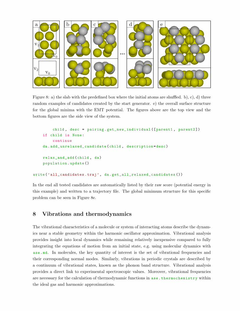
b c eda

v0

v1

v2 v0

Figure 8: a) the slab with the predefined box where the initial atoms are shuffled. b), c), d) three

random examples of candidates created by the start generator. e) the overall surface structure

for the global minima with the EMT potential. The figures above are the top view and the

bottom figures are the side view of the system.

child , desc = pairing.get_new_individual ([parent1 , parent2 ])

if child is None:

continue

da.add_unrelaxed_candidate(child , description=desc)

relax_and_add(child , da)

population.update ()

write(’all_candidates.traj’, da.get_all_relaxed_candidates ())

In the end all tested candidates are automatically listed by their raw score (potential energy in

this example) and written to a trajectory file. The global minimum structure for this specific

problem can be seen in Figure 8e.

8 Vibrations and thermodynamics

The vibrational characteristics of a molecule or system of interacting atoms describe the dynam-

ics near a stable geometry within the harmonic oscillator approximation. Vibrational analysis

provides insight into local dynamics while remaining relatively inexpensive compared to fully

integrating the equations of motion from an initial state, e.g. using molecular dynamics with

ase.md. In molecules, the key quantity of interest is the set of vibrational frequencies and

their corresponding normal modes. Similarly, vibrations in periodic crystals are described by

a continuum of vibrational states, known as the phonon band structure. Vibrational analysis

provides a direct link to experimental spectroscopic values. Moreover, vibrational frequencies

are necessary for the calculation of thermodynamic functions in ase.thermochemistry within

the ideal gas and harmonic approximations.

8.1 Molecular vibrations

We begin by expanding the potential energy function with respect to atomic positions, ui:

E = E0 +3N∑i

∂E

∂ui

∣∣∣∣0

(ui − ui0) +1

2

3N∑i

3N∑j

∂2E

∂ui∂uj

∣∣∣∣0

(ui − ui0)(uj − uj0) + · · · (1)

Here, indices i and j run over the three coordinate axes of N atoms and the subscript 0 indicates

the reference geometry. The first term in the expansion accounts for an arbitrary shift of the

total potential energy, so we are free to set it equal to zero. Assuming the expansion is about

a stationary point on the potential energy surface (usually energy minima and occasionally

saddle points are of interest), the derivative in the linear term of the expansion is zero. Ignoring

higher-order terms, we may rewrite the expansion as

E =1

2

∑i,j

∆uiHij∆uj =1

2∆uTH∆u. (2)

H is called the Hessian matrix and is defined as

Hij =∂2E

∂ui∂uj

∣∣∣∣0

= −∂Fj∂ui

. (3)

In the above expression, Fj denotes the force along the atomic coordinate axis j. H is constructed

from finite-difference first derivatives of the forces obtained from an attached ASE calculator.

Each atom is displaced forwards and backwards along each coordinate axis, requiring 6N+1 total

force evaluations. Note that, by construction, H is symmetric. It follows that the eigenvalues of

H are real and its eigenvectors form a complete orthogonal basis. Writing Newton’s equations

of motion in terms of the Hessian yields

−H∆u = Md2∆u

dt2, (4)

which is solved by uk(t) = akexp(−iωkt). Plugging in this solution, the equation of motion

becomes

Huk = ω2kMuk, (5)

where M is a diagonal matrix of the atomic masses. This is then solved as a standard eigen-

value problem. The eigenvalues of the mass-weighted Hessian M−1/2HM−1/2 are the squared

vibrational frequencies and the eigenvectors are the mass-weighted normal modes M1/2uk.

Many calculators represent quantities such as the electron density on a real-space grid. This

gives rise to the so-called egg-box effect: The forces on each atom vary artificially under trans-

lational movement of the grid relative to the atom, leading to inaccuracies in the Hessian. This

dilemma may be resolved for isolated systems by imposing momentum conservation [103] such

that∑

iHij = 0 for all j. In ASE, this condition is enforced by adjusting the diagonal elements

through Hjj = −∑i 6=j Hij , which preserves the symmetry of H.

The effect is to replace the force on an atom when displaced from its equilibrium position with

minus the sum of the forces on all other atoms under the same displacement, averaging the

egg-box noise over the whole system.

In practice, the vibrations of a molecule described by an Atoms object is found by creating a

Vibrations object and running it:

from ase.vibrations import Vibrations

vib = Vibrations(atoms)

vib.run()

The Vibrations object can then be queried for information about the calculated vibrational

modes.

8.2 Spectral properties

Post-processing methods are available in ase.vibrations for calculating spectral properties

related to vibrations. These methods use quantities that are calculated via finite difference

displacements. Infrared spectra can be obtained from changes in molecular dipoles [104] that

are available from electronic structure calculators.

Raman spectra are more involved, as they require excited state properties that are not as

commonly provided by calculators as ground state properties. The ASE modules are intended

to be usable with different caculators, but were tested so far with GPAW only. These modules

are a work in progress, but special topics like the evaluation of approximate Raman spectra [105]

and the calculation of Franck–Condon overlaps depending on Huang–Rhys factors derived from

excited state forces already exist.

8.3 Phonons

Treatment of lattice dynamics in terms of phonons is essential for describing many properties of

crystalline solids including thermodynamic functions (see ase.thermochemistry), supercon-

ductivity, infrared and Raman absorption, phase transitions and sound propagation [106]. The

ase.phonons module is used to calculate phonon frequencies, which can be used to construct

band structures and densities of states and visualize the time-dependent motion of the phonon

modes.

The calculation of phonon modes may be thought of as an extension of the vibrational analysis

described in Section 8.1 to a periodic lattice. The phonon modes are characterized by a wave

vector k, which specifies the direction and spatial frequency of propagation.

Two well-established ab initio methodologies for performing phonon analyses are the finite dis-

placement method, also called the direct method [107], and the linear response method [108].

ase.phonons uses the former, in which the primitive cell is repeated across its periodic bound-

ary conditions to form a supercell. Ideally, the supercell should be large enough that no atom

interacts with any of its periodic images in neighboring cells. In ordinary metals, interatomic

forces decay rapidly. In polar materials, the dipole–dipole forces are longer in range. For reliable

results one should therefore always check any phonon-related observable for convergence with

respect to supercell size.

The matrix of force constants, H, is calculated by displacing the atom or atoms in one primitive

cell within the supercell along each Cartesian axis and calculating the force response on all other

atoms in the supercell. It is only necessary to perform the displacement on the atoms in this one

dynamic primitive cell because all other primitive cells in the crystal are related by translation of

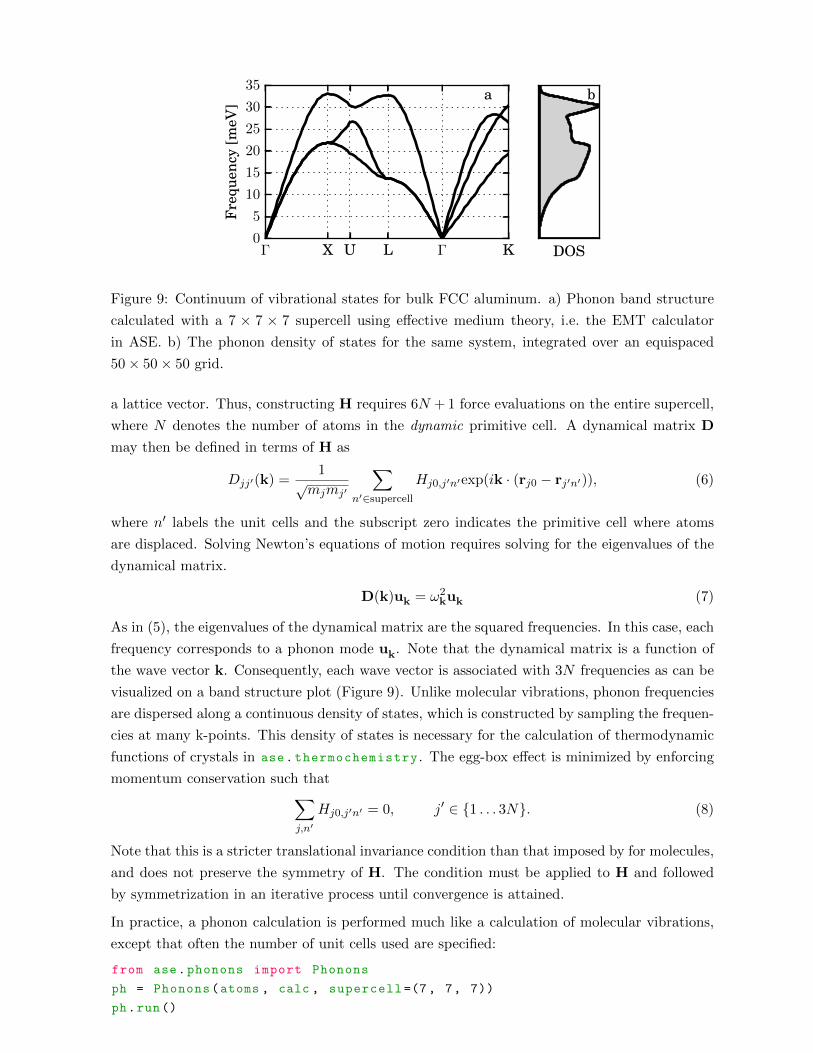
Γ X U L Γ K0

5

10

15

20

25

30

35

Fre

quen

cy[m

eV]

a

DOS

b

Figure 9: Continuum of vibrational states for bulk FCC aluminum. a) Phonon band structure

calculated with a 7 × 7 × 7 supercell using effective medium theory, i.e. the EMT calculator

in ASE. b) The phonon density of states for the same system, integrated over an equispaced

50× 50× 50 grid.

a lattice vector. Thus, constructing H requires 6N + 1 force evaluations on the entire supercell,

where N denotes the number of atoms in the dynamic primitive cell. A dynamical matrix D

may then be defined in terms of H as

Djj′(k) =1

√mjmj′

∑n′∈supercell

Hj0,j′n′exp(ik · (rj0 − rj′n′)), (6)

where n′ labels the unit cells and the subscript zero indicates the primitive cell where atoms

are displaced. Solving Newton’s equations of motion requires solving for the eigenvalues of the

dynamical matrix.

D(k)uk = ω2kuk (7)

As in (5), the eigenvalues of the dynamical matrix are the squared frequencies. In this case, each

frequency corresponds to a phonon mode uk. Note that the dynamical matrix is a function of

the wave vector k. Consequently, each wave vector is associated with 3N frequencies as can be

visualized on a band structure plot (Figure 9). Unlike molecular vibrations, phonon frequencies

are dispersed along a continuous density of states, which is constructed by sampling the frequen-

cies at many k-points. This density of states is necessary for the calculation of thermodynamic

functions of crystals in ase.thermochemistry . The egg-box effect is minimized by enforcing

momentum conservation such that∑j,n′

Hj0,j′n′ = 0, j′ ∈ {1 . . . 3N}. (8)

Note that this is a stricter translational invariance condition than that imposed by for molecules,

and does not preserve the symmetry of H. The condition must be applied to H and followed

by symmetrization in an iterative process until convergence is attained.

In practice, a phonon calculation is performed much like a calculation of molecular vibrations,

except that often the number of unit cells used are specified:

from ase.phonons import Phonons

ph = Phonons(atoms , calc , supercell =(7, 7, 7))

ph.run()

The Phonons object can then be queried for information about the different phonon modes.

8.4 Thermochemistry

A common task in atomistic simulations is to convert the output of electronic structure cal-

culations, which represent calculations of single configurations on the potential energy surface

(PES), into thermodynamic properties, which are statistical functions of the energetics over an

ensemble of states. For example, optimization routines within ASE can find a local minimum

on the PES; however, to convert this potential energy Epot into a thermodynamic quantity such

as the free energy, a statistical-mechanics treatment that utilizes the shape of the PES near

the local minimum is necessary, along with an appropriate model. Three standard cases are

implemented in ASE (within ase.thermochemistry) to convert PES information into ther-

modynamic quantities (ignoring electronic excitation contributions to the heat capacity); given

the modular nature of ASE, the user can readily expand upon these basic methods with cus-

tomized methods as needed, for example to deal with anharmonicity or electronic contributions.

The three standard approaches are listed below.

• The harmonic limit. In the simplest case, all 3N atomic degrees of freedom (DOFs)

are treated as separable and harmonic within the accessible temperature range; the vibra-

tional energy levels εi corresponding to these motions can be produced from a normal-mode

analysis as described in Section 8.1. This is the same treatment as in the ideal-gas limit,

described below, but without translational or vibrational DOFs. A common example of

this limit is the examination of the thermodynamics of an adsorbed species on a catalytic

surface [109]; the 3N DOFs of the adsorbate are then assumed to be harmonic and in-

dependent of the modes in the surface. This allows the calculation of properties such as

internal energy U and entropy S at a specified temperature T with the Helmholtz energy

F = U − TS. These methods are available via the HarmonicThermo class. The internal

energy is taken to be

U(T ) = Epot + ∆EZPE +3N∑i

εi

eεi/kBT − 1, (9)

where the zero-point energy ∆EZPE has its usual definition of 12

∑i εi and kB is the Boltz-

mann constant. The entropy is found from

S(T ) = kB

3N∑i

[εi

kBT(eεi/kBT − 1

) − ln(

1− e−εi/kBT)]

. (10)

• The ideal-gas limit. In the limit of an ideal gas, one assumes that the 3N atomic DOFs

can be treated independently and separated into translational, rotational, and vibrational

components [110, 111]. Three-dimensional gases have three translational DOFs. General

polyatomic gases have an additional three rotational DOFs; although linear molecules

have only two rotational DOFs and monotonic gases have none. The remaining DOFs are

vibrations which are treated harmonically in this limit. This allows for the calculation

of such properties as the enthalpy H, entropy S, and Gibbs free energy G. Aside from

ideal gases, this method can be used to estimate the properties of condensed species via

thermodynamic arguments. For example, the direct calculation of the free energy of liquid

water at 298 K from first principles is daunting. However, one can calculate the free energy

of water vapor in equilibrium with liquid water (which, at a vapor pressure of 3.2 kPa is

well described by the ideal-gas approximation), and equate this to the free energy of liquid

water via the thermodynamic criterion for equilibrium. These methods are available in

the IdealGasThermo class. The enthalpy is calculated as

H(T ) = Epot + ∆EZPE +

∫ T

0CP dT, (11)

where the constant-pressure heat capacity is

CP = kB + CV ,trans + CV ,rot + CV ,vib. (12)

The translational heat capacity term is 32kB, while the rotational term is 1

2kB per rotational

DOF. The integral of the vibrational heat capacity takes the same form as in (9), with the

sum taken over the vibrational DOFs. The entropy is found from

S(T, P ) = S◦trans + Srot + Svib + Selec − kB lnP

P ◦, (13)

where the translational term is calculated at a reference pressure P ◦. The vibrational

component is the same as (10) whereas the remaining components are given below.

Strans = kB

{ln

[(2πMkBT

h2

)3/2 kBT

P ◦

]+

5

2

}, (14)

Srot =

0 if monatomic,

kB

[ln(8π2IkBTσh2

)+ 1]

if linear,

kB

{ln

[√πIAIBICσ

(8π2kBTh2

)3/2]+ 3

2

}if nonlinear,

(15)

Selec = kB ln [2× (spin multiplicity) + 1] . (16)

In the above, IA, IB, and IC are the principal moments of inertia of the molecule, which are

calculated in ASE from the atomic coordinates and masses and are available to the user

with the atoms.get_moments_of_inertia method. In the case of a linear molecule

there are two degenerate moments, I. σ is the molecule’s symmetry number and h is the

Planck constant. Finally, the Gibbs free energy is reported as G = H − TS.

• Crystalline solids. The vibrational characteristics of a periodic system are often found

by treating it as a system of harmonic oscillators (centered around each nucleus), which

can be analyzed via the ase.phonons module. In this periodic limit, a continuum of

vibrational states (described as a phonon density of states) is produced, which can be

transformed to a partition function by straightforward means [112]. The CrystalThermo

class has methods to calculate the internal energy U and entropy S as below, with the

Helmholtz energy also available as U − TS:

U(T ) = Epot + ∆EZPE +

∫ ∞0

ε

eε/kBT − 1σ(ε)dε, (17)

S(T ) = kB

∫ ∞0

[ε

kBT(eε/kBT − 1

) − ln(

1− e−ε/kBT)]

σ(ε)dε. (18)

In this case, the zero-point energy ∆EZPE is evaluated in integral form,∫∞0

ε2σ(ε)dε.

The integration of methods from the thermochemistry module with other ASE methods is

straightforward. Typically, one begins by performing a search for a stationary point on the

potential energy surface—such as a local minimum or a saddle point—then performs a normal-

mode or phonon analysis about this point. The output can be directly fed to the appropriate class

in the thermochemistry module. However, the user must be careful to assess the validity of

the approximate model employed. For example, to calculate the Gibbs free energy of adsorption

of a molecule from the gas phase onto a catalytic surface, one might use the approximation:

∆Gadsorption = Gmol +Gsurf −Gmol+surf ≈ Gideal gasmol − F adsorbed, harmonic

mol (19)

Here G indicates Gibbs free energy while F indicates Helmholtz free energy. Subscripts “mol”

and “surf” refer to the molecule in the gas phase and the bare catalytic surface, respectively.

“mol+surf” refers to the system composed of the molecule adsorbed on the surface. Two approxi-

mations have been employed: first, that the free energy of the surface is unchanged by adsorption

of the molecule; second, that the adsorbed molecule has no translational DOFs so the pV term in

G = U−TS+pV may be taken to be zero [109] such that Gadsorbed, harmonicmol = F adsorbed, harmonic

mol ,

which may be calculated using the HarmonicThermo class.

Below, we show a simple example of computing the ideal gas free energy for an existing Atoms

object:

opt = QuasiNewton(atoms)

opt.run()

vib = Vibrations(atoms)

vib.run()

thermo = IdealGasThermo(vib.get_energies (),

geometry=’nonlinear ’,

potentialenergy=atoms.get_potential_energy (),

symmetrynumber =2,

spin=0.,

atoms=atoms)

G = thermo.get_gibbs_energy(temperature =298.0 ,

pressure =101325.0)

8.5 Phase and Pourbaix diagrams

The ASE module ase.phasediagram allows to investigate the stability of compounds by means

of phase and Pourbaix diagrams.

Phase diagram. A phase stability diagram is obtained by comparing the energy of a par-

ticular material with the energies of all possible competing solid structures. For example, the

competing phases of a hypothetical compound KTaO3 are K, Ta, and all the possible stoi-

chiometries KxTayOz (K2O, KO3, Ta2O5, TaO3, K3TaO8, and so on). The calculated energies

K Ta

O2

K3TaO8KO2

KO3Ta2O5

TaO3

TaO

K2O

K2O2

KTaO3

Figure 10: Phase diagram for K-Ta-O. The stable phase are indicated by green circles and are

vertices of triangles. The unstable compounds are indicated by red squares.

of the materials can be used to construct the multidimensional convex hull, which for a given

stoichiometry shows which combination of the calculated materials has the lowest energy and

is therefore the most stable one at 0K. Depending on the dimensionality (i.e. the number of

different elements) the convex hull is composed of lines, planes, or hyperplanes which connect

the stable phases. A new material can thus be tested against the convex hull: if its energy is

below the hull, the material is stable and it becomes a new point of the hull.

As an example, we investigate the phase stability of KTaO3, a large insulator perovskite material

which has potential for running water electrolysis reactions under UV light. After we calculate

the total energies of the candidate material and of the possible competing phases with respect

to the standard states (in the references list), the stability diagram is obtained with the

following script:

from ase.phasediagram import PhaseDiagram

references = [(’K’, 0), (’Ta’, 0), (’O2’, 0),

(’K3TaO8 ’, -16.167) , (’KO2’, -2.288),

(’KO3’, -2.239), (’Ta2O5 ’, -19.801) ,

(’TaO3’, -8.556), (’TaO’, -1.967),

(’K2O’, -3.076), (’K2O2’, -4.257),

(’KTaO3 ’, -13.439)]

pd = PhaseDiagram(references)

pd.plot()

The 3D-phase diagram is shown in Figure 10. The stable phases are vertices of the Gibbs

triangles and are indicated by green circles, while the unstable phases, which are not vertices,

are indicated by red squares. KTaO3 appears stable against phase separation against solid

species. Some unstable phases, like KO3 and K3TaO8, have been also included in the list of the

possible competing phases. In the present version of the code, it is possible to plot the phase

diagram of up to 4 different chemical elements.

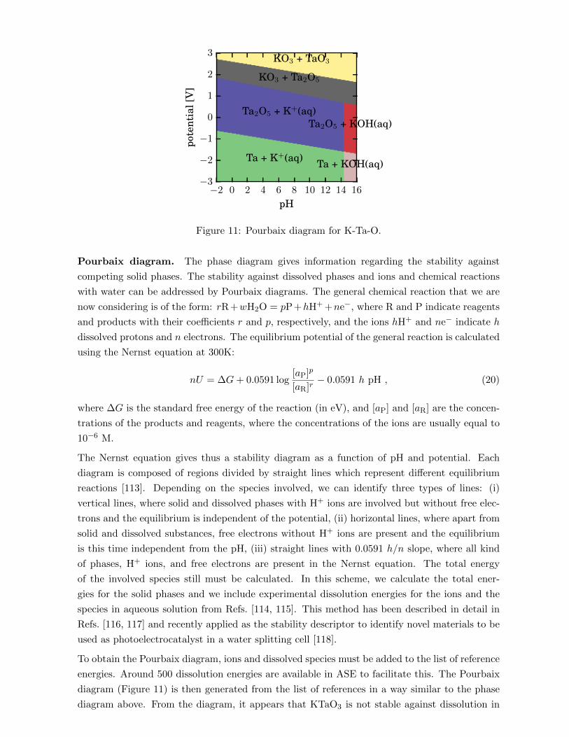
−2 0 2 4 6 8 10 12 14 16

pH

−3

−2

−1

0

1

2

3

pote

ntia

l[V

]

Ta + K+(aq) Ta + KOH(aq)

KO3 + TaO3

Ta2O5 + K+(aq)Ta2O5 + KOH(aq)

KO3 + Ta2O5

Figure 11: Pourbaix diagram for K-Ta-O.

Pourbaix diagram. The phase diagram gives information regarding the stability against

competing solid phases. The stability against dissolved phases and ions and chemical reactions

with water can be addressed by Pourbaix diagrams. The general chemical reaction that we are

now considering is of the form: rR+wH2O = pP+hH+ +ne−, where R and P indicate reagents

and products with their coefficients r and p, respectively, and the ions hH+ and ne− indicate h

dissolved protons and n electrons. The equilibrium potential of the general reaction is calculated

using the Nernst equation at 300K:

nU = ∆G+ 0.0591 log[aP]p

[aR]r− 0.0591 h pH , (20)

where ∆G is the standard free energy of the reaction (in eV), and [aP] and [aR] are the concen-

trations of the products and reagents, where the concentrations of the ions are usually equal to

10−6 M.

The Nernst equation gives thus a stability diagram as a function of pH and potential. Each

diagram is composed of regions divided by straight lines which represent different equilibrium

reactions [113]. Depending on the species involved, we can identify three types of lines: (i)

vertical lines, where solid and dissolved phases with H+ ions are involved but without free elec-

trons and the equilibrium is independent of the potential, (ii) horizontal lines, where apart from

solid and dissolved substances, free electrons without H+ ions are present and the equilibrium

is this time independent from the pH, (iii) straight lines with 0.0591 h/n slope, where all kind

of phases, H+ ions, and free electrons are present in the Nernst equation. The total energy

of the involved species still must be calculated. In this scheme, we calculate the total ener-

gies for the solid phases and we include experimental dissolution energies for the ions and the

species in aqueous solution from Refs. [114, 115]. This method has been described in detail in

Refs. [116, 117] and recently applied as the stability descriptor to identify novel materials to be

used as photoelectrocatalyst in a water splitting cell [118].

To obtain the Pourbaix diagram, ions and dissolved species must be added to the list of reference

energies. Around 500 dissolution energies are available in ASE to facilitate this. The Pourbaix

diagram (Figure 11) is then generated from the list of references in a way similar to the phase

diagram above. From the diagram, it appears that KTaO3 is not stable against dissolution in

the considered range of pH and potential.

So far, the chemical potentials of the involved chemicals are kept fixed at values corresponding

to their standard states. Future releases of the module could include the possibility of tuning

the chemical potentials of the elements.

9 Electronic structure

ASE has several tools that support electronic structure calculations and facilitate post processing

of calculations. DFT calculators can define common methods which return various properties

of the Kohn–Sham states, like eigenvalues, occupation numbers, and the Fermi level. These

methods allow for generic calculations of density of states, band gaps, and related quantities

using methods in ase.dft following any DFT calculation. For calculators that can retrieve the

pseudo wavefunction it is also possible to simulate a simple Tersoff–Hamann [119] STM image

with the ase.dft.stm module.

Calculations with periodic systems usually require Brillouin zone sampling and need a set of

k-points on which the Bloch Hamiltonian is diagonalized. The module ase.dft.kpoints

contains functions that return lists of k-points in a format that is compatible with the elec-

tronic structure calculators supported by ASE. For example, one can ask for a Monkhorst–Pack

grid [120] or a set of k-points along a path in reciprocal space specified by a set of high symmetry

points in the Brillouin zone. The module also contains a dictionary of “standard paths” [121]

in the Brillouin zone for the most common crystal structures. These facilitate systematic cal-

culations of band structures. Below is an example of a script that calculates and plots the

Kohn–Sham band structure of bulk Si using ASE’s BandStructure object. The result is

shown in Figure 12.

from ase.build import bulk

from gpaw import GPAW

si = bulk(’Si’, ’diamond ’, a=5.4)

si.calc = GPAW(mode=’pw’, kpts=(4, 4, 4))

si.get_potential_energy ()

si.calc.set(fixdensity=True ,

kpts={’path’: ’WLGXWK ’, ’npoints ’: 100},

symmetry=’off’)

si.get_potential_energy ()

bs = si.calc.band_structure ()

bs.plot(emax =5.0, filename=’bands_Si.pdf’)

9.1 Estimation of exchange–correlation errors

The major approximation within DFT is the exchange–correlation functional. The BEEFEnsemble

class in ASE provides tools for estimating errors due to the choice of exchange-correlation func-

tional. The most efficient method is tightly linked with the BEEF functionals [122–124]. The

W L Γ X W K

-5

0

5

10

eige

nval

ues

[eV

]

Figure 12: Kohn–Sham band structure of bulk Si.

BEEF-vdW functional [123], which we will use to explain and exemplify the method, has the

functional form

Exc =29∑m=0

amEGGA−xm + αcE

LDA−c + (1− αc)EPBE−c + Enl−c, (21)

where EGGA−xm is GGA exchange with the Legendre polynomial of order m used as enhancement

factor. ELDA−c, EPBE−c, and Enl−c are LDA, PBE, and non-local van der Waals correlation, re-

spectively. The exchange sum expansion coefficients am and the correlation weighting parameter

αc are fitted to databases such that the functional performs well for a range of different proper-

ties [123, 125]. In addition to the best set of coefficients, which constitutes the main BEEF-vdW

functional, an ensemble of functionals with perturbed coefficients are constructed in a procedure

inspired by Bayesian statistics, such that the computed ensemble standard deviation for a given

calculation is a good estimate of the uncertainty and thus also the potential errors for a range

of different properties like reaction enthalpies [123]. The energy of the individual terms in (21)

can be parsed from any interfacing calculator to ASE, which contains the ensemble coefficient

matrices and generates an energy ensemble using simple multiplication operations without any

calls back to the calculator. It is currently implemented for the GPAW and VASP calculators.

As an example, consider two possible reactions in the industrial Fischer–Tropsch process.

CO + 3 H2 → CH4 + H2O (Reaction 1)

CO + 52 H2 → 1

2 C2H6 + H2O (Reaction 2)

The enthalpies of the reactions are calculated and the errors estimated using the ensemble.

In addition, the net reaction difference between the two is simultaneously considered as an

independent reaction.

CH4 → 12 C2H6 + 1

2 H2 (Reaction 3)

Upon comparison with experimental data, see Table 2 and Figure 13, it is found that the errors

versus experimental data and the calculated error estimates are of similar size. Errors and

uncertainties within DFT are often systematic, making relative errors much smaller. Considering

Reaction 3, both the error and the error estimate are one order of magnitude smaller than for

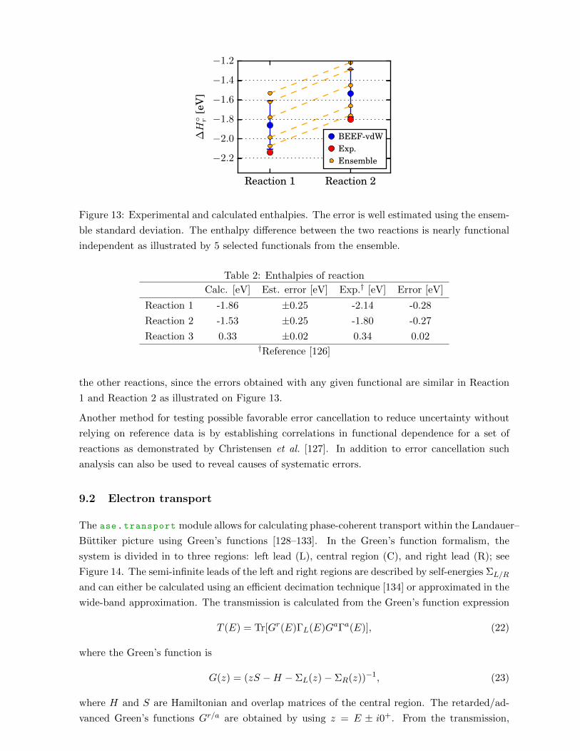
Reaction 1 Reaction 2

−2.2

−2.0

−1.8

−1.6

−1.4

−1.2

∆H◦ r

[eV

]

BEEF-vdWExp.Ensemble

Figure 13: Experimental and calculated enthalpies. The error is well estimated using the ensem-

ble standard deviation. The enthalpy difference between the two reactions is nearly functional

independent as illustrated by 5 selected functionals from the ensemble.

Table 2: Enthalpies of reaction

Calc. [eV] Est. error [eV] Exp.† [eV] Error [eV]

Reaction 1 -1.86 ±0.25 -2.14 -0.28

Reaction 2 -1.53 ±0.25 -1.80 -0.27

Reaction 3 0.33 ±0.02 0.34 0.02†Reference [126]

the other reactions, since the errors obtained with any given functional are similar in Reaction

1 and Reaction 2 as illustrated on Figure 13.

Another method for testing possible favorable error cancellation to reduce uncertainty without

relying on reference data is by establishing correlations in functional dependence for a set of

reactions as demonstrated by Christensen et al. [127]. In addition to error cancellation such

analysis can also be used to reveal causes of systematic errors.

9.2 Electron transport

The ase.transport module allows for calculating phase-coherent transport within the Landauer–

Buttiker picture using Green’s functions [128–133]. In the Green’s function formalism, the

system is divided in to three regions: left lead (L), central region (C), and right lead (R); see

Figure 14. The semi-infinite leads of the left and right regions are described by self-energies ΣL/R

and can either be calculated using an efficient decimation technique [134] or approximated in the

wide-band approximation. The transmission is calculated from the Green’s function expression

T (E) = Tr[Gr(E)ΓL(E)GaΓa(E)], (22)

where the Green’s function is

G(z) = (zS −H − ΣL(z)− ΣR(z))−1, (23)

where H and S are Hamiltonian and overlap matrices of the central region. The retarded/ad-

vanced Green’s functions Gr/a are obtained by using z = E ± i0+. From the transmission,

h h2h1

Central regionPL PL PL PL

Figure 14: Schematic illustration of the transport setup and the matrices h1, h and h2 defining

the left lead, central region and right lead, respectively.

the zero-bias conductance is obtained from the expression G = 2e2

h T (EF ), where e, h and EF

are electronic charge, Planck’s constant and the Fermi energy, respectively. The effect of a

semi-infinite lead α on the central region is described by the self-energy

Σα(E) = (zSCα −HCα)g0α(z)(zS†Cα −H†Cα), (24)

where g0α(z) is a surface Green’s function that is calculated using a decimation technique [134].

The spectral broadening matrices in (22) are given by Γα = i(Σrα − Σa

α).

In the transport module, the C, L and R regions (Figure 14) are specified by three Hamiltonian

matrices h, h1 and h2 (in case of non-orthogonal basis the three overlap matrices s, s1 and s2

are also needed). h1 and h2 should contain two principal layers; a principal layer (PL) being

a periodic part of the Hamiltonian such that there is only coupling between nearest-neighbour

principal layers. By default, the transport module assumes that the coupling between the central

region and lead α, hCα, is the same as the coupling between principal layers. In this case, h

should contain at least one principal layer of lead 1 in its upper left corner, and at least one

principal layer of lead 2 in the lower right corner. See Figure 14.

With the transport module, a number of standard transport properties can be calulated, such

as:

• transmission function

• eigenchannel-resolved transmission functions

• eigenchannel wavefunctions

• projected density of states

and there are various tools for analysis of the transport mechanism:

• rotation to eigenbasis of a subspace, e.g. basis functions on the molecule

• cutting out a subspace, e.g. to see which molecular states are involved in the transport

To illustrate how to use the transport module we consider a simple example consisting of a

junction between graphene leads with zig-zag edges and a benzene molecule linked via alkyne

groups; see Figure 15a. For simplicity we describe the π-system only using a Huckel model

Hamiltonian with all nearest-neighbour hopping elements set to −3 eV and on-site energies set

to zero, i.e. bond length alternation is not taken into account. In this model, the principal layers

hh1

Left Central Right

h2

a)

−2 −1 0 1 2E − EF (eV)

10−6

10−5

10−4

10−3

10−2

10−1

100

Tra

nsm

issi

on

JunctionPristineJunction

b)

c)

d)

e)

Figure 15: a) Structure of the junction. b) Transmission of pristine graphene and of the molecular

junction calculated using Huckel theory. The transmission from a DFT calculation is also shown

for comparison. The vertical lines indicate the molecular states obtained by subdiagonalizing the

molecular subspace. c), d) and e) Left eigenchannel scattering state at an energy corresponding

to the molecular HOMO level, LUMO level and -0.2 eV, respectively. For c) and d) it is for the

Γ k-point, while it is for k = 0.26 A−1

in e).

can be chosen as illustrated in Figure 15a and contain 20 carbon atoms. Periodic boundary

conditions are used in the plane perpendicular to the transport direction and the 1D Brillouin

zone is sampled using 201 k-points. A transport calculation may look like:

calc = TransportCalculator(h=h, h1=h1 , h2=h2 , energies=energies)

transm = calc.get_transmission ()

plt.plot(energies , transm)

In the first line, the transport calculator is set up from the Hamiltonians and a list of energies

for the transmission calculation. Finally, the transmission curve is plotted using matplotlib.

Figure 15b shows the transmission for the junction in the pristine graphene system obtained

using the Huckel model. The pristine graphene system uses the same supercell size perpendicular

to the transport direction. Additionally, the transmission obtained by taking the Hamiltonian

and overlap matrices from a GPAW DFT calculation using a single-zeta local atomic orbital

basis [22, 135] set is shown (Junction∗). We note that the Huckel and DFT results are in good

agreement. The main difference is that the particle–hole transmission symmetry in the Huckel

model caused by the system being an alternant hydrocarbon is broken slightly in the DFT

calculation.

The transmission of the pristine graphene system goes to zero at the Fermi level since the density

of states goes to zero here; graphene can be viewed as zero-bandgap semiconductor. When

considering the transmission of the molecular junction, it is expected to always be below the

pristine system. Interestingly, the transmission at around ±0.2 eV has a peak which approaches

the transmission of the pristine system. This indicates that the charge carriers are not scattered

at all at these energies.

To understand the origin of the broad transmission peaks around ±1.6 eV, indicated by the

black vertical lines, we can use the analysis functions provided by the transport calculator. we

have diagonalized the subspace of the molecule including linkers. This yields the eigenenergies

of the subsystem, and from this we find that the transmission peak position coincides with the

HOMO and LUMO energy.

To further investigate the origin of the transmission peaks we can calculate the eigenchannel

scattering functions.The eigenchannels are calculated using the method of Ref. [136]. Figures 15c

and d visualize the eigenchannel states using coloured circles on the atomic sites; the size of the

circle indicates the absolute weight and the color indicates the phase.

When considering the eigenchannel calculated at the HOMO and LUMO energy found above,

see Figures 15c and d, it resembles the isolated molecule HOMO and LUMO (not shown) to

a large extent. This indicates resonance transmission through the HOMO and LUMO. The

eigenchannel state in Figure 15e has considerable weight on the edges of the graphene leads,

which indicates a transport mechanism involving edge states. It is well known that graphene

zigzag edges have localized edge states at the Dirac point [137].

10 Miscellaneous

10.1 Command-line tools

In addition to the Python library that can be used in Python scripts and programs, an ASE

installation will also include four command-line tools for work on the command line:

• ase-gui: Graphical user interface

• ase-db: Manipulate ASE-databases

• ase-build: Build molecules or crystals

• ase-run: Run simple calculation

The GUI can be used to visualize, manipulate and analyze trajectories. Among the analysis

tools are the possiblity to create x–y plots from the structure and energetics.

The ase-db command-line tool is for querying and manipulating databases as described in detail

in Section 4.1.

Here is an example showing how to use the ase-build and ase-run tools to optimize the

structure of the H2 molucule with the PBE functional:

$ ase -build H2 | ase -run nwchem -p xc=PBE -f 0.02

Running: H2

LBFGS: 0 15:04:19 -31.487747 0.6220

LBFGS: 1 15:04:19 -31.492828 0.0378

LBFGS: 2 15:04:19 -31.492848 0.0020

The ase-build and ase-run tools are very useful for doing quick test calculations, but to get

the most use out of ASE you will need to write scripts that can take advantage of the flexibility

of the Python language.

10.2 Projects using ASE

A number of the calculators listed in Table 1 are developed externally to ASE. For examples,

Atomistica [138] is a library of classical and tight-binding interatomic potentials that can be

compiled as a Python extension module and directly interfaced with ASE. It provides imple-

mentations of empirical bond-order potentials (Abell–Tersoff–Brenner [139–141], REBO2 [142],

etc.), their screened counterparts [143, 144], and embedded atom method potentials [145]. The

non-orthogonal tight-binding module supports charge-selfconsistency [146] and can read a va-

riety of parameter databases. The quippy package is also fully interoperable with ASE. It

provides a calculator for the interatomic potentials implemented in the QUIP Fortran code [45]

such as the Gaussian Approximation Potential [147] as well as support for multiscale QM/MM

calculations [148].

The matscipy package [149], developed by Lars Pastewka and James Kermode, builds on top of

ASE and adds a number of additional general purpose tools for computational materials science,

including a fast neighbour list implemented in C, tools for structure analysis, post processing

and visualisation, a calculator capable of communicating with remote codes over POSIX sockets,

as well as a number of specialist modules targeting specific applications including fracture and

contact mechanics.

10.3 Technical information

ASE is free software licensed under GNU LGPLv2.1 or newer. The source code and documen-

tation are available from the ASE web page https://wiki.fysik.dtu.dk/ase.

ASE requires Python 2 or 3 and the NumPy package. SciPy [19] and MatPlotLib [20] is recom-

mended. The graphical user interface requires PyGTK [150].

Install ASE by running pip install ase (or pip3 install ase for Python 3 users) or see

the web page for alternative methods. The ase-users mailing list or #ase IRC channel on

Freenode.net [151] are available for support.

Everybody is invited to participate in using and developing the code. Coordination and dis-

cussions take place on the mailing list whereas the development takes place on GitLab, at

https://gitlab.com/ase/ase. Please send us bug-reports, patches, code, and ideas.

11 Conclusions

The Atomic Simulation Environment is currently in use by many researchers working on diverse

applications within condensed matter physics, chemistry, and other fields. There are also quite

a few developers adding new features to the environment. So what can be expected from ASE

in the future?

At the present stage the core structure of ASE dealing with the basic properties of atoms

and calculators is well developed, and it is therefore straightforward to add new functionality.

For example, new interfaces to the ONETEP [152] and Amber [153] codes are currently being

implemented. In the near future we hope to see further development in several areas. To mention

some of them: 1) New screening or search methods (like the currently implemented genetic

algorithm) using machine learning could be implemented. 2) The analysis of the electronic

information obtained by DFT calculations could be significantly improved. Recently a way

of calculating band structures was introduced but there is a general need for more detailed

analysis based on electronic spectra, densities, or wave functions. 3) Crystal symmetry analysis is

currently done mostly by the DFT codes. This task could be done directly by ASE. 4) Currently

some of the external codes like CP2K and GPAW are “kept alive” when atoms are moved to

avoid computational overhead when restarting a calculation. This could be implemented in a

more generic way in ASE so that other calculators easily could obtain this feature. 5) The fairly

new database module allows for storage and retrieval of DFT calculations. The database can

be used to keep track of the status of many similar calculations performed for example in a

computational screening study. However, there are currently no utility functions or classes to

perform this task in an easy way.

The users of ASE benefit from the large number of functions available for setting up, controlling,

and analyzing simulations based on many different calculators, and from the large flexibility

in the Python language itself to construct loops and to allow for interplay between different

simulations. As the number of available calculators increases and new functionality is added,

ASE will hopefully become an even more attractive toolbox contributing to efficient development

and utilization of electronic structure theory and molecular dynamics simulations. We hope that

ASE will also encourage and contribute to further collaborative efforts with open exchange of

not only data and results but also efficient scripting to the benefit of the research community.

12 Acknowledgements

The authors acknowledge funding from: The European Union’s Horizon 2020 research and

innovation program under grant agreement no. 676580 with The Novel Materials Discovery

(NOMAD) Laboratory, a European Center of Excellence; research grant 9455 from VILLUM

FONDEN; Deutsche Forschungsgemeinschaft (grant PA2023/2); the UK Engineering and Phys-

ical Sciences Research Council (grants EP/L014742/1, EP/L027682/1 and EP/P002188/1).

References

[1] R.O. Jones. Density functional theory: Its origins, rise to prominence, and future. Reviews

of Modern Physics, 87(3):897–923, August 2015.

[2] Quantum chemistry and solid-state physics software. https://en.wikipedia.org/wiki/

List_of_quantum_chemistry_and_solid-state_physics_software.

[3] Knowledgebase of interatomic models. https://openkim.org.

[4] Paul F. Dubois. Making Applications Programmable. Computers in Physics, 8(1):70–73,

January 1994.

[5] Erich Gamma, Richard Helm, Ralph Johnson, and John Vlissides. Design Patterns. Ele-

ments of Reusable Object-Oriented Software. Addison-Wesley, 1995.

[6] Sune R. Bahn and Karsten W. Jacobsen. An object-oriented scripting interface to a legacy

electronic structure code. Computing in Science & Engineering, 4(3):56–66, 2002.

[7] DACAPO code. https://wiki.fysik.dtu.dk/dacapo.

[8] NumPy. http://www.numpy.org.

[9] Greg Mills and Hannes Jonsson. Quantum and thermal effects in H2 dissociative adsorp-

tion: Evaluation of free energy barriers in multidimensional quantum systems. Physical

Review Letters, 72(7):1124–1127, February 1994.

[10] Hannes Jonsson, Greg Mills, and Karsten Wedel Jacobsen. Nudged elastic band method

for finding minimum energy paths of transitions. In Bruce J. Berne, Giovanni Ciccotti,

and David F. Coker, editors, Classical and Quantum Dynamics in Condensed Phased

Simulations, Proceedings of the International School of Physics “Computer Simulation

of Rare Events and Dynamics of Classical and Quantum Condensed-Phased Systems” :

Lerici, Villa Marigola, 7 July-18 July 1997, pages 385–404. World Scientific Publishing

Company Incorporated, January 1998.

[11] Alireza Khorshidi and Andrew A. Peterson. Amp: A modular approach to machine learn-

ing in atomistic simulations. Comput. Phys. Commun., 207:310–324, 2016.

[12] Travis E. Oliphant. Python for scientific computing. Computing in Science & Engineering,

9(3):10–20, 2007.

[13] K. Jarrod Millman and Michael Aivazis. Python for scientists and engineers. Computing

in Science & Engineering, 13(2):9–12, 2011.

[14] Stefan van der Walt, S. Chris Colbert, and Gael Varoquaux. The numpy array: A structure

for efficient numerical computation. Computing in Science & Engineering, 13(2):22–30,

2011.

[15] Ricky A. Kendall, Edoardo Apra, David E. Bernholdt, Eric J. Bylaska, Michel Dupuis,

George I. Fann, Robert J. Harrison, Jialin Ju, Jeffrey A. Nichols, Jarek Nieplocha, T.P.

Straatsma, Theresa L. Windus, and Adrian T. Wong. High performance computational

chemistry: An overview of NWChem a distributed parallel application. Comput. Phys.

Commun., 128(1-2):260–283, jun 2000.

[16] M. Valiev, E.J. Bylaska, N. Govind, K. Kowalski, T.P. Straatsma, H.J.J. Van Dam,

D. Wang, J. Nieplocha, E. Apra, T.L. Windus, and W.A. de Jong. NWChem: A compre-

hensive and scalable open-source solution for large scale molecular simulations. Comput.

Phys. Commun., 181(9):1477–1489, sep 2010.

[17] John P. Perdew, Kieron Burke, and Matthias Ernzerhof. Generalized Gradient Approxi-

mation Made Simple. Phys. Rev. Lett., 77(18):3865–3868, 1996.

[18] Jorge Nocedal and Steve J. Wright. Numerical optimization. Springer Series in Operations

Research and Financial Engineering. Springer, Berlin, 2006.

[19] SciPy. http://scipy.org.

[20] matplotlib. http://matplotlib.org/.

[21] J. J. Mortensen, L. B. Hansen, and K. W. Jacobsen. Real-space grid implementation of

the projector augmented wave method. Phys. Rev. B, 71:035109, Jan 2005.

[22] J. Enkovaara, C. Rostgaard, J. J. Mortensen, J. Chen, M. Du lak, L. Ferrighi, J. Gavnholt,

C. Glinsvad, V. Haikola, H. A. Hansen, H. H. Kristoffersen, M. Kuisma, A. H. Larsen,

L. Lehtovaara, M. Ljungberg, O. Lopez-Acevedo, P. G. Moses, J. Ojanen, T. Olsen, V. Pet-

zold, N. A. Romero, J. Stausholm-Møller, M. Strange, G. A. Tritsaris, M. Vanin, M. Wal-

ter, B. Hammer, H. Hakkinen, G. K. H. Madsen, R. M. Nieminen, J. K. Nørskov, M. Puska,

T. T. Rantala, J. Schiøtz, K. S. Thygesen, and K. W. Jacobsen. Electronic structure calcu-

lations with GPAW: a real-space implementation of the projector augmented-wave method.

Journal of Physics: Condensed Matter, 22(25):253202, 2010.

[23] X. Gonze, B. Amadon, P.-M. Anglade, J.-M. Beuken, F. Bottin, P. Boulanger, F. Bruneval,

D. Caliste, R. Caracas, M. Cote, T. Deutsch, L. Genovese, Ph. Ghosez, M. Giantomassi,

S. Goedecker, D.R. Hamann, P. Hermet, F. Jollet, G. Jomard, S. Leroux, M. Mancini,

S. Mazevet, M.J.T. Oliveira, G. Onida, Y. Pouillon, T. Rangel, G.-M. Rignanese, D. San-

galli, R. Shaltaf, M. Torrent, M.J. Verstraete, G. Zerah, and J.W. Zwanziger. ABINIT:

First-principles approach to material and nanosystem properties. Computer Physics Com-

munications, 180(12):2582 – 2615, 2009.

[24] Stewart J. Clark, Matthew D. Segall, Chris J. Pickard, Phil J. Hasnip, Matt I.J. Probert,

Keith Refson, and Mike C. Payne. First principles methods using CASTEP. Zeitschrift

fur Kristallographie-Crystalline Materials, 220(5/6):567–570, 2005.

[25] Jurg Hutter, Marcella Iannuzzi, Florian Schiffmann, and Joost VandeVondele. CP2K:

atomistic simulations of condensed matter systems. Wiley Interdisciplinary Reviews: Com-

putational Molecular Science, 4(1):15–25, 2014.

[26] Andreas M. Koster, Patrizia Calaminici, Mark E. Casida, Roberto Flores-Moreno, Gerald

Geudtner, Annick Goursot, Thomas Heine, Andrei Ipatov, Florian Janetzko, Jorge M. del

Campo, Serguei Patchkovskii, J. Ulises Reveles, Dennis R. Salahub, Alberto Vela, and

deMon developers. deMon2k, 2006.

[27] B. Aradi, B. Hourahine, and Th. Frauenheim. DFTB+, a sparse matrix-based implemen-

tation of the DFTB method. The Journal of Physical Chemistry A, 111(26):5678–5684,

2007. PMID: 17567110.

[28] Murray S. Daw and M. I. Baskes. Semiempirical, quantum mechanical calculation of

hydrogen embrittlement in metals. Phys. Rev. Lett., 50:1285–1288, Apr 1983.

[29] Karsten W. Jacobsen, P. Stoltze, and J. K. Nørskov. A semi-empirical effective medium

theory for metals and alloys. Surf. Sci., 366(2):394–402, 1996.

[30] Andris Gulans, Stefan Kontur, Christian Meisenbichler, Dmitrii Nabok, Pasquale Pavone,

Santiago Rigamonti, Stephan Sagmeister, Ute Werner, and Claudia Draxl. exciting: a

full-potential all-electron package implementing density-functional theory and many-body

perturbation theory. Journal of Physics: Condensed Matter, 26(36):363202, 2014.

[31] Volker Blum, Ralf Gehrke, Felix Hanke, Paula Havu, Ville Havu, Xinguo Ren, Karsten

Reuter, and Matthias Scheffler. Ab initio molecular simulations with numeric atom-

centered orbitals. Computer Physics Communications, 180(11):2175 – 2196, 2009.

[32] E. Wimmer, H. Krakauer, M. Weinert, and A. J. Freeman. Full-potential self-

consistent linearized-augmented-plane-wave method for calculating the electronic struc-

ture of molecules and surfaces: O2 molecule. Phys. Rev. B, 24:864–875, Jul 1981.

[33] M. J. Frisch, G. W. Trucks, H. B. Schlegel, G. E. Scuseria, M. A. Robb, J. R. Cheeseman,

J. A. Montgomery, Jr., T. Vreven, K. N. Kudin, J. C. Burant, J. M. Millam, S. S. Iyengar,

J. Tomasi, V. Barone, B. Mennucci, M. Cossi, G. Scalmani, N. Rega, G. A. Petersson,

H. Nakatsuji, M. Hada, M. Ehara, K. Toyota, R. Fukuda, J. Hasegawa, M. Ishida, T. Naka-

jima, Y. Honda, O. Kitao, H. Nakai, M. Klene, X. Li, J. E. Knox, H. P. Hratchian, J. B.

Cross, V. Bakken, C. Adamo, J. Jaramillo, R. Gomperts, R. E. Stratmann, O. Yazyev,

A. J. Austin, R. Cammi, C. Pomelli, J. W. Ochterski, P. Y. Ayala, K. Morokuma, G. A.

Voth, P. Salvador, J. J. Dannenberg, V. G. Zakrzewski, S. Dapprich, A. D. Daniels, M. C.

Strain, O. Farkas, D. K. Malick, A. D. Rabuck, K. Raghavachari, J. B. Foresman, J. V. Or-

tiz, Q. Cui, A. G. Baboul, S. Clifford, J. Cioslowski, B. B. Stefanov, G. Liu, A. Liashenko,

P. Piskorz, I. Komaromi, R. L. Martin, D. J. Fox, T. Keith, M. A. Al-Laham, C. Y. Peng,

A. Nanayakkara, M. Challacombe, P. M. W. Gill, B. Johnson, W. Chen, M. W. Wong,

C. Gonzalez, and J. A. Pople. Gaussian 03, Revision C.02. Gaussian, Inc., Wallingford,

CT, 2004.

[34] Sander Pronk, Szilard Pall, Roland Schulz, Per Larsson, Par Bjelkmar, Rossen Apostolov,

Michael R. Shirts, Jeremy C. Smith, Peter M. Kasson, David van der Spoel, Berk Hess,

and Erik Lindahl. GROMACS 4.5: a high-throughput and highly parallel open source

molecular simulation toolkit. Bioinformatics, 29(7):845–854, 2013.

[35] V. Makinen P. Koskinen. Density-functional tight-binding for beginners. Computational

Material Science, 47:237, 2009.

[36] Sohrab Ismail-Beigi and T.A. Arias. New algebraic formulation of density functional

calculation. Computer Physics Communications, 128(1–2):1 – 45, 2000.

[37] Steve Plimpton. Fast parallel algorithms for short-range molecular dynamics. Journal of

Computational Physics, 117(1):1 – 19, 1995.

[38] J. E. Jones. On the determination of molecular fields. II. from the equation of state of a

gas. Proceedings of the Royal Society of London A: Mathematical, Physical and Engineering

Sciences, 106(738):463–477, 1924.

[39] James J. P. Stewart. MOPAC: A semiempirical molecular orbital program. Journal of

Computer-Aided Molecular Design, 4(1):1–103, 1990.

[40] Philip M. Morse. Diatomic molecules according to the wave mechanics. II. vibrational

levels. Phys. Rev., 34:57–64, Jul 1929.

[41] M. Valiev, E.J. Bylaska, N. Govind, K. Kowalski, T.P. Straatsma, H.J.J. Van Dam,

D. Wang, J. Nieplocha, E. Apra, T.L. Windus, and W.A. de Jong. NWChem: A compre-

hensive and scalable open-source solution for large scale molecular simulations. Computer

Physics Communications, 181(9):1477 – 1489, 2010.

[42] Xavier Andrade, David Strubbe, Umberto De Giovannini, Ask Hjorth Larsen, Micael

J. T. Oliveira, Joseba Alberdi-Rodriguez, Alejandro Varas, Iris Theophilou, Nicole Helbig,

Matthieu J. Verstraete, Lorenzo Stella, Fernando Nogueira, Alan Aspuru-Guzik, Alberto

Castro, Miguel A. L. Marques, and Angel Rubio. Real-space grids and the Octopus code

as tools for the development of new simulation approaches for electronic systems. Phys.

Chem. Chem. Phys., 17:31371–31396, 2015.

[43] E. B. Tadmor, R. S. Elliott, J. P. Sethna, R. E. Miller, and C. A. Becker. The potential of

atomistic simulations and the knowledgebase of interatomic models. JOM, 63(7):17, 2011.

[44] Paolo Giannozzi, Stefano Baroni, Nicola Bonini, Matteo Calandra, Roberto Car, Carlo

Cavazzoni, Davide Ceresoli, Guido L. Chiarotti, Matteo Cococcioni, Ismaila Dabo, Andrea

Dal Corso, Stefano de Gironcoli, Stefano Fabris, Guido Fratesi, Ralph Gebauer, Uwe Ger-

stmann, Christos Gougoussis, Anton Kokalj, Michele Lazzeri, Layla Martin-Samos, Nicola

Marzari, Francesco Mauri, Riccardo Mazzarello, Stefano Paolini, Alfredo Pasquarello,

Lorenzo Paulatto, Carlo Sbraccia, Sandro Scandolo, Gabriele Sclauzero, Ari P. Seitso-

nen, Alexander Smogunov, Paolo Umari, and Renata M. Wentzcovitch. QUANTUM

ESPRESSO: a modular and open-source software project for quantum simulations of ma-

terials. Journal of Physics: Condensed Matter, 21(39):395502 (19pp), 2009.

[45] Gabor Csanyi, Steven Winfield, James R. Kermode, Alessandro de Vita, Alessio Comisso,

Noam Bernstein, and Mike C. Payne. Expressive Programming for Computational Physics

in Fortran 95. IoP Comput Phys Newsl., page Spring 2007, 2007.

[46] Jose M. Soler, Emilio Artacho, Julian D. Gale, Alberto Garcıa, Javier Junquera, Pablo

Ordejon, and Daniel Sanchez-Portal. The SIESTA method for ab initio order-N materials

simulation. Journal of Physics: Condensed Matter, 14(11):2745, 2002.

[47] William L. Jorgensen, Jayaraman Chandrasekhar, Jeffry D. Madura, Roger W. Impey, and

Michael L. Klein. Comparison of simple potential functions for simulating liquid water.

The Journal of Chemical Physics, 79(2):926–935, 1983.

[48] Filipp Furche, Reinhart Ahlrichs, Christof Hattig, Wim Klopper, Marek Sierka, and Flo-

rian Weigend. Turbomole. Wiley Interdisciplinary Reviews: Computational Molecular

Science, 4(2):91–100, 2014.

[49] G. Kresse and J. Furthmuller. Efficient iterative schemes for ab initio total-energy calcu-

lations using a plane-wave basis set. Phys. Rev. B, 54:11169–11186, Oct 1996.

[50] Alexandre Tkatchenko and Matthias Scheffler. Accurate molecular van der Waals interac-

tions from ground-state electron density and free-atom reference data. Phys. Rev. Lett.,

102:073005, Feb 2009.

[51] Stefan Grimme, Jens Antony, Stephan Ehrlich, and Helge Krieg. A consistent and accurate

ab initio parametrization of density functional dispersion correction (DFT-D) for the 94

elements H–Pu. The Journal of Chemical Physics, 132(15), 2010.

[52] Stefan Grimme, Stephan Ehrlich, and Lars Goerigk. Effect of the damping function

in dispersion corrected density functional theory. Journal of Computational Chemistry,

32(7):1456–1465, 2011.

[53] Grimme D3 ASE calculator. https://gitlab.com/ehermes/ased3.

[54] Robin Haunschild and Wim Klopper. New accurate reference energies for the G2/97 test

set. The Journal of Chemical Physics, 136(16), 2012.

[55] T. Hahn. International Tables for Crystallography, Space-Group Symmetry. International

Tables for Crystallography. Wiley, 2005.

[56] C. Emil Tripa, Tykhon S. Zubkov, John T. Yates, Manos Mavrikakis, and Jens K. Nørskov.

Molecular N2 chemisorption—specific adsorption on step defect sites on Pt surfaces. The

Journal of Chemical Physics, 111(18):8651–8658, 1999.

[57] Hans-Joachim Freund and Gianfranco Pacchioni. Oxide ultra-thin films on metals: new

materials for the design of supported metal catalysts. Chemical Society Reviews, 37:2224–

2242, 2008.

[58] Shuifen Xie, Sang-il Choi, Ning Lu, Luke Roling, Jeffrey Herron, Lei Zhang, Jinguo Wang,

Moon Kim, Zhaoxiong Xie, Manos Mavrikakis, and Younan Xia. Atomic layer-by-layer

deposition of Pt on Pd nanocubes for catalysts with enhanced activity and durability

toward oxygen reduction atomic layer-by-layer deposition of Pt on Pd nanocubes for cat-

alysts with enhanced activity and durability toward oxygen. Nano Letters, 14:3570–3576,

2014.

[59] Randall Munroe. xkcd. https://xkcd.com/927/.

[60] POV-Ray. http://www.povray.org/.

[61] Alim B. Alchagirov, John P. Perdew, Jonathan C. Boettger, R. C. Albers, and Carlos

Fiolhais. Reply to “Comment on ‘Energy and pressure versus volume: Equations of state

motivated by the stabilized jellium model’ ”. Phys. Rev. B, 67:026103, Jan 2003.

[62] W.K. Yu, J.S. Wu, and D.K. Panda. Fast and scalable startup of MPI programs in

InfiniBand clusters. In Bouge, L. and Prasanna, V.K., editor, High performance computing

- HIPC 2004, volume 3296 of Lecture notes in computer science, pages 440–449, 2004. 11th

International Conference on High Performance Computing, Bangalore, INDIA, DEC 19-

22, 2004.

[63] CP2K code. https://www.cp2k.org.

[64] Standard for information technology portable operating system interface (POSIX(R)) base

specifications, issue 7. IEEE Std 1003.1, 2013 Edition (incorporates IEEE Std 1003.1-2008,

and IEEE Std 1003.1-2008/Cor 1-2013), pages 1–3906, April 2013.

[65] D. Frenkel and B. Smit. Understanding Molecular Simulation: From Algorithms to Appli-

cations. Academic Press. Academic Press, 2002.

[66] H. J. C. Berendsen, J. P. M. Postma, W. F. van Gunsteren, A. DiNola, and J. R. Haak.

Molecular dynamics with coupling to an external bath. The Journal of chemical physics,

81(8):3684, 1984.

[67] M.P. Allen and D.J. Tildesley. Computer Simulation of Liquids. Oxford Science Publ.

Clarendon Press, 1989.

[68] W. G. Hoover. Canonical Dynamics - Equilibrium Phase-Space Distributions. Phys. Rev.

A, 31(3):1695–1697, 1985.

[69] William G. Hoover. Constant-pressure equations of motion. Phys. Rev. A, 34(3):2499–

2500, September 1986.

[70] M. Parrinello and A. Rahman. Crystal-Structure and Pair Potentials — a Molecular-

Dynamics Study. Phys. Rev. Lett., 45(14):1196–1199, 1980.

[71] M. Parrinello and A. Rahman. Polymorphic Transitions in Single-Crystals — a New

Molecular-Dynamics Method. Journal of Applied Physics, 52(12):7182–7190, 1981.

[72] S. Melchionna. Erratum: Constrained systems and statistical distribution [Phys. Rev. E

61, 6165 (2000)]. Phys. Rev. E, 62(4):5864–5864, 2000.

[73] S. Melchionna. Constrained systems and statistical distribution. Phys. Rev. E, 61(6):6165–

6170, 2000.

[74] W.H. Press, S.A. Teukolsky, W.T. Vetterling, and B.P. Flannery. Numerical Recipes in

C. Cambridge University Press, Cambridge, 1992.

[75] Jorge Nocedal. Updating quasi-Newton matrices with limited storage. Math. Comp.,

35(151):773–782, 1980.

[76] Dong C. Liu and Jorge Nocedal. On the limited memory bfgs method for large scale

optimization. Mathematical Programming, 45(1):503–528, 1989.

[77] Erik Bitzek, Pekka Koskinen, Franz Gahler, Michael Moseler, and Peter Gumbsch. Struc-

tural relaxation made simple. Phys. Rev. Lett., 97:170201, Oct 2006.

[78] David Packwood, James Kermode, Letif Mones, Noam Bernstein, John Woolley, Nicholas

Gould, Christoph Ortner, and Gabor Csanyi. A universal preconditioner for simulating

condensed phase materials. J. Chem. Phys., 144(16):164109, 28 April 2016.

[79] Andrew A. Peterson. Global optimization of adsorbate–surface structures while preserving

molecular identity. Topics in Catalysis, 57(1-4):40–53, 2014.

[80] Graeme Henkelman and Hannes Jonsson. Improved tangent estimate in the nudged elastic

band method for finding minimum energy paths and saddle points. J. Chem. Phys.,

113(22):9978–9985, 2000.

[81] Graeme Henkelman, Blas P. Uberuaga, and Hannes Jonsson. A climbing image nudged

elastic band method for finding saddle points and minimum energy paths. The Journal of

Chemical Physics, 113(22):9901–9904, 2000.

[82] Søren Smidstrup, Andreas Pedersen, Kurt Stokbro, and Hannes Jonsson. Improved initial

guess for minimum energy path calculations. J. Chem. Phys., 140(21), 2014.

[83] E. L. Kolsbjerg, M. M. Groves, and B. Hammer. An automated nudged elastic band

method. The Journal of Chemical Physics, 145(9), 2016.

[84] A. M. H. Rasmussen, M. N. Groves, and B. Hammer. Remote activation of chemical bonds

in heterogeneous catalysis. ACS Cat., 4:1182–1188, 2014.

[85] G. Goubert, A. M. H. Rasmussen, Yi Dong, M. N. Groves, P. H. McBreen, and B. Hammer.

Walking-like diffusion of two-footed asymmetric aromatic adsorbates on Pt(111). Surf.

Sci., 629:123–131, 2014.

[86] E. L. Kolsbjerg, M. N. Groves, and B. Hammer. Pyridine adsorption and diffusion on

Pt(111) investigated with density functional theory. J. Chem. Phys., 144(16), 2016.

[87] Marko Melander, Kari Laasonen, and Hannes Jonsson. Removing external degrees of

freedom from transition-state search methods using quaternions. Journal of Chemical

Theory and Computation, 11(3):1055–1062, 2015.

[88] Andreas Pedersen, Sigurdur F. Hafstein, and Hannes Jonsson. Efficient Sampling of Saddle

Points with the Minimum-Mode Following Method. SIAM Journal on Scientific Comput-

ing, 33(2):633–652, 2011.

[89] David J. Wales and Jonathan P. K. Doye. Global optimization by basin-hopping and the

lowest energy structures of Lennard-Jones clusters containing up to 110 atoms. J. Phys.

Chem. A, 101:5111–5116, 1997.

[90] Stefan Goedecker. Minima hopping: An efficient search method for the global minimum

of the potential energy surface of complex molecular systems. The Journal of Chemical

Physics, 120(21):9911–9917, 2004.

[91] David E. Goldberg. Genetic Algorithms in Search, Optimization, and Machine Learning.

Addison-Wesley Professional, 1989.

[92] S. Forrest. Genetic algorithms: principles of natural selection applied to computation.

Science (New York, N.Y.), 261(5123):872–8, aug 1993.

[93] R.L. Johnston. Evolving better nanoparticles: Genetic algorithms for optimising cluster

geometries. Dalton Trans., pages 4193–4207, 2003.

[94] Colin W. Glass, Artem R. Oganov, and Nikolaus Hansen. USPEX – Evolutionary crystal

structure prediction. Computer Physics Communications, 175(11-12):713–720, dec 2006.

[95] G. Johannesson, T. Bligaard, A. Ruban, H. Skriver, K. Jacobsen, and J. Nørskov. Com-

bined Electronic Structure and Evolutionary Search Approach to Materials Design. Phys-

ical Review Letters, 88(25):1–5, jun 2002.

[96] Steen Lysgaard, David D. Landis, Thomas Bligaard, and Tejs Vegge. Genetic Algorithm

Procreation Operators for Alloy Nanoparticle Catalysts. Topics in Catalysis, 57(1–4):33–

39, 2014.

[97] Steen Lysgaard, Jon S. G. Myrdal, Heine A. Hansen, and Tejs Vegge. A DFT-based

genetic algorithm search for AuCu nanoalloy electrocatalysts for CO2 reduction. Physical

chemistry chemical physics : PCCP, 17(42):28270–6, nov 2015.

[98] Lasse Vilhelmsen and Bjørk Hammer. Systematic Study of Au6 to Au12 Gold Clus-

ters on MgO(100) F Centers Using Density-Functional Theory. Physical Review Letters,

108(12):126101, mar 2012.

[99] D. M. Deaven and K. M. Ho. Molecular-Geometry Optimization With A Genetic Algo-

rithm. Physical Review Letters, 75(2):288–291, jul 1995.

[100] Lasse B. Vilhelmsen and Bjørk Hammer. A genetic algorithm for first principles global

structure optimization of supported nano structures. The Journal of chemical physics,

141(4):044711, jul 2014.

[101] Peter Bjerre Jensen, Steen Lysgaard, Ulrich J. Quaade, and Tejs Vegge. Designing Mixed

Metal Halide Ammines for Ammonia Storage Using Density Functional Theory and Ge-

netic Algorithms. Physical Chemistry Chemical Physics, 16(36):19732–19740, aug 2014.

[102] Peter B. Jensen, Agata Bialy, Didier Blanchard, Steen Lysgaard, Alexander K. Reumert,

Ulrich J. Quaade, and Tejs Vegge. Accelerated DFT-Based Design of Materials for Am-

monia Storage. Chemistry of Materials, 27(13):4552–4561, jul 2015.

[103] Thomas Frederiksen, Magnus Paulsson, Mads Brandbyge, and Antti-Pekka Jauho. In-

elastic transport theory from first-principles: methodology and applications for nanoscale

devices. Phys. Rev. B, 75:205413, 2007.

[104] Dirk Porezag and Mark R. Pederson. Infrared intensities and raman-scattering activities

within density-functional theory. Phys. Rev. B, 54:7830–7836, Sep 1996.

[105] Mickael Profeta and Francesco Mauri. Theory of resonant raman scattering of tetrahedral

amorphous carbon. Phys. Rev. B, 63:245415, 2001.

[106] M.T. Dove. Introduction to Lattice Dynamics. Cambridge Topics in Mineral Physics and

Chemistry. Cambridge University Press, 1993.

[107] Dario Alfe. PHON: A program to calculate phonons using the small displacement method.

Comput. Phys. Commun., 180(12):2622–2633, 2009.

[108] Stefano Baroni, Paolo Giannozzi, and Andrea Testa. Green’s-Function Approach to Linear

Response in Solids. Phys. Rev. Lett., 58(18), 1987.

[109] Glenn Jones, Jon Geest Jakobsen, Signe S. Shim, Jesper Kleis, Martin P. Andersson,

Jan Rossmeisl, Frank Abild-Pedersen, Thomas Bligaard, Stig Helveg, Berit Hinnemann,

Jens R. Rostrup-Nielsen, Ib Chorkendorff, Jens Sehested, and Jens K. Nørskov. First prin-

ciples calculations and experimental insight into methane steam reforming over transition

metal catalysts. Journal of Catalysis, 259(1):147–160, 2008.

[110] Terrell L. Hill. An Introduction to Statistical Thermodynamics. Addison–Wesley Publish-

ing Company, Inc., 1960.

[111] Christopher J. Cramer. Essentials of Computational Chemistry. Wiley, 2nd edition, 2004.

[112] Donald Allan McQuarrie. Statistical Mechanics. University Science Books, 2000.

[113] E. D. Verink. Simplified Procedure for Constructing Pourbaix Diagrams. Wiley, 2011.

[114] James W. Johnson, Eric H. Oelkers, and Harold C. Helgeson. SUPCRT92: A software

package for calculating the standard molal thermodynamic properties of minerals, gases,

aqueous species, and reactions from 1 to 5000 bar and 0 to 1000◦C. Computers & Geo-

sciences, 18(7):899 – 947, 1992.

[115] Marcel Pourbaix. Atlas of electrochemical equilibria in aqueous solutions. Pergamon Press,

1st edition, 1966.

[116] Kristin A. Persson, Bryn Waldwick, Predrag Lazic, and Gerbrand Ceder. Prediction of

solid–aqueous equilibria: Scheme to combine first-principles calculations of solids with

experimental aqueous states. Phys. Rev. B, 85:235438, Jun 2012.

[117] Ivano E. Castelli, Kristian S. Thygesen, and Karsten W. Jacobsen. Calculated pourbaix

diagrams of cubic perovskites for water splitting: Stability against corrosion. Topics in

Catalysis, 57(1):265–272, 2013.

[118] Ivano E. Castelli, Falco Huser, Mohnish Pandey, Hong Li, Kristian S. Thygesen, Brian

Seger, Anubhav Jain, Kristin A. Persson, Gerbrand Ceder, and Karsten W. Jacobsen.

New light-harvesting materials using accurate and efficient bandgap calculations. Advanced

Energy Materials, 5(2):1400915, 2015.

[119] J. Tersoff and D. R. Hamann. Theory of the scanning tunneling microscope. Phys. Rev.

B, 31:805–813, Jan 1985.

[120] Hendrik J. Monkhorst and James D. Pack. Special points for Brillouin-zone integrations.

Phys. Rev. B, 13(12):5188–5192, 1976.

[121] Wahyu Setyawan and Stefano Curtarolo. High-throughput electronic band structure cal-

culations: challenges and tools. Computational Materials Science, 49:299–312, 2010.

[122] J. J. Mortensen, K. Kaasbjerg, S. L. Frederiksen, J. K. Nørskov, J. P. Sethna, and

K. W. Jacobsen. Bayesian error estimation in density-functional theory. Phys. Rev. Lett.,

95:216401, Nov 2005.

[123] Jess Wellendorff, Keld T. Lundgaard, Andreas Møgelhøj, Vivien Petzold, David D. Landis,

Jens K. Nørskov, Thomas Bligaard, and Karsten W. Jacobsen. Density functionals for

surface science: Exchange–correlation model development with Bayesian error estimation.

Phys. Rev. B, 85:235149, Jun 2012.

[124] Jess Wellendorff, Keld T. Lundgaard, Karsten W. Jacobsen, and Thomas Bligaard.

mBEEF: An accurate semi-local Bayesian error estimation density functional. The Journal

of Chemical Physics, 140(14), 2014.

[125] Jess Wellendorff, Trent L. Silbaugh, Delfina Garcia-Pintos, Jens K. Nørskov, Thomas

Bligaard, Felix Studt, and Charles T. Campbell. A benchmark database for adsorption

bond energies to transition metal surfaces and comparison to selected DFT functionals.

Surface Science, 640:36 – 44, 2015. Reactivity Concepts at Surfaces: Coupling Theory

with Experiment.

[126] P. J. Linstrom and W. G. Mallard, editors. NIST Chemistry WebBook, NIST Standard

Reference Database Number 69. National Institute of Standards and Technology, June

2005.

[127] Rune Christensen, Heine A. Hansen, and Tejs Vegge. Identifying systematic DFT errors

in catalytic reactions. Catal. Sci. Technol., 5:4946–4949, 2015.

[128] R. Landauer. Spatial variation of currents and fields due to localized scatterers in metallic

conduction. IBM Journal of Research and Development, 1(3):223–231, July 1957.

[129] Rolf Landauer. Electrical resistance of disordered one-dimensional lattices. Philosophical

Magazine, 21(172):863–867, 1970.

[130] C. Caroli, R. Combescot, P. Nozieres, and D. Saint-James. Direct calculation of the

tunneling current. Journal of Physics C: Solid State Physics, 4(8):916, 1971.

[131] Yigal Meir and Ned S. Wingreen. Landauer formula for the current through an interacting

electron region. Phys. Rev. Lett., 68:2512–2515, Apr 1992.

[132] Mads Brandbyge, Jose-Luis Mozos, Pablo Ordejon, Jeremy Taylor, and Kurt Stokbro.

Density-functional method for nonequilibrium electron transport. Phys. Rev. B, 65:165401,

Mar 2002.

[133] M. Strange, I. S. Kristensen, K. S. Thygesen, and K. W. Jacobsen. Benchmark den-

sity functional theory calculations for nanoscale conductance. The Journal of Chemical

Physics, 128(11), 2008.

[134] F. Guinea, C. Tejedor, F. Flores, and E. Louis. Effective two-dimensional Hamiltonian at

surfaces. Phys. Rev. B, 28:4397–4402, Oct 1983.

[135] A. H. Larsen, M. Vanin, J. J. Mortensen, K. S. Thygesen, and K. W. Jacobsen. Localized

atomic basis set in the projector augmented wave method. Phys. Rev. B, 80:195112, Nov

2009.

[136] Magnus Paulsson and Mads Brandbyge. Transmission eigenchannels from nonequilibrium

Green’s functions. Phys. Rev. B, 76:115117, Sep 2007.

[137] Kyoko Nakada, Mitsutaka Fujita, Gene Dresselhaus, and Mildred S. Dresselhaus. Edge

state in graphene ribbons: Nanometer size effect and edge shape dependence. Phys. Rev.

B, 54:17954–17961, Dec 1996.

[138] Atomistica. https://github.com/Atomistica/atomistica.

[139] G. C. Abell. Empirical chemical pseudopotential theory of molecular and metallic bonding.

Phys. Rev. B, 31(10):6184–6196, 15 May 1985.

[140] J. Tersoff. New empirical model for the structural properties of silicon. Phys. Rev. Lett.,

56(6):632–635, 1986.

[141] Donald W. Brenner. Empirical potential for hydrocarbons for use in simulating the chem-

ical vapor deposition of diamond films, 1990.

[142] Donald W. Brenner, Olga A. Shenderova, Judith A. Harrison, Steven J. Stuart, Boris

Ni, and Susan B. Sinnott. A second-generation reactive empirical bond order (REBO)

potential energy expression for hydrocarbons, 2002.

[143] Lars Pastewka, Matous Mrovec, Michael Moseler, and Peter Gumbsch. Bond order poten-

tials for fracture, wear, and plasticity. MRS Bull., 37(05):493–503, 9 May 2012.

[144] Lars Pastewka, Andreas Klemenz, Peter Gumbsch, and Michael Moseler. Screened em-

pirical bond-order potentials for Si–C. Phys. Rev. B: Condens. Matter Mater. Phys.,

87(20):205410, May 2013.

[145] Stephen M. Foiles and Michael I. Baskes. Contributions of the embedded-atom method to

materials science and engineering. MRS Bull., 37(05):485–491, 2012.

[146] M. Elstner, D. Porezag, G. Jungnickel, J. Elsner, M. Haugk, Th. Frauenheim, S. Suhai,

and G. Seifert. Self-consistent-charge density-functional tight-binding method for simula-

tions of complex materials properties. Phys. Rev. B Condens. Matter, 58(11):7260–7268,

15 September 1998.

[147] Albert P. Bartok, Mike C. Payne, Risi Kondor, and Gabor Csanyi. Gaussian approximation

potentials: the accuracy of quantum mechanics, without the electrons. Phys. Rev. Lett.,

104(13):136403, 2 April 2010.

[148] Noam Bernstein, J. R. Kermode, and G. Csanyi. Hybrid atomistic simulation methods for

materials systems. Rep. Prog. Phys., 72(2):026501, 2009.

[149] Matscipy. https://gitlab.com/libAtoms/matscipy.

[150] J. D. Hunter. Matplotlib: A 2D graphics environment. Computing In Science & Engi-

neering, 9(3):90–95, 2007.

[151] freenode. https://freenode.net/.

[152] Chris-Kriton Skylaris, Peter D. Haynes, Arash A. Mostofi, and Mike C. Payne. Introducing

ONETEP: Linear-scaling density functional simulations on parallel computers. Journal of

Chemical Physics, 122(8):084119–084119, February 2005.

[153] Romelia Salomon-Ferrer, David A. Case, and Ross C. Walker. An overview of the Amber

biomolecular simulation package. Wiley Interdisciplinary Reviews: Computational Molec-

ular Science, 3(2):198–210, September 2012.