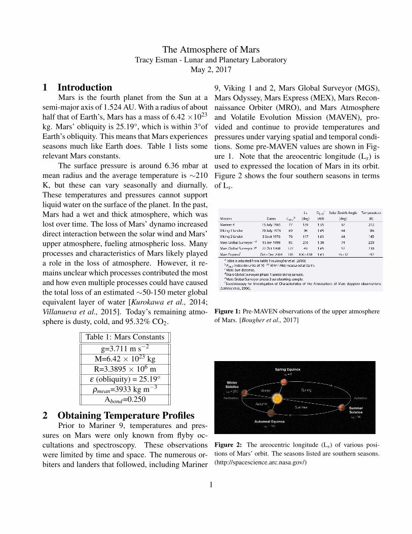
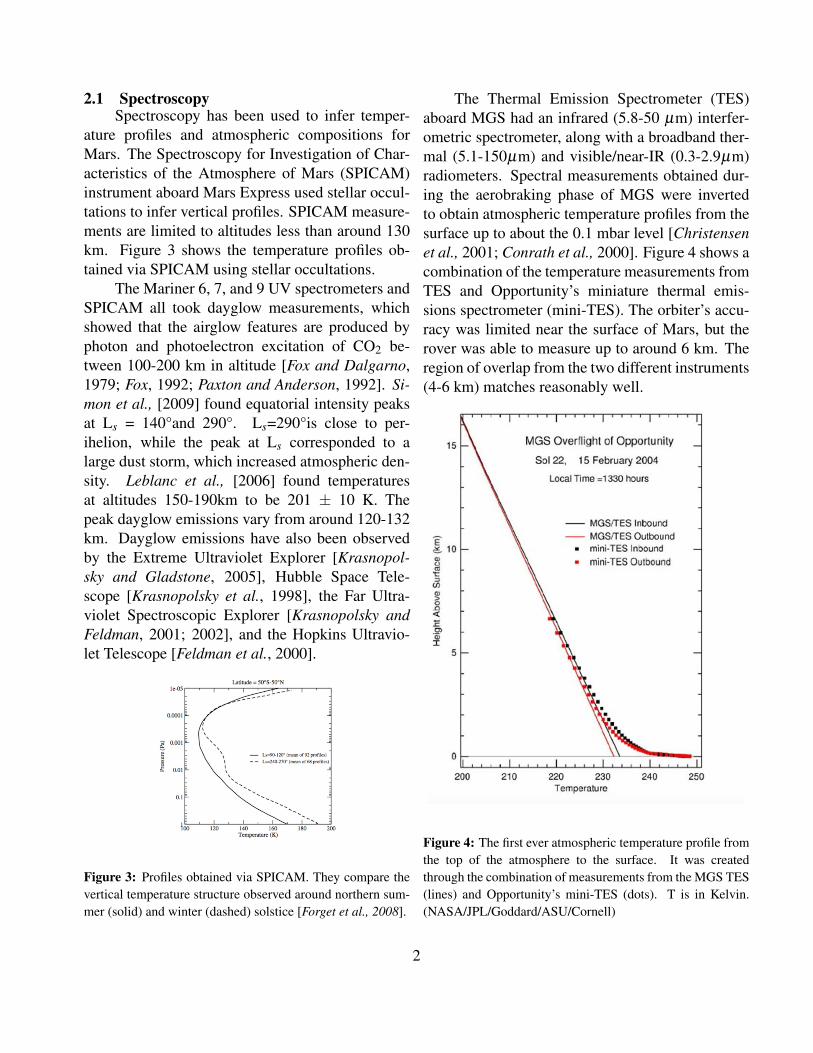
The Atmosphere of MarsTracy Esman - Lunar and Planetary Laboratory

May 2, 2017

1 IntroductionMars is the fourth planet from the Sun at a

semi-major axis of 1.524 AU. With a radius of abouthalf that of Earth’s, Mars has a mass of 6.42 ×1023

kg. Mars’ obliquity is 25.19°, which is within 3°ofEarth’s obliquity. This means that Mars experiencesseasons much like Earth does. Table 1 lists somerelevant Mars constants.

The surface pressure is around 6.36 mbar atmean radius and the average temperature is ∼210K, but these can vary seasonally and diurnally.These temperatures and pressures cannot supportliquid water on the surface of the planet. In the past,Mars had a wet and thick atmosphere, which waslost over time. The loss of Mars’ dynamo increaseddirect interaction between the solar wind and Mars’upper atmosphere, fueling atmospheric loss. Manyprocesses and characteristics of Mars likely playeda role in the loss of atmosphere. However, it re-mains unclear which processes contributed the mostand how even multiple processes could have causedthe total loss of an estimated ∼50-150 meter globalequivalent layer of water [Kurokawa et al., 2014;Villanueva et al., 2015]. Today’s remaining atmo-sphere is dusty, cold, and 95.32% CO2.

Table 1: Mars Constantsg=3.711 m s−2

M=6.42 × 1023 kgR=3.3895 × 106 m

ε (obliquity) = 25.19°ρmean=3933 kg m−3

Abond=0.250

2 Obtaining Temperature ProfilesPrior to Mariner 9, temperatures and pres-

sures on Mars were only known from flyby oc-cultations and spectroscopy. These observationswere limited by time and space. The numerous or-biters and landers that followed, including Mariner

9, Viking 1 and 2, Mars Global Surveyor (MGS),Mars Odyssey, Mars Express (MEX), Mars Recon-naissance Orbiter (MRO), and Mars Atmosphereand Volatile Evolution Mission (MAVEN), pro-vided and continue to provide temperatures andpressures under varying spatial and temporal condi-tions. Some pre-MAVEN values are shown in Fig-ure 1. Note that the areocentric longitude (Ls) isused to expressed the location of Mars in its orbit.Figure 2 shows the four southern seasons in termsof Ls.

Figure 1: Pre-MAVEN observations of the upper atmosphereof Mars. [Bougher et al., 2017]

Figure 2: The areocentric longitude (Ls) of various posi-tions of Mars’ orbit. The seasons listed are southern seasons.(http://spacescience.arc.nasa.gov/)

1

2.1 SpectroscopySpectroscopy has been used to infer temper-

ature profiles and atmospheric compositions forMars. The Spectroscopy for Investigation of Char-acteristics of the Atmosphere of Mars (SPICAM)instrument aboard Mars Express used stellar occul-tations to infer vertical profiles. SPICAM measure-ments are limited to altitudes less than around 130km. Figure 3 shows the temperature profiles ob-tained via SPICAM using stellar occultations.

The Mariner 6, 7, and 9 UV spectrometers andSPICAM all took dayglow measurements, whichshowed that the airglow features are produced byphoton and photoelectron excitation of CO2 be-tween 100-200 km in altitude [Fox and Dalgarno,1979; Fox, 1992; Paxton and Anderson, 1992]. Si-mon et al., [2009] found equatorial intensity peaksat Ls = 140°and 290°. Ls=290°is close to per-ihelion, while the peak at Ls corresponded to alarge dust storm, which increased atmospheric den-sity. Leblanc et al., [2006] found temperaturesat altitudes 150-190km to be 201 ± 10 K. Thepeak dayglow emissions vary from around 120-132km. Dayglow emissions have also been observedby the Extreme Ultraviolet Explorer [Krasnopol-sky and Gladstone, 2005], Hubble Space Tele-scope [Krasnopolsky et al., 1998], the Far Ultra-violet Spectroscopic Explorer [Krasnopolsky andFeldman, 2001; 2002], and the Hopkins Ultravio-let Telescope [Feldman et al., 2000].

Figure 3: Profiles obtained via SPICAM. They compare thevertical temperature structure observed around northern sum-mer (solid) and winter (dashed) solstice [Forget et al., 2008].

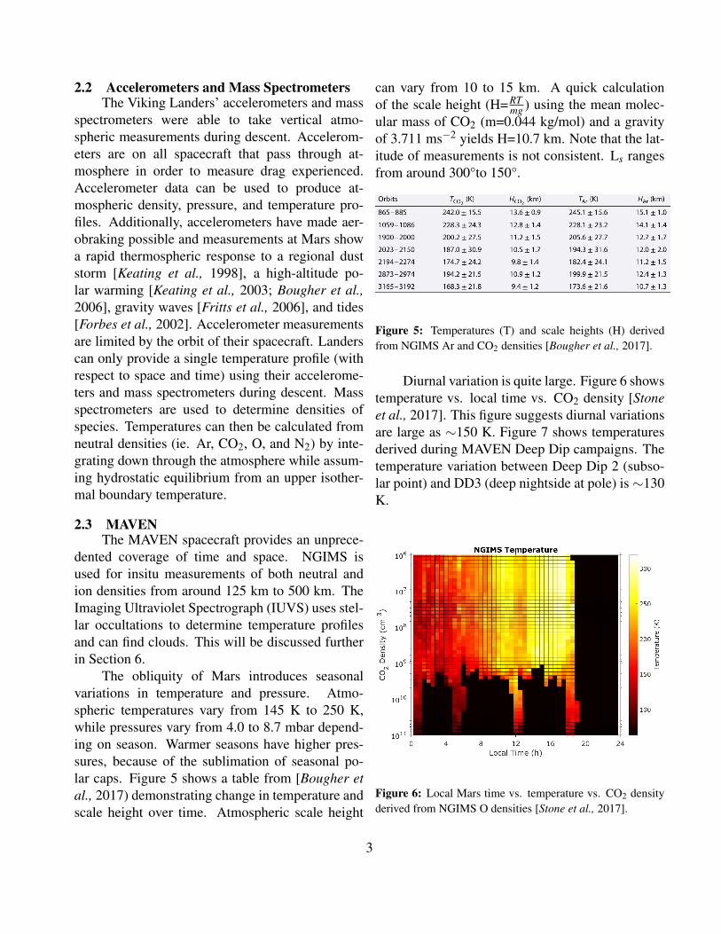
The Thermal Emission Spectrometer (TES)aboard MGS had an infrared (5.8-50 µm) interfer-ometric spectrometer, along with a broadband ther-mal (5.1-150µm) and visible/near-IR (0.3-2.9µm)radiometers. Spectral measurements obtained dur-ing the aerobraking phase of MGS were invertedto obtain atmospheric temperature profiles from thesurface up to about the 0.1 mbar level [Christensenet al., 2001; Conrath et al., 2000]. Figure 4 shows acombination of the temperature measurements fromTES and Opportunity’s miniature thermal emis-sions spectrometer (mini-TES). The orbiter’s accu-racy was limited near the surface of Mars, but therover was able to measure up to around 6 km. Theregion of overlap from the two different instruments(4-6 km) matches reasonably well.

Figure 4: The first ever atmospheric temperature profile fromthe top of the atmosphere to the surface. It was createdthrough the combination of measurements from the MGS TES(lines) and Opportunity’s mini-TES (dots). T is in Kelvin.(NASA/JPL/Goddard/ASU/Cornell)

2

2.2 Accelerometers and Mass SpectrometersThe Viking Landers’ accelerometers and mass

spectrometers were able to take vertical atmo-spheric measurements during descent. Accelerom-eters are on all spacecraft that pass through at-mosphere in order to measure drag experienced.Accelerometer data can be used to produce at-mospheric density, pressure, and temperature pro-files. Additionally, accelerometers have made aer-obraking possible and measurements at Mars showa rapid thermospheric response to a regional duststorm [Keating et al., 1998], a high-altitude po-lar warming [Keating et al., 2003; Bougher et al.,2006], gravity waves [Fritts et al., 2006], and tides[Forbes et al., 2002]. Accelerometer measurementsare limited by the orbit of their spacecraft. Landerscan only provide a single temperature profile (withrespect to space and time) using their accelerome-ters and mass spectrometers during descent. Massspectrometers are used to determine densities ofspecies. Temperatures can then be calculated fromneutral densities (ie. Ar, CO2, O, and N2) by inte-grating down through the atmosphere while assum-ing hydrostatic equilibrium from an upper isother-mal boundary temperature.

2.3 MAVENThe MAVEN spacecraft provides an unprece-

dented coverage of time and space. NGIMS isused for insitu measurements of both neutral andion densities from around 125 km to 500 km. TheImaging Ultraviolet Spectrograph (IUVS) uses stel-lar occultations to determine temperature profilesand can find clouds. This will be discussed furtherin Section 6.

The obliquity of Mars introduces seasonalvariations in temperature and pressure. Atmo-spheric temperatures vary from 145 K to 250 K,while pressures vary from 4.0 to 8.7 mbar depend-ing on season. Warmer seasons have higher pres-sures, because of the sublimation of seasonal po-lar caps. Figure 5 shows a table from [Bougher etal., 2017) demonstrating change in temperature andscale height over time. Atmospheric scale height

can vary from 10 to 15 km. A quick calculationof the scale height (H=RT

mg ) using the mean molec-ular mass of CO2 (m=0.044 kg/mol) and a gravityof 3.711 ms−2 yields H=10.7 km. Note that the lat-itude of measurements is not consistent. Ls rangesfrom around 300°to 150°.

Figure 5: Temperatures (T) and scale heights (H) derivedfrom NGIMS Ar and CO2 densities [Bougher et al., 2017].

Diurnal variation is quite large. Figure 6 showstemperature vs. local time vs. CO2 density [Stoneet al., 2017]. This figure suggests diurnal variationsare large as ∼150 K. Figure 7 shows temperaturesderived during MAVEN Deep Dip campaigns. Thetemperature variation between Deep Dip 2 (subso-lar point) and DD3 (deep nightside at pole) is ∼130K.

Figure 6: Local Mars time vs. temperature vs. CO2 densityderived from NGIMS O densities [Stone et al., 2017].

3

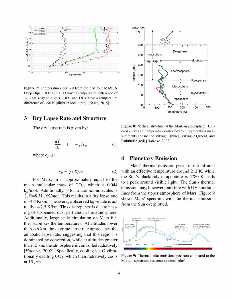
Figure 7: Temperatures derived from the first four MAVENDeep Dips. DD2 and DD3 have a temperature difference of∼130 K (day to night). DD1 and DD4 have a temperaturedifference of ∼90 K (differ in local time). [Stone, 2015]

3 Dry Lapse Rate and StructureThe dry lapse rate is given by:

dTdz

= Γ =−g/cp (1)

where cp is:

cp = γ ∗R/m (2)

For Mars, m is approximately equal to themean molecular mass of CO2, which is 0.044kg/mol. Additionally, γ for triatomic molecules is92 , R=8.31 J/K/mol. This results in a dry lapse rateof -4.4 K/km. The average observed lapse rate is ac-tually ∼-2.5 K/km. This discrepancy is due to heat-ing of suspended dust particles in the atmosphere.Additionally, large scale circulation on Mars fur-ther stabilizes the temperatures. At altitudes lowerthan ∼6 km, the daytime lapse rate approaches theadiabatic lapse rate, suggesting that this region isdominated by convection, while at altitudes greaterthan 15 km, the atmosphere is controlled radiatively[Haberle, 2002]. Specifically, cooling via O vibra-tionally exciting CO2, which then radiatively coolsat 15 µm.

Figure 8: Vertical structure of the Martian atmosphere. Col-ored curves are temperatures inferred from deceleration mea-surements aboard the Viking 1 (blue), Viking 2 (green), andPathfinder (red) [Haberle, 2002].

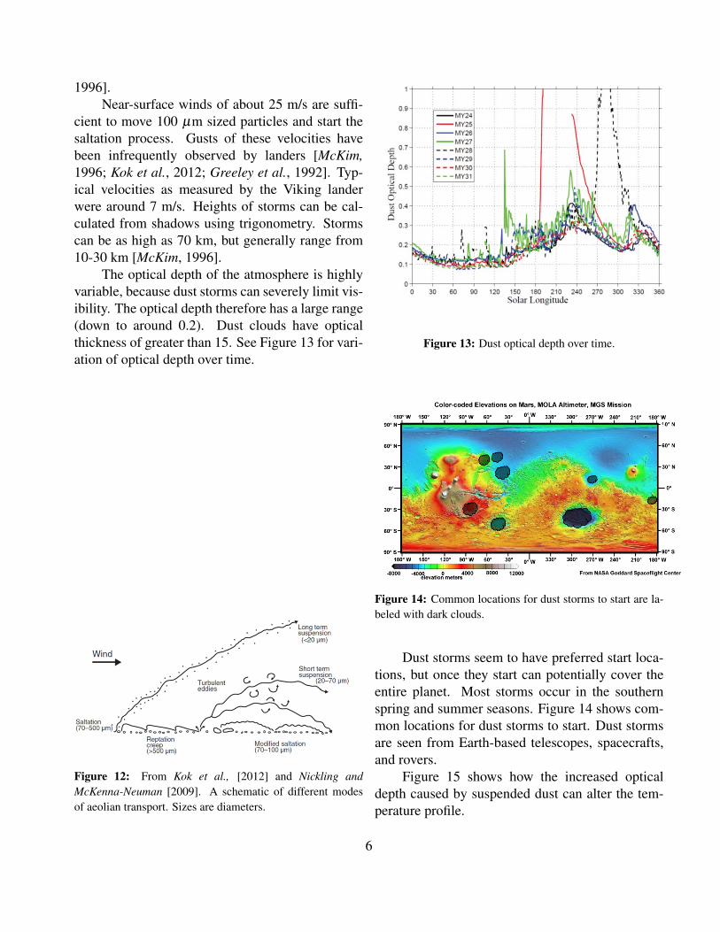
4 Planetary EmissionMars’ thermal emission peaks in the infrared

with an effective temperature around 212 K, whilethe Sun’s blackbody temperature is 5780 K leadsto a peak around visible light. The Sun’s thermalemission may, however, interfere with UV emissionlines from the upper atmosphere of Mars. Figure 9shows Mars’ spectrum with the thermal emissionfrom the Sun overplotted.

Figure 9: Thermal solar emission spectrum compared to theMartian spectrum. (astronomy.nmsu.edu/)

4

5 Atmospheric CompositionThe 5 most abundant gases on Mars are: CO2

(95.32%), N2 (2.7%), Ar (1.6%), O2 (0.13%),and CO (0.08%). Mixing ratios and associ-ated uncertainties are shown in Figure 10.Theabundances were measured by mass spectrometersaboard various spacecraft and landers (most re-cently MAVEN). Mass spectrometers use ionizationto create a beam of ions which can be detected elec-trically. By determining the mass of particles trav-eling through the mass spectrometer, abundances ofspecies can be determined. Some species have ap-proximately the same mass. In order to know theabundances of these certain species, branching ra-tios are needed. If the branching ratio isn’t correct,the abundance won’t be correct. Therefore, sincetrue values for branching ratios are not well-known,some branching ratio number for species must beassumed.

Ions can build-up within the instrument and themeasurements saturate at a maximum value. Alter-natively, if particles get stuck bouncing around in-side the mass spectrometer, sometimes the particlesare falsely detected later on. Corrections also mustbe made for ram pressure at the front of the space-craft and for horizontal movement near periapsis.Figure 11 shows the densities of ions as determinedby NGIMS [Withers et al., 2015]. For many modelsit is sufficient to assume an ionosphere of just O+,O+

2 , and CO+2 .

Figure 10: Atmospheric mixing ratios measured by MSLSAM [Trainer et al., 2014]

Figure 11: Major ion densities in the ionosphere of Mars.The sum of all ion species (dotted) should equal the electrondensity [Withers et al., 2015].

6 Atmospheric Particulates6.1 Dust

The color of Mars and its dust would seemto be a good indicator of the types of mineralsthat can be found suspended in a storm. However,only about 1% of the dust composition is attributedto ferric oxides. At least 60% is silicon dioxide.Overall, the dust storms are composed of a mix-ture of basalt and clay materials. The dust in theair matches well with the surface dust, so has likelybeen lifted into the air and suspended. Smaller par-ticles are likely knocked into the air by the processcalled saltation. Larger particles are lifted up andleap about 10-20cm up and about 1 meter acrossbefore colliding with the surface. The collisionscause dust particles to creep along the surface andsmall gains of diameters <100 µm are dislodged.Particles that leap only short distances before set-tling are being transported through reputation. Outof those particles dislodged from the surface, onlythe particles of <20 µm diameters enter long termsuspension (See Figure 12, which is consistent withobservational evidence for the composition of duststorms. Dust settling time of a major storm of 1971that was observed by Mariner 9 suggests the parti-cles in the storm were 1-10 µm or less in diameter,with an average diameter of around 2 µm [McKim,

5

1996].Near-surface winds of about 25 m/s are suffi-

cient to move 100 µm sized particles and start thesaltation process. Gusts of these velocities havebeen infrequently observed by landers [McKim,1996; Kok et al., 2012; Greeley et al., 1992]. Typ-ical velocities as measured by the Viking landerwere around 7 m/s. Heights of storms can be cal-culated from shadows using trigonometry. Stormscan be as high as 70 km, but generally range from10-30 km [McKim, 1996].

The optical depth of the atmosphere is highlyvariable, because dust storms can severely limit vis-ibility. The optical depth therefore has a large range(down to around 0.2). Dust clouds have opticalthickness of greater than 15. See Figure 13 for vari-ation of optical depth over time.

Figure 12: From Kok et al., [2012] and Nickling andMcKenna-Neuman [2009]. A schematic of different modesof aeolian transport. Sizes are diameters.

Figure 13: Dust optical depth over time.

Figure 14: Common locations for dust storms to start are la-beled with dark clouds.

Dust storms seem to have preferred start loca-tions, but once they start can potentially cover theentire planet. Most storms occur in the southernspring and summer seasons. Figure 14 shows com-mon locations for dust storms to start. Dust stormsare seen from Earth-based telescopes, spacecrafts,and rovers.

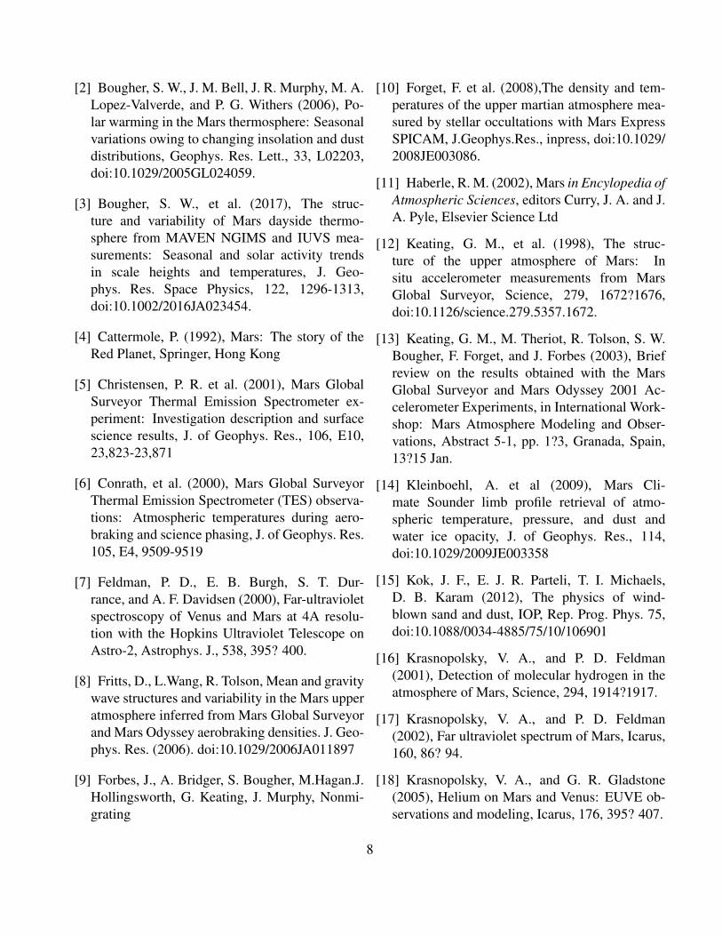
Figure 15 shows how the increased opticaldepth caused by suspended dust can alter the tem-perature profile.

6

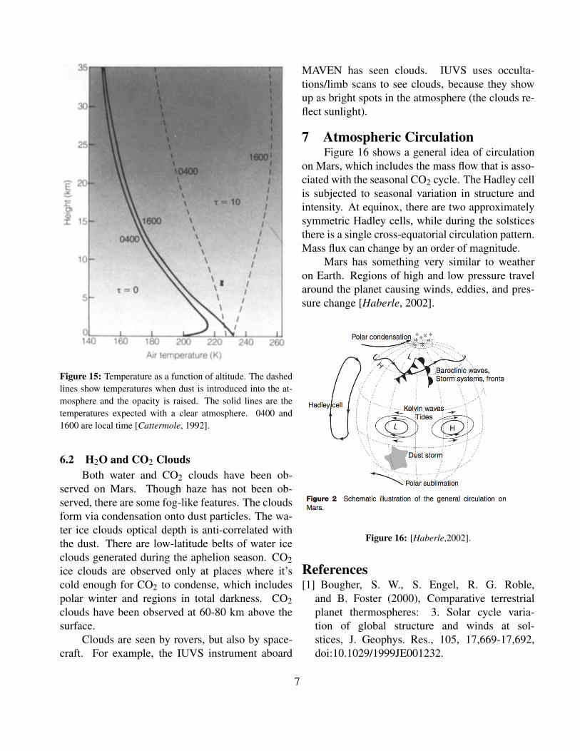
Figure 15: Temperature as a function of altitude. The dashedlines show temperatures when dust is introduced into the at-mosphere and the opacity is raised. The solid lines are thetemperatures expected with a clear atmosphere. 0400 and1600 are local time [Cattermole, 1992].

6.2 H2O and CO2 CloudsBoth water and CO2 clouds have been ob-

served on Mars. Though haze has not been ob-served, there are some fog-like features. The cloudsform via condensation onto dust particles. The wa-ter ice clouds optical depth is anti-correlated withthe dust. There are low-latitude belts of water iceclouds generated during the aphelion season. CO2ice clouds are observed only at places where it’scold enough for CO2 to condense, which includespolar winter and regions in total darkness. CO2clouds have been observed at 60-80 km above thesurface.

Clouds are seen by rovers, but also by space-craft. For example, the IUVS instrument aboard

MAVEN has seen clouds. IUVS uses occulta-tions/limb scans to see clouds, because they showup as bright spots in the atmosphere (the clouds re-flect sunlight).

7 Atmospheric CirculationFigure 16 shows a general idea of circulation

on Mars, which includes the mass flow that is asso-ciated with the seasonal CO2 cycle. The Hadley cellis subjected to seasonal variation in structure andintensity. At equinox, there are two approximatelysymmetric Hadley cells, while during the solsticesthere is a single cross-equatorial circulation pattern.Mass flux can change by an order of magnitude.

Mars has something very similar to weatheron Earth. Regions of high and low pressure travelaround the planet causing winds, eddies, and pres-sure change [Haberle, 2002].

Figure 16: [Haberle,2002].

References[1] Bougher, S. W., S. Engel, R. G. Roble,

and B. Foster (2000), Comparative terrestrialplanet thermospheres: 3. Solar cycle varia-tion of global structure and winds at sol-stices, J. Geophys. Res., 105, 17,669-17,692,doi:10.1029/1999JE001232.

7

[2] Bougher, S. W., J. M. Bell, J. R. Murphy, M. A.Lopez-Valverde, and P. G. Withers (2006), Po-lar warming in the Mars thermosphere: Seasonalvariations owing to changing insolation and dustdistributions, Geophys. Res. Lett., 33, L02203,doi:10.1029/2005GL024059.

[3] Bougher, S. W., et al. (2017), The struc-ture and variability of Mars dayside thermo-sphere from MAVEN NGIMS and IUVS mea-surements: Seasonal and solar activity trendsin scale heights and temperatures, J. Geo-phys. Res. Space Physics, 122, 1296-1313,doi:10.1002/2016JA023454.

[4] Cattermole, P. (1992), Mars: The story of theRed Planet, Springer, Hong Kong

[5] Christensen, P. R. et al. (2001), Mars GlobalSurveyor Thermal Emission Spectrometer ex-periment: Investigation description and surfacescience results, J. of Geophys. Res., 106, E10,23,823-23,871

[6] Conrath, et al. (2000), Mars Global SurveyorThermal Emission Spectrometer (TES) observa-tions: Atmospheric temperatures during aero-braking and science phasing, J. of Geophys. Res.105, E4, 9509-9519

[7] Feldman, P. D., E. B. Burgh, S. T. Dur-rance, and A. F. Davidsen (2000), Far-ultravioletspectroscopy of Venus and Mars at 4A resolu-tion with the Hopkins Ultraviolet Telescope onAstro-2, Astrophys. J., 538, 395? 400.

[8] Fritts, D., L.Wang, R. Tolson, Mean and gravitywave structures and variability in the Mars upperatmosphere inferred from Mars Global Surveyorand Mars Odyssey aerobraking densities. J. Geo-phys. Res. (2006). doi:10.1029/2006JA011897

[9] Forbes, J., A. Bridger, S. Bougher, M.Hagan.J.Hollingsworth, G. Keating, J. Murphy, Nonmi-grating

[10] Forget, F. et al. (2008),The density and tem-peratures of the upper martian atmosphere mea-sured by stellar occultations with Mars ExpressSPICAM, J.Geophys.Res., inpress, doi:10.1029/2008JE003086.

[11] Haberle, R. M. (2002), Mars in Encylopedia ofAtmospheric Sciences, editors Curry, J. A. and J.A. Pyle, Elsevier Science Ltd

[12] Keating, G. M., et al. (1998), The struc-ture of the upper atmosphere of Mars: Insitu accelerometer measurements from MarsGlobal Surveyor, Science, 279, 1672?1676,doi:10.1126/science.279.5357.1672.

[13] Keating, G. M., M. Theriot, R. Tolson, S. W.Bougher, F. Forget, and J. Forbes (2003), Briefreview on the results obtained with the MarsGlobal Surveyor and Mars Odyssey 2001 Ac-celerometer Experiments, in International Work-shop: Mars Atmosphere Modeling and Obser-vations, Abstract 5-1, pp. 1?3, Granada, Spain,13?15 Jan.

[14] Kleinboehl, A. et al (2009), Mars Cli-mate Sounder limb profile retrieval of atmo-spheric temperature, pressure, and dust andwater ice opacity, J. of Geophys. Res., 114,doi:10.1029/2009JE003358

[15] Kok, J. F., E. J. R. Parteli, T. I. Michaels,D. B. Karam (2012), The physics of wind-blown sand and dust, IOP, Rep. Prog. Phys. 75,doi:10.1088/0034-4885/75/10/106901

[16] Krasnopolsky, V. A., and P. D. Feldman(2001), Detection of molecular hydrogen in theatmosphere of Mars, Science, 294, 1914?1917.

[17] Krasnopolsky, V. A., and P. D. Feldman(2002), Far ultraviolet spectrum of Mars, Icarus,160, 86? 94.

[18] Krasnopolsky, V. A., and G. R. Gladstone(2005), Helium on Mars and Venus: EUVE ob-servations and modeling, Icarus, 176, 395? 407.

8

[19] Krasnopolsky, V. A., M. J. Mumma, and G.R. Gladstone (1998), Detection of atomic deu-terium in the upper atmosphere of Mars, Science,280, 1576?1580. Krymskii, A. M., T.

[20] Kurokawa, H., et al., 2014. Evolutionof water reservoirs on Mars: constraintsfrom hydrogen isotopes in martian meteorites.Earth Planet. Sci. Lett. 394, 179-185. doi:10.1016/j.epsl.2014.03.027.

[21] Leblanc, F. et al. (2006), Martian dayglowas seen by the SPICAM UV spectrograph onMars Express, J. of Geophys. Res., 111, E09S11,doi:10.1029/2005JE002664

[22] McCleese, D. J. et al. (2010), Struc-ture and dynamics of the Martian lowerand middle atmosphere as observed by theMars Climate Sounder: Seasonal variations inzonal mean temperature, dust, and water iceaerosols, J. of Geophys. Res., 115, E12016,doi:10.1029/2010JE003677

[23] Nickling, W. G., and C. McKenna Neuman(2009) Aeolian sediment transport Geomorphol-ogy of Desert Environments ed A. Parsons andA. D. Abrahams (New York: Springer) pp 517-555

[24] Paxton, L. J., and D. E. Anderson (1992), Farultraviolet remote sensing of Venus and Mars, inVenus and Mars: Atmospheres, Ionospheres, andSolar Wind Interactions, Geophys. Monogr. Ser.,vol. 66, edited by J. G. Luhmann, M. Tatrallyay,and R. O. Pepin, pp. 113 - 189, AGU, Washing-ton, D. C. Purucker, M., et al. (2000), An

[25] Simon, C. et al. (2009), Dayglow on Mars:Kinetic modeling with SPICAM UV limb data,Planetary and Space Science, 57, 1008-1021,doi: 10.1016/j.pss.2008.08.012

[26] Stone, S. et al. (2017), Private communica-tions, plots for future publications.

[27] Stone, S. et al. (2015), Thermospheric Tem-perature Profiles from NGIMS Deep Dip Data,MAVEN October 2015 PSG presentation

[28] Trainer, M. G. et al. (2014), Seasonal variationof condensable and non-condensable speciesin the gale crater atmosphere as measured bythe MSL SAM instrument, Eighth InternationalConference on Mars, held July 14-18, 2014in Pasadena, California. LPI Contribution No.1791, p.1255

[29] Villanueva, G.L., et al., 2015. Strong waterisotopic anomalies in the martian atmosphere:probing current and ancient reservoirs. Science348, 218-221. doi: 10.1126/science.aaa3630.

[30] Wang, H., and M. I. Richardson (2015),The origin, evolution, and trajectory of largedust storms on Mars during Mars years24-30 (1999-2011), Icarus, 251, 112-127,doi:10.1016/j.icarus.2013.10.033

[31] Withers et al. (2015), Comparison of modelpredictions for the composition of the iono-sphere of Mars to MAVEN NGIMS data, Geo-phys. Res. Letters, 42(21)

9