THE ATLAS OF - Harvard University · tion of The Atlas of Economic Complexity. “The Atlas”, as...
71
THE ATLAS OF
Transcript of THE ATLAS OF - Harvard University · tion of The Atlas of Economic Complexity. “The Atlas”, as...

THE ATLAS OF

A U T H O R S :
Ricardo Hausmann | César A. Hidalgo | Sebastián Bustos Michele Coscia | Alexander Simoes | Muhammed A. Yıldırım
A C K N O W L E D G M E N T S
The research on which this Atlas is based began around 2006 with the idea of the product space. In the original paper published in Science in 2007, we collaborated with Albert-Laszlo Barabasi and Bailey Klinger. The view of economic development of countries as a process of discovering which products a country can master, a process we called self-discovery, came from joint work with Dani Rodrik and later also with Jason Hwang. We explored different implications of the basic approach in papers with Dany Bahar, Bailey Klinger, Robert Lawrence, Francisco Rodriguez, Dani Rodrik, Charles Sabel, Rodrigo Wagner and Andrés Zahler. Throughout, we received significant feedback and advice from Lant Pritchett, Andrés Velasco and Adrian Wood. We would also like to thank Sarah Chung and Juan Jimenez for their contributions to the 2011 edition of The Atlas.
We want to thank the dedicated team that runs Harvard’s Center for International Development (CID) for helping bring The Atlas to life: Marcela Escobari, Jennifer Gala, Andrea Carranza, Melissa Siegel, Victoria Whitney, Adriana Hoyos, Erinn Wattie and Anne Morriss. We are also indebted to the NeCSys team at the MIT Media Lab and to Sandy Sener. We thank the leadership at Harvard Kennedy School and the MIT Media Lab who were early enthusiasts of our work. The editorial design of this book was produced by Draft Diseño (www.draft.cl). We would like to especially acknowledge the contributions of Francisca Barros and Draft Diseño team.
All rights reserved.No part of this book may be reproduced in any form by any electronic or mechanical means (including photocopying, recording, or information storage and retrieval) without permission in writing from the publisher.
MIT Press books may be purchased at special quantity discounts for business or sales promotional use. For information, please email [email protected] or write to Special Sales Department, The MIT Press, 55 Hayward Street, Cambridge, MA 02142.
This book was printed and bound in Malaysia.
Library of Congress Cataloging-in-Publication Data.
The atlas of economic complexity: mapping paths to prosperity / edited by Ricardo Hausmann and César A. Hidalgo. p. cmIncludes bibliographical references.ISBN 978-0-262-52542-8 (pbk. : alk. paper)1. Technological innovation—Economic aspects. 2. Industrial management—Economic aspects. 3. Economic development. 4. Gross domestic product. I. Hausmann, Ricardo. II. Hidalgo, César A. (Professor)HC79.T4A85 2013330.1—dc232013010258
10 9 8 7 6 5 4 3 2 1
T H E A T L A S O F E C O N O M I C C O M P L E X I T YM A P P I N G P A T H S T O P R O S P E R I T Y
© 2013 Massachusetts Institute of Technology and Center for International Development, Harvard University

| Ricardo Hausmann | César A. Hidalgo | Sebastián Bustos | | Michele Coscia | Alexander Simoes | Muhammed A. Yıldırım |
The MIT Press, Cambridge, Massachusetts, London, England
THE ATLAS OF


We thank the many individuals who, early on, understood the potential impact of research oneconomic growth, and shared our team’s vision. The generosity of these supporters made this work feasible
and now makes it available to individuals, organizations and governments throughout the world.
T H E A U T H O R S W A N T T O A C K N O W L E D G E T H E G E N E R O U S S U P P O R T O F :
| Alejandro Santo Domingo | Standard Bank | Anonymous Donor |

6 | THE ATLAS OF ECONOMIC COMPLEXITY
t has been two years since we published the first edi-tion of The Atlas of Economic Complexity. “The Atlas”, as we have come to refer to it, has helped extend the availability of tools and methods that can be used to study the productive structure of countries and its evolution.
Many things have happened since the first edition of The Atlas was released at CID’s Global Empower-ment Meeting, on October 27, 2011. The new edition
has sharpened the theory and empirical evidence of how knowhow affects income and growth and how knowhow itself grows over time. In this edition, we also update our numbers to 2010, thus adding two more years of data and extending our projections. We also undertook a major over-haul of the data. Sebastián Bustos and Muhammed Yildirim went back to the original sources and created a new data-set that significantly improves on the one used for the first edition. They developed a new technique to clean the data, reducing inconsistencies and the problems caused by misre-porting. The new dataset provides a more accurate estimate of the complexity of each country and each product. With this improved dataset, our results are even stronger.
The online sister site of this publication, The Atlas online (http://atlas.cid.harvard.edu) has been significantly enhanced with the use of an updated dataset which now covers up to 2011; the addition of bilateral trade data; and the inclusion of trade information classified according to the Harmonized Sys-tem, a recently developed data set which goes back to 1995, as well as the more traditional Standardized International Trade Classification (SITC-4) dating back to 1962. The Atlas online now also includes multilingual support, country profiles, bulk
I
F O R E W O R D T O T H E U P D A T E D E D I T I O N
data downloads, and a large number of design features, includ-ing dynamic text for the Tree Map visualizations and an im-proved design of the Product Space visualizations.
The Atlas online was originally launched as The Observa-tory and was developed by Alex Simoes with the assistance of Crystal Noel. The Atlas online is currently managed by Romain Vuillemot at the Center for International Development at Har-vard University.
All in all, the new versions of The Atlas and its website provide a more accurate picture of each country’s economy, what products are in its “adjacent possible” and its future growth potential.

MAPPING PATHS TO PROSPERITY | 7
ver the past two centuries, mankind has accomplished what used to be unthink-able. When we look back at our long list of achievements, it is easy to focus on the most audacious of them, such as our con-quest of the skies and the moon. Our lives, however, have been made easier and more prosperous by a large number of more modest, yet crucially important feats.
Think of electric bulbs, telephones, cars, personal comput-ers, antibiotics, TVs, refrigerators, watches and water heat-ers. Think of the many innovations that benefit us despite our limited awareness of them, such as advances in port management, electric power distribution, agrochemicals and water purification. This progress was possible because we got smarter. During the past two centuries, there has been an explosion of ‘productive knowledge’, by which we mean, the knowledge that goes into making the products we make. This expansion was not, however, an individual phenomenon. It was a collective phenomenon. As individu-als we are not much more capable than our ancestors, but as societies we have developed the ability to make all that we have mentioned – and much, much more.
A modern society can amass large amounts of productive knowledge because it distributes bits and pieces of knowl-edge among its many members. But to make use of it, this knowledge has to be put back together through organiza-tions and markets. Thus, individual specialization begets diversity at the national and global level. Our most prosper-ous modern societies are wiser, not because their citizens are individually brilliant, but because these societies hold
O
P R E F A C E

8 | THE ATLAS OF ECONOMIC COMPLEXITY
however, is not enough. In order to put knowledge into pro-ductive use, societies need to reassemble these distributed bits through teams, organizations and markets.
Accumulating productive knowledge is difficult. For the most part, it is not available in books or on the Internet. It is embedded in brains and human networks. It is tacit and hard to transmit and acquire. It comes from years of experience more than from years of schooling. Productive knowledge, therefore, cannot be learned easily like a song or a poem. It requires structural changes. Just like learning a language requires changes in the structure of the brain, developing a new industry requires changes in the patterns of interaction inside an organization or society.
Expanding the amount of productive knowledge available in a country involves enlarging the set of activities that the country is able to do. This process, however, is tricky. Indus-tries cannot exist if the requisite productive knowledge is absent, yet accumulating bits of productive knowledge will make little sense in places where the industries that require it are not present. This “chicken and egg” problem slows down the accumulation of productive knowledge. It also creates important path dependencies. It is easier for coun-tries to move into industries that mostly reuse what they already know, since these industries require adding mod-est amounts of productive knowledge. By gradually adding new knowledge to what they already know, countries can economize on the chicken and egg problem. That is why we find empirically that countries move from the products that they already create to others that are “close by” in terms of the productive knowledge that they require.
a diversity of knowhow and because they are able to re-combine it to create a larger variety of smarter and better products.
The social accumulation of productive knowledge has not been a universal phenomenon. It has taken place in some parts of the world, but not in others. Where it has happened, it has underpinned an incredible increase in liv-ing standards. Where it has not, living standards resemble those of centuries past. The enormous income gaps be-tween rich and poor nations are an expression of the vast differences in productive knowledge amassed by different nations. These differences are expressed in the diversity and sophistication of the things that each of them makes, which we explore in detail in this Atlas.
Just as nations differ in the amount of productive knowl-edge they hold, so do products. The amount of knowledge that is required to make a product can vary enormously from one good to the next. Most modern products require more knowledge than what a single person can hold. No-body in this world, not even the savviest geek or the most knowledgeable entrepreneur knows how to make a com-puter from scratch. We all have to rely on others who know about battery technology, liquid crystals, microprocessor de-sign, software development, metallurgy, milling, lean manu-facturing and human resource management, among many other skills. That is why the average worker in a rich coun-try works in a firm that is much larger and more connected than firms in poor countries. For a society to operate at a high level of total productive knowledge, individuals must know different things. Diversity of productive knowledge,

MAPPING PATHS TO PROSPERITY | 9
The Atlas of Economic Complexity attempts to measure the amount of productive knowledge that each country holds. Our measure of productive knowledge can account for the enor-mous income differences between the nations of the world and has the capacity to predict the rate at which countries will grow. In fact, it is much more predictive than other well-known de-velopment indicators, such as those that attempt to measure competitiveness, governance, education and financial depth.
A central contribution of this Atlas is the creation of a map that captures the similarity of products in terms of their knowledge requirements. This map depicts a network of products, and shows paths through which productive knowledge is more easily accumulated. We call this map the product space. Using data on what each country exports, we are able to place where each country’s production is located in the product space, illustrating their current productive capabilities and identifying products that lie nearby.
Ultimately, this Atlas views economic development as a social learning process, but one that is rife with pitfalls and dangers. Countries accumulate productive knowledge by developing the capacity to make a larger variety of products of increasing complexity. This process involves trial and er-ror. It is a risky journey in search of the possible. Entrepre-neurs, investors and policymakers play a fundamental role in this economic exploration.
By providing rankings, we wish to clarify the scope of the achievable, as revealed by the experience of others. By track-ing progress, we offer feedback regarding current trends. By providing maps, we do not pretend to tell potential prod-uct space explorers where to go, but to pinpoint what is out there and what routes may be shorter or more secure. We hope this will empower these explorers with valuable infor-mation that will encourage them to take on the challenge and thus speed up the process of economic development.
Director, Center for International Development at Harvard University,Professor of the Practice of Economic Development, Harvard Kennedy School,George Cowan Professor, Santa Fe Institute.
ABC Career Development Professor, MIT Media Lab,Massachusetts Institute of Technology (MIT),Faculty Associate, Center for International Development at Harvard University.
R I C A R D O H A U S M A N N C É S A R A . H I D A L G O

What Do We Mean by Economic Complexity?
How Do We Measure Economic Complexity?
Why Is Economic Complexity Important?
How Is Complexity Different from Other Approaches?
How Does Economic Complexity Evolve?
How Can This Atlas Be Used?
Which Countries Are Included in This Atlas?
14
50
26
68
19
64
34
S E C T I O N 1
S E C T I O N 2
S E C T I O N 3
S E C T I O N 4
S E C T I O N 5
S E C T I O N 6
S E C T I O N 7
WHAT, WHY AND HOW? P A R T 1
C O N T E N T S

How to Read the Country Pages
Albania
Zimbabwe
104
Economic Complexity Index
Complexity Outlook Index
Expected Growth in Per Capita GDP to 2020
Expected GDP Growth to 2020
Change in Economic Complexity (1964-2010)
72
96
8478
90
R A N K I N G 1
R A N K I N G 2
R A N K I N G 3
R A N K I N G 4
R A N K I N G 5
108···
358
COMPLEXITY RANKINGS P A R T 2
COUNTRY PAGES P A R T 3

WHAT, WHY AND HOW? P A R T 1


What Do We Mean by Economic Complexity?
S E C T I O N 1

MAPPING PATHS TO PROSPERITY | 15
ne way of describing the economic world is to say that the things we make require machines, raw materials and labor. An-other way is to emphasize that products are made with knowledge. Consider tooth-paste. Is toothpaste just some paste in a tube? Or do the paste and the tube allow us to access knowledge about the properties of sodium fluoride on teeth and about how
to achieve its synthesis? The true value of a tube of tooth-paste, in other words, is that it manifests knowledge about the chemicals that kill the germs that cause bad breath, cavities and gum disease.
When we think of products in these terms, markets take on a different meaning. Markets allow us to access the vast amounts of knowledge that are scattered among the people of the world. Toothpaste represents knowledge about the chemicals that prevent tooth decay, just like cars embody our knowledge of mechanical engineering, metallurgy, elec-tronics and design. Next time you bite into an apple, consid-er that thousands of years of plant domestication has been combined with knowledge about logistics, refrigeration, pest control, food safety and the preservation of fresh produce to bring you that piece of fruit. Products are vehicles for knowl-edge, and the process of embedding knowledge in products requires people who possess a working understanding of that knowledge. Most of us have no idea how toothpaste works, let alone how to make it, because we can rely on the few people who know how to create this molecular cocktail, and who, together with their colleagues at the toothpaste factory, can create a product that we use every day.
OWe owe to Adam Smith the idea that the division of labor
is the secret of the wealth of nations. In a modern reinter-pretation of this idea, the reason why the division of labor is powerful is that it allows us to access a quantity of knowl-edge that none of us would be able to hold individually. We rely on dentists, plumbers, lawyers, meteorologists and car mechanics to sustain our standard of living, because few of us know how to fill cavities, repair leaks, write contracts, predict the weather or fix our cars. Markets and organiza-tions allow the knowledge that is held by few to reach many. In other words, they make us collectively wiser.
The amount of knowledge embedded in a society, how-ever, does not depend mainly on how much knowledge each individual holds. It depends, more fundamentally on the diversity of knowledge across individuals and on their abil-ity to combine this knowledge, and make use of it, through complex webs of interaction. A hunter-gatherer in the Arctic must know a lot of things to survive. Without the knowledge held by each member of an Inuit community, most people unfamiliar with the Arctic would die. While the knowledge held by each individual, or within each family, is essential for survival and wellbeing, the total amount of knowledge embedded in a hunter-gatherer society is not very different from that which is embedded in each one of its members. The secret of modern societies is not that each person holds much more productive knowledge than those in a more tra-ditional society. The secret to modernity is that we collec-tively use large volumes of knowledge, while each one of us holds only a few bits of it. Society functions because its members form webs that allow them to specialize and share their knowledge with others.
We can distinguish between two kinds of knowledge: ex-plicit and tacit. Explicit knowledge can be transferred easily by reading a text or listening to a conversation. Yesterday’s sports results, tomorrow’s weather forecast or the size of the moon can all be learned quickly by looking them up in a newspaper or on the web. And yet, if all knowledge had this characteristic, the world would be very different. Countries would catch up very quickly to frontier technologies, and the income differences across the world would be much smaller than those we see today. The problem is that crucial parts of knowledge are tacit and therefore hard to embed in people. Learning how to fix dental problems, speak a foreign language, or run a farm requires a costly and time-consuming effort. As a consequence, it does not make sense for all of us to spend our lives learning how to do everything. Because it is hard to transfer, tacit knowledge is what constrains the process of growth and development. Ultimately, differences in prosper-ity are related to the amount of tacit knowledge that societies hold and to their ability to combine and share this knowledge.
Because embedding tacit knowledge is a long and costly process, we specialize. This is why people are trained for specific occupations and why organizations become good at specific functions. To fix cavities you must be able to iden-tify them, remove the decayed material and fill the hole. To play baseball, you must know how to catch, field and bat, but you do not need to know how to give financial advice or fix cavities. On the other hand, to perform the function of
baseball player, knowing how to catch a ball is not enough (you must also be able to field and bat). In other words, in al-locating productive knowledge to individuals, it is important that the chunks each person gets be internally coherent so that he or she can perform a certain function. We refer to these modularized chunks of embedded knowledge as capa-bilities. Some of these capabilities have been modularized at the level of individuals, while others have been grouped into organizations and even into networks of organizations.
For example, consider what has happened with under-graduate degrees, which in the United States require four years of study. This norm has remained constant for the last four centuries. During the same period, however, knowledge has expanded enormously. The university system did not respond to the increase in knowledge by lengthening the time it takes to get a college degree. Instead, it increased the diversity of degrees. What used to be a degree in philoso-phy was split into natural and moral philosophy, the former later splitting into physics, chemistry and biology and later into other disciplines such as ecology, earth sciences and genetics. The Bureau of Labor Statistics’ Standard Occupa-tion Classification for 2010 lists 840 different occupations, including 78 in healthcare, 16 in engineering, 35 kinds of sci-entists – in coarse categories such as economists, physicists and chemists, five types of artists, and eight kinds of design-ers. We all certainly can imagine an even more nuanced classification in our respective fields. For instance, we could

distinguish between economists that specialize in labor, trade, finance, development, industrial organization, macro and econometrics, among others. If we did this further dis-aggregation for all occupations, we would easily go into the tens of thousands. The only way that society can hold all of the knowledge we have is by distributing coherent pieces of it among individuals. This is how the world adapts to ex-panding knowledge.
Specialization allows societies to store more knowledge, but the question becomes how to put the different chunks of specialized knowledge to use. Most products that are used to-day require more knowledge than can be mastered by any in-dividual. Hence, those products require that individuals with different capabilities interact with each other. We call the amount of knowledge held by one person a personbyte. How can you make a product that requires the input of 100 differ-ent people, or 100 personbytes? Obviously, it cannot be made by a micro-entrepreneur working alone. It has to be made either by an organization with at least 100 individuals (each with a different personbyte), or by a network of organizations that can aggregate these 100 personbytes of knowledge.
Consider how a shirt is made and sold. It first needs to be designed, and then fabric must be procured, cut and sewn. It needs to be packed, branded, marketed and distributed. In a firm that manufactures shirts, different people will hold expertise in each of these knowledge chunks – the shirt business requires all of them. Moreover, you need to finance
the operation, hire the relevant people, coordinate all the activities and negotiate everybody’s buy-in, which in itself requires different kinds of knowhow. To make shirts, you can import the fabric and, by doing so, access the knowl-edge about looms and threading that is embedded in a piece of cloth. Yet some of the knowledge required cannot be ac-cessed through shipped inputs. The people with the relevant knowledge must be near the place where shirts are made.
This does not begin to list all that is required to make and sell a shirt. To operate efficiently, firms rely on a large set of complementary systems, networks and markets. Raw ma-terials need to be shipped in and the final product shipped out using transportation companies, ports, roads, airplanes or airports. Workers need to get to work and back home us-ing some kind of urban transportation system. Machines need to be powered by electricity and processes need ac-cess to water and water treatment facilities. To be able to operate, the plant manager needs all of these services to be locally available, but she does not need to organize them herself. Other organizations are responsible for organizing and aggregating the personbytes required to generate pow-er, provide clean water, and run a transportation system. The relevant capabilities to perform all of these functions reside in organizations that are able to package the relevant knowledge into transferable bundles. These are bundles of knowhow that are more efficiently organized separately and transferred as intermediate inputs or services. We can think

18 | THE ATLAS OF ECONOMIC COMPLEXITY
of these bundles as organizational capabilities the manu-facturer needs. In fact, just as knowhow is modularized in people in the form of individual capabilities, larger amounts of knowhow are modularized in organizations, and net-works of organizations.
Ultimately, to make the products that have been invented in the past 200 years, many personbytes have to be put to-gether. These different personbytes have to reside in differ-ent people. To utilize the diversity of knowledge in a com-plex society, many people have to come together in many ways. They form teams we call firms and organizations and these are in turn connected through markets and other forms of interaction. The amount of productive knowledge that a society uses is reflected in the variety of firms it has, in the variety of occupations these firms require and in the extent of interactions between firms. Economic complexity is a measure of how intricate this network of interactions is and hence of how much productive knowledge a society mo-bilizes. Economic complexity, therefore, is expressed in the composition of a country’s productive output and reflects the structures that emerge to hold and combine knowledge.
Knowledge can only be accumulated, transferred and preserved if it is embedded in networks of individuals and organizations that put this knowledge into productive use. Knowledge that is not used is not transferred, and will
How Do We Measure Economic Complexity?
disappear once the individuals and organization that have it retire or die.
Said differently, countries do not make all the products and services they use and need. They make the ones they can, using the knowledge embedded in their own people and organizations. Some goods, like medical imaging devices or jet engines, require large amounts of knowledge and are the results of very large networks of people and organiza-tions. By contrast, wood logs or coffee beans require much less knowledge and the networks required to support these operations do not need to be as large. Complex economies are those that can weave vast quantities of relevant knowl-edge together, across large networks of people, to generate a diverse mix of knowledge-intensive products. Simpler economies, in contrast, have a narrower base of productive knowledge and as a result they produce fewer and simpler products, requiring smaller webs of interaction. Because in-dividuals are limited in what they know, the only way so-cieties can expand their knowledge base is by facilitating the interaction of individuals with different knowledge sets in increasingly complex webs of organizations and markets. Increased economic complexity is necessary for a society to be able to hold and use a larger amount of productive knowl-edge. Because of this, we can measure complexity by looking at the mix of products that countries are able to make.

How Do We Measure Economic Complexity?S E C T I O N 2

20 | THE ATLAS OF ECONOMIC COMPLEXITY
s we have argued, productive knowledge is the key to prosperity. Larger amounts of pro-ductive knowledge require increasingly com-plex webs of human interaction, which we call economic complexity. In this Section we develop measures of the amount of produc-tive knowledge held by different societies. How can we go about doing this, given that there are no direct ways to look at a country
and know how much knowledge is embedded in it? Our ap-proach is based on the following trick: we can look at what countries make, and from this, we can begin to infer what a country knows.
We can observe how many different kinds of products a country is able to make. We call this the diversity of a coun-try (Figure 2.1). We can also observe the number of countries that are able to make a product. We call this the ubiquity of a product (Figure 2.1). We assume that countries are only able to make the products for which they have the requisite knowledge. From this simple claim, it is possible to extract a few implications that can be used to construct a measure of economic complexity.
The game of Scrabble is a useful analogy. In Scrabble, players use tiles containing single letters to make words. For instance, a player can use the tiles A, C and R to con-struct the words CAR or ARC. In this analogy, words are like products and letters are like capabilities, or modules of em-bedded knowledge. We assume that each player has plenty of copies of the letters that they do have. This means that if a country has a certain module of knowledge, it can use that knowledge in many different settings. Our challenge is to measure the number of different letters the players have by looking at two things: first, the number of words that each player can write; second, the number of players who can write a particular word.
Players who have more letters should be able to make more words. We can expect the diversity of words (products)
Athat players (countries) can make to be strongly related to the number of letters (capabilities) that they have. Hence, diversity is a first measure of how much knowledge a country has.
Let us look now at words. The number of players who can make a word is indicative of how many letters the word has. Longer words will tend to be less common, since they can only be put together by players who have all the requisite letters. Similarly, more complex products will be less com-mon because only the countries that have all the requisite knowledge will be able to make them. Products that require little knowledge should be more ubiquitous and vice versa.
The diversity of a country’s exports is a crude approxima-tion of the variety of capabilities available in the country, just as the ubiquity of a product is a crude approximation of the variety of capabilities required by a product. Consider medical imaging devices. These machines are made in few places, and the countries that are able to make them, such as the United States or Germany, also export a large num-ber of other products. From this we can infer that medical imaging devices are complex because few countries make them and those that do tend to be diverse. Now consider the case of raw diamonds. These products are extracted in very few places, making their ubiquity quite low. But is this a re-flection of the high knowledge-intensity of raw diamonds? Not at all! If raw diamonds were complex, then the countries that extract diamonds should also be able to make many other things because they would have the many capabilities required by diamonds. We see though that Sierra Leone and Botswana principally export diamonds. This indicates that, unlike medical imaging devices, something other than large volumes of knowledge makes diamonds rare. Both of these measures are affected by the existence of rare capabilities, which, using the Scrabble analogy, would be represented by letters like Q and X. So, here we have used the diversity of the countries making a product (say, diamonds) to nuance the first impression given by the (low) ubiquity of the product.

MAPPING PATHS TO PROSPERITY | 21
ARGENTINA (ARG)
GHANA (GHA)
X-RAY MACHINES
MEDICAMENTS
CREAMS AND POLISHES
CHEESE
FROZEN FISH
NETHERLANDS (NLD)
F I G U R E 2 . 1 :
U B I Q U I T Y :Ubiquity is related to the number of countries that export a product. This is equal to the number of links that this product has in this network. In this ex-ample, the ubiquity of cheese is 2, that of fish is 3 and that of medicaments is 1.
D I V E R S I T Y :Diversity is related to the number of
products that a country exports. This is equal to the number of links that
this country has in the network that relates countries to the products that
they export. In this example, the di-versity of the Netherlands is 5, that of Argentina is 3, and that of Ghana is 1.
Graphical representation of diversity and ubiquity.
By the same token, we can improve the first impression about the complexity of a country that is given by its di-versity, by also looking at the ubiquity of the products that it makes. Consider a country that chooses to concentrate in a few very complex products. It does so, not because it has few letters, but because it prefers to use them in very long words. Hence, the diversity of the country may give the wrong impression about the availability of capabilities. But if we look at the ubiquity of the products that the coun-try makes, we would see that it specializes in low ubiquity products. We can look further into how diversified the coun-tries that make those products are, and we will find that highly diversified countries make them. The information about how many capabilities the country has is contained not only in the number of products that it makes, but also in the ubiquity of those products and in the diversity of the other countries that make them.
Consider the case of Switzerland and Egypt. The popula-tion of Egypt is 11 times larger than that of Switzerland. At purchasing power prices their GDPs are similar since Swit-zerland is about 8 times richer than Egypt in per capita terms. Under the classification we use in this Atlas, they both export a similar number of different products, about 180. How can products tell us about the conspicuous differ-
ences in the level of development that exist between these two countries? Egypt exports products that are on average exported by 28 other countries (placing Egypt in the 60th percentile of countries in terms of the average ubiquity of its products), while Switzerland exports products that are exported on average by only 19 other countries, putting it in the 5th percentile. Moreover, the products that Switzer-land exports are exported by highly diversified countries, while those that Egypt exports are exported by poorly di-versified countries. Our mathematical approach exploits these second, third and higher order differences to cre-ate measures that approximate the amount of produc-tive knowledge held in each of these countries. Because of these differences, Switzerland is ranked way above Egypt in productive knowledge (Switzerland is ranked 3rd, and Egypt is ranked 67th out of 128 countries in year 2010). Ultimately, what countries make reveals what they know.
This example illustrates that we can improve the esti-mate of the productive knowledge of a country that we in-fer from its diversity by looking at the ubiquity of the prod-ucts that it makes. We can refine it further by looking at the diversity of the countries that make those products and at the ubiquity of the products that those countries make. Similarly, we can improve the estimate of the productive
22 | THE ATLAS OF ECONOMIC COMPLEXITY
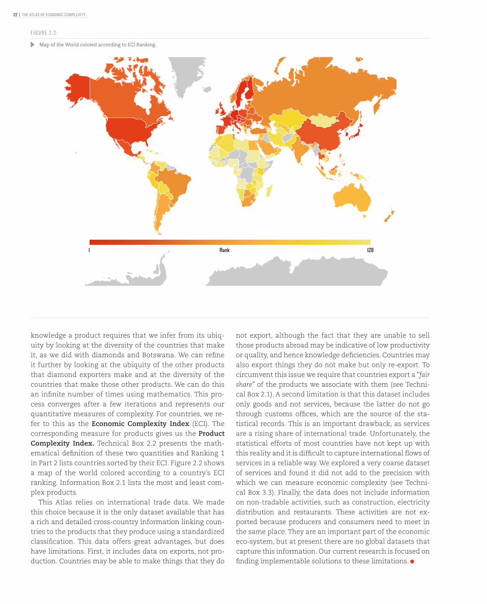
knowledge a product requires that we infer from its ubiq-uity by looking at the diversity of the countries that make it, as we did with diamonds and Botswana. We can refine it further by looking at the ubiquity of the other products that diamond exporters make and at the diversity of the countries that make those other products. We can do this an infinite number of times using mathematics. This pro-cess converges after a few iterations and represents our quantitative measures of complexity. For countries, we re-fer to this as the Economic Complexity Index (ECI). The corresponding measure for products gives us the Product Complexity Index. Technical Box 2.2 presents the math-ematical definition of these two quantities and Ranking 1 in Part 2 lists countries sorted by their ECI. Figure 2.2 shows a map of the world colored according to a country’s ECI ranking. Information Box 2.1 lists the most and least com-plex products.
This Atlas relies on international trade data. We made this choice because it is the only dataset available that has a rich and detailed cross-country information linking coun-tries to the products that they produce using a standardized classification. This data offers great advantages, but does have limitations. First, it includes data on exports, not pro-duction. Countries may be able to make things that they do
not export, although the fact that they are unable to sell those products abroad may be indicative of low productivity or quality, and hence knowledge deficiencies. Countries may also export things they do not make but only re-export. To circumvent this issue we require that countries export a “fair share” of the products we associate with them (see Techni-cal Box 2.1). A second limitation is that this dataset includes only goods and not services, because the latter do not go through customs offices, which are the source of the sta-tistical records. This is an important drawback, as services are a rising share of international trade. Unfortunately, the statistical efforts of most countries have not kept up with this reality and it is difficult to capture international flows of services in a reliable way. We explored a very coarse dataset of services and found it did not add to the precision with which we can measure economic complexity (see Techni-cal Box 3.3). Finally, the data does not include information on non-tradable activities, such as construction, electricity distribution and restaurants. These activities are not ex-ported because producers and consumers need to meet in the same place. They are an important part of the economic eco-system, but at present there are no global datasets that capture this information. Our current research is focused on finding implementable solutions to these limitations.
F I G U R E 2 . 2 :
1 128Rank
Map of the World colored according to ECI Ranking.

MAPPING PATHS TO PROSPERITY | 23
I N F O R M AT I O N B O X 2 . 1 : T H E W O R L D ’ S M O S T A N D L E A S T C O M P L E X P R O D U C T S
T A B L E 2 . 1 . 1 : T O P 5 P R O D U C T S B Y C O M P L E X I T Y
Product Code (SITC4) Product Name Product Community Product Complexity Index
7367 Other machine tools for working metal or metal carbide Machinery 2.08
8744 Instrument & appliances for physical or chemical analysis Chemicals & Health 2.02
7742 Appliances based on the use of X-rays or radiation Chemicals & Health 1.96
8821 Chemical products and flashlight materials for use in photography Chemicals & Health 1.91
7373 Welding, brazing, cutting, etc. machines and appliances, parts, N.E.S. Machinery 1.86
T A B L E 2 . 1 . 2 : B O T T O M 5 P R O D U C T S B Y C O M P L E X I T Y
Product Code (SITC4) Product Name Product Community Product Complexity Index
2631 Raw cotton, excluding linters, not carded or combed Cotton, rice, soy beans and others -2.51
2876 Tin ores and concentrates Mining -2.57
2320 Natural rubber latex; natural rubber and gums Tropical tree-crops and flowers -2.63
2225 Sesame seeds Cotton, rice, soy beans and others -2.99
0721 Cocoa beans, raw, roasted Tropical tree-crops and flowers -3.10
Table 2.1.1 and Table 2.1.2 show respectively the products that rank highest and lowest in the complexity scale. The difference between the world’s most and less complex products is stark. The most complex products are sophisticated chemicals and machinery that tend to emerge from organizations where a large number of high skilled individuals participate. The world’s least complex prod-
ucts, on the other hand, are raw minerals or simple agricultural products.The economic complexity of a country is connected intimately to the complex-ity of the products that it exports. Ultimately, countries can only increase their score in the Economic Complexity Index by becoming competitive in an increas-ing number of complex industries.

24 | THE ATLAS OF ECONOMIC COMPLEXITY
T E C H N I C A L B O X 2 . 1 : M E A S U R I N G E C O N O M I C C O M P L E X I T Y :
Consider , as a matrix in which rows represent different countries and col-umns represents different products. An element of the matrix is equal to 1 if country c produces product p, and 0 otherwise. We can measure diversity and ubiquity simply by summing over the rows or columns of that matrix. Formally, we define:
To generate a more accurate measure of the number of capabilities available in a country, or required by a product, we need to correct the information that diversity and ubiquity carry by using each one to correct the other. For coun-tries, this requires us to calculate the average ubiquity of the products that it exports, the average diversity of the countries that make those products and so forth. For products, this requires us to calculate the average diversity of the countries that make them and the average ubiquity of the other products that these countries make. This can be expressed by the recursion:
We then insert (4) into (3) to obtain
and rewrite this equation as:
We note that (7) is satisfied when . This corresponds to the eigenvector of which is associated with the largest eigenvalue. Since this eigenvector is a vector of ones, it is not informative. We look, instead, for the eigenvector associated with the second largest eigenvalue. This is the ei-genvector that captures the largest amount of variance in the system and is our measure of economic complexity. Hence, we define the Economic Complexity Index (ECI) as:
where
where < > represents an average, and stdev stands for the standard devia-tion and
Analogously, we define a Product Complexity Index (PCI). Because of the symmetry of the problem, this can be done simply by exchanging the index of countries (c) with that for products (p) in the definitions above. Hence, we de-fine PCI as:
where

MAPPING PATHS TO PROSPERITY | 25
We use this measure to construct a matrix that connects each country to the products that it makes. The entries in the matrix are 1 if country c exports product p with Revealed Comparative Advantage larger than 1, and 0 otherwise. Formally we define this as the matrix, where
is the matrix summarizing which country makes what, and is used to construct the product space and our measures of economic complexity for countries and products. In our research we have played around with cutoff values other than 1 to construct the matrix and found that our results are robust to these changes.
Going forward, we moderate changes in export values induced by fluctua-tions in commodity prices by using a modified definition of RCA in which the denominator is averaged over the previous three years.
T E C H N I C A L B O X 2 . 2 : W H O M A K E S W H AT ?
When associating countries to products it is important to take into account the size of the export volume of countries and the world trade in each product. This is because, even for the same product, we expect the volume of exports of a large country like China, to be larger than the volume of exports of a small coun-try like Uruguay. By the same token, we expect the export volume of products that represent a large fraction of world trade, such as cars or footwear, to repre-sent a larger share of a country’s exports than products that account for a small fraction of world trade, like cotton seed oil or potato flour.
To make countries and products comparable we use Balassa’s definition of Revealed Comparative Advantage or RCA. Balassa’s definition says that a coun-try has Revealed Comparative Advantage in a product if it exports more than its “fair share”, that is, a share that is equal to the share of total world trade that the product represents. For example, in 2010, with exports of $42 billion, soy-beans represented 0.35% of world trade. Of this total, Brazil exported nearly $11 billion, and since Brazil’s total exports for that year were $140 billion, soybeans accounted for 7.8% of Brazil’s exports. This represents around 22 times Brazil’s “fair share” of soybean exports (7.8% divided by 0.35%), so we can say that Brazil has a high revealed comparative advantage in soybeans.
Formally, if represents the exports of product by country , we can express the Revealed Comparative Advantage that country has in product as:

Why Is Economic Complexity Important?
S E C T I O N 3

MAPPING PATHS TO PROSPERITY | 27
conomic complexity reflects the amount of knowledge that is embedded in the produc-tive structure of an economy. Seen this way, it is no coincidence that there is a strong correlation between our measures of eco-nomic complexity and the income per cap-ita that countries are able to generate. Fig-ure 3.1 illustrates the relationship between the Economic Complexity Index (ECI) and
income per capita for the 128 countries studied in this Atlas. In this graph, we separate countries according to their intensity in natural resource exports. We color in red those countries for which natural resource exports, such as minerals, gas and oil, represent at least 10% of GDP. For the 75 countries with a limited relative presence of natural-resource exports (in blue), economic complex-ity accounts for 78 percent of the variance in income per capita. But as the Figure 3.1 illustrates, countries with a large presence of natural resources can be relatively rich without being complex. It is easy to see why. But if we take into account the income that is generated from extractive activities, which has more to do with geology than know-how, economic complexity can explain about 78 percent of the variation in income across all 128 countries. Figure 3.2 shows the tight relationship between economic com-plexity and income per capita that emerges after we take into account a country’s natural resource income. The more complex your economy, the more likely you are to have a higher level of income.
Economic complexity, therefore, is related to a country’s level of prosperity. As such, it is just a correlation of things
Ewe care about. The relationship between income and com-plexity, however, goes deeper than this. To see this, note that this relationship is tight but not perfect. As we said before, ECI accounts for 78 percent of the variance, not 100 percent. Countries are not on the red line of Figure 3.2. Some coun-tries are above this line and others are below. Are these gaps just a mistake of the theory or do they contain information about where countries are going? Take, for example, the case of India. Given how much it knows, we would have expected India to be richer. Well, maybe India should be richer. If so, India’s recent rapid growth would be caused by the fact that the country already possesses the knowledge to be richer than it is and is, therefore, moving to “where it belongs” in the regression line. Take by contrast the case of Greece. Our approach would say that Greece is too rich for the little knowledge it has. Well, maybe Greece cannot sustain its re-cent level of income, which has been propped up artificially through massive borrowing that has proven unsustainable: the country is now rapidly moving to “where it belongs”, but in the case of Greece it is in the opposite direction of that of India. Countries whose economic complexity is greater than what we would expect, given their current level of income, tend to grow faster than those that are “too rich” for their current level of economic complexity. Figure 3.3 shows the relationship between the gaps between of ECI and income in 2000 and growth in the decade 2000-2010. The relationship is strong and statistically significant: the gaps between a country’s income and its complexity do tend to be closed in the future through differential growth. In this sense, economic complexity is not just a symptom or an expression of prosperity: it is a driver.

28 | THE ATLAS OF ECONOMIC COMPLEXITY
Shows the relationship between economic complexity and income per capita obtained after controlling for each country’s natural resource exports. After including this control, through the inclusion of the log of natural resource exports per capita, economic complexity and natural resources explain 78% of the variance in per capita income across countries.
F I G U R E 3 . 2 :
Shows the relationship between income per capita and the Economic Complexity Index (ECI) for countries where natural resource exports are larger than 10% of GDP (red) and for those where natural resource exports are lower than 10% of GDP (blue). For the latter group of countries, the Economic Complexity Index accounts for 78% of the variance, a variable commonly known as R2. Countries in which the levels of natural resource exports is relatively high tend to be significantly richer than what would be expected given the complexity of their economies, yet the ECI still correlates strongly with income for that group.
F I G U R E 3 . 1 :
AGO
AREAUS
AZE
BOL
BWA
CHL
COG
DZA
ECU
GAB
GIN
KAZ
KWT
LAO
LBR
MNG
MOZ
MRT
NAM
NGA
NOR
OMN
PER
PNG
QAT
RUS
SAU
SDN
TJK
TTOVEN
YEM
ZAF
ZMB
ALB
ARG
AUTBEL
BGD
BGR
BIH
BLR
BRA
CAN
CHE
CHN
CIVCMR
COLCRI
CZE
DEU
DNK
DOM
EGY
ESP
EST
ETH
FIN
FRA GBR
GEOGHA
GRC
GTM
HKG
HND
HRV HUN
IDN
IND
IRL
ISRITA
JAM JOR
JPN
KENKGZ
KHM
KOR
LBN
LKA
LTULVA
MAR
MDA
MDG
MEX
MKD
MLI
MUS
MWI
MYS
NIC
NLDNZL
PAK
PAN
PHL
POL
PRT
PRY
ROM
SEN
SGP
SLV
SRB
SVK
SVN
SWE
SYR THATKM TUN
TUR
TZA UGA
UKR
URY
USA
UZB VNM
ZWE
68
1012
−2 −1 0 1 2
GDP p
er ca
pita,
log [2
010]
GDP p
er ca
pita,
log /c
ontro
ls

MAPPING PATHS TO PROSPERITY | 29
Technical Box 3.1 shows the statistical evidence that sup-ports our claim that economic complexity precedes and hence drives long run levels of income and consequently growth. The analysis uses a country’s initial level of eco-nomic complexity to predict growth over the subsequent decade, after controlling for initial income and the rise in natural resource exports over the decade.
The ability of the ECI to predict future economic growth suggests that countries tend to move towards an income level that is compatible with their overall level of productive knowledge. On average, their income tends to reflect their embedded knowledge. But when it does not, as the cases of India and Greece illustrate, it gets corrected over time through accelerated or diminished growth.
Over time economic complexity evolves: countries ex-pand their productive capabilities and begin to make more and more complex products. This process will be studied at greater length in Section 5, but for now consider that mak-ing a product that is new to a country requires the addi-tion of all missing capabilities. Adding a product for which a country needs many new capabilities often proves difficult because it requires solving a complicated “chicken and egg” problem. An industry may not exist because the produc-tive capabilities it requires may not be present. But there will be scant incentives to develop the productive capabili-ties required by industries that do not exist. Furthermore, developing those capabilities will be difficult because there is nobody in the country from which to learn the requisite know-how. Because of this problem, countries tend to pref-erentially develop products for which most of the requisite productive capabilities are already present, leaving fewer
“chicken and egg” problems to be solved. We say that these products are “nearby” in terms of productive capabilities.
What differs between countries is the abundance of prod-ucts that they do not yet make but that are near their cur-rent endowment of capabilities. Countries with an abun-dance of such nearby products will find it easier to deal with the chicken and egg problem of coordinating the acquisition of missing capabilities with the development of the indus-tries that demand them. This should allow them to find an easier path towards capability acquisition, product diversi-fication and development. Countries with few nearby prod-ucts will find it hard to acquire more capabilities and hence to increase their economic complexity.
In Section 5 we will show how we measure the abundance of products that are near a country’s current set of produc-tive capabilities. We call it the Complexity Outlook Index (COI). This variable is based on the distance between the products that a country is currently making and those that it is not, weighted by the complexity of the products it is not making. Being near a complex product is worth more than being near a simple product, and being near is worth more than being far.
We show the Complexity Outlook Index plotted against the Economic Complexity Index in Figure 3.4. The graph shows an inverted U shape. Countries with low ECI (those with few capabilities) find most products very “far” and opportunities very limited. This is reflected in a low COI. Countries with a high ECI are highly diversified: they al-ready make most of the existing products, and hence have few options to move into other existing complex products. Hence, they also exhibit a low COI. These countries can
Shows the relationship between the annualized GDP per capita growth for the period between 2000 and 2010 and the Economic Complexity Index for 2000, after taking into account the initial level of income and the increase in natural resource exports during that period (in constant dollars as a share of initial GDP).
F I G U R E 3 . 3 :
AGO
ALB
ARE
ARG
AUS AUT
AZE
BEL
BGD
BGR
BIH
BLR
BOL
BRA
CAN CHECHL
CHN
CIV
CMR
COG
COL
CRICZE
DEU
DNK
DOM
DZA
ECUEGY
ESP
ESTETH
FIN
FRAGAB
GBR
GEO
GHA
GIN
GRC
GTM
HKG
HND
HRV
HUN
IDN
IND
IRLISR
ITAJAM
JOR
JPN
KAZ
KEN
KGZ
KHM
KOR
KWT
LAO
LBN
LBR
LKA
LTU
LVA
MARMDA
MDG
MEX
MKD
MLIMNG
MOZ
MRT
MUS
MWI
MYS
NGA
NIC
NLDNOR
NZL
OMN
PAK
PAN
PER
PHL
PNG
POL
PRTPRY
QAT
ROM RUS
SAU
SDN
SEN
SGP
SLV
SVK
SVN
SWESYR
THA
TJK
TTO
TUN TURTZAUGA
UKRURY
USA
UZB
VEN
VNM
YEM
ZAF
ZMB
−.05
0.0
5Gr
owth
in pe
r cap
ita GD
P / co
ntrols
[200
0-20
10]
−2 −1 0 1
Economic Complexity Index / controls [2000]

30 | THE ATLAS OF ECONOMIC COMPLEXITY
only diversify by pushing out the technological frontier, inventing products that are new to the world. Countries with intermediate ECI are in a sweet spot in which they are very near many products for which they already have many of the requisite capabilities. They face relatively smaller “chicken and egg” problems and should be able to rapidly diversify. In fact, as we show in Section 5, the Complexity Outlook Index (COI) predicts remarkably well the changes in the Economic Complexity Index, meaning that it predicts the speed at which countries acquire pro-ductive capabilities.
If the Complexity Outlook Index affects the acquisition of productive capabilities, its initial value should predict subsequent growth, even after controlling for the initial level of productive capabilities, as measured by ECI. In oth-er words, countries not only grow based on the mismatch between their capabilities and their current income, but also according to how easy it is for them to acquire more productive capabilities as captured by the COI. As we show in Technical Box 3.1, COI is by itself a strong predictor of future growth and together with the Economic Complexity Index, initial income and the growth in natural resource exports they can explain 50 percent of the variance in 10-year growth rates for a sample of over 100 countries over three decades. As we shall see in Section 4, this is a much higher percentage than many of the variables used in the voluminous growth literature are able to achieve.
It is important to note what the Economic Complexity variables are not about: they are not about export-oriented growth, openness, export diversification or country size. They are, instead, about productive knowledge and the ease
with which it can be acquired. Although we calculate the ECI and COI using export data, the channel through which they contribute to future growth is not limited to their im-pact on the growth of exports. Clearly, countries whose ex-ports grow faster, all other things being equal, will neces-sarily experience higher GDP growth. This is simply because exports are a component of GDP. However, as Technical Box 3.2 shows, the contribution of ECI and COI to future economic growth remains strong after accounting for the growth in the quantity of exports.
The economic complexity of a country is also not about openness to trade: the impact of ECI and COI on growth is essentially unaffected if we account for differences in open-ness measured as the ratio of exports to GDP. And the ECI is not a measure of export diversification. Controlling for stan-dard measures of export concentration, such as the Herfin-dahl-Hirschman Index, does not affect our results. In fact, neither openness nor export concentration are statistically significant determinants of growth after controlling for the ECI and COI (see Technical Box 3.2).
Finally, the ECI and COI are not about a country’s size. The ability of the Complexity variables to predict growth is unaffected when we take into account a country’s size, as measured by its population, while the population itself is not statistically significant (see Technical Box 3.2).
In short, economic complexity matters because it helps explain differences in the level of income of countries, and more importantly, because it predicts future economic growth. Economic Complexity might not be simple to ac-complish, but the countries that do achieve it tend to reap important rewards.
Shows the relationship between the Economic Complexity Index for 2010 and the Complexity Outlook Index for 2010.
F I G U R E 3 . 4 :
AGO
ALB
ARE
ARG
AUS
AUT
AZE
BEL
BGD
BGR
BIH
BLR
BOL
BRA
BWA
CAN
CHE
CHL
CHN
CIV
VCMR
COG
COL
CRI
CUB
CZE
DNK
DOM
DZA
ECU
EGY
ESP
EST
ETH
FIN
FRA
GAB
GBR
GEOGHA
GIN
GRC
GTM
HKG
HND
HRV HUN
IDN
IND
IRL
IRN
ISRR
ITA
JAM
JORJPN
KAZ
KEN
KGZ
KHM
KOR
KWT
LAO
LBN
LBR
LBY
LKA
LTULVA
MAR MDA
MDG
MEX
MKD
MLIMNG
MOZMRT
MUS
MWI
MYS
NAMNGA
NIC
NLD
NOR
NZL
OMN
PAK
PAN
PER PHL
PNG
POL
PRT
PRYQAT
ROM
RUS
SAU
SDNSEN
SGP
SLV
SRB
SVKSVN
SWESYR
THA
TJK
TKM TTO
TUN
TUR
TZA
UGA
UKR
URY
USA
UZB
VEN
VNM
YEM
ZAF
ZMB
ZWE
−10
12
3Co
mplex
ity Ou
tlook
Inde
x [20
10]
−2 −1 0 1 2Economic Complexity Index [2010]

MAPPING PATHS TO PROSPERITY | 31
T E C H N I C A L B O X 3 . 1 : T H E G R O W T H E Q U AT I O N
T A B L E 3 . 1 . 1
Annualized growth in GDP pc (by decade)
(1978-1988, 1988-1998, 1998-2008)
VARIABLES (1) (2) (3) (4)
Initial Income per capita, log-0.001 -0.011*** -0.006*** -0.011***
(0.001) (0.001) (0.001) (0.001)
Increase in net natural resource exports 0.059*** 0.065*** 0.065*** 0.067***
- in constant dollars (as a share of initial GDP) (0.012) (0.009) (0.010) (0.009)
Initial Economic Complexity Index 0.019*** 0.014***
(0.002) (0.002)
Initial Complexity Outlook Index 0.012*** 0.007***
(0.002) (0.002)
Constant 0.023*** 0.097*** 0.058*** 0.095***
(0.007) (0.010) (0.009) (0.010)
Observations 301 301 301 301
Adjusted R2 0.291 0.472 0.436 0.498
Year FE Yes Yes Yes Yes
To analyze the impact of the Economic Complexity Index (ECI) and Complexity Outlook Index (COI) on future economic growth we estimate two regressions where the dependent variable is the annualized growth rate of GDP per capita for the periods 1978-1988, 1988-1998 and 1998-2008 (We excluded Liberia for our 1988 sample and Zimbabwe for 1998 sample because they were ex-treme outliers). In the first of these equations we do not include ECI nor COI and use only two control variables: the logarithm of the initial level of GDP per capita in each period and the increase in natural resource exports in con-stant dollars as a share of initial GDP. The first variable captures the idea that, other things equal, poorer countries should grow faster than rich countries and catch up. This is known in the economic literature as convergence. The second control variable captures the effect on growth caused by increases in income that come from natural resource exports, which complexity does not explain. In addition, we include a dummy variable for each decade, capturing any common factor affecting all countries during that period, such as a global boom or a widespread financial crisis. Taken together, these variables account for 29 percent of the variance in countries’ growth rates. This is shown in the first column of Table 3.1.1.
In addition to initial income and the growth in natural-resource exports, the second regression includes the effect of the value of the Economic Complexity Index (ECI) at the beginning of the period. The second column of Table 3.1.1 shows that ECI is strongly associated with future economic growth. The variable is highly significant both economically and statistically. Its inclusion increases the explan-atory power of the equation in column 1 by 66 percent. A 1-standard deviation increase in ECI is estimated to accelerate annual growth by 1.9 percent.
In column 3 we introduce the Complexity Outlook Index (COI) and the two
control variables of column 1. It also shows that COI is highly significant, both economically and statistically, raising the explanatory power of the equation by 52 percent relative to column 1. A 1-standard deviation improvement in COI is associated with a 1.2 percent increase in growth of GDP per capita.
In column 4 we introduce both ECI and COI into our growth equation. Both variables remain highly significant and the equation as a whole explains half of the variance of 10-year growth over three decades in our sample of over 100 countries. The difference between columns 4 and 1 indicates that the ECI and COI jointly increase the regression’s R2 in 21 percentage points or 72 percent of the R2 of equation 1.
We use the equation in column 4 of Table 3.1.1 to forecast the growth in GDP per capita and present the results in Part 2, Ranking 3. To predict average an-nualized growth between 2010 and 2020 we make two assumptions. First, we assume a worldwide common growth term for the decade, which we take to be the same as that observed in the 2000-2010 period. Changing this assump-tion would affect the growth rate of all countries by a similar amount but would not change the rankings. Second, we assume that there will be no change in the real value of natural resource exports per capita as a share of initial GDP. This implies that natural resource exports in real terms in the next decade will remain at the record-high levels achieved in 2010. This assumption may under-estimate the effect on countries whose volumes of natural resource extraction will increase significantly and over-estimate the growth in countries that will see their natural-resource export volumes declines. A higher or lower constant dollar price of natural resource exports would respectively improve or reduce the projected growth performance of countries by an amount proportional to their natural resource intensity.
Standard errors clustered by country are shown in parentheses. *** p<0.01, ** p<0.05, * p<0.1
32 | THE ATLAS OF ECONOMIC COMPLEXITY
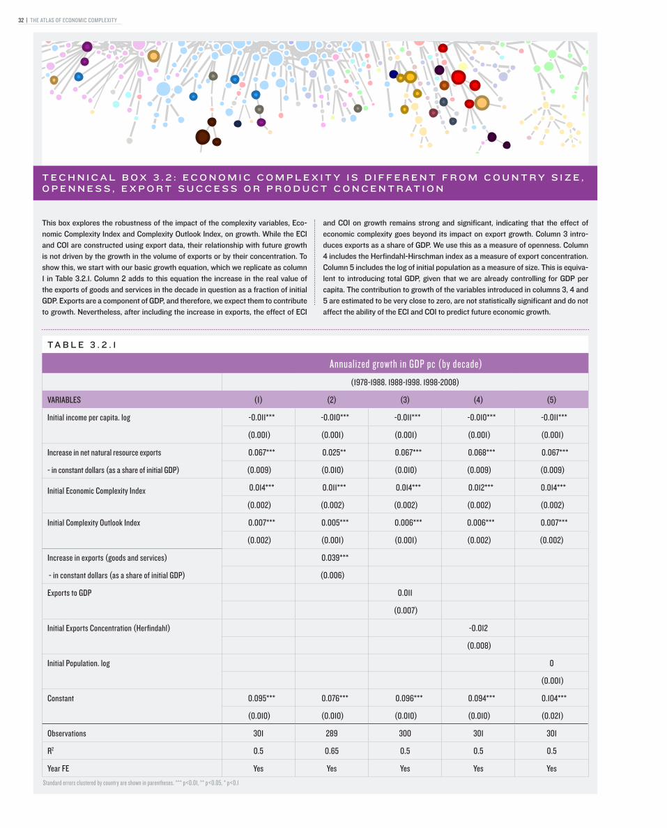
T E C H N I C A L B O X 3 . 2 : E C O N O M I C C O M P L E X I T Y I S D I F F E R E N T F R O M C O U N T R Y S I Z E , O P E N N E S S , E X P O R T S U C C E S S O R P R O D U C T C O N C E N T R AT I O N
This box explores the robustness of the impact of the complexity variables, Eco-nomic Complexity Index and Complexity Outlook Index, on growth. While the ECI and COI are constructed using export data, their relationship with future growth is not driven by the growth in the volume of exports or by their concentration. To show this, we start with our basic growth equation, which we replicate as column 1 in Table 3.2.1. Column 2 adds to this equation the increase in the real value of the exports of goods and services in the decade in question as a fraction of initial GDP. Exports are a component of GDP, and therefore, we expect them to contribute to growth. Nevertheless, after including the increase in exports, the effect of ECI
and COI on growth remains strong and significant, indicating that the effect of economic complexity goes beyond its impact on export growth. Column 3 intro-duces exports as a share of GDP. We use this as a measure of openness. Column 4 includes the Herfindahl-Hirschman index as a measure of export concentration. Column 5 includes the log of initial population as a measure of size. This is equiva-lent to introducing total GDP, given that we are already controlling for GDP per capita. The contribution to growth of the variables introduced in columns 3, 4 and 5 are estimated to be very close to zero, are not statistically significant and do not affect the ability of the ECI and COI to predict future economic growth.
T A B L E 3 . 2 . 1
Annualized growth in GDP pc (by decade)
(1978-1988. 1988-1998. 1998-2008)
VARIABLES (1) (2) (3) (4) (5)
Initial income per capita. log -0.011*** -0.010*** -0.011*** -0.010*** -0.011***
(0.001) (0.001) (0.001) (0.001) (0.001)
Increase in net natural resource exports 0.067*** 0.025** 0.067*** 0.068*** 0.067***
- in constant dollars (as a share of initial GDP) (0.009) (0.010) (0.010) (0.009) (0.009)
Initial Economic Complexity Index
0.014*** 0.011*** 0.014*** 0.012*** 0.014***
(0.002) (0.002) (0.002) (0.002) (0.002)
Initial Complexity Outlook Index 0.007*** 0.005*** 0.006*** 0.006*** 0.007***
(0.002) (0.001) (0.001) (0.002) (0.002)
Increase in exports (goods and services) 0.039***
- in constant dollars (as a share of initial GDP) (0.006)
Exports to GDP 0.011
(0.007)
Initial Exports Concentration (Herfindahl) -0.012
(0.008)
Initial Population. log 0
(0.001)
Constant 0.095*** 0.076*** 0.096*** 0.094*** 0.104***
(0.010) (0.010) (0.010) (0.010) (0.021)
Observations 301 289 300 301 301
R2 0.5 0.65 0.5 0.5 0.5
Year FE Yes Yes Yes Yes Yes
Standard errors clustered by country are shown in parentheses. *** p<0.01, ** p<0.05, * p<0.1

MAPPING PATHS TO PROSPERITY | 33
T E C H N I C A L B O X 3 . 3 : W H AT A B O U T S E R V I C E S ?
The measures, ranking and figures in this Atlas are all based on trade data, which only contains information on tradable goods. Economies, however, produce not only goods, but also services, such as tourism, finance and consulting. The lack of ser-vice data can bias our results if the complexity of a country’s service structure car-ries different information than can be inferred from its trade in goods. Yet, we can expect service data to provide little additional information in a world where coun-tries that have complex goods structures also have complex service structures.
Unfortunately, highly disaggregated data on services is not available, since services are not controlled at borders through customs agents in the way goods are. Hence, because of data constraints, we are limited to exploring the role of services at a more aggregate level. We used the service data from the World Bank based on IMF Balance of Payments dataset, which classifies ex-ports of services in 12 different categories. These categories are very broad. For instance, the transportation services category encompasses all different types of transformation such as sea, rail, air and land transportation as well as bulk, containerized and refrigerated services. Business services puts together
T A B L E 3 . 3 . 1
Annualized growth in GDPpc (by decade)
(1988-1998, 1998-2008)
VARIABLES (1) (2) (3) (4) (5) (6)
Initial income per capita, log -0.002*** -0.011*** -0.010*** -0.002*** -0.011*** -0.011***
(0.001) (0.001) (0.001) (0.001) (0.002) (0.001)
Increase in natural resource exports- in constant dollars (as a share of initial GDP)
0.055*** 0.062*** 0.062*** 0.055*** 0.062*** 0.062***
(0.013) (0.009) (0.010) (0.013) (0.009) (0.009)
Initial Economic Complexity Index (using goods) 0.016*** 0.019*** 0.016***
(0.002) (0.007) (0.002)
Initial Economic Complexity Index (using goods and services) 0.015*** -0.003
(0.002) (0.007)
Initial Economic Complexity Index (using services) -0.001 -0.001
(0.001) (0.001)
Constant 0.046*** 0.110*** 0.109*** 0.046*** 0.110*** 0.111***
(0.007) (0.012) (0.012) (0.007) (0.012) (0.012)
Observations 218 218 218 218 218 218
Adjusted R2 0.307 0.460 0.446 0.308 0.461 0.462
Year FE Yes Yes Yes Yes Yes Yes
accounting, engineering, legal and management consulting in the same category. Nevertheless, this dataset is the most diverse that we have found, so we decided to use it to see whether our results are affected by the absence of this data.
Figure 3.3.1 shows the comparison of ECIs calculated using only goods to the ECI calculated with goods and services, combined. Overall, we see an almost perfect correlation, meaning that the inclusion of services does not change our basic story. Another way of calculating ECI would be to use just the services data. We checked whether all these three indices, namely ECI calculated with goods (ECIg), ECI calcu-lated with goods and services (ECIgs) and ECI calculated only using the data from services (ECIs), are predictive of growth. Table 3.3.1 shows that ECIg and ECIgs are both good predictors of growth, whereas ECIs does not predict growth. When put together, ECIg beats ECIgs in terms of its correlation with future growth. This may be due to the fact that the services data is very coarse and does not capture well the very large differences in complexity of the different services it groups under the same heading. Hence, for now, we think that the services data is not disaggregate enough to be included in our economic complexity calculations.
Standard errors clustered by country are shown in parentheses. *** p<0.01, ** p<0.05, * p<0.1
Relationship between ECI calculated with goods and ECI calculated with goods and services.
F I G U R E 3 . 3 . 1 :
AGO
ALB
ARE
ARG
AUS
AUT
AZE
BEL
BGD
BGR
BIH
BLR
BOL
BRABWA
CAN
CHE
CHL
CHN
CIV
CMR COG
COL CRI
CUB
CZE
DEU
DNK
DOMDZAECU EGY
ESPEST
ETH
FINFRA
GAB
GBR
GEO
GHA
GIN
GRCGTM
HKG
HND
HRV
HUN
IDNIND
IRL
IRN
ISR ITA
JAM
JOR
JPN
KAZ
KENKGZ
KHM
KOR
KWT
LAO
LBN
LBR
LBY
LKA
LTU
LVA
MAR
MDA
MDG
MEX
MKD
MLI
MNGMOZ
MRT
MUSMWI
MYS
NAM
NGA
NIC
NLD
NOR
NZL
OMN
PAK
PANPERPHL
PNG
POL
PRT
PRY
QAT
ROM
RUS
SAU
SDN
SEN
SGP
SLV
SRB
SVKSVN
SWE
SYR
THA
TJKTKM
TTO TUN
TUR
TZA
UGA
UKR
URY
USA
UZBVEN VNM
YEM
ZAF
ZMB
ZWE
−2−1
01
2EC
I (go
ods a
nd se
rvice
s)
−2 −1 0 1 2
ECI (goods)

How Is Complexity Different from Other Approaches?
S E C T I O N 4

MAPPING PATHS TO PROSPERITY | 35
e are certainly not the first to look for correlates or causal factors of income and growth. One strand of the lit-erature has looked at the salience of institutions in determining growth, whereas others have looked at hu-man capital or broader measures of competitiveness. Clearly, more com-plex economies tend to have better
institutions, more educated workers and more competitive environments, so these approaches are not completely at odds with each other or with ours. In fact, the strength of institutions, quality of education, competitiveness, financial depth and economic complexity all emphasize different as-pects of the same intricate reality. It is not clear, however, that these different approaches have the same ability to capture factors that are verifiably important for growth and development. In this section, we compare each of these mea-sures with our Complexity Indices and gauge their marginal contribution to income and economic growth.
MEASURES OF GOVERNANCE AND INSTITUTIONAL QUALITYSome of the most respected measures of institutional qual-ity are the six Worldwide Governance Indicators (WGIs), which the World Bank has published biennially since 1996. These indicators are used, for example, as eligibility crite-ria by the Millennium Challenge Corporation (MCC) to se-lect the countries they choose to support. These criteria are based on the presumption of a causal connection between governance, on the one hand, and potential for growth and poverty reduction, on the other.
WTo the extent that governance is important to allow in-
dividuals and organizations to cooperate, share knowledge and make more complex products, it should be reflected in the kind of industries that a country can support. There-fore, the Economic Complexity variables indirectly capture information about the quality of governance in a country. Which indicator captures information that is more relevant for growth is an empirical question.
Here we compare the contribution to the predictibality of future economic growth accounted for by the WGIs and the Economic Complexity variables, ECI and COI using a tech-nique described in Technical Box 4.1. Briefly, our technique involves removing the variables of interest, either one by one or in groups, from an estimation equation that initially in-cludes all of the variables. This allows us to determine how much of the predictive power can be attributed singularly to each variable. The attributions are measured as the amount of variance that is accounted uniquely by the variable of in-terest. Since the WGIs are available only since 1996, we per-form this exercise using the 1996-2008 period as a whole and as two consecutive 6-year periods. We also compare with each individual WGI and with the six of them together.
Figure 4.1 shows that the Economic Complexity vari-ables account for 18.3 percent of the variance in economic growth during the 1996-2008 period, while the six WGIs combined account only for 3 percent. For the estimation using the two six-year periods, we find that ECI accounts for 10.9% of the variance in growth, whereas the six WGIs combined account for 2.2%.
We conclude that as far as future economic growth is con-cerned, the Economic Complexity and Complexity Outlook

36 | THE ATLAS OF ECONOMIC COMPLEXITY
Indices capture significantly more growth-relevant infor-mation than the 6 World Governance Indicators, either individually or combined. This does not mean that gover-nance is not important for the economy. It suggests that the aspects of governance important for growth are weakly re-flected in the WGIs and appear to be more strongly reflected in measures of economic complexity.
EDUCATION-BASED MEASURES OF HUMAN CAPITALAnother strand of the growth and development literature has looked at the impact of human capital on economic growth. The idea that human capital is important for income and growth is not unrelated to our focus on the productive knowledge that exists in a society. The human capital lit-erature, however, has placed its attention on the amount of knowledge the average citizen has, and has measured this in years of formal education. Our approach emphasizes the variety of productive knowledge that different individuals have, including their tacit knowledge, and emphasizes the interactions that enable productive knowledge to be used in networks of individuals and firms.
The standard variables used as a proxy for human capi-tal are the number of years of formal schooling attained by those currently of working age, as well as the school enroll-ment rates of the young population (Barro and Lee, 2010). Since these indicators do not take into account the quality of the education received by pupils, they have been subject to criticism resulting in new measures of educational quality. These measures use test scores from standardized interna-tional exams, such as the OECD Programme for Internation-al Student Assessment (PISA) or the Trend in International
Contribution to the variance of economic growth from complexity variables (ECI and COI) and from the measures of governance and institutional quality.
F I G U R E 4 . 1 :
Mathematics and Science Study (TIMSS). Hanuschek and Woessmann (2008) collected data for all the countries that participated in either program and used this information to generate a measure of the average cognitive ability of stu-dents for a cross-section of countries around the year 2000.
The information about productive knowhow captured by the economic complexity variables, and the information re-flected in education-based measures of human capital are not just two sides of the same coin. Analytically, education indicators try to measure how much of the same knowledge individuals have, whether knowledge is measured as years of study of the national curriculum or as the skills mastered by students according to standardized international tests. In contrast, the Economic Complexity variables try to capture the total amount of productive knowledge that is embed-ded in a society as a whole and is related to the diversity of knowledge that its individuals have. Clearly, for a complex economy to exist, its members must be able to read, write and manipulate symbols, such as numbers or mathematical functions. This is what is taught in schools. Yet, the converse is not true: the skills acquired in school may be a poor proxy for the productive knowledge of a society.
What a society can produce, however, often has little re-lationship to what people learn in school. For example, if a country were to achieve the goal of having every pupil complete a good secondary education and if this was the extent of its productive knowledge, no one would know how to make a pair of shoes, a metal knife, a roll of paper or a patterned piece of cotton fabric. The skills that are required to make these products are acquired mostly on the job. That is why job advertisements often request years of particular
0% 4% 8% 12% 16% 20.0%
Regulatory Quality
Rule of Law
Control of Corruption
Government Effectiveness
Voice and Accountability
Political Stability
All institutional variables
Economic Complexity Variables
12 years
6 years

MAPPING PATHS TO PROSPERITY | 37
experience, not just years of schooling. In fact, what a coun-try produces determines the kinds of skills its citizens can acquire through on-the-job experience. The education-based human capital approach overlooks this important fact by assuming implicitly that what workers formally study is what affects what a society is able to do.
Figure 4.2 shows the relationship between our measure of economic complexity and years of schooling for the year 2000. It is clear that there is positive relationship between the two (R2=50%). Countries like India and Uganda, or Mon-golia and Mexico, have very similar levels of average formal education. Yet, they differ dramatically in economic com-plexity. India is much more complex than Uganda, and Mex-ico is much more complex than Mongolia.
Figure 4.3 shows that the relationship between cognitive ability and economic complexity is also positive. Here we find that Brazil and Ghana are two countries with similar lev-els of cognitive ability, but very different levels of economic complexity. Brazil is two standard deviations more complex than Ghana. The same is true for Colombia and Nigeria. Their measured cognitive abilities are the same, but Colombia is nearly 1.5 standard deviations more complex than Nigeria.
For illustration purposes, consider the case of Ghana and Thailand. Both countries had similar levels of schooling in 1970, but Ghana expanded education more vigorously than Thailand in the subsequent 40 years (Figure 4.4). However, Ghana’s economic complexity and income stagnated as it remained an exporter of cocoa, aluminum, fish and forest products. By contrast, between 1970 and 1985 Thailand un-derwent a massive increase in economic complexity, equiv-alent to a change of one standard deviation in the Economic
Complexity Index (Figure 4.5). This caused a sustained eco-nomic boom in Thailand after 1985. As a consequence, the level of income per capita between Ghana and Thailand has since diverged dramatically (Figure 4.6). Ghana’s population may have gone through more schooling than Thailand’s, but Thailand has more productive knowledge.
Next, we measure how well these indicators account for the current level of income of countries and to predict future eco-nomic growth, using the same technique that we employed to compare Economic Complexity variables, ECI and COI, with the World Governance Indicators (see Technical Box 4.1). We begin by looking at the level of income per capita. While data on years of schooling and school enrollment is available for several years, the data on educational quality exists only for a cross-section of countries around the year 2000. We use the data for this year to estimate equations where the dependent variable is the level of income per capita and the independent variables are the years of schooling of the labor force, the Ha-nushek and Woessmann measure of cognitive ability, and the ECI. We do not use school enrollment as this variable affects future human capital but not the human capital invested in creating today’s income. The results, presented in Figure 4.7, indicate that the Economic Complexity Index explains 17 percent of the variance, after controlling for the education variables, while years of schooling and cognitive ability to-gether account for only 4 percent of the variance that is not explained by the complexity variables. This shows that the ECI contains more information relevant to the generation of income than the educational variables.
We also look at how well human capital and complexity explain future growth. To do this we follow a methodology
ALB
ARE
ARG AUS
AUTBEL
BGD
BGR
BOL
BRA
CAN
CHE
CHL
CHN
CIV
CMR
COG
COL
CRI
CUB
CZE
DEU
DNK
DZA
ECU
EGY
ESP
EST
FIN
FRA
GAB
GBR
GHA
GRC
GTM
HKG
HND
HRV
HUN
IDN
IND
IRL
IRN
ISR
ITA
JAM
JOR
JPN
KAZ
KEN
KGZ
KHM
KOR
KWT
LAO
LBRLBY
LKA
LTULVA
MAR
MEX
MLIMNG
MOZ
MRT
MUS
MWI
MYS
NIC
NLD
NOR
NZL
PAK
PANPER
PHL
PNG
POL
PRT
PRYQAT
ROM
RUS
SAU
SDN
SEN
SGP
SLV
SVKSVN
SWE
SYR
THA
TJK
TTO
TUN
TUR
TZAUGA
UKR
URY
USA
VEN
VNM
YEM
ZAF
ZMB
ZWE
−2−1
01
23
Econ
omic
Comp
lexity
Inde
x
0 5 10 15
Years of schooling
ALB
ARG AUS
AUT
BEL
BGR
BRA
CAN
CHE
CHL
CHN
COL
CZEDNK
EGY
ESP
EST
FINFRA
GBR
GHA
GRC
HKG
HUN
IDN
IND
IRL
IRN
ISR
ITA
JOR
JPN
KOR
KWTLBN
LTU LVA
MAR
MDA
MEX
MKD
MYS
NGA
NLD
NOR
NZL
PER
PHL
POL
PRTROM
RUS
SAU
SGPSVK
SVN
SWE
THA
TUN
TUR URY
USA
ZAF
ZWE
−2−1
01
23
Econ
omic
Comp
lexity
Inde
x
3 3.5 4 4.5 5 5.5
Cognitive Ability
Relationship between Years of Schooling and the Economic Complexity Index (ECI) for the year 2000.
F I G U R E 4 . 2 :
Relationship between Cognitive Ability and the Economic Complexity Index (ECI) for the year 2000.
F I G U R E 4 . 3 :
Years of Schooling Cognitive Ability
Econ
omic
Com
plex
ity In
dex
Econ
omic
Com
plex
ity In
dex

38 | THE ATLAS OF ECONOMIC COMPLEXITY
similar to that used for the analysis of governance on growth (see Technical Box 4.2). In this case, we include data on school enrollment at the secondary and tertiary levels as these would affect the years of schooling of the labor force going forward. We do not include cognitive ability as this variable exists only for a single year.
Figure 4.8 shows that economic complexity accounts for 15 percent of the variance in economic growth rates unex-plained by education for the three decades between 1978 and 2008. All education variables, on the other hand, when combined account only for 3 percent of the variance not ex-plained by economic complexity.
These results show that the Economic Complexity Index contains information that is more directly related to a coun-try’s level of income and its future rate of growth than the standard variables used to measure human capital.
MEASURES OF COMPETITIVENESSLet us now turn to measures of competitiveness. The most respected source of these measures is the World Economic Forum’s Global Competitiveness Index (GCI). The GCI has been published since 1979. Over the course of more than 30 years, the coverage of the GCI has been expanded and im-proved methodologically, going through two major revisions in 2001 and 2006. In 1995, the Global Competitiveness Re-port (GCR) ranked less than 50 countries, but over the years this number has increased and now it ranks over 130 coun-tries. The claim of the GCR is that the GCI captures the fun-damental variables that drive growth in the medium term:
“We define competitiveness as the set of institutions, policies, and factors that determine the level of productivity of a country. Because the rates of return are the fundamental
drivers of the growth rates of the economy, a more competitive economy is one that is likely to grow faster
in the medium to long run.” (global competitiveness report 2010 chapter 1.1, page 4)
2.000
04.0
000
6.000
08.0
000
Year
s of S
choo
ling
1960 1970 1980 1990 2000 2010year
Ghana Thailand
−6−4
−20
2
1960 1970 1980 1990 2000 2010
010
0020
0030
00
GDP p
er ca
pita (
cons
tant 2
000 U
S$)
1960 1970 1980 1990 2000 2010year
Ghana Thailand
Years of schooling of Thailand and Ghana as a function of time.
F I G U R E 4 . 4 :
Economic Complexity Index (ECI) of Thailand and Ghana as a function of time.
F I G U R E 4 . 5 :
Evolution of the GDP per capita of Thailand and Ghana as a function of time.
F I G U R E 4 . 6 :
Year
of S
choo
ling
Econ
omic
Com
plex
ity In
dex
GDP
per c
apita
(con
stan
t 200
0 US
$)

MAPPING PATHS TO PROSPERITY | 39
Contribution to the variance of income from the Economic Complexity Index (ECI) and measures of human capital from Hanuschek and Woessmann (2008).
F I G U R E 4 . 7 :
Contribution to the variance of economic growth from the Economic Complexity Index (ECI) and measures of human capital from Barro and Lee (2010).
F I G U R E 4 . 8 :
0% 3% 6% 9% 12% 15% 18%
Cognitive Abilities
Years of Schooling
All Education Variables
Economic Complexity
0% 4% 8% 12% 16%
Secondary School Enrollment
Tertiary School Enrollment
Years of Schooling
All Education Variables
Economic Complexity Variables

40 | THE ATLAS OF ECONOMIC COMPLEXITY
The GCR develops over 150 measures of elements that it considers important for competitiveness and then aver-ages them. The ECI looks, instead, at the actual industries that a country can support. Both should capture informa-tion that is relevant to an economy’s ability to grow. Next, we compare the two rankings to establish which captures more growth-relevant informations.
Since we only have data for the GCI rankings, and not the underlying values of the index, we do the analysis using the rankings of the Economic Complexity Index. This allows for a fairer comparison. We compare using 5- and 10-year pan-els starting in 1979. What we find is surprising: with 10-year panels, the complexity variables explain 15 percent more of the variance unexplained by the GCI, while the GCI ex-plains only 1 percent of the variance not explained by the ECI. This means that the GCI rankings are less informative about growth prospects than the complexity indicators (see Technical Box 4.3 and Figure 4.9).
MEASURES OF FINANCIAL DEPTHThere is a broad literature discussing the links between fi-nance and growth. How much the financial sector lends rela-tive to the size of the economy is referred to as the ‘depth’ of the financial system, and there are varying interpretations of the role this plays in growth. Some have found a posi-tive effect (King and Levine, 1993; Beck, Levine and Loayza, 2000; Demirgüç-Kunt and Levine, 2001; Levine, 2005; Aghion, Howitt, and Mayer-Foulkes, 2005), while others have found inconclusive (Easterly, 2005; Trew, 2006) or even negative links (Arcand, Berkes and Panizza, 2012).
The typical argument in favor of a connection between
finance and growth is the following: when a financial sys-tem is able to discriminate between good and bad invest-ments, more people will be willing to trust the system with their savings. Entrepreneurs with good projects but little capital will be more able to implement their ideas, which would in turn lead to higher growth. Development of the financial sector has been seen as critical to overall develop-ment strategies in recent decades, and has received priority attention from the World Bank, the International Monetary Fund and other development agencies.
Here we contrast how strongly standard financial depth indicators and complexity indicators correlate with subse-quent growth. For measures of financial depth we use the two most frequently used financial variables in this area, the ratio to GDP of domestic credit provided by the banking system, either in total or restricted to the private sector. We use both measures because, as argued by Barro and Sala-i-Martin (2004), financing greater government con-sumption may not contribute to growth as much as other forms of private spending.
To study the relative importance of complexity in-dicators and financial depth indicators on growth, we apply the same method we have been using through-out this chapter. Figure 4.10 and Technical Box 4.4 pres-ent our results. For the three decades starting in 1978, the economic complexity variables can account for 21.5 percent of the variance in 10-year growth rates that is unexplained by the financial development vari-ables, the initial level of development, and the growth in natural resource income. This represents an increase of more than 74 percent in future growth predictability
Contribution to the variance of economic growth from the Economic Complexity Index (ECI) and measures of competitiveness.
F I G U R E 4 . 9 :
0% 2% 4% 6% 8% 10% 12% 14% 16% 18%
5 Years
10 Years Economic Complexity Ranking
WEF - Competitiveness Ranking

MAPPING PATHS TO PROSPERITY | 41
relative to the equation that excludes the complexity variables. By contrast, after controlling for the complex-ity indicators, the level of development and the growth in natural resource exports, the measures of financial depth are not statistically or economically significant and con-tribute essentially nothing to the predictability of future growth, whether taken individually or jointly. We conclude that complexity indicators hold more growth-relevant in-formation relative to measures of financial depth. A view including financial measures does not offer more statisti-cally significant insights than complexity taken on its own.
EXPORT SOPHISTICATION MEASURESIn 2007 Hausmann, Hwang and Rodrik (HHR) developed a measure of product and country sophistication using export data and showed that it was correlated with future growth: countries converged to the income level of their competitors in export markets. The HHR paper, by using export data and by using information on other countries to characterize a given country, inspired our approach. However the variables HHR developed are different. To measure complexity of a product, which they called PRODY, they calculate average wealth of the countries that export this product. PRODY is the weighted average of the GDP per capita of the countries that export the product, where the weights are given by the Revealed Comparative Advantage (RCA, see Technical Box 2.2) of the country in that product. They then calculate the export sophistication of a country, which they call EXPY. This variable can be interpreted as a measure of how rich a country’s competitors are, meaning how rich, on average, is a synthetic combination of countries that export the same
basket of goods that a particular country exports. This is cal-culated as the weighted average of the PRODYs where the weights are the shares of each product in the country’s ex-port basket (see Technical Box 4.5).
The major difference between our approach and HHR is that EXPY uses information about the GDP per capita of countries that export the same products as a particular country, while ECI and COI do not use GDP per capita infor-mation. Instead, ECI and COI exploit the network of connec-tions between a country, the products that it makes, the oth-er countries that make them, the products that they make, etc. This is a cleaner measure, as we do not use information on GDP per capita of other countries to explain either the GDP per capita or the growth rate of a given country. But does it perform better in explaining growth?
We compared EXPY with ECI in predicting growth (see Technical Box 4.5) and conclude that, while EXPY does correlate with future growth, it explains a smaller frac-tion of the variance of growth, and when put together with ECI, the contribution of EXPY becomes statistically insignificant, while the effect of ECI remains fundamen-tally unaffected.
Overall, we are able to conclude that the Economic Com-plexity variables contain more information regarding the income and growth potential of countries than other com-monly used indicators. Considered alongside measures of governance, human capital, competitiveness or even country and product sophistication, Economic Complexity measures are best able to predict future growth.
Contribution to the variance of economic growth from the Economic Complexity variables (ECI and COI) and measures of financial depth.
F I G U R E 4 . 1 0 :
0% 5% 10% 15% 20% 25%
Domestic credit to private sector (% of GDP)
Domestic credit provided by banking sector (% of GDP)
All finance variables
Economic Complexity variables

42 | THE ATLAS OF ECONOMIC COMPLEXITY
T E C H N I C A L B O X 4 . 1 : G O V E R N A N C E A N D C O M P L E X I T Y
We compare the contribution to economic growth of the Worldwide Gover-nance Indicators (WGIs) and economic complexity by estimating a growth regression where all of the WGIs and the Economic Complexity variables are used as explanatory variables. As controls we include the logarithm of per
T A B L E 4 . 1 . 1
Annualized growth in GDP pc
1996-2002, 2002-2008
VARIABLES (1) (2) (3) (4) (5) (6) (7) (8) (9)
Initial income per capita, log -0.00268*** -0.00158*** -0.00267*** -0.00270*** -0.00270*** -0.00264*** -0.00270*** -0.00266*** -0.00236***
(0.000) (0.000) (0.000) (0.000) (0.000) (0.000) (0.000) (0.000) (0.000)
Net natural resource exports as a share of GDP 0.01618*** 0.01139*** 0.01616*** 0.01624*** 0.01598*** 0.01624*** 0.01633*** 0.01623*** 0.01568***
(0.003) (0.004) (0.003) (0.003) (0.003) (0.003) (0.003) (0.003) (0.003)
Increase in net natural resource exports 0.00119 -0.00239 0.00114 0.00128 0.00119 0.00126 0.00125 0.00133 0.00095
- in constant dollars (as a share of initial GDP) (0.004) (0.004) (0.004) (0.004) (0.003) (0.003) (0.003) (0.003) (0.003)
Initial Economic Complexity Index 0.00262*** 0.00271*** 0.00258*** 0.00271*** 0.00264*** 0.00266*** 0.00259*** 0.00274***
(0.001) (0.001) (0.001) (0.001) (0.001) (0.001) (0.001) (0.001)
Initial Complexity Outlook Index 0.00076*** 0.00075*** 0.00076*** 0.00067** 0.00078*** 0.00074*** 0.00075*** 0.00069**
(0.000) (0.000) (0.000) (0.000) (0.000) (0.000) (0.000) (0.000)
Initial Control of Corruption -0.00004 -0.00121 -0.00020 -0.00012 0.00014 -0.00004 -0.00006
(0.001) (0.001) (0.001) (0.001) (0.001) (0.001) (0.001)
Initial Government Effectiveness -0.00040 0.00096 -0.00069 -0.00026 -0.00022 -0.00044 -0.00040
(0.001) (0.001) (0.001) (0.001) (0.001) (0.001) (0.001)
Initial Political Stability 0.00102** 0.00097** 0.00090* 0.00100** 0.00111** 0.00102** 0.00098**
(0.000) (0.000) (0.000) (0.000) (0.000) (0.000) (0.000)
Initial Rule of Law 0.00061 0.00142 0.00083 0.00048 0.00126 0.00056 0.00055
(0.001) (0.001) (0.001) (0.001) (0.001) (0.001) (0.001)
Initial Regulatory Quality -0.00017 -0.00114 -0.00012 -0.00021 -0.00024 -0.00009 -0.00032
(0.001) (0.001) (0.001) (0.001) (0.001) (0.001) (0.001)
Initial Voice and Accountability -0.00028 0.00023 -0.00027 -0.00028 -0.00012 -0.00025 -0.00034
(0.001) (0.001) (0.001) (0.001) (0.001) (0.001) (0.001)
Constant 0.02505*** 0.01706*** 0.02503*** 0.02516*** 0.02517*** 0.02473*** 0.02521*** 0.02491*** 0.02252***
(0.003) (0.003) (0.003) (0.003) (0.003) (0.003) (0.003) (0.003) (0.003)
Observations 243 243 244 243 243 243 243 243 248
R2 0.568 0.459 0.566 0.568 0.558 0.568 0.568 0.568 0.546
R2 difference 10,9% 0,2% 0,0% 1,0% 0,0% 0,0% 0,0% 2,2%
Year FE Yes Yes Yes Yes Yes Yes Yes Yes Yes
capita income, the increase in natural resource exports during the period and the initial share of GDP represented by natural resource exports. The contribution of each variable is estimated by taking the difference between the R2 obtained for the regression using all variables and that obtained for
Robust standard errors in parentheses *** p<0.01, ** p<0.05, * p<0.1

MAPPING PATHS TO PROSPERITY | 43
the regression where the variable was removed.Table 4.1.1 shows the results of this procedure using two consecutive six-
year periods. Table 4.1.2 shows the same procedure using one twelve-year pe-riod (1996-2008). Figure 4.1 of the main text, illustrates the differences in R2
T A B L E 4 . 1 . 2
Annualized growth in GDP pc (12 years)
1996-2008
VARIABLES (1) (2) (3) (4) (5) (6) (7) (8) (9)
Initial income per capita, log -0.00223*** -0.00160*** -0.00221*** -0.00231*** -0.00225*** -0.00216*** -0.00221*** -0.00218*** -0.00212***
(0.000) (0.000) (0.000) (0.000) (0.000) (0.000) (0.000) (0.000) (0.000)
Net natural resource exports as a share of GDP 0.00807*** 0.00647*** 0.00802*** 0.00811*** 0.00780*** 0.00810*** 0.00799*** 0.00798*** 0.00783***
(0.001) (0.002) (0.001) (0.001) (0.001) (0.001) (0.001) (0.001) (0.001)
Increase in net natural resource exports 0.00438*** 0.00366* 0.00427*** 0.00457*** 0.00433*** 0.00439*** 0.00435*** 0.00460*** 0.00448***
- in constant dollars (as a share of initial GDP) (0.001) (0.002) (0.001) (0.001) (0.001) (0.001) (0.001) (0.001) (0.001)
Initial Economic Complexity Index 0.00237*** 0.00243*** 0.00223*** 0.00247*** 0.00241*** 0.00234*** 0.00227*** 0.00235***
(0.000) (0.000) (0.000) (0.000) (0.000) (0.000) (0.000) (0.000)
Initial Complexity Outlook Index 0.00066** 0.00062** 0.00069*** 0.00058** 0.00069*** 0.00067*** 0.00065** 0.00065***
(0.000) (0.000) (0.000) (0.000) (0.000) (0.000) (0.000) (0.000)
Initial Control of Corruption 0.00030 -0.00074 -0.00009 0.00024 0.00046 0.00030 0.00008
(0.001) (0.001) (0.001) (0.001) (0.001) (0.001) (0.001)
Initial Government Effectiveness -0.00091 0.00007 -0.00091 -0.00077 -0.00075 -0.00090 -0.00073
(0.001) (0.001) (0.001) (0.001) (0.001) (0.001) (0.001)
Initial Political Stability 0.00072** 0.00074 0.00060 0.00066* 0.00082** 0.00071** 0.00060*
(0.000) (0.000) (0.000) (0.000) (0.000) (0.000) (0.000)
Initial Rule of Law 0.00064 0.00199** 0.00093 0.00038 0.00102 0.00067 0.00049
(0.001) (0.001) (0.001) (0.001) (0.001) (0.001) (0.001)
Initial Regulatory Quality 0.00010 -0.00085 0.00012 0.00002 0.00002 0.00019 -0.00022
(0.001) (0.001) (0.001) (0.001) (0.001) (0.001) (0.001)
Initial Voice and Accountability -0.00070 -0.00016 -0.00064 -0.00061 -0.00056 -0.00065 -0.00067
(0.000) (0.001) (0.000) (0.000) (0.000) (0.000) (0.000)
Constant 0.02068*** 0.01605*** 0.02055*** 0.02123*** 0.02073*** 0.02019*** 0.02057*** 0.02034*** 0.01969***
(0.002) (0.003) (0.002) (0.002) (0.002) (0.002) (0.002) (0.002) (0.002)
Observations 119 119 120 119 119 119 119 119 122
R2 0.618 0.435 0.613 0.613 0.609 0.616 0.618 0.610 0.588
R2 difference 18,3% 0,5% 0,5% 0,9% 0,2% 0,0% 0,8% 3,0%
Robust standard errors in parentheses *** p<0.01, ** p<0.05, * p<0.1
between the regression using all variables and those where individual vari-ables were removed.

44 | THE ATLAS OF ECONOMIC COMPLEXITY
T E C H N I C A L B O X 4 . 2 : E D U C AT I O N , C O G N I T I V E A B I L I T Y A N D E C O N O M I C C O M P L E X I T Y
We compare the contribution to income of education, cognitive ability and eco-nomic complexity by regressing income against years of schooling, cognitive ability and the Economic Complexity Index. The contribution to income of each variable is estimated by taking the difference between the R2 obtained for the regression using all variables and that obtained for a regression where the vari-able in question was removed.
Table 4.2.1 shows the results of this procedure for the year 2000, when cog-nitive ability data is available. Figure 4.7 in the main text summarizes the results.
We compare the contribution to growth of education and economic
complexity variables by regressing growth against years of schooling secondary school enrollment, tertiary school enrollment, the Economic Complexity Index and the Complexity Outlook Index. As additional controls we include the change in natural resource exports during the period, the logarithm of per capita income and year fixed effects. The contribution of each variable to growth is estimated by taking the difference between the R2 obtained for a regression using all variables and one obtained for a regression where the variable in question was removed.
Table 4.2.2 shows the results of this procedure for ten year panels start-ing in 1978, 1988 and 1998. Figure 4.8 in the main text summarize the results.
T A B L E 4 . 2 . 1
Income per capita, log – Year 2000
VARIABLES (1) (2) (3) (4) (5)
Economic Complexity Index 1.013*** 1.085*** 1.024*** 1.245***
(0.182) (0.194) (0.143) (0.114)
Years of schooling 0.148* 0.209** 0.151**
(0.081) (0.086) (0.073)
Cognitive ability 0.027 0.876*** 0.287
(0.279) (0.290) (0.275)
Constant 6.585*** 2.884*** 6.645*** 6.675*** 7.844***
(1.043) (0.997) (1.114) (0.606) (0.167)
Observations 60 60 60 60 60
R2 0.598 0.432 0.569 0.598 0.561
Difference in R2 0.17 0.03 0.00 0.04
Robust standard errors in parentheses *** p<0.01, ** p<0.05, * p<0.1

MAPPING PATHS TO PROSPERITY | 45
T A B L E 4 . 2 . 2
Annualized growth in GDP pc (by decade)
(1978-1988, 1988-1998, 1998-2008)
VARIABLES (1) (2) (3) (4) (5) (6)
Initial Income per capita, log -0.012*** -0.006*** -0.011*** -0.012*** -0.012*** -0.010***
(0.002) (0.001) (0.001) (0.002) (0.002) (0.001)
Increase in natural resource exports 0.068*** 0.048* 0.068*** 0.069*** 0.068*** 0.075***
- in constant dollars (as a share of initial GDP) (0.025) (0.027) (0.026) (0.025) (0.025) (0.026)
Initial Economic Complexity Index 0.011*** 0.012*** 0.011*** 0.011*** 0.013***
(0.002) (0.002) (0.002) (0.002) (0.002)
Initial Complexity Outlook Index 0.006*** 0.007*** 0.006*** 0.006*** 0.007***
(0.002) (0.002) (0.002) (0.002) (0.002)
Years of schooling (standardized) 0.008* 0.013*** 0.009*** 0.004
(0.004) (0.004) (0.002) (0.003)
Secondary school enrollment (standardized) 0.001 0.002 0.005*** 0.003
(0.003) (0.003) (0.002) (0.003)
Tertiary school enrollment (standardized) -0.004* -0.004* -0.001 -0.004**
(0.002) (0.002) (0.001) (0.002)
Constant 0.117*** 0.074*** 0.111*** 0.118*** 0.119*** 0.105***
(0.013) (0.012) (0.012) (0.013) (0.013) (0.011)
Observations 275 275 275 275 275 275
R2 0.412 0.264 0.402 0.412 0.405 0.378
Year FE Yes Yes Yes Yes Yes Yes
Difference in R2 0.15 0.01 0.00 0.01 0.03
Robust standard errors in parentheses *** p<0.01, ** p<0.05, * p<0.1

46 | THE ATLAS OF ECONOMIC COMPLEXITY
T E C H N I C A L B O X 4 . 3 : G L O B A L C O M P E T I T I V E N E S S I N D E X A N D G R O W T H
T A B L E 4 . 3 . 1
Annualized growth in GDP pc (by decade)
5 year panels 10 year panels
VARIABLES (1) (2) (3) (4) (5) (6)
Ranking of GCI -0.00054** -0.00032 -0.00025 -0.00005
(0.000) (0.000) (0.000) (0.000)
Ranking of ECI -0.00064*** -0.00052*** -0.00057*** -0.00052***
(0.000) (0.000) 0 (0.000)
Initial income per capita, logs -0.01562*** -0.00490*** -0.01152*** -0.01388*** -0.00463** -0.01183***
(0.004) (0.002) (0.003) (0.004) (0.002) (0.003)
Increase in natural resource exports 0.03144 -0.03117 0.01553 0.07837* 0.02263 0.07271*
- in constant dollars (as a share of initial GDP) (0.058) (0.058) (0.059) (0.042) (0.040) (0.039)
Constant 0.19376*** 0.07390*** 0.13923*** 0.17354*** 0.06911*** 0.14689***
(0.046) (0.017) (0.033) (0.041) (0.023) (0.030)
Observations 101 101 101 81 81 81
Adjusted R2 0.223 0.069 0.160 0.243 0.088 0.235
Year FE Yes Yes Yes Yes Yes Yes
Difference in R2 0,154 0,063 0,155 0,008
Here we compare the contribution of the Global Competitiveness Index (GCI) and the ECI to economic growth. We use the ranking of countries in the GCI and the ranking of countries in ECI to predict growth using 5 and 10 year panels. As controls, we use the increase in natural resource exports during the period as well as the logarithm of the initial GDP per capita and year fixed effects. We estimate the contribution of the GCI and ECI to growth by taking the difference
Robust standard errors in parentheses *** p<0.01, ** p<0.05, * p<0.1
between the R2 obtained for the equation in which they were both included and that in which one or the other is missing.
Table 4.3.1 shows that eliminating the rank of the ECI from the regression results in a much larger loss of explanatory power than removing the rank of GCI. This is true for both 5 and 10 year panels. Figure 4.9 on the main text illustrates these results.

MAPPING PATHS TO PROSPERITY | 47
T E C H N I C A L B O X 4 . 4 : F I N A N C I A L D E P T H
In this Technical Box we explore the impact of financial development on growth after accounting for complexity indicators and vice versa. We use data for the three 10-year periods since 1978. We measure financial depth through two vari-ables. First, we consider the ratio to GDP of total domestic credit provided by the banking system. Second, we consider the ratio to GDP of credit to the pri-vate sector provided by the banking system. We measure these variables at the start of each 10-year period. We also control for the initial level of GDP per capita and the growth of the value of natural resource exports during the period. Table 4.4.1 shows our results. The first column includes all the variables under consideration. In this regression the complexity variables remain highly signifi-cant, both economically and statistically, while the financial variables have es-sentially no relationship with growth. The overall R2 of the equation is 0.504. To
T A B L E 4 . 4 . 1
Annualized growth in GDP pc ( by decade)
(1978-1988, 1988-1998, 1998-2008)
VARIABLES (1) (2) (3) (4) (5)
Initial income per capita, log -0.01053*** -0.00166 -0.01043*** -0.01026*** -0.01066***
(0.002) (0.002) (0.002) (0.002) (0.002)
Increase in natural resource exports- in constant dollars (as a share of initial GDP)
0.07468*** 0.06949*** 0.07474*** 0.07555*** 0.07612***
(0.009) (0.010) (0.009) (0.009) (0.009)
Initial Economic Complexity Index 0.01607*** 0.01611*** 0.01572*** 0.01504***
(0.002) (0.002) (0.002) (0.002)
Initial Complexity Outlook Index 0.00650*** 0.00652*** 0.00661*** 0.00665***
(0.002) (0.002) (0.002) (0.002)
Domestic credit to private sector (% of GDP) 0.00002 0.00010 -0.00005
(0.000) (0.000) (0.000)
Domestic credit provided by banking sector (% of GDP) -0.00006 -0.00001 -0.00005
(0.000) (0.000) (0.000)
Constant 0.11082*** 0.03633** 0.11019*** 0.10780*** 0.10874***
(0.014) (0.014) (0.013) (0.013) (0.012)
Observations 277 277 277 277 277
Adjusted R2 0.504 0.287 0.505 0.503 0.503
Year FE Yes Yes Yes Yes Yes
R2 difference 0,217 0 0,001 0,001
estimate the marginal contribution of financial depth variables after controlling for complexity variables, we compare column 1 with columns 2, 3 and 4, which sequentially eliminate one, the other, and then both financial variables. In all these equations, the R2 as well as the coefficients on the complexity variables are essentially unaffected, while estimated coefficients on the remaining financial variables are essentially zero. To estimate the marginal impact of the complexity variables we compare column 1 with column 5, which excludes both complexity variables. Here the R2 declines from 0.504 to 0.215 – a 74 percent decline – while the coefficients on the financial variables remain essentially equal to zero.
We conclude that the complexity indicators are much more strongly informa-tive of subsequent growth than the financial depth indicators, whether consid-ered individually or in group.
Standard errors clustered by country are shown in parentheses. *** p<0.01, ** p<0.05, * p<0.1

48 | THE ATLAS OF ECONOMIC COMPLEXITY
T E C H N I C A L B O X 4 . 5 : E X P Y A N D E C I
In an influential paper, Hausmann, Hwang and Rodrik (HHR) showed that what a country exports – and not just how much a country exports – affects its in-come level. To characterize the degree of sophistication of a product, HHR cal-culated the average wealth of the countries that make that product and called it PRODY. To characterize the degree of sophistication of a country’s exports, they calculated the average income of a country’s competitors and called it EXPY. More precisely, product sophistication, PRODY, was obtained by taking a weighted average of the per-capita GDPs of the countries exporting the product. The weights are given by the revealed comparative advantage of each country in that product to distinguish between the successful and unsuccessful export-ers of the product. Formally, PRODY of a product is defined as:
where is the export of country c of product p. Here we do not include the country of interest in the calculation of the PRODY of its exports in order to avoid circularity. From this product level variable, HHR calculate a country-level measure EXPY, using a weighted average of the PRODY’s of a country’s exports where the weights are the export shares of the country in the product:
Relation between ECI and EXPY for year 2010 (R2 =50%)
F I G U R E 4 . 5 . 1 :
AGO
ALB
AREARG
AUS
AUT
AZE
BEL
BGD
BGRBIH
BLRBOL
BRABWA
CANCHE
CHL
CHN
CIV
CMR
COG COL
CRI
CZE
DEUDNK
DOM
DZA
ECU
EGY
ESPEST
ETH
FINFRA
GAB
GBR
GEO
GHA
GIN
GRC
GTM
HKG
HND
HRV
HUN
IDN
IND
IRL
ISR ITA
JAM
JOR
JPN
KAZ
KEN
KGZ
KHM
KOR
KWT
LAO
LBN
LBR
LKA
LTULVA
MAR
MDA
MDG
MEX
MKD
MLI
MNG
MOZ
MRT
MUS
MWI
MYS
NAM
NGA
NIC
NLD
NOR
NZL
OMN
PAK
PAN
PER
PHL
PNG
POLPRT
PRYQAT
ROMRUS
SAU
SDN
SEN
SGP
SLV
SRB
SVK
SVN SWE
SYR
THA
TJK
TKM
TTO
TUN
TUR
TZA
UGA
UKRURY
USA
UZB
VEN
VNM
YEM
ZAF
ZMB
ZWE
−3−2
−10
12
EXPY
, log
−2 −1 0 1 2
ECI
HHR showed that these variables predict GDP growth of countries. Figure 4.5.1 shows that ECI and EXPY are strongly correlated, but they differ especially for countries with low ECI and GDPpc. When we compare ECI to EXPY in terms of their power to the predict future, both variables are individually predictive of growth (see Table 4.5.1 columns 2 and 3, respectively). However, ECI is more powerful in explaining the variance of growth. When both EXPY and ECI are put together (column 4), EXPY becomes statistically insignificant while ECI remains essentially unaffected. This exercise shows that ECI is more informative of fu-ture growth than EXPY.

MAPPING PATHS TO PROSPERITY | 49
Standard errors clustered by country are shown in parentheses. *** p<0.01, ** p<0.05, * p<0.1
T A B L E 4 . 5 . 1
Real GDP growth per capita by decade
(1978-1988, 1988-1998, 1998-2008)
VARIABLES (1) (2) (3) (4)
Initial income per capita, log -0.001 -0.011*** -0.007*** -0.011***
(0.001) (0.001) (0.001) (0.001)
Increase in natural resource exports- in constant dollars (as a share of initial GDP)
0.059*** 0.065*** 0.056*** 0.064***
(0.012) (0.009) (0.012) (0.009)
Initial Economic Complexity Index 0.019*** 0.017***
(0.002) (0.002)
Initial EXPY, log 0.011*** 0.002
(0.002) (0.002)
Constant 0.023*** 0.097*** 0.068*** 0.100***
(0.007) (0.010) (0.011) (0.011)
Observations 301 301 301 301
R2 0.291 0.472 0.367 0.474
Year FE Yes Yes Yes Yes
How Does Economic Complexity Evolve?S E C T I O N 5

MAPPING PATHS TO PROSPERITY | 51
conomic complexity seems to matter: it af-fects a country’s level of income per capita and drives its future growth. It also provides a view of a country that is distinct from the informa-tion captured by measures of governance, hu-man capital, competitiveness, financial depth and export sophistication. But how does com-plexity evolve? How do societies increase the amount of productive knowledge they have?
How do they become more complex? What limits the speed of this process? And why does it happen in some places but not in others?
In our interpretation, the complexity of a country’s econ-omy is a reflection of the amount of productive knowledge it contains. This knowledge is costly to acquire and transfer, and is modularized into chunks we call capabilities. Capa-bilities are difficult to accumulate because doing so encoun-ters a complicated chicken and egg problem. On the one hand, countries cannot create products that require capa-bilities they do not have. On the other hand, there are scant incentives to accumulate capabilities in places where the industries that demand them do not exist. This is particular-ly true when the missing capabilities required by a potential new industry are numerous. In this case, supplying any sin-gle missing capability will not be enough to launch the new industry. Using the Scrabble analogy, if the goal is to write a word for which you lack several letters, getting one of the many missing letters will not allow you to write the word.
Consider the following example. A country that does not export fresh produce probably does not have a cold-stor-age logistics chain, an expedited green lane at the customs
Eservice, or a globally recognized food safety certification system. All these things are needed to export produce. An investor planning to invest in cold-chain logistics would worry about how its clients would certify their produce and whether their shipments could go through customs inspec-tion without undue delay. If these essential processes are not in place, demand for a cold-storage logistics chain would be nil, making the investment unwise.
It follows then that new capabilities will be more easily accumulated if they can be combined with others that al-ready exist. This reduces the need to coordinate the accu-mulation of several new capabilities simultaneously. In our example, if the country already had a certification mecha-nism and a green lane at the customs service, it would be easier to convince an investor to develop a cold chain, by arguing that with the addition of this new capability, the fresh produce export industry would take off, and his ser-vices would be demanded.
For this reason, countries are more likely to move into products that can make use of capabilities that the coun-try already has. These capabilities are available, however, because they are being used by some other industry. This implies that a country will diversify by moving from the industries that already exist to others that require a similar set of capabilities. Arguably, it is easier to move from shirts to blouses than it is to move from shirts to jet engines. This is because, in terms of embedded knowledge, shirts are more similar to blouses than they are to jet engines. A test-able implication of this logic is that countries will move into products that are similar, in terms of the capabilities they require, to the ones they already make.

52 | THE ATLAS OF ECONOMIC COMPLEXITY
The product space.
F I G U R E 5 . 1 :EL
ECTR
ONIC
S
MACH
INER
Y
AIRCR
AFT
BOILE
RS
SHIP
S
META
L PRO
DUCT
S
CONS
TR. M
ATL.
& EQ
PT.
HOME
& OF
FICE
PULP
& PA
PER
CHEM
ICAL
S & H
EALT
H
AGRO
CHEM
ICAL
S
OTHE
R CHE
MICA
LS
INOR
. SAL
TS &
ACID
S
PETR
OCHE
MICA
LS
LEAT
HER
MILK
& CH
EESE
ANIM
AL FI
BERS
MEAT
& EG
GS
FISH
& SE
AFOO
D
TROP
ICAL
AGRI
C.
CERE
ALS &
VEG.
OILS
COTT
ON/R
ICE/
SOY &
OTHE
RS
TOBA
CCO
FRUI
T
MISC
. AGR
ICUL
TURE
NOT C
LASS
IFIED
TEXT
ILE &
FABR
ICS
GARM
ENTS
FOOD
PROC
ESSI
NG
BEER
/SPI
RITS
& CI
GS.
PREC
IOUS
STON
ES
COAL
OIL
MINI
NG
Measuring the similarity in the capability requirements of different products is not simple. In order to identify the precise technical and institutional requirements of each product, we would have to collect a mindboggling volume of information. Instead, we measure similarity using a sim-ple trick. If shirts require knowledge that is similar to that required by blouses, but different from that required by jet engines, then the probability that a country exporting shirts will also export blouses will be higher than the prob-ability that it will also export jet engines. So the probability that a pair of products is co-exported carries information
about how similar these products are. We use this idea to measure the proximity between all pairs of products in our dataset (see Technical Box 5.1 on Measuring Proximity). The collection of all proximities is a network connecting pairs of products that are significantly likely to be co-exported by many countries. This network is what we call the product space. We use the product space to study the productive structure of countries.
We care about the structure of the product space because it affects how easily countries can increase their complexity. A tightly connected product space implies that neighboring

MAPPING PATHS TO PROSPERITY | 53
The product space revisited. The same as Figure 5.1 but with node sizes proportional to the Product Complexity Index (PCI).
F I G U R E 5 . 2 :
products differ in few of their requisite capabilities. Coun-tries would find it easier to add products to their basket by accumulating the few missing capabilities. They can repeat this process many times as they add more products and ca-pabilities to their basket. Conversely, a sparsely connected product space tells us that neighboring product have less in common, implying that they use different capabilities. Adding a neighboring product would require the simultane-ous acquisition of several missing capabilities, implying a more challenging “chicken and egg” problem, and making the growth of complexity more difficult.
Once again, a metaphor may help to clarify these ideas. Imagine that the product space is a forest, where every product is a tree. Trees that require similar capabilities are near each other, while distant trees require very different capabilities. If countries are a collection of firms that make different products, we can think of firms as monkeys that live on trees, meaning that they exploit certain products be-cause they have the requisite capabilities. Countries differ in the number and location of the monkeys they have in this common forest. The development process, which im-plies essentially increasing product diversity and complexi-ty, is akin to monkeys populating the forest, occupying more
trees, and moving especially into the more complex prod-ucts or fruitier trees.
Monkeys would prefer to make short jumps to nearby trees because this would minimize the chicken and egg problem of having to accumulate several missing capabili-ties at once. Furthermore, if trees are densely packed togeth-er, it will be relatively easy for monkeys to move from tree to tree and cover a large area in several hops. But if trees are far apart, monkeys may be stuck in their current trees, since the next potential trees are too many capabilities away to solve the “chicken and egg” problem. If the product space is heterogeneous, there may be some patches of highly related products, where adding capabilities and expanding into new products would be easier, and other patches of more loosely connected products that make the process of capability ac-cumulation and diversification harder.
What is the shape of the product space we live in? Is it a world in which the forest is dense or sparse? Figure 5.1 shows a visualization of the product space constructed us-ing international trade data for the years 2006-2008. Here, nodes represent products and their size is proportional to total world trade in that good. Links connect products with a high probability of being co-exported (see Technical Box 5.2).
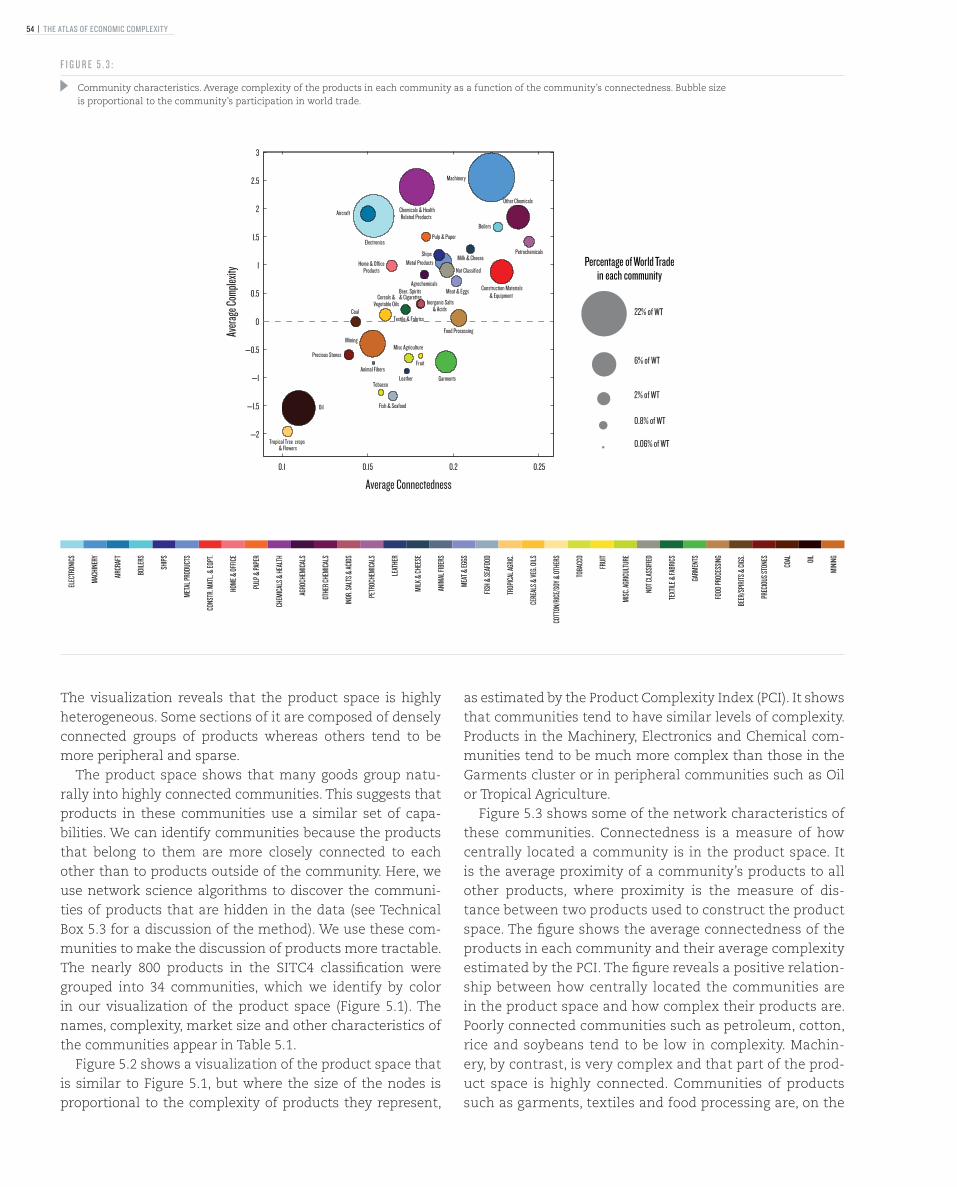
54 | THE ATLAS OF ECONOMIC COMPLEXITY
22% of WT
6% of WT
2% of WT
0.8% of WT
0.06% of WT
Percentage of World Tradein each community
0.1 0.15 0.2 0.25
−2
−1.5
−1
−0.5
0
0.5
1
1.5
2
2.5
3
Average Connectedness
Avera
ge Co
mplex
ity
Machinery
Aircraft
Boilers
ShipsMetal Products
Construction Materials& Equipment
Home & OfficeProducts
Food Processing
Beer, Spirits& Cigarettes
Chemicals & HealthRelated Products
Agrochemicals
Other Chemicals
Inorganic Salts& Acids
Petrochemicals
Pulp & Paper
Textile & Fabrics
Garments
Electronics
Tropical Tree crops& Flowers
Cereals &Vegetable Oils
Tobacco
Fruit
Misc Agriculture
Leather
Milk & Cheese
Animal Fibers
Meat & Eggs
Fish & Seafood
Precious Stones
Coal
Oil
Mining
Not Classified
Community characteristics. Average complexity of the products in each community as a function of the community’s connectedness. Bubble size is proportional to the community’s participation in world trade.
F I G U R E 5 . 3 :
The visualization reveals that the product space is highly heterogeneous. Some sections of it are composed of densely connected groups of products whereas others tend to be more peripheral and sparse.
The product space shows that many goods group natu-rally into highly connected communities. This suggests that products in these communities use a similar set of capa-bilities. We can identify communities because the products that belong to them are more closely connected to each other than to products outside of the community. Here, we use network science algorithms to discover the communi-ties of products that are hidden in the data (see Technical Box 5.3 for a discussion of the method). We use these com-munities to make the discussion of products more tractable. The nearly 800 products in the SITC4 classification were grouped into 34 communities, which we identify by color in our visualization of the product space (Figure 5.1). The names, complexity, market size and other characteristics of the communities appear in Table 5.1.
Figure 5.2 shows a visualization of the product space that is similar to Figure 5.1, but where the size of the nodes is proportional to the complexity of products they represent,
as estimated by the Product Complexity Index (PCI). It shows that communities tend to have similar levels of complexity. Products in the Machinery, Electronics and Chemical com-munities tend to be much more complex than those in the Garments cluster or in peripheral communities such as Oil or Tropical Agriculture.
Figure 5.3 shows some of the network characteristics of these communities. Connectedness is a measure of how centrally located a community is in the product space. It is the average proximity of a community’s products to all other products, where proximity is the measure of dis-tance between two products used to construct the product space. The figure shows the average connectedness of the products in each community and their average complexity estimated by the PCI. The figure reveals a positive relation-ship between how centrally located the communities are in the product space and how complex their products are. Poorly connected communities such as petroleum, cotton, rice and soybeans tend to be low in complexity. Machin-ery, by contrast, is very complex and that part of the prod-uct space is highly connected. Communities of products such as garments, textiles and food processing are, on the
ELEC
TRON
ICS
MACH
INER
Y
AIRCR
AFT
BOILE
RS
SHIP
S
META
L PRO
DUCT
S
CONS
TR. M
ATL.
& EQ
PT.
HOME
& OF
FICE
PULP
& PA
PER
CHEM
ICAL
S & H
EALT
H
AGRO
CHEM
ICAL
S
OTHE
R CHE
MICA
LS
INOR
. SAL
TS &
ACID
S
PETR
OCHE
MICA
LS
LEAT
HER
MILK
& CH
EESE
ANIM
AL FI
BERS
MEAT
& EG
GS
FISH
& SE
AFOO
D
TROP
ICAL
AGRI
C.
CERE
ALS &
VEG.
OILS
COTT
ON/R
ICE/
SOY &
OTHE
RS
TOBA
CCO
FRUI
T
MISC
. AGR
ICUL
TURE
NOT C
LASS
IFIED
TEXT
ILE &
FABR
ICS
GARM
ENTS
FOOD
PROC
ESSI
NG
BEER
/SPI
RITS
& CI
GS.
PREC
IOUS
STON
ES
COAL OI
L
MINI
NG

MAPPING PATHS TO PROSPERITY | 55
T A B L E 5 . 1 :
C H A R A C T E R I S T I C S O F P R O D U C T C O M M U N I T I E S
Community Name Average PCINumber of Products
World Trade World ShareTop 3 Countries by Export
VolumeTop 3 Countries by Num-ber of Products (RCA>1)
Machinery 2.54 125 4.4T 20.29% DEU, USA, JPN DEU, ITA, AUT
Electronics 2.25 52 3.6T 16.71% CHN, HKG, USA CHN, HKG, MYS
Oil -2.08 4 2.3T 10.49% SAU, RUS, NOR EGY, KAZ, DZA
Chemicals & Health 2.52 64 1.6T 7.47% USA, DEU, BEL USA, BEL, DEU
Other Chemicals 1.67 24 1.2T 5.49% DEU, USA, FRA DEU, ITA, ESP
Construction Materials & Equipment 0.77 44 1.1T 5.23% CHN, DEU, ITA CZE, POL, SVN
Mining -0.59 48 1.1T 5.01% AUS, USA, CHL CAN, AUS, KAZ
Garments -0.43 42 1.1T 4.63% CHN, HKG, ITA CHN, VNM, TUN
Food Processing -0.07 26 603B 2.74% DEU, ITA, USA SRB, ESP, BEL
Metal Products 0.76 17 496B 2.26% JPN, DEU, KOR ZAF, UKR, SVK
Aircraft 1.48 10 440B 2.00% FRA, DEU, GBR CAN, GBR, FRA
Not Classified 0.93 36 426B 1.94% USA, CHN, DEU CHN, FRA, GBR
Cereals & Vegetable Oils -0.34 21 295B 1.34% USA, BRA, ARG PRY, MDA, ARG
Home & Office 1.16 23 250B 1.14% CHN, CHE, USA CHN, PAN, PRT
Meat & Eggs 0.64 23 242B 1.10% USA, BRA, DEU FRA, BEL, POL
Ships 0.83 8 232B 1.05% KOR, CHN, JPN ROU, POL, HRV
Petrochemicals 1.22 5 220B 1.00% DEU, USA, BEL PRT, BEL, FRA
Boilers 1.56 14 193B 0.88% CHN, DEU, JPN CHN, TUR, KOR
Fish & Seafood -1.23 11 191B 0.87% CHN, NOR, THA CHL, NAM, SYC
Textile & Fabrics 0.18 32 189B 0.86% CHN, ITA, HKG CHN, TUR, IND
Tropical Agriculture -1.95 16 190B 0.86% IDN, NLD, MYS IDN, CIV, CRI
Coal 0.21 6 183B 0.83% AUS, IDN, RUS CZE, COL, RUS
Misc Agriculture -0.79 22 170B 0.78% BRA, DEU, FRA ESP, TZA, NIC
Precious Stones 0.02 4 170B 0.77% IND, ISR, BEL GBR, LBN, LKA
Pulp & Paper 1.77 11 148B 0.67% USA, CAN, SWE SWE, FIN, CAN
Agrochemicals 0.40 13 141B 0.64% DEU, USA, CAN BEL, JOR, DEU
Milk & Cheese 1.14 7 134B 0.61% DEU, FRA, NLD NLD, BLR, LTU
Beer, Spirits & Cigarettes 0.07 6 124B 0.57% GBR, NLD, DEU JAM, BEL, NLD
Inorganic Salts & Acids -0.22 10 117B 0.53% USA, CHN, DEU ISR, JOR, USA
Cotton, Rice, Soy & Others -2.25 18 96B 0.44% USA, IND, THA TZA, MOZ, GRC
Tobacco -1.46 6 64B 0.29% DEU, NLD, BRA PHL, GRC, SEN
Leather -0.85 14 53B 0.24% ITA, USA, HKG ALB, SOM, ESP
Fruit -0.58 4 45B 0.21% ESP, USA, CHL NLD, LBN, LTU
Animal Fibers -0.85 7 12B 0.06% AUS, CHN, ITA URY, NZL, ZAF

56 | THE ATLAS OF ECONOMIC COMPLEXITY
Complexity Outlook as a function of the Economic Complexity Index and GDP per capita.
F I G U R E 5 . 4 :
F I G U R E 5 . 4 a : F I G U R E 5 . 4 b :
AGO
ALB
ARE
ARG
AUS
AUT
AZE
BEL
BGD
BGR
BIH
BLR
BOL
BRA
BWA
CAN
CHE
CHL
CHN
CIV
VCMR
COG
COL
CRI
CUB
CZE
DNK
DOM
DZA
ECU
EGY
ESP
EST
ETH
FIN
FRA
GAB
GBR
GEOGHA
GIN
GRC
GTM
HKG
HND
HRV HUN
IDN
IND
IRL
IRN
ISRR
ITA
JAM
JORJPN
KAZ
KEN
KGZ
KHM
KOR
KWT
LAO
LBN
LBR
LBY
LKA
LTULVA
MAR MDA
MDG
MEX
MKD
MLIMNG
MOZMRT
MUS
MWI
MYS
NAMNGA
NIC
NLD
NOR
NZL
OMN
PAK
PAN
PER PHL
PNG
POL
PRT
PRYQAT
ROM
RUS
SAU
SDN
SEN
SGP
SLV
SRB
SVKSVN
SWESYR
THA
TJK
TKM TTO
TUN
TUR
TZA
UGA
UKR
URY
USA
UZB
VEN
VNM
YEM
ZAF
ZMB
ZWE
−10
12
3Co
mplex
ity O
utloo
k Ind
ex
−2 −1 0 1 2Economic Complexity Index
AGO
ALB
ARE
ARG
AUS
AUT
AZE
BEL
BGD
BGR
BIH
BLR
BOL
BRA
BWA
CAN
CHE
CHL
CHN
CIV
CMR
COG
COL
CRI
CUB
CZE
DNK
DOM
DZAECU
EGY
ESPEST
ETH
FIN
FRA
GAB
GBR
GEO
GHAGIN
GRC
GTM
HKG
HND
HRVHUN
IDN
IND
IRL
IRN
ISR
ITA
JAM
JOR
JPN
KAZ
KEN
KGZ
KHM
KOR
KWT
LAO
LBN
LBR LBY
LKA
LTULVA
MAR
MDA
MDG
MEX
MKD
MLI
MNGMOZMRT
MUS
MWI
MYS
NAM
NGANIC
NLD
NOR
NZL
OMN
PAK
PAN
PERPHL
PNG
POL
PRT
PRYQAT
ROU
RUS
SAU
SDN
SEN
SGP
SLV
SRB
SVKSVN
SWESYR
THA
TJK
TKMTTO
TUN
TUR
TZA
UGA
UKR
URY
USA
UZB
VEN
VNM
YEM
ZAF
ZMBZWE
−10
12
3
Comp
lexity
Out
look I
ndex
2.5 3 3.5 4 4.5 5
GDP per capita, log [2010]
Com
plex
ity O
utlo
ok In
dex [
2010
]
Com
plex
ity O
utlo
ok In
dex [
2010
]
Economic Complexity Index [2010] GDP per capita, log [2010]
other hand, in an intermediate position, being connected to many products but not very sophisticated. Electronics and Health-Related Chemicals are very complex but not as connected as machinery. This suggests they use specif-ic capabilities relevant within their communities but not outside of them.
We have shown in previous research (Hausmann and Klinger, 2006, 2007 and Hidalgo et al 2007) that the prob-ability that a country will make a new product is strongly related to how close that product is to other products the country already makes. So the location of a country in the product space captures information regarding both the pro-ductive knowledge that it possesses and the capacity to ex-pand that knowledge by moving into other nearby products. The ability of countries to diversify and to move into more complex products is crucially dependent on their initial lo-cation in the product space.
The product space gives us a glimpse of the embedded knowledge countries have by highlighting the productive capabilities they posses and the opportunities these imply. We can evaluate a country’s overall position in the product space by calculating how far it is to alternative products and how complex these products are. We call this measure the Complexity Outlook Index and it can be thought of as the value of the option to move into more and to more com-plex products, given how far they are from a country’s cur-rent position in the product space (see Technical Box 5.4).
Figure 5.4a compares Complexity Outlook with the Eco-nomic Complexity Index. Countries with low levels of com-plexity tend to have few opportunities available. This is because the products they make tend to have few neigh-bors. Complex economies tend to have few remaining
opportunities because they already occupy a large portion of the better part of the product space. Countries with an intermediate level of complexity, on the other hand, differ greatly in their Complexity Outlook. Some countries, like Saudi Arabia, Jamaica and Chile, are located in sparse parts of the product space that imply few easy diversification op-portunities. Others, like India, Greece, Turkey, Brazil and In-donesia are located in parts of the product space where op-portunities are plentiful. Figure 5.4b plots the Complexity Outlook Index against the income per capita of countries. It shows that countries with similar incomes face dramati-cally different opportunities.
Does the position of a country in the product space af-fect how fast its complexity will increase? Said differently, does the Complexity Outlook Index (COI) predict how the Economic Complexity Index (ECI) will evolve? Technical Box 5.5 answers this question in the affirmative. It shows that for both 5- and 10-year horizons, COI has a very strong impact on the growth of ECI. The estimated effects are large and consistent at both horizons.
Finally, we illustrate how countries move through the prod-uct space by looking at Ghana, Poland, Thailand and Turkey (Figure 5.5). Here, highlighted nodes are used to indicate the products that each of these countries was exporting with comparative advantage at each point in time. In all cases we see that new industries –new black squares– tend to lie close to the industries already present in these countries. The pro-ductive transformation undergone by Poland, Thailand and Turkey, however, look striking compared to that of Ghana. Thailand and Turkey, in particular, moved from mostly ag-ricultural societies to manufacturing powerhouses during the 1975-2010 period. Poland, also moved into the center of

MAPPING PATHS TO PROSPERITY | 57
the product space during the last two decades, becoming a manufacturer of most products in both the Home and Of-fice and the Processed Foods community and significantly increasing its participation in the production of machin-ery. These transformations imply an increase in embedded knowledge that is reflected in our Economic Complexity In-dex. Ultimately, it is these transformations that underpinned the impressive growth performance of these countries.
We started this section asking several questions: How does complexity evolve? And how do societies increase the total amount of productive knowledge embedded in them? Here we have shown that countries expand their produc-tive knowledge by moving into nearby goods. This increas-es the likelihood that the effort to accumulate any addi-tional capability will be successful, as the complementary capabilities needed to make a new product are more likely to be present in the production of the nearby goods.
What limits the speed of this process? Since capabili-ties are useful only when combined with others, the ac-cumulation of capabilities is slowed down by the chicken and egg problem. New products may require capabilities that do not exist precisely because the other products that use them are not present. Moreover, since capabilities are chunks of tacit knowledge, accumulating them is difficult
even when there is demand for them, because the country does not have any exemplars to copy.
Most importantly, we must ask why this process of devel-opment occurs in some places but not in others. There are many possible explanations, but our approach adds a new answer to the mix by showing that a country’s position in the product space determines its opportunities to expand its productive knowledge and increase its level of econom-ic complexity. But since the product space is highly het-erogeneous, it confronts countries with radically different opportunities. Ultimately, development is the expansion of the total amount of productive knowledge that is embed-ded in a society , but the process by which this knowledge is accumulated has a structure that, thanks to the product space, we are only now starting to understand.
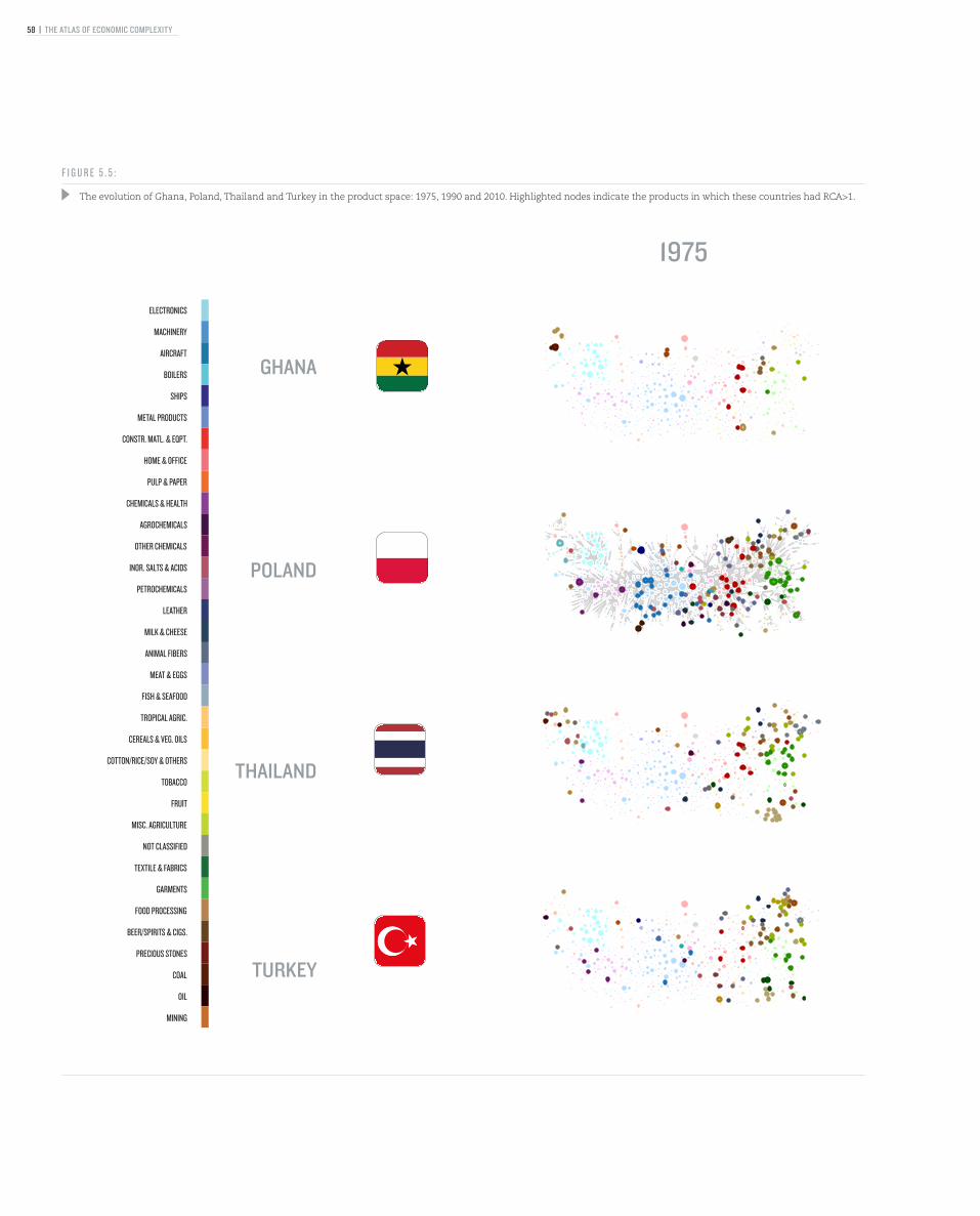
58 | THE ATLAS OF ECONOMIC COMPLEXITY
ELECTRONICS
MACHINERY
AIRCRAFT
BOILERS
SHIPS
METAL PRODUCTS
CONSTR. MATL. & EQPT.
HOME & OFFICE
PULP & PAPER
CHEMICALS & HEALTH
AGROCHEMICALS
OTHER CHEMICALS
INOR. SALTS & ACIDS
PETROCHEMICALS
LEATHER
MILK & CHEESE
ANIMAL FIBERS
MEAT & EGGS
FISH & SEAFOOD
TROPICAL AGRIC.
CEREALS & VEG. OILS
COTTON/RICE/SOY & OTHERS
TOBACCO
FRUIT
MISC. AGRICULTURE
NOT CLASSIFIED
TEXTILE & FABRICS
GARMENTS
FOOD PROCESSING
BEER/SPIRITS & CIGS.
PRECIOUS STONES
COAL
OIL
MINING
1975
GHANA
POLAND
THAILAND
TURKEY
The evolution of Ghana, Poland, Thailand and Turkey in the product space: 1975, 1990 and 2010. Highlighted nodes indicate the products in which these countries had RCA>1.
F I G U R E 5 . 5 :

MAPPING PATHS TO PROSPERITY | 59
1990 2010

60 | THE ATLAS OF ECONOMIC COMPLEXITY
T E C H N I C A L B O X 5 . 2 : V I S U A L I Z I N G T H E P R O D U C T S P A C E
To visualize the product space we use some simple design criteria. First, we want the visualization of the product space to be a connected network. By this, we mean avoiding islands of isolated products. The second criterion is that we want the network visualization to be relatively sparse. Trying to visualize too many links can create unnecessary visual complexity where the most relevant connections will be occluded. This is achieved by creating a visualization in which the average number of links per node is not larger than 5 and results in a representation that can summarize the structure of the product space using the strongest 1% of the links.
To make sure the visualization of the product space is connected, we calcu-late the maximum spanning tree (MST) of the proximity matrix. MST is the set of links that connects all the nodes in the network using a minimum number of connections and the maximum possible sum of proximities. We calculated the MST using Kruskal’s algorithm. Basically the algorithm sorts the values of the proximity matrix in descending order and then includes links in the MST if and
only if they connect an isolated product. By definition, the MST includes all products, but the number of links is the minimum possible.
The second step is to add the strongest connections that were not selected for the MST. In this visualization we included the first 1,006 connections sat-isfying our criterion. By definition a spanning tree for 774 nodes contains 773 edges. With the additional 1,006 connections we end up with 1,779 edges and an average degree of nearly 4.6.
After selecting the links using the above mentioned criteria we build a vi-sualization using a force-directed layout algorithm. In this algorithm nodes repel each other, just like electric charges, while edges act as spring trying to bring connected nodes together. This helps to create a visualization in which densely connected sets of nodes are put together while nodes that are not connected are pushed apart.
Finally, we manually clean up the layout to minimize edge crossings and provide the most clearly representation possible.
Making products requires chunks of embedded knowledge, which we call capa-bilities. The capabilities needed to produce one good may or may not be useful in the production of other goods. Since we do not observe capabilities directly, we create a measure that infers the similarity between the capabilities required by a pair of goods by looking at the probability that they are co-exported. To quantify this similarity we assume that if two goods share most of the requisite capabili-ties, the countries that export one will also export the other. By the same token, goods that do not share many capabilities are less likely to be co-exported.
Our measure is based on the conditional probability that a country that exports product will also export product (Figure 5.1.1). Since conditional probabilities are not symmetric we take the minimum of the probability of ex-porting product , given and the reverse, to make the measure symmetric
Where = 1 if country exports product with RCA>1 and 0 otherwise. is the ubiquity of product .
T E C H N I C A L B O X 5 . 1 : M E A S U R I N G P R O X I M I T Y
and more stringent. For instance, suppose that, 17 countries export wine, 24 export grapes and 11 export both, all with RCA>1. Then, the proximity between wine and grapes is 11/24=0.46. Note that we divide by 24 instead of 17 to re-duce the likelihood that the relationship is spurious. Formally, for a pair of goods and we define proximity as:
ARGENTINA (ARG) GHANA (GHA)
X-RAY MACHINES MEDICAMENTS X-RAY MACHINES MEDICAMENTS
CREAMS AND POLISHESCHEESE FROZEN FISH
CREAMS AND POLISHES
CHEESE FROZEN FISH
NETHERLANDS (NLD)
P = 1
P = 1/2 P = 1/3
An illustration of the method used to calculate proximity.
F I G U R E 5 . 1 . 1 :

MAPPING PATHS TO PROSPERITY | 61
T E C H N I C A L B O X 5 . 3 : I D E N T I F Y I N G P R O D U C T C O M M U N I T I E S
In network science, groups of highly interconnected nodes are known as com-munities. In the product space, communities represent groups of products that are likely to require many of the same capabilities.
We assign products to communities using the algorithm introduced by Ros-vall and Bergstrom (2008). This algorithm finds communities using a two step process. First, it explores the network using a collection of random walkers. The intuition behind this first step is that nodes belonging to the same community are more likely to lie close by in the sequence of nodes visited by a random walk-er. For instance, take photographic film, photographic chemicals and silicones. These are three products that are interconnected and belong to a densely con-nected region of the product space. Hence, the random walker is much more likely to go through the sequences {silicones, photographic chemicals, photo-graphic film} or {photographic film, silicones, photographic chemicals} than {photographic film, grapes, blouses}. The emergence of these sequences in-dicates that photographic film, photographic chemicals and silicones, probably belong to the same community. After several iterations of random walks have been recorded, the algorithm compresses these sequences by looking for ways to rename nodes so as to minimize the amount of space required to store the relevant information about these sequences. For instance, if silicones, photo-graphic films, and photographic chemicals are grouped into a community called photographic materials this would allow compressing the sequence by replac-ing each time it appears by a reference to that community. The algorithm looks for a compression that preserves as much information as possible. This avoids the trivial solution in which all products are assigned to the same community.
The communities determined through this algorithm were manually named and merged into 34 communities (see Table 5.1 for details).
We compare the ability of these communities to summarize the structure of the product space by introducing a measure of community quality. This is the ratio between the average proximity of the links within a community, and those connecting products from that community to products in other communities.
To get a sense of the community quality we compare our assignment of prod-ucts into communities with a baseline null model and three popular categoriza-tions. The baseline null model is given by an ensemble of communities of the same size, where nodes have been assigned to each community at random. In this case the average strength of the links within communities is equal to the average strength of links between communities, and the community quality is 1. The three categorizations we use as comparators are: the first digit of the Stan-dard International Trade Classification, the categories introduced by Leamer (1984) -based on factor intensities- and the technology categories introduced by Lall (2000). All three classifications produce values of the community qual-ity between 1.3 and 1.4, indicating that links within communities tend to be, on average, 30% to 40% stronger than those between communities. The communi-ties we propose here have a community quality value of 1.94, indicating that the links between nodes in the same community are, on average, 94% stronger than those connecting nodes between communities (Figure 5.3.1). The difference in community quality of our proposed community system and that of the three al-ternative categorizations is highly statistically significant with a p-value<1x10-30.
0.0
0.5
1.0
1.5
2.0
1.0+0.005
1.341.36 1.39
1.94
-
Rand
om
SITC
-1 Lall
Leam
er
Comm
unitie
s
Comm
unity
Quali
ty
Community quality. The figure compares the ability of the different classification schemes to capture the structure of the product space.
F I G U R E 5 . 3 . 1 :

62 | THE ATLAS OF ECONOMIC COMPLEXITY
T E C H N I C A L B OX 5 . 4 : U N D E R S TA N D I N G T H E P O S I T I O N O F C O U N T R I E S I N T H E P R O D U C T S PAC E : D I S TA N C E , C O M P L E X I T Y O U T L O O K A N D C O M P L E X I T Y O U T L O O K G A I N
The product space is based on a measure of the similarity of the knowledge set required by products. In this box we develop measures related to the position of countries in the product space. One first measure attempts to capture how far away a product is from a country’s knowledge set, as expressed by its current export basket. This is a measure that relates a country c to a product p that it is not currently exporting in its fair share (see Technical Box 2.2). We call this measure distance and calculate it based on the proportion of knowledge relevant to the product that the country does not have. The knowledge that it does have is captured by the proximity between the products that it is currently making and the particular product of interest . The knowledge that it does not have can be inferred from the proximity between the products that it is currently not making and the product of interest . Distance is, therefore, the sum of the proximities between a particular good and all the products that country is currently not exporting normalized by the sum of proximities between all prod-ucts and product . If country exports most of the goods connected to product , then the distance will be short, close to 0. But, if country only exports a small
proportion of the products that are related to product then the distance will be large (close to 1). Formally,
Where PCI is the Product Complexity Index of product . The term makes sure that we count only the products that the country is not currently producing. Higher Complexity Outlook implies being in the vicinity of more prod-ucts and/or of products that are more complex.
We can use Complexity Outlook to calculate the potential benefit to a coun-try if it were to move to a particular new product. We call this the “Complexity Outlook Gain” that country would obtain from making product . This is calcu-lated as the change in Complexity Outlook that would come as a consequence of developing product . Opportunity gain quantifies the contribution of a new product in terms of opening the doors to more, and more complex products. Formally, we can write the opportunity gain as:Distance gives us an idea of how far each product is relative to a country’s
current mix of exports. Yet, it would be useful to have a holistic measure of the opportunities implied by a country’s position in the product space. We can develop this measure by calculating how close a country is to the products it is currently not effectively making. Here, since more complex products are as-
sociated with higher incomes, it is useful to weigh products by their complex-ity. Some countries may be located near few, poorly connected and relatively simple products, while others may have a rich unexploited nearby neighborhood of highly connected or complex products. This means that countries differ not just in what they make, but also in where their opportunities lie. We can think of this as the value of the option to move into other products.
Hence, to quantify the “Complexity Outlook” of a country’s unexploited pros-pects we sum the “closeness”, i.e. 1 minus the distance, to the products that the country is not currently making weighted by the level of complexity of these products. We can write this mathematically as:

MAPPING PATHS TO PROSPERITY | 63
The Complexity Outlook Index (COI) measures the position of a country in the product space. A country with a higher COI is closer to more complex products that it is not currently making than a country with a lower COI. A country with a higher COI should have an easier time solving the “chicken and egg” problems associated with coordinating the development of new industries and the accumulation of their requisite capabilities. Industries that are closer to a country’s current capabilities should have fewer coordination failures to resolve and hence, provide an easier path to the accumulation of capabilities.
This box explores the effects of the Complexity Outlook Index on the future ECI in 5- and 10-year periods, controlling for the initial value of ECI. Table 5.5.1 shows that for the period 1978-2008, COI is a very strong predictor of future ECI at both horizons.
We can calculate the implied long-run effect of COI on ECI, by assuming that they have a long term relationship of the form:
where represents the long-run effect. We assume that in any period, ECI covers a fraction of the distance between its initial value and its long-term value:
Substituting (2) into (1) we get:
From this equation we can estimate both the long-term effect of COI on ECI ( ) and the speed of adjustment
. The two panels expressed in columns 1 and 2 give
an estimate of of about 0.91 ~ 0.95 and a speed of adjustment
of 8.5 percent in 5 years and 14.3 percent in 10 years, consistent with exponential decay.
We conclude that the Complexity Outlook Index does affect the evolution of the Economic Complexity Index.
T A B L E 5 . 5 . 1
Economic Complexity Index (1978-2008)
5-Year Periods 10-Year Periods
VARIABLES (1) (2)
Initial Economic Complexity Index 0.915*** 0.857***
(0.017) (0.036)
Initial Complexity Outlook Index 0.078*** 0.136***
(0.017) (0.034)
Constant -0.016 -0.064**
(0.035) (0.030)
Observations 637 313
R2 0.926 0.892
Year FE Yes Yes
Speed of adjustment, 0.085 0.143
Long run effect, 0.918 0.951
T E C H N I C A L B O X 5 . 5 : H O W D O E S C O M P L E X I T Y E V O LV E ?
Standard errors clustered by country are shown in parentheses. *** p<0.01, ** p<0.05, * p<0.1

How Can This Atlas Be Used?S E C T I O N 6

MAPPING PATHS TO PROSPERITY | 65
his Atlas is meant to help countries find paths to prosperity. It does so, first, by developing a framework that clarifies what economic devel-opment requires, namely, the accumulation of productive knowledge and its use in both more and more complex industries. Second, The Atlas allows the user to identify development paths that make it easier to coordinate the accumu-lation of new productive capabilities with the
development of the new industries that need them. The Atlas does this by measuring several elements of the
puzzle. It assesses the current state of productive knowledge in any given country, through the Economic Complexity In-dex. It measures how steep the way forward is, as captured by the Complexity Outlook Index. It describes where the country is in the product space, clarifying the diversifica-tion options a country faces. The Atlas describes the neigh-borhood each country finds itself in by pointing out which products are in the “adjacent possible”, how complex they are and how their development would unlock further op-portunities. The country pages included in this Atlas provide a concise look at all these aspects and the Observatory of Economic Complexity permits a deeper exploration online.
This Atlas is, one may say, one more publication that calls
Tattention to an interpretation of the world that, according to the authors, is an important contribution to achieving some commonly shared goal. Other exemplars include freedom, hu-man development, solvency, business environment, competi-tiveness, governance, educational quality, and many others.
Indexes generally do three things. They benchmark per-formance vis-à-vis the best achievers, provide intermediate targets on a path towards a longer-term goal, and offer a guide to action.
As a benchmark, the critical question is whether the index is able to adequately represent the information that it wants to capture. In this respect, in the Economic Complexity Index (ECI), countries improve by increasing the number and com-plexity of the products they successfully export. In the Com-plexity Outlook Index they improve by developing activities that are in parts of the product space that are more connect-ed and that have more complex products. These indicators are based on real data and not on opinion surveys or de jure provisions that may not be important in practice. They have the limitations of the dataset they use: international trade data at a certain level of disaggregation that do not include tradable services or other activities that are not exported.
As an appropriate intermediate target on a path towards a longer-term goal, the question is whether improvements

66 | THE ATLAS OF ECONOMIC COMPLEXITY
in the indicator can be expected to lead to the ultimate goal. If the goal is to accelerate the pace of economic de-velopment, as captured by the growth in GDP per capita, then the Economic Complexity Index and the Complexity Outlook Index do a much better job than the World Eco-nomic Forum’s Global Competitiveness Index or the World Bank’s Governance, Financial Development or Education Indicators. The empirical evidence presented in this Atlas suggests that focusing on improving the complexity indi-cators is a more reliable way to achieve the ultimate goal of faster economic development.
As a guide to action, the question is whether countries can derive recommendations that can offer a clear plan of action to improve the intermediate target. In this respect, indexes differ greatly. At one extreme, the World Bank’s Do-ing Business Index is based on the statutory requirements to perform certain functions. Countries can pretty much figure out which statutory changes will improve their per-formance on the intermediate target. If a country stream-lines the procedure to register a business, it will perform better on the index at the next calculation. Whether this change will actually have any significant economic effect depends on the strength of the connection between the index and the ultimate goal.
On other questions though, such as improving education-al quality, the mapping is not so clear. It is hard to know pre-cisely which changes in current practice would be reflected in better performance. Should schools reduce class size, improve teacher training, increase nutritional assistance or implement standardized exams? Should a country trying to improve rule of law direct its resources to deploying more policemen in the streets, to revamp the judicial system, or to revise their gun laws?
It is important to understand the characteristics of the complexity indexes as guides to action. In the Economic Complexity Index (ECI), countries improve by increasing the number and complexity of the products they success-fully export. In the Complexity Outlook Index they do bet-ter if they move closer to parts of the product space that are denser and that have more complex products. If they do so, they will find it easier to achieve subsequent in-creases in complexity and growth.
But how can countries achieve these changes? As a guide to action, the complexity indexes define the intermediate goals but not the actions that lead to them.
What a country needs to do to increase its complexity is highly specific to its context. The “adjacent possible” of each country is different and the missing productive capabili-

MAPPING PATHS TO PROSPERITY | 67
ties that limit movement to any new industry in the prod-uct space will also be country-specific. In some instances, the provision of better seeds could cause an agricultural revolution; improved infrastructure could open up new possibilities for light manufacturing; clarifying proper-ty rights and human subject regulations may allow for participation in pharmaceutical research; changing the responsiveness of training institutions to the needs of new sectors may unleash their growth. The list goes on. Whether improvements in any of these areas will trigger the desired outcomes in a particular country depends on the presence of the other complementary capabilities that are required for those industries to grow. Countries differ greatly in this dimension. The plan of action must, there-fore, reflect this specificity.
The policy message for most countries is clear: create an environment where a greater diversity of productive activities can thrive, paying particular attention to ac-tivities that are relatively more complex or that open up more opportunities. Countries are more likely to succeed in this agenda if they understand the trade-offs between focusing on products that are close to their current set of productive capabilities vs. focusing on those that may be a bit further away but that offer opportunities for higher
complexity or for subsequent diversification and growth. Nearby products facilitate the identification and provision of missing capabilities, a task that becomes increasingly difficult as the target industry is further away. We therefore accompany our indexes with maps that help chart the op-portunities and rewards available for each country. These are maps that are specific to each country and do not rep-resent one-size-fits-all development advice.
These maps can also be used by firms that are search-ing for a new location or that are looking to diversify into other products. These maps carry information about the productive capabilities that are present in a given country and the degree to which these capabilities are relevant to support other industries.
A map does not tell people where to go, but it does help them determine their destination relative to their current location, and chart their journey towards it. A map em-powers by describing opportunities that would not be ob-vious in the absence of it. If the secret to development is the accumulation of productive knowledge, at a societal rather than individual level, then the process necessarily requires the involvement of many explorers, not just a few planners. This is why the maps we provide in this Atlas are intended for everyone to use.

Which Countries Are Included in This Atlas?S E C T I O N 7

MAPPING PATHS TO PROSPERITY | 69
his Atlas includes data for 128 countries. These account for 99% of world trade, 97% of the world’s total GDP and 95% of the world’s population. To generate this list we used a variety of criteria. First, we limit ourselves only to the set of countries for which there is product-level trade data available in the UN COMTRADE and income data available for 2010. Second, we only use data on countries
with a population above 1,200,000. Third, we only consider countries that exported at least 1 billion dollars per year, on average, between 2006 and 2010. Finally, we remove from this sample Iraq, Macau and Chad, three countries with se-vere data quality issues (Figure 7.1).
Countries are highly heterogeneous. When it comes to the size of their population, territory, income and econ-omy, countries differ by orders of magnitude. When it comes to land, Russia is 1,000 times larger than Kuwait. In terms of population, China is more than 600 times more populous than Slovenia. And as for Gross Domestic Prod-uct, that of the United States is more than 1,300 times larger than Namibia’s. All of these are countries that made it into this Atlas, illustrating the large cross section of the world captured in this book.
TProducts also differ enormously in terms of their world
market size. Depending on the year, crude oil represents five to ten percent of world trade while goat skins repre-sent less than one part in one hundred thousand of total world trade. To make countries and products comparable we control for the size of the country and of the product by calculating their Revealed Comparative Advantage (see Technical Box 2.2). This means that large and small coun-tries and products with big and small markets count the same as far as our method is concerned. Moreover, the data of each country affects the calculations of all oth-ers so including data that is noisy or unreliable greatly af-fects the integrity of our calculations. Countries that are too small in terms of their export base, such as Tuvalu or Vanuatu, or with data that is highly unreliable or not ad-equately classified, do not provide us with a sufficiently broad sample to infer their structure.
Schematic of the procedure used to determine the countries that were included in The Atlas.
F I G U R E 7. 1 :
with GDP and Export information
185 countries
All countries
Population above 1,200,000
147 countries
Trade above $1 Billion
131 countries
Reliable Data (excluding Iraq, Chad and Macau)
128 countries

COMPLEXITY RANKINGS P A R T 2

In this part we present five different rankings. These rankings sort countries according to:
Each of these five rankings captures a different aspect of the world economy. This is well illustrated by the fact very different countries top the rankings for complexity (Japan), ease to increase complexity and growth (India) and past increases in complexity (Mauritius). The heterogeneity of this group shows the wide range of dimensions that are captured by these five different rankings (Table 1). Next, we comment each one of them briefly, and invite readers to explore them by themselves.
R2: Complexity Outlook R3: Per capita Growth Potential R4: Total Growth R5: Change in Complexity
R1: Economic Complexity 0.74 0.42 -0.05 0.32
R2: Complexity Outlook 0.65 0.24 0.44
R3: Per capita Growth Potential 0.75 0.53
R4: Total Growth 0.43
T A B L E 1
Correlations between the five different rankings. The low correlations between the rankings indicate that these tend to capture different dimensions of the world economy.
RANKING 1: Economic Complexity Index (ECI).
RANKING 2: Complexity Outlook Index (COI).
RANKING 3: Expected Growth in Per Capita GDP to 2020.
RANKING 4: Expected GDP Growth to 2020.
RANKING 5: Change in Economic Complexity (1964-2010).