Introduction Model Conclusion and Extensions

The Asset Pricing Implications of Investment inHuman and Physical Capital

Serginio Sylvain

Department of EconomicsUniversity of Chicago

January, 2013

1 / 28

Introduction Model Conclusion and Extensions

Outline

IntroductionMotivation

ModelPrimitivesStatic ConstraintAgent ProblemEquilibriumSolutionProperties of the EquilibriumSummary of the SolutionThe Equity Premium

Conclusion and ExtensionsExtensionsConclusion

2 / 28

Introduction Model Conclusion and Extensions

Motivation

Motivation

“Why is relative distress a state variable of special hedging concern toinvestors? One possible explanation is linked to human capital... [A]negative shock to a distressed firm more likely implies a negative shockto the value of specialized human capital... Thus, workers [may] avoidthe stocks of distressed firms.”–“Multifactor Explanations of Asset Pricing Anomalies”, 1996, Fama andFrench

3 / 28

Introduction Model Conclusion and Extensions

Motivation

I use the approach of Davis et al (2006).

4 / 28

Introduction Model Conclusion and Extensions

Motivation

Pushing beyond Value-Growth, Small-Large...

Figure 2 from Mendez and Sepulveda (2012). The authors also highlight important differences between high-skilled

and low-skilled individuals as well as between the employed and unemployed 5 / 28

Introduction Model Conclusion and Extensions

Motivation

Some recent literature which investigates the asset pricing implications ofcapital allocation or (more generally) asset pricing in a productioneconomy:Jermann (1998), Hall (2000), Kogan (2001,2003), Uligh (2007),Cochrane Longstaff and Santa-Clara (2008), Eberly and Wang(2009,2011), Kozak (2012),...

There is also a (less extensive) literature which studies the implication oflabor supply and labor income on asset pricing:Veronesi and Santos (2005),...

This research shows that production and labor income have importantimplications for asset returns and the predictability of returns. They arealso able to match key moments of asset markets using models withproduction and labor

6 / 28

Introduction Model Conclusion and Extensions

Motivation

I hope to contribute much of this work by highlighting some of themechanisms through which investment in both human and physicalcapital affect asset prices.

For example, during a recession negative shocks to human capital orincreasing uncertainty about the value human capital could make holdingequities less attractive and lead to (counter-cyclical) variations in theequity premium. This may be a plausible alternative to time-varyingrisk-aversion

Some of the questions I would like to address are as follows:

1. What are the implications for returns and predictability of returns?

2. What is the effect of a negative productivity shock on future humancapital accumulation, wage, return on capital, equity and bondreturns?

3. What are the interactions between human capital income, physicalcapital income and equity returns?

7 / 28

Introduction Model Conclusion and Extensions

Primitives

The model uses elements from

Blanchard (1985), Panageas and Garleanu (2010): OLG so that no groupof agents accumulates wealth indefinitely. The endogenous processes willbe bounded and converge to stationary distributions

Panageas and Garleanu (2010): I will use the Martingale approach. Ityields a tractable framework

Eberly and Wang (2009): there are adjustment costs. Empirical evidenceshows that stock market variations is due mostly to variations in pricesrather than the level of capital. Introducing an adjustment cost implies a(time-varying) wedge, qt , between the two (V = qK ) which helps tobetter match data

8 / 28

Introduction Model Conclusion and Extensions

The economy is populated with a continuum of agents.

Each agent faces a constant hazard rate of death π > 0 and a cohort ofmass π is born per unit of time.

The size of the cohort born at time s < t is πe−π(t−s) and the totalpopulation size at date t is

∫ t

−∞ πe−π(t−s) = 1.

A fraction vA of agents are “high-skilled” and will be labelled type A

The remaining agents are of type B (“low-skilled”) and account for afraction vB = 1− vA of the population

The utility function at time t for an agent of type i ∈ {A,B} born attime s is

u(c is,t , h

is,t

)= Log

(c is,th

is,t

)9 / 28

Introduction Model Conclusion and Extensions

The human capital at time t for an agent of type i ∈ {A,B} born at times follows

dhis,this,t

= ΓiLog

(1 +

εis,tθihis,t

)dt − δidt + σidZt

εis,t : investment in human capital on date t

δi : depreciation rate

θi : a scaling constant and Γi ≡ δi

Log(

1+δiθi

)so that the expected growth rate of human capital equals zero whenεis,t = δih

is,t

Lastly, θA > θB and δA < δB so it is more costly for low-skilled agents toaccumulate human capital

10 / 28

Introduction Model Conclusion and Extensions

The two types of agents only differ in the parameters of the adjustmentcost of human capital

As θi →∞ the adjustment cost goes to zero and Et (dhis,t

his,t)→

εis,t

his,tdt

11 / 28

Introduction Model Conclusion and Extensions

The process for physical capital is similar to that of human capital butthe parameters are independent of the agent type. A life insurancecompany also provides πk i

s,t to each agent in return for her physicalcapital at her death

dk is,t

k is,t

= ΓLog

(1 +

e is,tθk i

s,t

)dt − δdt + π + σkdZt

dhis,this,t

= ΓiLog

(1 +

εis,tθihis,t

)dt − δidt + σidZt

dZt introduces aggregate uncertainty and is a standard Brownian Motionincrement.

For now, let us consider a scalar Brownian Motion increment, dZt .

12 / 28

Introduction Model Conclusion and Extensions

There is 1 firm in this economy and it uses human and physical capital inits production process.

For now, assume that the firm can perfectly identify the types of agents.

Aggregate production

Yt = AK 1−αA−αBt

(HA

t

)αA(HB

t

)αB

Aggregate physical capital

Kt =

∫ t

−∞πe−π(t−s)

(vAk

As,t + vBk

Bs,t

)ds

with kAt,t = kB

t,t = K0 for all t

Total human capital of type i ∈ {A,B}

H it =

∫ t

−∞πe−π(t−s)his,tds

with H i0 = hit,t for all t

13 / 28

Introduction Model Conclusion and Extensions

Agents have access to a security that allows to hedge against aggregaterisk. The security price is St and follows

dStSt

= µtdt + ςtdZt

The agents can invest in a risk free bond with return rt as well as therisky security.

ςt , rt and µt will be determined in equilibrium.

Markets are dynamically complete since rank (diag (ςt)) is equal to thenumber of elements in the dZt vector.

At birth, each agent of type i is endowed with physical capital k is,s = K0 ,

human capital his,s = H i0 and financial wealth W i

s,s = W0.

Following Blanchard (1985) and Panageas and Garleanu (2010),W i

s,s = 0 ∀s, i .14 / 28

Introduction Model Conclusion and Extensions

The total wealth is W is,t + qtk

is,t + pith

is,t

{qt , pit}: value (per unit) of physical and human capital, determined inequilibrium.

Rental rate of physical capital is rk,t and the wage rate is ωit

The life insurance company also provides πW is,t to each agent in return

for her financial wealth when at her deathEach agent’s financial wealth process is thus

dW is,t = [$i

s,tWis,tµt + (1−$i

s,t)Wis,trt + πW i

s,t − c is,t − εis,t − e is,t ]dt

+[rk,tkis,t + ωi

this,t ]dt +$i

s,tWis,tςtdZt

Here $is,t : fraction of financial wealth invested in the risk security.

Aggregate financial wealth follows

dWt = πW0dt︸ ︷︷ ︸new births

−πWtdt︸ ︷︷ ︸deaths

+∑

i∈{A,B}

vi

∫ t

−∞πe−π(t−s)

(dW i

s,t

)ds

︸ ︷︷ ︸surviving agents

15 / 28

Introduction Model Conclusion and Extensions

Static Constraint∃ a unique state price density (SPD), Λt , such that Et (ΛTST ) = ΛtSt

dΛt

Λt= −rtdt − σΛ,tdZt

Using Ito’s Lemma we can show that ςt = σΛ,t and µt − rt = σ2Λ,t

Applying Ito’s Lemma to Λte−π(t−s)

(W i

s,t + his,tpit + k i

s,tqt)

andintegrating yields and using a transversality condition yields

W is,s + his,sp

is + ks,sqs

=

Es

∫∞s

Λte−π(t−s)

(c is,t + e is,t + εis,t − rk,tk

is,t − ωth

is,t − πW i

s,t

)dt

+Es

∫∞s

Λte−π(t−s)pith

is,t

(ψ̄i

t

pit− ΓiLog

(1 +

εis,tθihis,t

)+ δi − π

)dt

+Es

∫∞s

Λte−π(t−s)qtk

is,t

(ψt

qt− ΓLog

(1 +

e is,tθk i

s,t

)+ δ − π

)dt

16 / 28

Introduction Model Conclusion and Extensions

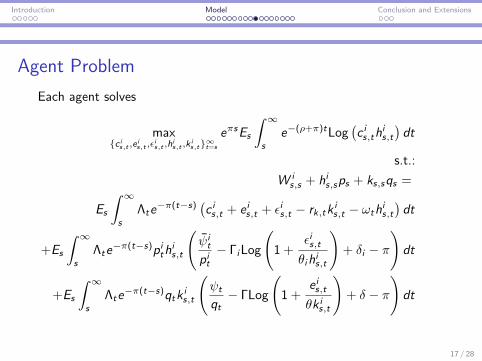
Agent Problem

Each agent solves

max{c is,t ,e is,t ,εis,t ,his,t ,k i

s,t}∞t=s

eπsEs

∫ ∞s

e−(ρ+π)tLog(c is,th

is,t

)dt

s.t.:

W is,s + his,sps + ks,sqs =

Es

∫ ∞s

Λte−π(t−s)

(c is,t + e is,t + εis,t − rk,tk

is,t − ωth

is,t

)dt

+Es

∫ ∞s

Λte−π(t−s)pith

is,t

(ψ̄it

pit− ΓiLog

(1 +

εis,tθihis,t

)+ δi − π

)dt

+Es

∫ ∞s

Λte−π(t−s)qtk

is,t

(ψt

qt− ΓLog

(1 +

e is,tθk i

s,t

)+ δ − π

)dt

17 / 28

Introduction Model Conclusion and Extensions

An equilibrium consists of a set of adapted processes{c is,t , e is,t , εis,t , his,t , k i

s,t , $is,t , p

it , qt , rk,t , ω

it}∀t such that

1. {c is,t , e is,t , εis,t , his,t , k

is,t , $

is,t} solve the agent problem above

2. processes {HAt ,H

Bt ,Kt} maximize the firm’s profit,

Yt − rk,tKt − ωAt H

At − ωB

t HBt

3. market for goods clears:∑i∈{A,B} vi

∫ t

−∞ πe−π(t−s)

(c is,t + e is,t + εis,t

)ds = Yt where

Yt = AK 1−αA−αBt

(HA

t

)αA(HB

t

)αB

4. market for human and physical capital clears:∫ t

−∞ πe−π(t−s)hi

s,tds = H it

for i ∈ {A,B} and∑

i∈{A,B} vi∫ t

−∞ πe−π(t−s)k i

s,tds = Kt

5. market for risky security clears:∑i∈{A,B} vi

∫ t

−∞ πe−π(t−s)$i

s,tWis,tds = St

6. market for bonds clears (zero net bond holdings):∑i∈{A,B} vi

∫ t

−∞ πe−π(t−s)W i

s,t

(1−$i

s,t

)ds = 0

18 / 28

Introduction Model Conclusion and Extensions

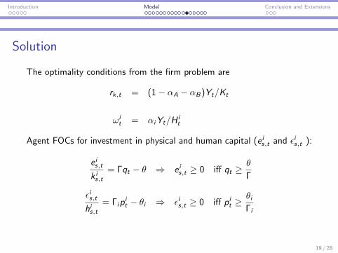
Solution

The optimality conditions from the firm problem are

rk,t = (1− αA − αB)Yt/Kt

ωit = αiYt/H

it

Agent FOCs for investment in physical and human capital (e is,t and εis,t ):

e is,tk is,t

= Γqt − θ ⇒ e is,t ≥ 0 iff qt ≥θ

Γ

εis,this,t

= Γipit − θi ⇒ εis,t ≥ 0 iff pit ≥

θiΓi

19 / 28

Introduction Model Conclusion and Extensions

Thus, pit and qt are the Tobin Q from Q-TheoryTaking the ratio of the FOCs for c is,t and his,t yields

ψ̄it = ωi

t +c is,this,t︸ ︷︷ ︸

marginal benefit from human capital

−(−pt

(ΓiLog

(pt

Γi

θi

)− δi

)+ ptΓi − θi

)︸ ︷︷ ︸

marginal cost to human capital

where the price of human capital is

pit = Et

∫∞t

Λs

Λtψ̄isds

The FOC for k is,t implies

ψt = rk,t︸︷︷︸marginal benefit from physical capital

−(−qt

(ΓLog

(qt

Γk

θk

)− δ)

+ qtΓ− θ)

︸ ︷︷ ︸marginal cost to physical capital

where the price of physical capital is

qt = Et

∫∞t

Λs

Λtψsds

20 / 28

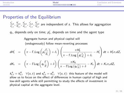
Introduction Model Conclusion and Extensions

Properties of the Equilibriumc is,uc is,t,his,uhis,t,e is,ue is,t,εis,uεis,t,k is,u

k is,t

are independent of s. This allows for aggregation

qt , depends only on time; pit , depends on time and the agent type

Aggregate human and physical capital will

(endogenously) follow mean-reverting processes

dH it =

(π − ΓiLog

(pit

Γi

θi

)+ δi

) πH i0

π − ΓiLog(pit

Γiθi

)+ δi

− H it

dt + H itσidZt

dKt =

(π − ΓLog

(qt

Γ

θ

)+ δ

)(πK0

π − ΓLog(qt

Γθ

)+ δ− Kt

)dt + KtσkdZt

kAs,t = kB

s,t ∀{s, t} and eAs,t = eBs,t ∀{s, t}: this feature of the model willallow us to focus on the effect of differences in human capital of high andlow-skill agents while still permitting to study the effects of investment inphysical capital at the aggregate level.

21 / 28

Introduction Model Conclusion and Extensions

Summarizing the Solutiongiven HA

0 , HB0 , K0 , p0 , qA0 , and qB0 . we can sequentially update the

variables Ct , H it , Kt , pit and qt using

dH it = π

(1−

Γi

πLog

(pit

Γi

θi

)+δi

π

) H i0

1− Γiπ

Log(pit

Γiθi

)+ δi

π

− H it

dt + H itσidZt

dKt = π

(1−

Γ

πLog

(qt

Γ

θ

)+δ

π

) K0

1− Γπ

Log(qt

Γθ

)+ δπ

− Kt

dt + KtσkdZt

dqt =

(−rk,t + qt

(rt + Γ + δ − ΓLog

[qtΓ

θ

])− θ + qtσ

2Λ,t

)dt + qtσΛ,tdZt

dpit =

(−ρ+ π

f it+ pit

(rt + Γi + δi − ΓiLog

[pitΓi

θi

])− θh− ωi

t + pitσ2Λ,t

)dt + pitσΛ,tdZt

rt = g{HAt ,H

Bt ,Kt , p

At , p

Bt , f

At , f

Bt , qt

}σΛ,t = m

{HAt ,H

Bt ,Kt , p

At , p

Bt , qt

}Lastly, εit = H i

t

(Γip

it − θi

), et = Kt (Γqt − θ), Ct = Yt − et −

∑i∈{A,B} vi ε

it 22 / 28

Introduction Model Conclusion and Extensions

f it =his,tW̃ i

s,t

pit solves a linear PDE in {HAt ,H

Bt ,Kt , p

At , p

Bt , qt}

These PDEs are linear, and non-stochastic. They are not difficult tosolve.

We can stack the PDEs into one equation and solve all at once (e.g.Miranda-Fackler).

Here, W̃ is,t is financial wealth plus the present value of the earnings

stream:W̃ i

s,t ≡W is,t + πEt

∫∞t

e−π(τ−t) ΛτΛt

(rk,τk

is,τ + ωi

s,τhis,τ − e is,τ − εis,τ

)dτ

23 / 28

Introduction Model Conclusion and Extensions

The Equity Premium

Et

(dSt

St

)− rt = µt − rt = σ2

Λ,t

where

σΛ,t =Yt

Yt + HAt vAθA + HB

t vBθB + Ktθσy +

Kt (Γqt − θ)

Yt + HAt vAθA + HB

t vBθB + Ktθσk

+HAt

(ΓAp

At − θA

)vA

Yt + HAt vAθA + HB

t vBθB + KtθσA +

HBt

(ΓBp

Bt − θB

)vB

Yt + HAt vAθA + HB

t vBθB + KtθσB

⇒ σΛ,t =Ctσy + εAt

(1 + vAσA

)+ εBt (1 + vBσB) + et (1 + σk )

πW̃t + HAt p

At ΓAvA + HB

t pBt ΓBvB + KtqtΓ

The denominator is a weighted average of financial wealth, human capitalwealth and physical capital wealth

σy = (1− αA − αB )σk + αAσA + αBσB 24 / 28

Introduction Model Conclusion and Extensions

Extensions

We can introduce idiosyncratic shocks in the human capital processes

dhis,this,t

= ΓiLog

(1 +

εis,tθihis,t

)dt − δidt + σidZt +

√ηitdB

is,t

ηit = m(η̄ − ηit)dt − ση√ηitdZt

ση > 0⇒ volatility will be counter cyclical, following some of theresearch from Bloom.

ηit has loading on the aggregate uncertainty. This links idiosyncratic andaggregate risk; akin to Constantinides and Duffie (1996), Di Tella (2012)

LLN implies that idiosyncratic risk will not matter unless there is somefriction: firm cannot perfectly distinguish between the types of agents...

25 / 28

Introduction Model Conclusion and Extensions

We could then study the implications of idiosyncratic risk on low-skill vshigh-skill agents as well as the effects of uncertainty and volatility shockson the wage gap, etc...

The utility function can be changed with little cost. The more generalCRRA utility function would yield the same solution but with thecoefficient of risk aversion appearing is some of the equations.

Since a CRRA utility function ties the agent’s IES to her risk aversion, wecan instead use recursive preferences. More specifically using aEpstein-Zin Kreps-Porteus (EZ-KP) utility function as in Panageas andGarleanu (2010) can be done and would introduce one more PDE.

26 / 28

Introduction Model Conclusion and Extensions

Conclusion

There is an increasing interest in studying the implications of investmentin physical capital on asset pricing.

I hope to complement this research by investigating the joint effects ofinvestment in physical and human capital on asset pricing.

I also hope to study the complementarity between investment in humanand physical capital in a stochastic setting.

The framework presented above is tractable and provides some structurewhich helps formulate interesting questions and determine what to lookfor in data

27 / 28

rt = µy + π − σ2Λ,t −

∑i∈{A,B}

viπβit

+∑

i∈{A,B}

(Γip

it − θiYt

)(H i

t

(v2i π − viΓi

)− viH

i0π)

+Γqt − θ

Yt

(Kt

(π(v2B + v2

A

)− Γ)− K0π

)−

∑i∈{A,B}

H it

YtviΓi

(−ωi

t −π

f it+ pitσΛ,tσ

′

Λ,t

)

−Kt

YtΓ(−rk,t + qtσ

′

Λ,tσΛ,t

)

βit = πφit +

H it

(Γip

it − θi

)+ Kt (Γqt − θ)

Yt

return

0 =∑

i∈{A,B}

∂φi

∂H it

H it

(Γip

it − θi + σi (σy + σΛ,t)

)+

∑i∈{A,B}

1

2

∂2φi

∂(H i

t

)2 Hit

2σ2i

+∂φi

∂KtKt (Γqt − θ + σk (σy + σΛ,t)) +

1

2

∂2φi

∂ (Kt)2 K

2t σ

2k

+∑

i∈{A,B}

∂2φi

∂H it∂Kt

H itσiKtσk +

∂2φi

∂HAt ∂H

Bt

HAt σAσBH

Bt σB

+φi (−rt + µy ,t − σΛ,tσy − π)

{σy , µy}

return

0 =∑

i∈{A,B}

∂f i

∂H it

H it

(Γip

it − θi

)+

∑i∈{A,B}

1

2

∂2f i

∂(H i

t

)2

(H i

t

)2σ2i

+∂f i

∂KtKt (Γqt − θ) +

1

2

∂2f i

∂ (Kt)2 (Kt)

2σ2k

+∑

i∈{A,B}

∂2f i

∂H it∂Kt

H itσiKtσk

+∂2f i

∂HAt ∂H

Bt

HAt σAσBH

Bt σB − (ρ+ π)f i + f it

(ωit − pitΓi + θi

)+ π

return

Introduction Model Conclusion and Extensions

σy = (1− αA − αB)σk + αAσA + αBσB

µy ,t =(−1 + αA + αB)

(−πK0 + Kt

(π + δ − ΓLog

[qtΓθ

]))Kt

+αA

(πHA

0 − HAt

(π + δA + ΓALog

[pAt ΓA

θA

]))HA

t

+β(πHB

0 − HBt

(π + δB + ΓBLog

[pBt ΓB

θB

]))HB

t

+1

2(−1 + αA)αAσ

2A + αAαBσAσB +

1

2(−1 + αB)αBσ

2B

+ (−αA(−1 + αA + αB)σA − αB(−1 + αA + αB)σB)σk

+1

2(−1 + αA + αB)(αA + αB)σ2

k

return

28 / 28