The Assembly Process · The assembly process is considerably simplified if the FEM implementation...
22
25 The Assembly Process 25–1
Transcript of The Assembly Process · The assembly process is considerably simplified if the FEM implementation...
25The Assembly
Process
25–1

Chapter 25: THE ASSEMBLY PROCESS
TABLE OF CONTENTS
Page§25.1 Introduction . . . . . . . . . . . . . . . . . . . . . 25–3
§25.2 Simplifications . . . . . . . . . . . . . . . . . . . . 25–3
§25.3 Simplified Assemblers . . . . . . . . . . . . . . . . . . 25–4§25.3.1 A Plane Truss Example Structure . . . . . . . . . . 25–4§25.3.2 Simplified Assembler Implementation . . . . . . . . . 25–6
§25.4 MET Assemblers . . . . . . . . . . . . . . . . . . . 25–7§25.4.1 A Plane Stress Assembler . . . . . . . . . . . . . 25–7§25.4.2 MET Assembler Implementation . . . . . . . . . . 25–9
§25.5 MET-VFC Assemblers . . . . . . . . . . . . . . . . . 25–10§25.5.1 Node Freedom Arrangement . . . . . . . . . . . . 25–10§25.5.2 Node Freedom Signature . . . . . . . . . . . . . 25–11§25.5.3 The Node Freedom Allocation Table . . . . . . . . . 25–12§25.5.4 The Node Freedom Map Table . . . . . . . . . . . . 25–12§25.5.5 The Element Freedom Signature . . . . . . . . . . 25–13§25.5.6 The Element Freedom Table . . . . . . . . . . . . 25–13§25.5.7 A Plane Trussed Frame Structure . . . . . . . . . . 25–14§25.5.8 MET-VFC Assembler Implementation . . . . . . . . . 25–17
§25.6 *Handling MultiFreedom Constraints . . . . . . . . . . . 25–19
§25. Notes and Bibliography . . . . . . . . . . . . . . . . . 25–20
§25. Exercises . . . . . . . . . . . . . . . . . . . . . . 25–21
25–2

§25.2 SIMPLIFICATIONS
§25.1. Introduction
Chapters 20, 23 and 24 dealt with element level operations. Sandwiched between element processingand solution there is the assembly process that constructs the master stiffness equations. Assemblerexamples for special models were given as recipes in the complete programs of Chapters 21 and22. In the present chapter assembly will be studied with more generality.
The position of the assembler in a DSM-based code for static analysis is sketched in Figure 25.1. Inmost codes the assembler is implemented as a element library loop driver. This means that insteadof forming all elements first and then assembling, the assembler constructs one element at a timein a loop, and immediately merges it into the master equations. This is the merge loop.
Element Stiffness Matrices
Model definition data:geometryelement connectivity materialfabricationfreedom activity
Assembler Equation Solver
Modify Eqsfor BCs
K K
K
^
ELEMENTLIBRARY
Some equation solvers apply BCsand solve simultaneously
To postprocessor
Nodaldisplacements
mergeloop e
Figure 25.1. Role of assembler in FEM program.
Assembly is the most complicated stage of a production finite element program in terms of dataflow. The complexity is not due to mathematical operations, which merely involve matrix addition,but interfacing with a large element library. Forming an element requires access to geometry,connectivity, material, and fabrication data. (In nonlinear analysis, to the state as well.) Mergerequires access to freedom activity data, as well as knowledge of the sparse matrix format in whichK is stored. As illustrated in Figure 25.1, the assembler sits at the crossroads of this data exchange.
The coverage of the assembly process for a general FEM implementation is beyond the scope ofan introductory course. Instead this Chapter takes advantage of assumptions that lead to codingsimplifications. This allows the basic aspects to be covered without excessive delay.
§25.2. Simplifications
The assembly process is considerably simplified if the FEM implementation has these properties:
• All elements are of the same type. For example: all elements are 2-node plane bars.
• The number and configuration of degrees of freedom at each node is the same.
• There are no “gaps” in the node numbering sequence.
• There are no multifreedom constraints treated by master-slave or Lagrange multiplier methods.
• The master stiffness matrix is stored as a full symmetric matrix.
25–3
Chapter 25: THE ASSEMBLY PROCESS
1 (1,2)
1 (1,2)
(1) (2)
(3) (4) (5)
4 (7,8)
4 (7,8)
2 (3,4)
2 (3,4)
3 (5,6)
3 (5,6)
assembly3
x
y
4 4
(1) (2)
(3)(4)
(5)
1 2 3
4
E = 3000 and A = 2 for all bars
(a) (b)
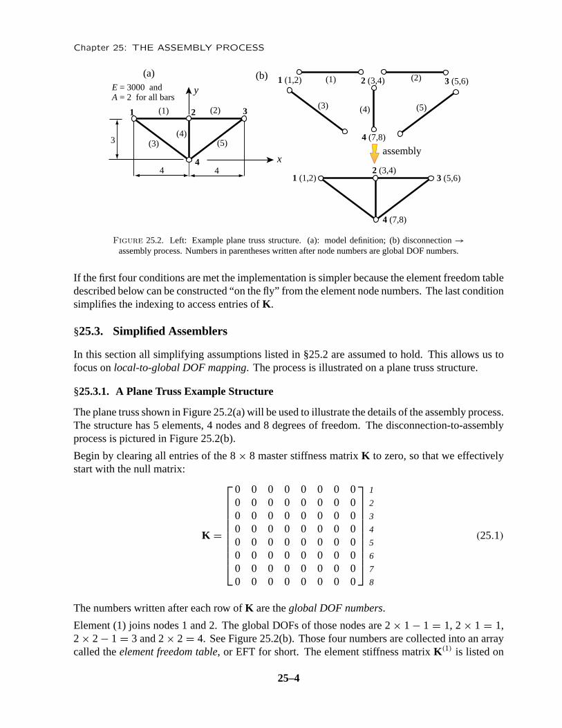
Figure 25.2. Left: Example plane truss structure. (a): model definition; (b) disconnection →assembly process. Numbers in parentheses written after node numbers are global DOF numbers.
If the first four conditions are met the implementation is simpler because the element freedom tabledescribed below can be constructed “on the fly” from the element node numbers. The last conditionsimplifies the indexing to access entries of K.
§25.3. Simplified Assemblers
In this section all simplifying assumptions listed in §25.2 are assumed to hold. This allows us tofocus on local-to-global DOF mapping. The process is illustrated on a plane truss structure.
§25.3.1. A Plane Truss Example Structure
The plane truss shown in Figure 25.2(a) will be used to illustrate the details of the assembly process.The structure has 5 elements, 4 nodes and 8 degrees of freedom. The disconnection-to-assemblyprocess is pictured in Figure 25.2(b).
Begin by clearing all entries of the 8 × 8 master stiffness matrix K to zero, so that we effectivelystart with the null matrix:
K =
0 0 0 0 0 0 0 00 0 0 0 0 0 0 00 0 0 0 0 0 0 00 0 0 0 0 0 0 00 0 0 0 0 0 0 00 0 0 0 0 0 0 00 0 0 0 0 0 0 00 0 0 0 0 0 0 0
1
2
3
4
5
6
7
8
(25.1)
The numbers written after each row of K are the global DOF numbers.
Element (1) joins nodes 1 and 2. The global DOFs of those nodes are 2 × 1 − 1 = 1, 2 × 1 = 1,2 × 2 − 1 = 3 and 2 × 2 = 4. See Figure 25.2(b). Those four numbers are collected into an arraycalled the element freedom table, or EFT for short. The element stiffness matrix K(1) is listed on
25–4
§25.3 SIMPLIFIED ASSEMBLERS
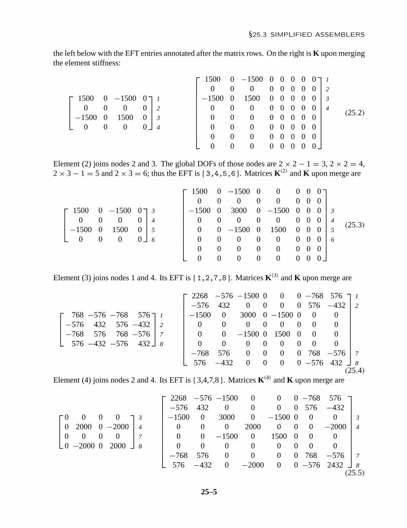
the left below with the EFT entries annotated after the matrix rows. On the right is K upon mergingthe element stiffness:
1500 0 −1500 00 0 0 0
−1500 0 1500 00 0 0 0
1
2
3
4
1500 0 −1500 0 0 0 0 00 0 0 0 0 0 0 0
−1500 0 1500 0 0 0 0 00 0 0 0 0 0 0 00 0 0 0 0 0 0 00 0 0 0 0 0 0 00 0 0 0 0 0 0 00 0 0 0 0 0 0 0
1
2
3
4(25.2)
Element (2) joins nodes 2 and 3. The global DOFs of those nodes are 2 × 2 − 1 = 3, 2 × 2 = 4,2 × 3 − 1 = 5 and 2 × 3 = 6; thus the EFT is { 3,4,5,6 }. Matrices K(2) and K upon merge are
1500 0 −1500 00 0 0 0
−1500 0 1500 00 0 0 0
3
4
5
6
1500 0 −1500 0 0 0 0 00 0 0 0 0 0 0 0
−1500 0 3000 0 −1500 0 0 00 0 0 0 0 0 0 00 0 −1500 0 1500 0 0 00 0 0 0 0 0 0 00 0 0 0 0 0 0 00 0 0 0 0 0 0 0
3
4
5
6
(25.3)
Element (3) joins nodes 1 and 4. Its EFT is { 1,2,7,8 }. Matrices K(3) and K upon merge are
768 −576 −768 576−576 432 576 −432−768 576 768 −576
576 −432 −576 432
1
2
7
8
2268 −576 −1500 0 0 0 −768 576−576 432 0 0 0 0 576 −432−1500 0 3000 0 −1500 0 0 0
0 0 0 0 0 0 0 00 0 −1500 0 1500 0 0 00 0 0 0 0 0 0 0
−768 576 0 0 0 0 768 −576576 −432 0 0 0 0 −576 432
1
2
7
8(25.4)
Element (4) joins nodes 2 and 4. Its EFT is { 3,4,7,8 }. Matrices K(4) and K upon merge are
0 0 0 00 2000 0 −20000 0 0 00 −2000 0 2000
3
4
7
8
2268 −576 −1500 0 0 0 −768 576−576 432 0 0 0 0 576 −432−1500 0 3000 0 −1500 0 0 0
0 0 0 2000 0 0 0 −20000 0 −1500 0 1500 0 0 00 0 0 0 0 0 0 0
−768 576 0 0 0 0 768 −576576 −432 0 −2000 0 0 −576 2432
3
4
7
8(25.5)
25–5

Chapter 25: THE ASSEMBLY PROCESS
Finally, element (5) joins nodes 3 and 4. Its EFT is { 5,6,7,8 }. Matrices K(5) and K upon merge are
768 576 −768 −576576 432 −576 −432
−768 −576 768 576−576 −432 576 432
5
6
7
8
2268 −576 −1500 0 0 0 −768 576−576 432 0 0 0 0 576 −432−1500 0 3000 0 −1500 0 0 0
0 0 0 2000 0 0 0 −20000 0 −1500 0 2268 576 −768 −5760 0 0 0 576 432 −576 −432
−768 576 0 0 −768 −576 1536 0576 −432 0 −2000 −576 −432 0 2864
5
6
7
8(25.6)
Since all elements have been processed, (25.6) is the master stiffness before application of boundaryconditions.
PlaneTrussMasterStiffness[nodxyz_,elenod_,elemat_,elefab_, eleopt_]:=Module[{numele=Length[elenod],numnod=Length[nodxyz], e,ni,nj,eft,i,j,ii,jj,ncoor,Em,A,options,Ke,K}, K=Table[0,{2*numnod},{2*numnod}]; For [e=1, e<=numele, e++, {ni,nj}=elenod[[e]]; eft={2*ni-1,2*ni,2*nj-1,2*nj}; ncoor={nodxyz[[ni]],nodxyz[[nj]]}; Em=elemat[[e]]; A=elefab[[e]]; options=eleopt; Ke=PlaneBar2Stiffness[ncoor,Em,A,options]; For [i=1, i<=4, i++, ii=eft[[i]]; For [j=i, j<=4, j++, jj=eft[[j]]; K[[jj,ii]]=K[[ii,jj]]+=Ke[[i,j]] ]; ]; ]; Return[K] ];
Figure 25.3. Plane truss assembler module.
nodxyz={{-4,3},{0,3},{4,3},{0,0}};elenod= {{1,2},{2,3},{1,4},{2,4},{3,4}};elemat= Table[3000,{5}]; elefab= Table[2,{5}]; eleopt= {True};K=PlaneTrussMasterStiffness[nodxyz,elenod,elemat,elefab,eleopt]; Print["Master Stiffness of Plane Truss of Fig 25.2:"];K=Chop[K]; Print[K//MatrixForm];Print["Eigs of K=",Chop[Eigenvalues[N[K]]]];
2268. −576. −1500. 0 0 0 −768. 576.−576. 432. 0 0 0 0 576. −432.−1500. 0 3000. 0 −1500. 0 0 0
0 0 0 2000. 0 0 0 −2000.0 0 −1500. 0 2268. 576. −768. −576.0 0 0 0 576. 432. −576. −432.
−768. 576. 0 0 −768. −576. 1536. 0576. −432. 0 −2000. −576. −432. 0 2864.
Eigs of K={5007.22, 4743.46, 2356.84, 2228.78, 463.703, 0, 0, 0}
Master Stiffness of Plane Truss of Fig 25.2:
Figure 25.4. Plane truss assembler tester and output results.
25–6
§25.4 MET ASSEMBLERS
§25.3.2. Simplified Assembler Implementation
Figure 25.3 shows a a Mathematica implementation of the assembly process just described. Thisassembler calls the element stiffness module PlaneBar2Stiffness of Figure 20.2. The assembleris invoked by
K = SpaceTrussMasterStiffness[nodxyz,elenod,elemat,elefab,prcopt] (25.7)
The five arguments: nodxyz, elenod, elemat, elefab, and prcopt have the same function asthose described in §21.1.3 for the SpaceTrussMasterStiffness assembler. In fact, comparingthe code in Figure 25.3 to that of Figure 21.1, the similarities are obvious.
Running the script listed in the top of Figure 25.4 produces the output shown in the bottom ofthat figure. The master stiffness (25.6) is reproduced. The eigenvalue analysis verifies that theassembled stiffness has the correct rank of 8 − 3 = 5.
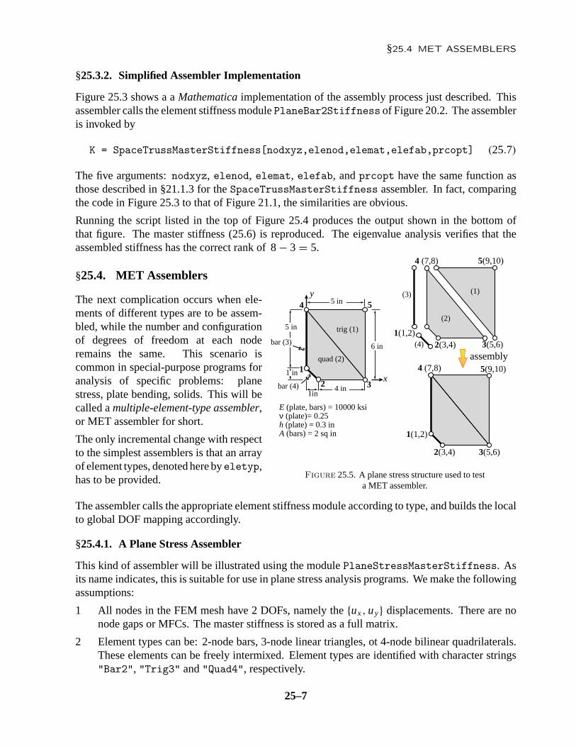
§25.4. MET Assemblers
The next complication occurs when ele-ments of different types are to be assem-bled, while the number and configurationof degrees of freedom at each noderemains the same. This scenario iscommon in special-purpose programs foranalysis of specific problems: planestress, plate bending, solids. This will becalled a multiple-element-type assembler,or MET assembler for short.
The only incremental change with respectto the simplest assemblers is that an arrayof element types, denoted here byeletyp,has to be provided.
1
3
4 5
2
trig (1)
quad (2)
bar (4)
(4)
(3)
bar (3)
E (plate, bars) = 10000 ksiν (plate)= 0.25h (plate) = 0.3 inA (bars) = 2 sq in
6 in
5 in
4 in1in
1 in
5 in
y
x
1(1,2)
1(1,2)
3(5,6)
3(5,6)
4 (7,8)
4 (7,8)
5(9,10)
5(9,10)
2(3,4)
2(3,4)
(2)
(1)
assembly
Figure 25.5. A plane stress structure used to testa MET assembler.
The assembler calls the appropriate element stiffness module according to type, and builds the localto global DOF mapping accordingly.
§25.4.1. A Plane Stress Assembler
This kind of assembler will be illustrated using the module PlaneStressMasterStiffness. Asits name indicates, this is suitable for use in plane stress analysis programs. We make the followingassumptions:
1 All nodes in the FEM mesh have 2 DOFs, namely the {ux , uy} displacements. There are nonode gaps or MFCs. The master stiffness is stored as a full matrix.
2 Element types can be: 2-node bars, 3-node linear triangles, ot 4-node bilinear quadrilaterals.These elements can be freely intermixed. Element types are identified with character strings"Bar2", "Trig3" and "Quad4", respectively.
25–7

Chapter 25: THE ASSEMBLY PROCESS
As noted above, the chief modification over the simplest assembler is that a different stiffnessmodule is invoked as per type. Returned stiffness matrices are generally of different order; in ourcase 4 × 4, 6 × 6 and 8 × 8 for the bar, triangle and quadrilateral, respectively. But the constructionof the EFT is immediate, since node n maps to global freedoms 2n − 1 and 2n. The technique isillustrated with the 4-element, 5-node plane stress structure shown in Figure 25.5. It consists ofone triangle, one quadrilateral, and two bars. The assembly process goes as follows.
Element (1) is a 3-node triangle with nodes 3, 5 and 4, whence the EFT is { 5,6,9,10,7,8 }. Theelement stiffness is
K(1) =
500.0 0 −500.0 −600.0 0 600.00 1333.3 −400.0 −1333.3 400.0 0
−500.0 −400.0 2420.0 1000.0 −1920.0 −600.0−600.0 −1333.3 1000.0 2053.3 −400.0 −720.0
0 400.0 −1920.0 −400.0 1920.0 0600.0 0 −600.0 −720.0 0 720.0
5
6
9
10
7
8
(25.8)
Element (2) is a 4-node quad with nodes 2, 3, 4 and 1, whence the EFT is { 3,4,5,6,7,8,1,2 }.The element stiffness computed with a 2 × 2 Gauss rule is
K(2) =
2076.4 395.55 −735.28 −679.11 −331.78 −136.71 −1009.3 420.27395.55 2703.1 −479.11 −660.61 −136.71 −1191.5 220.27 −850.95
−735.28 −479.11 2067.1 215.82 386.36 427.34 −1718.1 −164.05−679.11 −660.61 215.82 852.12 627.34 358.30 −164.05 −549.81−331.78 −136.71 386.36 627.34 610.92 178.13 −665.50 −668.76−136.71 −1191.5 427.34 358.30 178.13 1433.4 −468.76 −600.15−1009.3 220.27 −1718.1 −164.05 −665.50 −468.76 3393.0 412.54
420.27 −850.95 −164.05 −549.81 −668.76 −600.15 412.54 2000.9
3
4
5
6
7
8
1
2(25.9)
Element (3) is a 2-node bar with nodes 1 and 4, whence the EFT is { 1,2,7,8 }. The elementstiffness is
K(3) =
0 0 0 00 4000.0 0 −4000.00 0 0 00 −4000.0 0 4000.0
1
2
7
8
(25.10)
Element (4) is a 2-node bar with nodes 1 and 2, whence the EFT is { 1,2,3,4 }. The elementstiffness is
K(4) =
7071.1 −7071.1 −7071.1 7071.1−7071.1 7071.1 7071.1 −7071.1−7071.1 7071.1 7071.1 −7071.1
7071.1 −7071.1 −7071.1 7071.1
1
2
3
4
(25.11)
Upon assembly, the master stiffness of the plane stress structure, printed with one digit after the
25–8

§25.4 MET ASSEMBLERS
PlaneStressMasterStiffness[nodxyz_,eletyp_,elenod_, elemat_,elefab_,prcopt_]:=Module[{numele=Length[elenod], numnod=Length[nodxyz],ncoor,type,e,enl,neldof, i,n,ii,jj,eftab,Emat,th,numer,Ke,K}, K=Table[0,{2*numnod},{2*numnod}]; numer=prcopt[[1]]; For [e=1,e<=numele,e++, type=eletyp[[e]]; If [!MemberQ[{"Bar2","Trig3","Quad4"},type], Print["Illegal type", " of element e=",e," Assembly interrupted"]; Return[K]]; enl=elenod[[e]]; n=Length[enl]; eftab=Flatten[Table[{2*enl[[i]]-1,2*enl[[i]]},{i,1,n}]]; ncoor=Table[nodxyz[[enl[[i]]]],{i,n}]; If [type=="Bar2", Em=elemat[[e]]; A=elefab[[e]]; Ke=PlaneBar2Stiffness[ncoor,Em,A,{numer}] ]; If [type=="Trig3", Emat=elemat[[e]]; th=elefab[[e]]; Ke=Trig3IsoPMembraneStiffness[ncoor,Emat,th,{numer}] ]; If [type=="Quad4", Emat=elemat[[e]]; th=elefab[[e]]; Ke=Quad4IsoPMembraneStiffness[ncoor,Emat,th,{numer,2}] ]; neldof=Length[Ke]; For [i=1,i<=neldof,i++, ii=eftab[[i]]; For [j=i,j<=neldof,j++, jj=eftab[[j]]; K[[jj,ii]]=K[[ii,jj]]+=Ke[[i,j]] ]; ]; ]; Return[K]; ];
Figure 25.6. Implementation of MET assembler for plane stress.
decimal point, is
10464.0 −6658.5 −8080.4 7291.3 −1718.1 −164.1 −665.5 −468.8 0 0−6658.5 13072.0 7491.3 −7922.0 −164.1 −549.8 −668.8 −4600.2 0 0−8080.4 7491.3 9147.5 −6675.5 −735.3 −679.1 −331.8 −136.7 0 0
7291.3 −7922.0 −6675.5 9774.1 −479.1 −660.6 −136.7 −1191.5 0 0−1718.1 −164.1 −735.3 −479.1 2567.1 215.8 386.4 1027.3 −500.0 −600.0−164.1 −549.8 −679.1 −660.6 215.8 2185.5 1027.3 358.3 −400.0 −1333.3−665.5 −668.8 −331.8 −136.7 386.4 1027.3 2530.9 178.1 −1920.0 −400.0−468.8 −4600.2 −136.7 −1191.5 1027.3 358.3 178.1 6153.4 −600.0 −720.0
0 0 0 0 −500.0 −400.0 −1920.0 −600.0 2420.0 1000.00 0 0 0 −600.0 −1333.3 −400.0 −720.0 1000.0 2053.3
(25.12)
The eigenvalues of K are
[ 32883. 10517.7 5439.33 3914.7 3228.99 2253.06 2131.03 0 0 0 ] (25.13)
which displays the correct rank.
§25.4.2. MET Assembler Implementation
An implementation of the MET plane stress assembler as a Mathematica module calledPlaneStressMasterStiffness is shown in Figure 25.6. The assembler is invoked by
K = PlaneStressMasterStiffness[nodxyz,eletyp,elenod,elemat,elefab,prcopt](25.14)
The only additional argument is eletyp, which is a list of element types.
25–9
Chapter 25: THE ASSEMBLY PROCESS
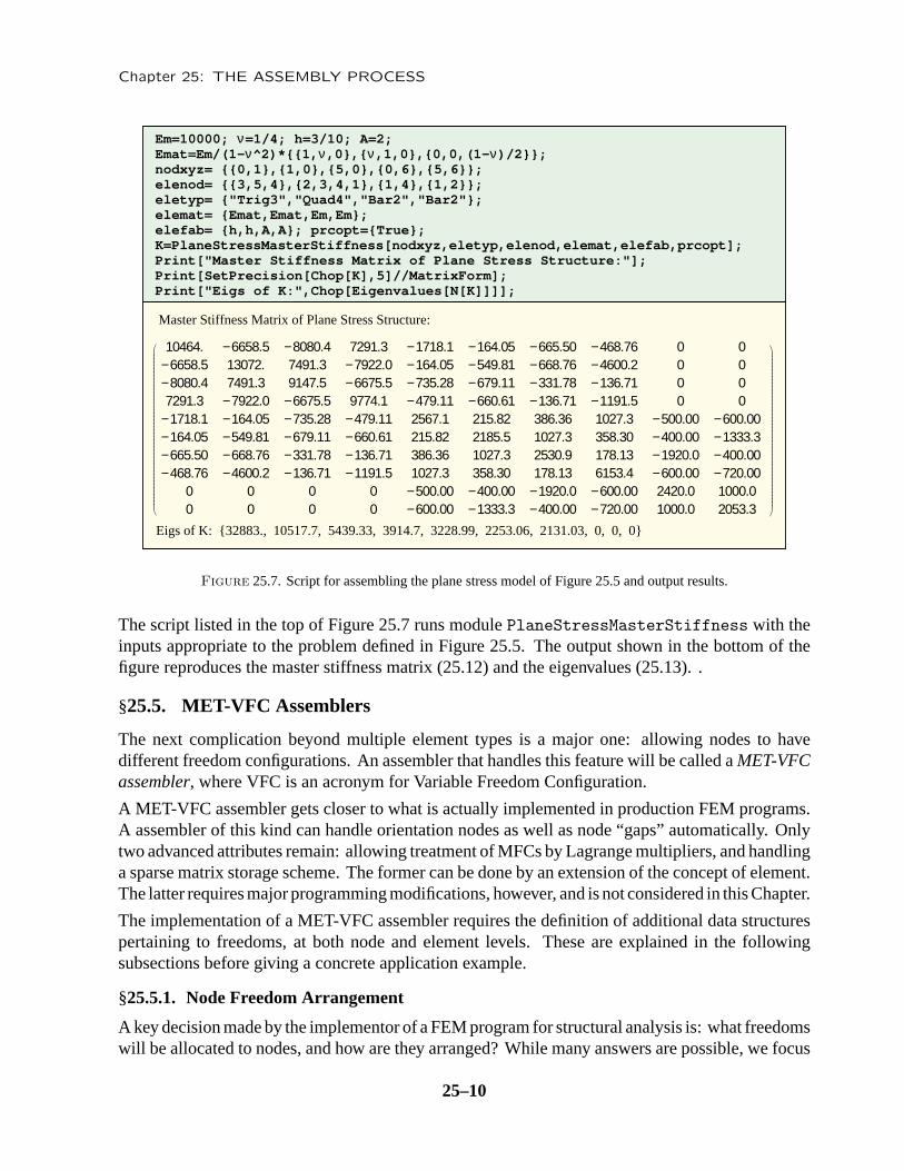
10464. −6658.5 −8080.4 7291.3 −1718.1 −164.05 −665.50 −468.76 0 0−6658.5 13072. 7491.3 −7922.0 −164.05 −549.81 −668.76 −4600.2 0 0−8080.4 7491.3 9147.5 −6675.5 −735.28 −679.11 −331.78 −136.71 0 07291.3 −7922.0 −6675.5 9774.1 −479.11 −660.61 −136.71 −1191.5 0 0
−1718.1 −164.05 −735.28 −479.11 2567.1 215.82 386.36 1027.3 −500.00 −600.00−164.05 −549.81 −679.11 −660.61 215.82 2185.5 1027.3 358.30 −400.00 −1333.3−665.50 −668.76 −331.78 −136.71 386.36 1027.3 2530.9 178.13 −1920.0 −400.00−468.76 −4600.2 −136.71 −1191.5 1027.3 358.30 178.13 6153.4 −600.00 −720.00
0 0 0 0 −500.00 −400.00 −1920.0 −600.00 2420.0 1000.00 0 0 0 −600.00 −1333.3 −400.00 −720.00 1000.0 2053.3
Eigs of K: {32883., 10517.7, 5439.33, 3914.7, 3228.99, 2253.06, 2131.03, 0, 0, 0}
Master Stiffness Matrix of Plane Stress Structure:
Em=10000; ν=1/4; h=3/10; A=2;Emat=Em/(1-ν^2)*{{1,ν,0},{ν,1,0},{0,0,(1-ν)/2}};nodxyz= {{0,1},{1,0},{5,0},{0,6},{5,6}};elenod= {{3,5,4},{2,3,4,1},{1,4},{1,2}};eletyp= {"Trig3","Quad4","Bar2","Bar2"};elemat= {Emat,Emat,Em,Em};elefab= {h,h,A,A}; prcopt={True};K=PlaneStressMasterStiffness[nodxyz,eletyp,elenod,elemat,elefab,prcopt];Print["Master Stiffness Matrix of Plane Stress Structure:"]; Print[SetPrecision[Chop[K],5]//MatrixForm]; Print["Eigs of K:",Chop[Eigenvalues[N[K]]]];
Figure 25.7. Script for assembling the plane stress model of Figure 25.5 and output results.
The script listed in the top of Figure 25.7 runs module PlaneStressMasterStiffness with theinputs appropriate to the problem defined in Figure 25.5. The output shown in the bottom of thefigure reproduces the master stiffness matrix (25.12) and the eigenvalues (25.13). .
§25.5. MET-VFC Assemblers
The next complication beyond multiple element types is a major one: allowing nodes to havedifferent freedom configurations. An assembler that handles this feature will be called a MET-VFCassembler, where VFC is an acronym for Variable Freedom Configuration.
A MET-VFC assembler gets closer to what is actually implemented in production FEM programs.A assembler of this kind can handle orientation nodes as well as node “gaps” automatically. Onlytwo advanced attributes remain: allowing treatment of MFCs by Lagrange multipliers, and handlinga sparse matrix storage scheme. The former can be done by an extension of the concept of element.The latter requires major programming modifications, however, and is not considered in this Chapter.
The implementation of a MET-VFC assembler requires the definition of additional data structurespertaining to freedoms, at both node and element levels. These are explained in the followingsubsections before giving a concrete application example.
§25.5.1. Node Freedom Arrangement
A key decision made by the implementor of a FEM program for structural analysis is: what freedomswill be allocated to nodes, and how are they arranged? While many answers are possible, we focus
25–10
§25.5 MET-VFC ASSEMBLERS
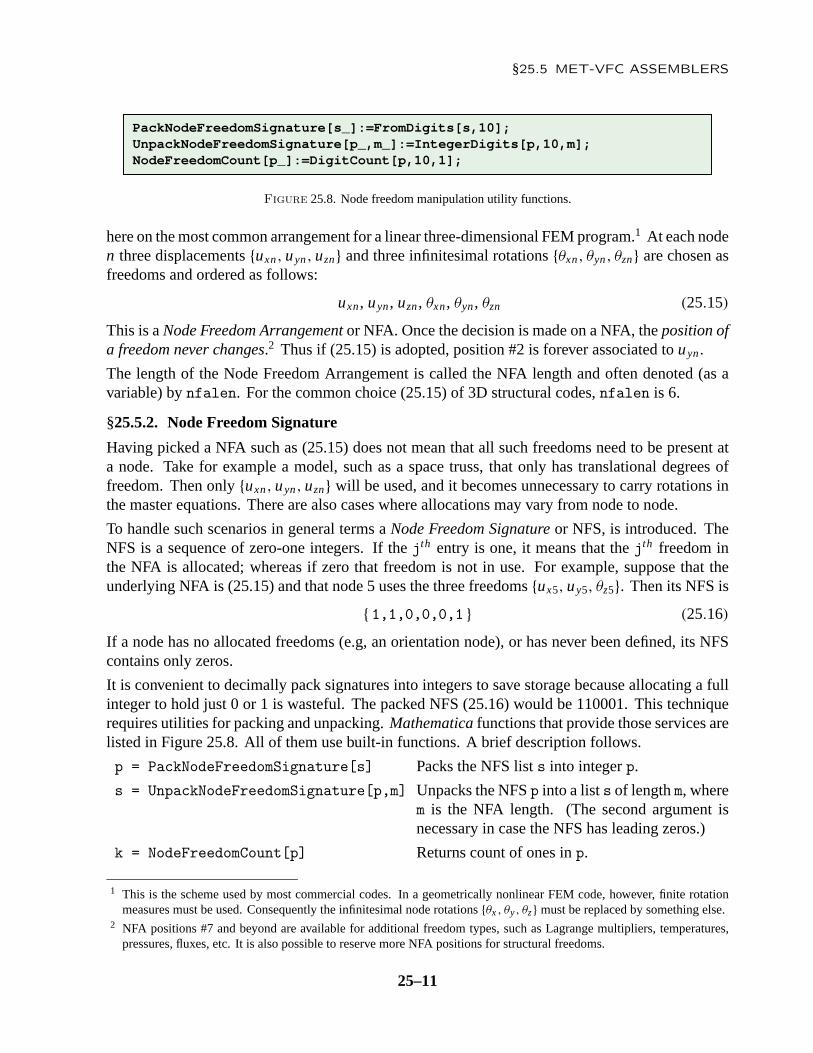
PackNodeFreedomSignature[s_]:=FromDigits[s,10];UnpackNodeFreedomSignature[p_,m_]:=IntegerDigits[p,10,m];NodeFreedomCount[p_]:=DigitCount[p,10,1];
Figure 25.8. Node freedom manipulation utility functions.
here on the most common arrangement for a linear three-dimensional FEM program.1 At each noden three displacements {uxn, uyn, uzn} and three infinitesimal rotations {θxn, θyn, θzn} are chosen asfreedoms and ordered as follows:
uxn , uyn , uzn , θxn , θyn , θzn (25.15)
This is a Node Freedom Arrangement or NFA. Once the decision is made on a NFA, the position ofa freedom never changes.2 Thus if (25.15) is adopted, position #2 is forever associated to uyn .
The length of the Node Freedom Arrangement is called the NFA length and often denoted (as avariable) by nfalen. For the common choice (25.15) of 3D structural codes, nfalen is 6.
§25.5.2. Node Freedom Signature
Having picked a NFA such as (25.15) does not mean that all such freedoms need to be present ata node. Take for example a model, such as a space truss, that only has translational degrees offreedom. Then only {uxn, uyn, uzn} will be used, and it becomes unnecessary to carry rotations inthe master equations. There are also cases where allocations may vary from node to node.
To handle such scenarios in general terms a Node Freedom Signature or NFS, is introduced. TheNFS is a sequence of zero-one integers. If the jth entry is one, it means that the jth freedom inthe NFA is allocated; whereas if zero that freedom is not in use. For example, suppose that theunderlying NFA is (25.15) and that node 5 uses the three freedoms {ux5, uy5, θz5}. Then its NFS is
{ 1,1,0,0,0,1 } (25.16)
If a node has no allocated freedoms (e.g, an orientation node), or has never been defined, its NFScontains only zeros.
It is convenient to decimally pack signatures into integers to save storage because allocating a fullinteger to hold just 0 or 1 is wasteful. The packed NFS (25.16) would be 110001. This techniquerequires utilities for packing and unpacking. Mathematica functions that provide those services arelisted in Figure 25.8. All of them use built-in functions. A brief description follows.
p = PackNodeFreedomSignature[s] Packs the NFS list s into integer p.
s = UnpackNodeFreedomSignature[p,m] Unpacks the NFS p into a list s of length m, wherem is the NFA length. (The second argument isnecessary in case the NFS has leading zeros.)
k = NodeFreedomCount[p] Returns count of ones in p.
1 This is the scheme used by most commercial codes. In a geometrically nonlinear FEM code, however, finite rotationmeasures must be used. Consequently the infinitesimal node rotations {θx , θy , θz} must be replaced by something else.
2 NFA positions #7 and beyond are available for additional freedom types, such as Lagrange multipliers, temperatures,pressures, fluxes, etc. It is also possible to reserve more NFA positions for structural freedoms.
25–11

Chapter 25: THE ASSEMBLY PROCESS
NodeFreedomMapTable[nodfat_]:=Module[{numnod=Length[nodfat], i,nodfmt}, nodfmt=Table[0,{numnod}]; For [i=1,i<=numnod-1,i++, nodfmt[[i+1]]=nodfmt[[i]]+ DigitCount[nodfat[[i]],10,1] ]; Return[nodfmt]];
TotalFreedomCount[nodfat_]:=Sum[DigitCount[nodfat[[i]],10,1], {i,Length[nodfat]}];
Figure 25.9. Modules to construct the NFMT from the NFAT, and to compute the total number of freedoms.
Example 25.1. PackNodeFreedomSignature[{ 1,1,0,0,0,1 }] returns 110001. The inverse isUnpackNodeFreedomSignature[110001,6], which returns { 1,1,0,0,0,1 }.NodeFreedomCount[110001] returns 3.
§25.5.3. The Node Freedom Allocation Table
The Node Freedom Allocation Table, or NFAT, is a node by node list of packed node freedomsignatures. In Mathematica the list containing this table is internally identified as nodfat. Theconfiguration of the NFAT for the plane stress example structure of Figure 25.5 is
nodfat = { 110000,110000,110000,110000,110000 } = Table[110000,{ 5 }]. (25.17)
This says that only two freedoms: {ux , uy}, are used at each of the five nodes.
A zero entry in the NFAT flags a node with no allocated freedoms. This is either an orientationnode, or an undefined one. The latter case happens when there is a node numbering gap, which is acommon occurence when certain mesh generators are used. In the case of a MET-VFC assemblersuch gaps are not considered errors.
§25.5.4. The Node Freedom Map Table
The Node Freedom Map Table, or NFMT, is an array with one entry per node. Suppose that noden has k ≥ 0 allocated freedoms. These have global equation numbers i + j , j = 1, . . . , k. This iis called the base equation index: it represent the global equation number before the first equationto which node n contributes. Obviously i = 0 if n = 1. Base equation indices for all nodes arerecorded in the NFMT.3
In Mathematica code the table is internally identified as nodfmt. Figure 25.9 lists a module thatconstructs the NFMT given the NFAT. It is invoked as
nodfmt = NodeFreedomMapTable[nodfat] (25.18)
The only argument is the NFAT. The module builds the NFMT by simple incrementation, andreturns it as function value.
3 The “map” qualifier comes from the use of this array in computing element-to-global equation mapping.
25–12
§25.5 MET-VFC ASSEMBLERS
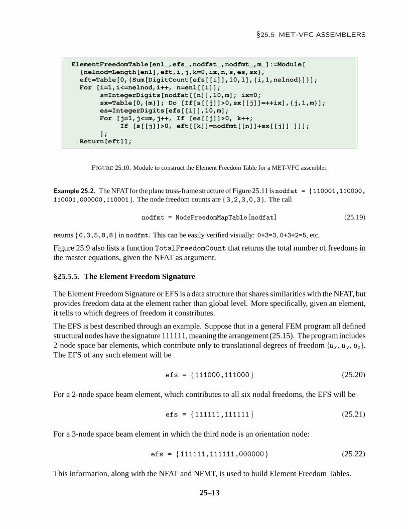
ElementFreedomTable[enl_,efs_,nodfat_,nodfmt_,m_]:=Module[ {nelnod=Length[enl],eft,i,j,k=0,ix,n,s,es,sx}, eft=Table[0,{Sum[DigitCount[efs[[i]],10,1],{i,1,nelnod}]}]; For [i=1,i<=nelnod,i++, n=enl[[i]]; s=IntegerDigits[nodfat[[n]],10,m]; ix=0; sx=Table[0,{m}]; Do [If[s[[j]]>0,sx[[j]]=++ix],{j,1,m}]; es=IntegerDigits[efs[[i]],10,m]; For [j=1,j<=m,j++, If [es[[j]]>0, k++; If [s[[j]]>0, eft[[k]]=nodfmt[[n]]+sx[[j]] ]]]; ]; Return[eft]];
Figure 25.10. Module to construct the Element Freedom Table for a MET-VFC assembler.
Example 25.2. The NFAT for the plane truss-frame structure of Figure 25.11 isnodfat = { 110001,110000,110001,000000,110001 }. The node freedom counts are { 3,2,3,0,3 }. The call
nodfmt = NodeFreedomMapTable[nodfat] (25.19)
returns { 0,3,5,8,8 } in nodfmt. This can be easily verified visually: 0+3=3, 0+3+2=5, etc.
Figure 25.9 also lists a function TotalFreedomCount that returns the total number of freedoms inthe master equations, given the NFAT as argument.
§25.5.5. The Element Freedom Signature
The Element Freedom Signature or EFS is a data structure that shares similarities with the NFAT, butprovides freedom data at the element rather than global level. More specifically, given an element,it tells to which degrees of freedom it constributes.
The EFS is best described through an example. Suppose that in a general FEM program all definedstructural nodes have the signature 111111, meaning the arrangement (25.15). The program includes2-node space bar elements, which contribute only to translational degrees of freedom {ux , uy, uz}.The EFS of any such element will be
efs = { 111000,111000 } (25.20)
For a 2-node space beam element, which contributes to all six nodal freedoms, the EFS will be
efs = { 111111,111111 } (25.21)
For a 3-node space beam element in which the third node is an orientation node:
efs = { 111111,111111,000000 } (25.22)
This information, along with the NFAT and NFMT, is used to build Element Freedom Tables.
25–13

Chapter 25: THE ASSEMBLY PROCESS
§25.5.6. The Element Freedom Table
The Element Freedom Table or EFT has been encountered in all previous assembler examples. Itis a one dimensional list of length equal to the number of element DOF. If the ith element DOFmaps to the kth global DOF, then the ith entry of EFT contains k. This allows to write the mergeloop compactly. In the simpler assemblers discussed in previous sections, the EFT can be built “onthe fly” simply from element node numbers. For a MET-VFC assembler that is no longer the case.To take care of the VFC feature, the construction of the EFT is best done by a separate module. AMathematica implementation is shown in Figure 25.10. Discussion of the logic, which is not trivial,is relegated to an Exercise, and we simply describe here the interface. The module is invoked as
eft = ElementFreedomTable[enl,efs,nodfat,nodfmt,m] (25.23)
The arguments are
enl The element node list.
efs The Element Freedom Signature (EFS) list.
nodfat The Node Freedom Allocation Table (NFAT) described in 25.5.3
nodfmt The Node Freedom Map Table (NFMT) described in 25.5.4
m The NFA length, often 6.
The module returns the Element Freedom Table as function value. Examples of use of this moduleare provided in the plane trussed frame example below.
Remark 25.1. The EFT constructed by ElementFreedomTable is guaranteed to contain only positive entriesif every freedom declared in the EFS matches a globally allocated freedom in the NFAT. But it is possiblefor the returned EFT to contain zero entries. This can only happen if an element freedom does not match aglobally allocated one. For example suppose that a 2-node space beam element with the EFS (25.21) is placedinto a program that does not accept rotational freedoms and thus has a NFS of 111000 at all structural nodes.Then six of the EFT entries, namely those pertaining to the rotational freedoms, would be zero.
The occurrence of a zero entry in a EFT normally flags a logic or input data error. If detected, the assemblershould print an appropriate error message and abort. The module of Figure 25.10 does not make that decisionbecause it lacks certain information, such as the element number, that should be placed into the message.
§25.5.7. A Plane Trussed Frame Structure
To illustrate the workings of a MET-VFC assembler we will follow the assembly process of thestructure pictured in Figure 25.11(a). The finite element discretization, element disconnection andassembly process are illustrated in Figure 25.11(b,c,d). Although the structure is chosen to be planeto facilitate visualization, it will be considered within the context of a general purpose 3D programwith the freedom arrangement (25.15) at each node.
The structure is a trussed frame. It uses two element types: plane (Bernoulli-Euler) beam-columnsand plane bars. Geometric, material and fabrication data are given in Figure 25.11(a). The FEMidealization has 4 nodes and 5 elements. Nodes numbers are 1, 2, 3 and 5 as shown in Figure 25.11(b).Node 4 is purposedly left out to illustrate handling of numbering gaps. There are 11 DOFs, three
25–14

§25.5 MET-VFC ASSEMBLERS
BarBar
Bar
1
1(1,2,3)1(1,2,3)
2
3(6,7,8)3(6,7,8)
5
5(9,10,11)5(9,10,11)
3
2(4,5)2(4,5)
(a)
(b)
(c) (d)
disassembly
assembly
FEM idealization
(1) (2)
(3) (4) (5)
Beam-column Beam-column
3 m
E=200000 MPa A=0.003 m2
(node 4: undefined)
E=200000 MPa A=0.001 m 2
E=200000 MPa A=0.001 m2
2E=30000 MPa, A=0.02 m , I =0.0004 m4zz
4 m 4 m
x
y
x
y
Figure 25.11. Trussed frame structure to illustrate a MET-VFC assembler: (a) original structureshowing dimensions, material and fabrication properties; (b) finite element idealization with bars andbeam column elements; (c) conceptual disassembly; (d) assembly. Numbers written in parentheses
after a node number in (c,d) are the global freedom (equation) numbers allocated to that node.
at nodes 1, 3 and 5, and two at node 2. They are ordered as
Global DOF #: 1 2 3 4 5 6 7 8 9 10 11DOF: ux1 uy1 θz1 ux2 uy2 ux3 uy3 θz3 ux5 uy5 θz5
Node #: 1 1 1 2 2 3 3 3 5 5 5(25.24)
The NFAT and NFMT can be constructed by inspection of (25.24) to be
nodfat = { 110001,110000,110001,000000,110001 }nodfmt = { 0,3,5,8,8 } (25.25)
The element freedom data structures can be also constructed by inspection:
Elem Type Nodes EFS EFT
(1) Beam-column { 1,3 } { 110001,110001 } { 1,2,3,6,7,8 }(2) Beam-column { 3,5 } { 110001,110001 } { 6,7,8,9,10,11 }(3) Bar { 1,2 } { 110000,110000 } { 1,2,4,5 }(4) Bar { 2,3 } { 110000,110000 } { 4,5,6,7 }(5) Bar { 2,5 } { 110000,110000 } { 4,5,9,10 } (25.26)
Next we list the element stiffness matrices, computed with the modules discussed in Chapter 20.The EFT entries are annotated as usual.
25–15

Chapter 25: THE ASSEMBLY PROCESS
Element (1): This is a plane beam-column element with stiffness
K(1) =
150. 0. 0. −150. 0. 0.
0. 22.5 45. 0. −22.5 45.
0. 45. 120. 0. −45. 60.
−150. 0. 0. 150. 0. 0.
0. −22.5 −45. 0. 22.5 −45.
0. 45. 60. 0. −45. 120.
1
2
3
6
7
8
(25.27)
Element (2): This is a plane beam-column with element stiffness identical to the previous one
K(2) =
150. 0. 0. −150. 0. 0.
0. 22.5 45. 0. −22.5 45.
0. 45. 120. 0. −45. 60.
−150. 0. 0. 150. 0. 0.
0. −22.5 −45. 0. 22.5 −45.
0. 45. 60. 0. −45. 120.
6
7
8
9
10
11
(25.28)
Element (3): This is a plane bar element with stiffness
K(3) =
25.6 −19.2 −25.6 19.2−19.2 14.4 19.2 −14.4−25.6 19.2 25.6 −19.219.2 −14.4 −19.2 14.4
1
2
4
5
(25.29)
Element (4): This is a plane bar element with stiffness
K(4) =
0 0 0 00 200. 0 −200.
0 0 0 00 −200. 0 200.
4
5
6
7
(25.30)
Element (5): This is a plane bar element with stiffness
K(5) =
25.6 19.2 −25.6 −19.219.2 14.4 −19.2 −14.4
−25.6 −19.2 25.6 19.2−19.2 −14.4 19.2 14.4
4
5
9
10
(25.31)
Upon merging the 5 elements the master stiffness matrix becomes
K =
175.6 −19.2 0 −25.6 19.2 −150. 0 0 0 0 0−19.2 36.9 45. 19.2 −14.4 0 −22.5 45. 0 0 0
0 45. 120. 0 0 0 −45. 60. 0 0 0−25.6 19.2 0 51.2 0 0 0 0 −25.6 −19.2 0
19.2 −14.4 0 0 228.8 0 −200. 0 −19.2 −14.4 0−150. 0 0 0 0 300. 0 0 −150. 0 0
0 −22.5 −45. 0 −200. 0 245. 0 0 −22.5 45.
0 45. 60. 0 0 0 0 240. 0 −45. 60.
0 0 0 −25.6 −19.2 −150. 0 0 175.6 19.2 00 0 0 −19.2 −14.4 0 −22.5 −45. 19.2 36.9 −45.
0 0 0 0 0 0 45. 60. 0 −45. 120.
1
2
3
4
5
6
7
8
9
10
11(25.32)
25–16
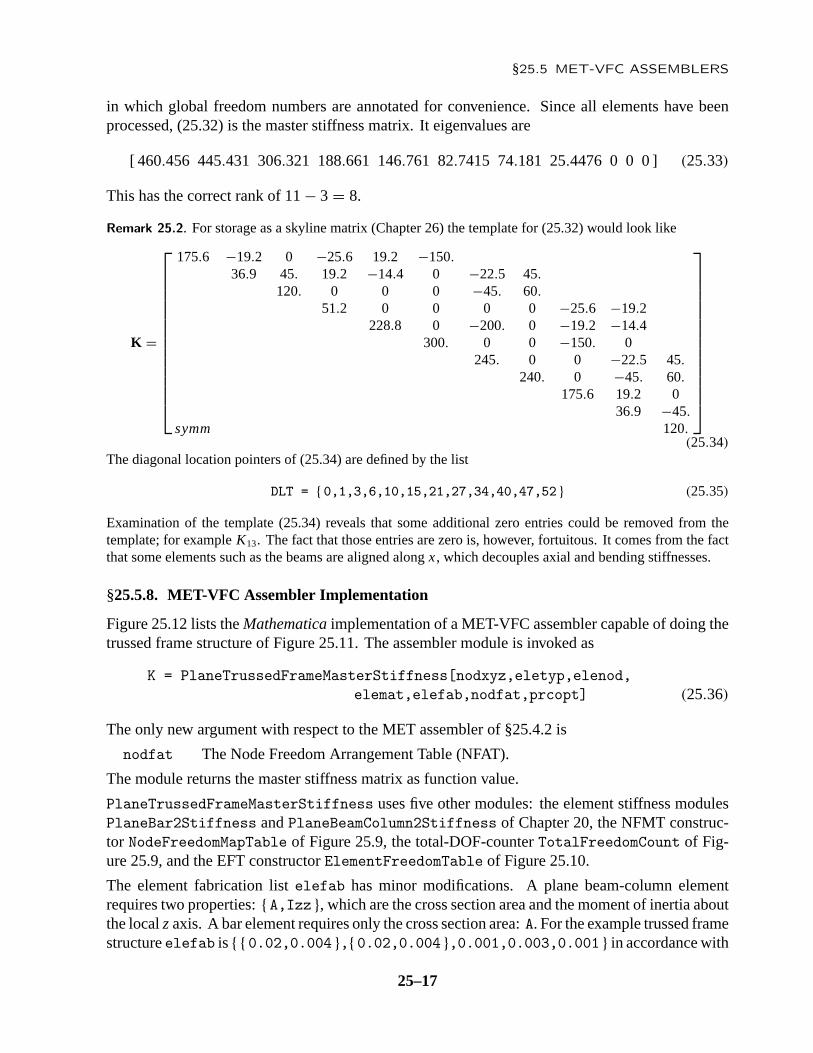
§25.5 MET-VFC ASSEMBLERS
in which global freedom numbers are annotated for convenience. Since all elements have beenprocessed, (25.32) is the master stiffness matrix. It eigenvalues are
[ 460.456 445.431 306.321 188.661 146.761 82.7415 74.181 25.4476 0 0 0 ] (25.33)
This has the correct rank of 11 − 3 = 8.
Remark 25.2. For storage as a skyline matrix (Chapter 26) the template for (25.32) would look like
K =
175.6 −19.2 0 −25.6 19.2 −150.
36.9 45. 19.2 −14.4 0 −22.5 45.
120. 0 0 0 −45. 60.
51.2 0 0 0 0 −25.6 −19.2228.8 0 −200. 0 −19.2 −14.4
300. 0 0 −150. 0245. 0 0 −22.5 45.
240. 0 −45. 60.
175.6 19.2 036.9 −45.
symm 120.
(25.34)
The diagonal location pointers of (25.34) are defined by the list
DLT = { 0,1,3,6,10,15,21,27,34,40,47,52 } (25.35)
Examination of the template (25.34) reveals that some additional zero entries could be removed from thetemplate; for example K13. The fact that those entries are zero is, however, fortuitous. It comes from the factthat some elements such as the beams are aligned along x , which decouples axial and bending stiffnesses.
§25.5.8. MET-VFC Assembler Implementation
Figure 25.12 lists the Mathematica implementation of a MET-VFC assembler capable of doing thetrussed frame structure of Figure 25.11. The assembler module is invoked as
K = PlaneTrussedFrameMasterStiffness[nodxyz,eletyp,elenod,elemat,elefab,nodfat,prcopt] (25.36)
The only new argument with respect to the MET assembler of §25.4.2 is
nodfat The Node Freedom Arrangement Table (NFAT).
The module returns the master stiffness matrix as function value.
PlaneTrussedFrameMasterStiffness uses five other modules: the element stiffness modulesPlaneBar2Stiffness and PlaneBeamColumn2Stiffness of Chapter 20, the NFMT construc-tor NodeFreedomMapTable of Figure 25.9, the total-DOF-counter TotalFreedomCount of Fig-ure 25.9, and the EFT constructor ElementFreedomTable of Figure 25.10.
The element fabrication list elefab has minor modifications. A plane beam-column elementrequires two properties: { A,Izz }, which are the cross section area and the moment of inertia aboutthe local z axis. A bar element requires only the cross section area: A. For the example trussed framestructure elefab is { { 0.02,0.004 },{ 0.02,0.004 },0.001,0.003,0.001 } in accordance with
25–17
Chapter 25: THE ASSEMBLY PROCESS
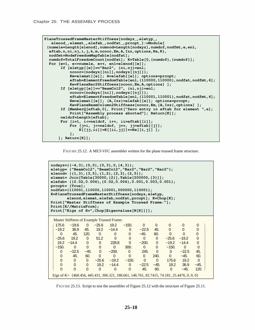
PlaneTrussedFrameMasterStiffness[nodxyz_,eletyp_, elenod_,elemat_,elefab_,nodfat_,prcopt_]:=Module[ {numele=Length[elenod],numnod=Length[nodxyz],numdof,nodfmt,e,enl, eftab,n,ni,nj,i,j,k,m,ncoor,Em,A,Izz,options,Ke,K}, nodfmt=NodeFreedomMapTable[nodfat]; numdof=TotalFreedomCount[nodfat]; K=Table[0,{numdof},{numdof}]; For [e=1, e<=numele, e++, enl=elenod[[e]]; If [eletyp[[e]]=="Bar2", {ni,nj}=enl; ncoor={nodxyz[[ni]],nodxyz[[nj]]}; Em=elemat[[e]]; A=elefab[[e]]; options=prcopt; eftab=ElementFreedomTable[enl,{110000,110000},nodfat,nodfmt,6]; Ke=PlaneBar2Stiffness[ncoor,Em,A,options] ]; If [eletyp[[e]]=="BeamCol2", {ni,nj}=enl; ncoor={nodxyz[[ni]],nodxyz[[nj]]}; eftab=ElementFreedomTable[enl,{110001,110001},nodfat,nodfmt,6]; Em=elemat[[e]]; {A,Izz}=elefab[[e]]; options=prcopt; Ke=PlaneBeamColumn2Stiffness[ncoor,Em,{A,Izz},options] ]; If [MemberQ[eftab,0], Print["Zero entry in eftab for element ",e]; Print["Assembly process aborted"]; Return[K]]; neldof=Length[eftab]; For [i=1, i<=neldof, i++, ii=eftab[[i]]; For [j=i, j<=neldof, j++, jj=eftab[[j]]; K[[jj,ii]]=K[[ii,jj]]+=Ke[[i,j]] ]; ]; ]; Return[K]];
Figure 25.12. A MET-VFC assembler written for the plane trussed frame structure.
Master Stiffness of Example Trussed Frame:175.6 −19.6 0 −25.6 19.2 −150. 0 0 0 0 0−19.2 36.9 45. 19.2 −14.4 0 −22.5 45. 0 0 0 0 45. 120. 0 0 0 −45. 60. 0 0 0 −25.6 19.2 0 51.2 0 0 0 0 −25.6 −19.2 0 19.2 −14.4 0 0 228.8 0 −200. 0 −19.2 −14.4 0 −150. 0 0 0 0 300. 0 0 −150. 0 0 0 −22.5 −45. 0 −200. 0 245. 0 0 −22.5 45. 0 45. 60. 0 0 0 0 240. 0 −45. 60. 0 0 0 −25.6 −19.2 −150. 0 0 175.6 19.2 0 0 0 0 19.2 −14.4 0 −22.5 −45. 19.2 36.9 −45. 0 0 0 0 0 0 45. 60. 0 −45. 120.
Eigs of K= {460.456, 445.431, 306.321, 188.661, 146.761, 82.7415, 74.181, 25.4476, 0, 0, 0}
nodxyz={{-4,3},{0,0},{0,3},0,{4,3}};eletyp= {"BeamCol2","BeamCol2","Bar2","Bar2","Bar2"};elenod= {{1,3},{3,5},{1,2},{2,3},{2,5}};elemat= Join[Table[30000,{2}],Table[200000,{3}]]; elefab= {{0.02,0.004},{0.02,0.004},0.001,0.003,0.001};prcopt= {True}; nodfat={110001,110000,110001,000000,110001};K=PlaneTrussedFrameMasterStiffness[nodxyz,eletyp, elenod,elemat,elefab,nodfat,prcopt]; K=Chop[K];Print["Master Stiffness of Example Trussed Frame:"];Print[K//MatrixForm];Print["Eigs of K=",Chop[Eigenvalues[N[K]]]];
Figure 25.13. Script to test the assembler of Figure 25.12 with the structure of Figure 25.11.
25–18
§25.6 *HANDLING MULTIFREEDOM CONSTRAINTS
MFC
(6)MFC
BarBar
Bar
1
1(1,2,3)1(1,2,3)
2
3(6,7,8)3(6,7,8)
5
5(9,10,11)5(9,10,11)
3
2(4,5)2(4,5)
(a) (b)
(c) (d)
disassembly
assembly
FEM idealization
(1) (2)
(3) (4) (5)
Beam-column Beam-column
(node 4:undefined)
Same data as in Figure 25.11plus MFC u = u y1 y5
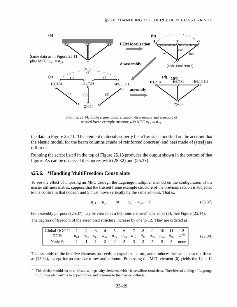
Figure 25.14. Finite element discretization, disassembly and assembly oftrussed frame example structure with MFC uy1 = uy5.
the data in Figure 25.11. The element material property list elemat is modified on the account thatthe elastic moduli for the beam columns (made of reinforced concrete) and bars made of (steel) aredifferent.
Running the script listed in the top of Figure 25.13 produces the output shown in the bottom of thatfigure. As can be observed this agrees with (25.32) and (25.33).
§25.6. *Handling MultiFreedom Constraints
To see the effect of imposing an MFC through the Lagrange multiplier method on the configuration of themaster stiffness matrix, suppose that the trussed frame example structure of the previous section is subjectedto the constraint that nodes 1 and 5 must move vertically by the same amount. That is,
uy1 = uy5 or uy1 − uy5 = 0. (25.37)
For assembly purposes (25.37) may be viewed as a fictitious element4 labeled as (6). See Figure (25.14).
The degrees of freedom of the assembled structure increase by one to 12. They are ordered as
Global DOF #: 1 2 3 4 5 6 7 8 9 10 11 12DOF: ux1 uy1 θz1 ux2 uy2 ux3 uy3 θz3 ux5 uy5 θz5 λ(6)
Node #: 1 1 1 2 2 3 3 3 5 5 5 none(25.38)
The assembly of the first five elements proceeds as explained before, and produces the same master stiffnessas (25.34), except for an extra zero row and column. Processing the MFC element (6) yields the 12 × 12
4 This device should not be confused with penalty elements, which have stiffness matrices. The effect of adding a “Lagrangemultiplier element” is to append rows and columns to the master stiffness.
25–19

Chapter 25: THE ASSEMBLY PROCESS
bordered stiffness
K =
175.6 −19.2 0 −25.6 19.2 −150. 0 0 0 0 0 0−19.2 36.9 45. 19.2 −14.4 0 −22.5 45. 0 0 0 1.
0 45. 120. 0 0 0 −45. 60. 0 0 0 0−25.6 19.2 0 51.2 0 0 0 0 −25.6 −19.2 0 0
19.2 −14.4 0 0 228.8 0 −200. 0 −19.2 −14.4 0 0−150. 0 0 0 0 300. 0 0 −150. 0 0 0
0 −22.5 −45. 0 −200. 0 245. 0 0 −22.5 45. 00 45. 60. 0 0 0 0 240. 0 −45. 60. 00 0 0 −25.6 −19.2 −150. 0 0 175.6 19.2 0 00 0 0 −19.2 −14.4 0 −22.5 −45. 19.2 36.9 −45. −1.
0 0 0 0 0 0 45. 60. 0 −45. 120. 00 1. 0 0 0 0 0 0 0 −1. 0 0
(25.39)
in which the coefficients 1 and −1 associated with the MFC (25.37) end up in the last row and column of K.
There are several ways to incorporate multiplier adjunction into an automatic assembly procedure. The mostelegant ones associate the fictitious element with a special freedom signature and a reserved position in theNFA. Being of advanced nature such schemes are beyond the scope of this Chapter.
Notes and Bibliography
The DSM assembly process for the simplest case of §25.3 is explained in any finite element text. Few textscover, however, the complications that arise in more general scenarios. Especially when VFCs are allowed.
Assembler implementation flavors have fluctuated since the DSM became widely accepted as standard. Variantshave been strongly influenced by limits on random access memory (RAM). Those limitations forced the useof “out-of-core” blocked equation solvers, meaning that heavy use was made of disk auxiliary storage to storeand retrieve the master stiffness matrix in blocks. Only a limited number of blocks could reside on RAM.Thus a straightforward element-by-element assembly loop (as in the assemblers presented here) was likely to“miss the target” on the receiving end of the merge, forcing blocks to be read in, modified and saved. On largeproblems this swapping was likely to “trash” the system with heavy I/O, bringing processing to a crawl.
One solution favored in programs of the 1965–85 period was to process all elements without assembling, savingmatrices on disk. The assembler then cycled over stiffness blocks and read in the contributing elements. Withsmart asynchronous buffering and tuned-up direct access I/O such schemes were able to achieved reasonableefficiency. However, system dependent logic quickly becomes a maintenance nightmare.
A second way out emerged by 1970: the frontal solvers referenced in Chapter 11. A frontal solver carries outassembly, BC application and solution concurrently. Element contributions are processed in a special orderthat traverses the FEM mesh as a “wavefront.” Application of displacement BCs and factorization can “trailthe wave” once no more elements are detected as contributing to a given equation. As can be expected oftrying to do too much at once, frontal solvers can be extremely sensitive to changes. One tiny alteration in theelement library over which the solver sits, and the whole thing may crumble like a house of cards.
The availability of large amounts of RAM (even on PCs and laptops) since the mid 90s, has had a happyconsequence: interweaved assembly and solver implementations, as well as convoluted matrix blocking, areno longer needed. The assembler can be modularly separated from the solver. As a result even the mostcomplex assembler presented here fits in one page of text. Of course it is too late for the large scale FEMcodes that got caught in the limited-RAM survival game decades ago. Changing their assemblers and solversincrementally is virtually impossible. The gurus that wrote those thousands of lines of spaghetti Fortran arelong gone. The only practical way out is rewrite the whole shebang from scratch. In a commercial environmentsuch investment-busting decisions are unlikely.
25–20

Exercises
Homework Exercises for Chapter 25
The Assembly Process
EXERCISE 25.1 [D:10] Suppose you want to add a six-node plane stress quadratic triangle to the METassembler of §25.4. Sketch how you would modify the module of Figure 25.6 for this to happen.
EXERCISE 25.2 [C:10] Exercise the module ElementFreedomTable listed in Figure 25.10 on the trussedframe structure. Verify that it produces the last column of (25.26).
EXERCISE 25.3 [D:15] Describe the logic of module ElementFreedomTable listed in Figure 25.10. Can itreturn zero entries in the EFT? If yes, give a specific example of how this can happen. Hint: read the Chaptercarefully.
EXERCISE 25.4 [A/C:30] The trussed frame structure of Figure 25.4 is reinforced with two triangular steelplates attached as shown in Figure ?(a). The plate thickness is 1.6 mm= 0.0016 m; the material is isotropicwith E = 240000 MPa and ν = 1/3. Each reinforcing plate is modeled with a single plane stress 3-nodelinear triangle. The triangles are numbered (6) and (7), as illustrated in Figure E25.1(c). Compute the masterstiffness matrix K of the structure.5
Plate
(6) (7)
Plate properties:E =240000 MPa, ν=1/3 h =1.6 mm = 0.0016 m,Other dimensions & propertiessame as in the trussed frame of Fig. 25.11
BarBar
Bar
1
1(1,2,3)1(1,2,3)
2
3(6,7,8)3(6,7,8)
5
5(9,10,11)5(9,10,11)
3
2(4,5) 2(4,5)
(a)
(b)
(c) (d)
disassembly
assembly
FEM idealization
(1) (2)
(3) (4) (5)
Beam-column Beam-column
(node 4:undefined)
x
y
x
y
Plate
Figure E25.1. Plate-reinforced trussed frame structure for Exercise 25.4.
This exercise may be done through Mathematica. For this download Notebook ExampleAssemblers.nb fromthis Chapter index, and complete Cell 4 by writing the assembler.6 The plate element identifier is "Trig3".The driver script to run the assembler is also provided in Cell 4 (blue text).
5 This structure would violate the compatibility requirements stated in Chapter 19 unless the beams are allowed to deflectlaterally independently of the plates. This is the fabrication actually sketched in Figure E25.1(a).
6 Cells 1–3 contain the assemblers presented in §25.3, §25.4 and §25.5, respectively, which may be used as guides. Thestiffness modules for the three element types used in this structure are available in Cells 2 and 3 and may be reused forthis Exercise.
25–21

Chapter 25: THE ASSEMBLY PROCESS
When reusing the assembler of Cell 3 as a guide, please do not remove the internal Print commands that showelement information (red text). Those come in handy for debugging. Please keep that printout in the returnedhomework to help the grader.
Another debugging hint: check that the master stiffness (25.32) is obtained if the plate thickness, called hplatein the driver script, is temporarily set to zero.
Target:
K =
337.6 −19.2 0 −25.6 91.2 −312. −72. 0 0 0 0−19.2 90.9 45. 91.2 −14.4 −72. −76.5 45. 0 0 0
0 45. 120. 0 0 0 −45. 60. 0 0 0−25.6 91.2 0 243.2 0 −192. 0 0 −25.6 −91.2 091.2 −14.4 0 0 804.8 0 −776. 0 −91.2 −14.4 0
−312. −72. 0 −192. 0 816. 0 0 −312. 72. 0−72. −76.5 −45. 0 −776. 0 929. 0 72. −76.5 45.
0 45. 60. 0 0 0 0 240. 0 −45. 60.
0 0 0 −25.6 −91.2 −312. 72. 0 337.6 19.2 00 0 0 −91.2 −14.4 72. −76.5 −45. 19.2 90.9 −45.
0 0 0 0 0 0 45. 60. 0 −45. 120.
(E25.1)
EXERCISE 25.5 [A:30] §25.5 does not explain how to construct the NFAT from the input data. (In the trussedframe example script, nodfat was set up by inspection, which is OK only for small problems.) Explain howthis table could be constructed automatically if the EFS of each element in the model is known. Note: thelogic is far from trivial.
25–22