THE ANTICAUSAL SOLUTIONS OF THE PARTIAL

DIFFERENTIAL OPERATOR ♢km AND ♢k

B,m RELATED TO THE

DIAMOND OPERATOR AND BESSEL-DIAMOND OPERATOR

MR. SUDPRATHAI BUPASIRI

SAKON NAKHON RAJABHAT UNIVERSITY

2014

THE ANTICAUSAL SOLUTIONS OF THE PARTIAL

DIFFERENTIAL OPERATOR ♢km AND ♢k

B,m RELATED TO THE

DIAMOND OPERATORR AND BESSEL-DIAMOND OPERATOR

MR. SUDPRATHAI BUPASIRI

SAKON NAKHON RAJABHAT UNIVERSITY

2014

TABLE OF CONTENTS

Page

CHAPTER I INTRODUCTION 1

CHAPTER II BASIC CONCEPTS AND PRELIMINARIES 6

2.1 Test functions 6

2.2 Distributions 9

2.3 Gamma functions 11

2.4 Properties of the convolution of distributions 12

2.5 causal (anticausal) distributions 13

CHAPTER III CAUSAL AND ANTICAUSAL SOLUTION OF THE

OPERATOR ♢km 15

3.1 Main results 15

REFERENCES 17

VITAE 19

RESEARCH PAPER: Causal and Anticausal Solution of the Operator ♢km 20

CHAPTER I

INTRODUCTION

Let x = (x1, x2, . . . , xn) be a point of the n - dimensional space Rn,

u = x21 + x22 + · · ·+ x2p − x2p+1 − x2p+2 − · · · − x2p+q, p+ q = n (1.1.1)

where p + q = n. Define Γ+ = {x ∈ Rn : x1 > 0 and u > 0} which designates

the interior of the forward cone and Γ+ designates its closure and the following

functions introduce by Nozaki ([16], p.72) that

Rα(u) =

uα−n2

Kn(α)if x ∈ Γ+

0 if x ∈ Γ+,(1.1.2)

Rα(u) is called the ultra-hyperbolic kernel of Marcel Riesz. Here α is a complex

parameter and n the dimension of the space. The constant Kn(α) is defined by

Kn(α) =π

n−12 Γ

(2+α−n

2

)Γ(1−α2

)Γ(α)

Γ(2+α−p

2

)Γ(p−α2

) (1.1.3)

and p is the number of positive terms of

u = x21 + x22 + · · ·+ x2p − x2p+1 − x2p+2 − · · · − x2p+q, p+ q = n

and let supp Rα(x) ⊂ Γ+. Now Rα(x) is an ordinary function if Re (α) ≥ n

and is a distribution of α if Re (α) < n.

Let x = (x1, . . . , xn) be a point of the n-dimensional Euclidean space Rn.

Consider a nondegenerate quadratic form in n variables of the form

P = P (x) = x21 + x22 + · · ·+ x2p − x2p+1 − x2p+2 − · · · − x2p+q, (1.1.4)

where p+ q = n. The distributions (P ± i0)λ are defined by

(P ± i0)λ = limε→0

{P ± iε|x|2}λ

where ε > 0, |x|2 = x21 + x22 + · · ·+ x2n, λ ∈ C.

2

Moreover the distribution (P ± i0)λ are analytic in λ every where except

at λ = −n2− k, k = 0, 1, . . . where they have simple poles.

Similarly, the distribution (m2 + P ± i0)λ is denote by

(m2 + P ± i0)λ = limε→0

{m2 + P ± iε|x|2}λ

where m is a real positive number. ([4], p.289)

Following Trione ([12], p.32) by causal (anticausal) distributions we mean

distributions of the form T (P ± i0, λ), P = P (x), T (P ± i0, λ) = (P ± i0)λf(P ±

i0, λ), f(z, λ) an entire function in the variables z, λ .

Let

Gα(P ± i0,m, n) = Hα(m,n)(P ± i0)12(α−n

2)K(n−α

2)(√m2(P ± i0)) (1.1.5)

where m is a real positive real number α ∈ C, Kν designates the modified Bessel

function of the third kind

Kν(z) =π

2

I−ν(z)− Iν(z)

secπν, Iν(z) =

∞∑m=0

( z2)2m+r

m!Γ(m+ ν + 1)

and

Hα(m,n) =2

1−(α+n)2 (m2)(

12)(α−n

2)e

π2qi

πn2Γ(α

2)

We introduce an auxiliary weight function

λα(P ± i0,m, n) = eiqπ2 2

1−(α+n)2 (m2)(

12)(α−n

2)(P ± i0)

(n+α)4 K (n+α)

2

√m2(P ± i0)

that is a causal (anticausal) analoque to the auxiliary weight function introduce

by Rubin ([2], p. 1247).

Let us define the n-dimensional ultrahyperbolic Klein-Gordon operator

iterated k-times

(�+m2)k =

[∂2

∂x21+ · · ·+ ∂2

∂x2p− ∂2

∂x2p+1

− · · · − ∂2

∂x2p+q

+m2

]k, where

� =

[∂2

∂x21+ · · ·+ ∂2

∂x2p− ∂2

∂x2p+1

− · · · − ∂2

∂x2p+q

]. (1.1.6)

3

The distributional function G2k(P ± i0,m, n) where n is an integer ≥ 2 and

k = 1, 2, 3, . . . are elementary causal (anticausal) solutions of the ultrahyperbolic

Klein-Gordon operator iterated k-times

(�+m2)kG2k(P ± i0,m, n) = δ.

Gelfand and Shilov [4] have first introduced the elementary solution of

the n-Dimensional Classical Diamond Operator, and have defined the distribu-

tion (P ± i0)λ as

(P ± i0)λ = limε→0

{P ± iε|x|2}λ

where ε > 0, |x|2 = x21 + x22 + · · · + x2n, λ ∈ C. The distributions (P ± i0)λ are

an important contribution of Gelfand and Shilov.

Moreover the distribution (P ± i0)λ are analytic in λ every where except

at λ = −n2− k, k = 0, 1, . . . where they have simple poles.

Kananthai [1] has studied the solution of n-dimensional diamond opera-

tor and the first introduce diamond operator, defined by

♢k =

[p∑

i=1

∂2

∂x2i

2

−p+q∑

j=p+1

∂2

∂x2j

2]k

(1.1.7)

, where p+q = n. Bupasiri [9] has studied the solution of n-dimensional operator

related to the diamond operator and defined by

♢k =

[1

c4

p∑i=1

∂2

∂x2i

2

−p+q∑

j=p+1

∂2

∂x2j

2]k

(1.1.8)

, where p+ q = n

The operator ♢k can be written as ♢k = △k�k = �k△k. Thus, the

operator ♢km can be factorized in the following form

♢km =

( p∑i=1

∂2

∂x2i+m2

2

)2

−

(p+q∑

j=p+1

∂2

∂x2j− m2

2

)2k

=

[p∑

i=1

∂2

∂x2i−

p+q∑j=p+1

∂2

∂x2j+m2

]k [ p∑i=1

∂2

∂x2i+

p+q∑j=p+1

∂2

∂x2j

]k(1.1.9)

4

, where p+q = n is the dimension of Rn, k is a nonnegative integer. The Laplace

operator and the ultra-hyperbolic Klein Gordon operator are defined by

△ =

p∑i=1

∂2

∂x2i+

p+q∑j=p+1

∂2

∂x2j(1.1.10)

and

�+m2 =

p∑i=1

∂2

∂x2i−

p+q∑j=p+1

∂2

∂x2j+m2 (1.1.11)

, where

� =

p∑i=1

∂2

∂x2i−

p+q∑j=p+1

∂2

∂x2j(1.1.12)

is the ultra-hyperbolic operator. Thus, equation (1.1.9) can be written as

♢km = △k(�+m2)k = (�+m2)k △k . (1.1.13)

In 1988, Trione [10] studied the elementary solution of the ultra-hyperbolic

Klein Gordon operator, which iterated k-times, and is defined by

(�+m2)k =

[p∑

i=1

∂2

∂x2i−

p+q∑j=p+1

∂2

∂x2j+m2

]k. (1.1.14)

We obtain the elementary solution W2k(P ± i0,m), defined by

W2k(P ± i0,m) =∞∑r=0

(−kr

)(m2)rR2k+2r(P ± i0), (1.1.15)

where R2k+2r(P ± i0) is defined by (1.1.18).

Therefore, W2k(P ± i0,m) is the unique elementary retarded (P ± i0)λ-

ultrahyperbolic solution of the Klein-Gordon operator, iterated k -times. That

is

(�+m2)kW2k(P ± i0,m) = (�+m2)k(�+m2)−kδ = δ (1.1.16)

Putting k = 1 , the formula (1.1.15) says that W2(P ± i0,m) is the unique

elementary retarded (P ± i0)λ-ultrahyperbolic solution of the Klein-Gordon op-

erator

Now, the purpose of this work is to find the elementary solution of the

operator ♢km, that is

♢km(P ± i0) = δ,

5

where (P ± i0) is the elementary solution, δ is the Dirac-delta distribution, k is

a nonnegative integer and x = (x1, . . . , xn) ∈ Rn.

Let x = (x1, x2, . . . , xn) be a point of the n - dimensional space Rn,

P = P (x) = x21 + x22 + · · ·+ x2p − x2p+1 − x2p+2 − · · · − x2p+q, (1.1.17)

where p + q = n. Define Γ+ = {x ∈ Rn : x1 > 0 and P > 0} which designates

the interior of the forward cone and Γ+ designates its closure and the following

functions introduce by Nozaki ([16], p.72) that

Rα = Rα(P ± i0) =

(P±i0)

α−n2

Kn(α)if x ∈ Γ+

0 if x ∈ Γ+,(1.1.18)

Rα is called the ultra-hyperbolic kernel of Marcel Riesz. Here α is a complex

parameter and n the dimension of the space. The constant Kn(α) is defined by

Kn(α) =π

n−12 Γ2+α−n

2Γ1−α

2Γ(α)

Γ2+α−p2

Γp−α2

(1.1.19)

and p is the number of positive terms of

P = P (x) = x21+x22+ · · ·+x2p−x2p+1−x2p+2−· · ·−x2p+q, p+q = n (1.1.20)

and let supp Rα(P ± i0) ⊂ Γ+. Now Rα is an ordinary function if Re (α) ≥ n

and is a distribution of α if Re (α) < n.

Now, we define the causal (anticausal) distributions Sα(P′±i0) as follows:

Sα = Sα(P′ ± i0)

eiπα2 e±

i π2 q

2 Γ(n−α2)

2απn2Γ(α

2)

(P ′ ± i0)α−n2 (1.1.21)

where α ∈ C,

P ′ = P ′(x) = x21 − x22 − · · · − x2n

and q is the number of negative terms of the quadratic form P . The

distributional functions Sα are the causal (anticausal) analogues of the elliptic

kernel of M. Riesz ([7], pp.16-21), and have analogous properties [13].

CHAPTER II

BASIC CONCEPTS AND PRELIMINARIES

In this chapter, we studied some properties of the test function, the dis-

tribution, the gamma function , Causal and anticausal Solution of the Operator

♢km which will be used in later chapters.

2.1 Test functions

Let Rn be a real n-dimensional space in which we have a Cartesian system

of coordinates such that a point P is denoted by x = (x1, x2, . . . , xn) and the

distance r, of P from the origin, is r = |x| = (x21 + x22 + · · · + x2n)1/2. Let k be

an n-tuple of nonnegative integer, k = (k1, k2, . . . , kn), the so-called multiindex

of order n; then we define

|k| = k1 + k2 + · · ·+ kn, xk = xk11 xk22 · · · xknn

and

Dk =∂|k|

∂xk11 ∂xk22 · · · ∂xknn

=∂k1+k2+···+kn

∂xk11 ∂xk22 · · · ∂xknn

= Dk11 D

k22 · · ·Dkn

n ,

where Dj = ∂/∂xj, j = 1, 2, . . . , n. For the one-dimensional case, Dk reduces

to d/dx. Furthermore, if any component of k is zero, the differentiation with

respect to the corresponding variable is omitted.

Example 2.1.1. In R3, with k = (3, 0, 4), we have

Dk = ∂7/∂x31∂x43 = D3

1D43.

Definition 2.1.2. A function f(x) is locally integrable in Rn if∫R|f(x)|dx exists

for every bounded region R in Rn. A function f(x) is locally integrable on a

hypersurface in Rn if∫S|f(x)|dS exists for every bounded region S in Rn−1.

7

Definition 2.1.3. The support of a function f(x) is the closure of the set of all

points x such that f(x) = 0. We shall denote the support of f by supp f .

Example 2.1.4. For f(x) = sin x, x ∈ R, the support of f(x) consists of the

whole real line, even though sin x vanishes at x = nπ.

Definition 2.1.5. ([6]). If supp f is a bounded set, then f is said to have a

compact support.

We have observed that an operational quantity such as δ(x) becomes

meaningful if it is first multiplied by a sufficiently smooth auxiliary function

and then integrated over the entire space. This point of view is also taken as

the basis for the definition of an arbitrary generalized function. Accordingly,

consider the spaceD consisting of real-valued functions ϕ(x) = ϕ(x1, x2, . . . , xn),

such that the following hold:

(1) ϕ(x) is an infinitely differentiable function defined at every point of Rn.

This means that Dkϕ exists for all multiindices k. Such a function is also

called a C∞ function.

(2) There exists a number A such that ϕ(x) vanishes for r > A. This means

that ϕ(x) has a compact support. Then ϕ(x) is called a test function.

Example 2.1.6. The support of the function

f(x) =

0, for −∞ < x ≤ −1

x+ 1, for −1 < x < 0

1− x, for 0 ≤ x < 1

0, for 1 ≤ x <∞

is [−1, 1], which is compact.

Example 2.1.7. The prototype of a test function belonging to D is

ϕ(x, a) =

exp(− a2

a2−r2

), for r < a

0, for r > a.

(2.1.1)

Its support is clearly r ≤ a.

8

The following properties of the test functions are evident.

(1) If ϕ1 and ϕ2 are in D, then so is c1ϕ1 + c2ϕ2, where c1 and c2 are real

numbers. Thus D is a linear space.

(2) If ϕ ∈ D, then so is Dkϕ .

(3) For a C∞ function f(x) and ϕ ∈ D, fϕ ∈ D.

(4) If ϕ(x1, x2, . . . , xm) is anm-dimensional test function and ψ(xm+1, xm+2, . . . , xn)

is an (n−m) -dimensional test function, then ϕψ is an n-dimensional test

function in the variables x1, x2, . . . , xn.

Definition 2.1.8. The Schwartz space or space of rapidly decreasing functions

S on Rn is the function space

S(Rn) = { f ∈ C∞(Rn) | ∥f∥α,β <∞∀α, β },

where α, β are multi-indices, C∞(Rn) is the set of smooth functions from Rn to

C, and

∥f∥α,β = ∥xαDβf∥∞.

Here, ∥ · ∥∞ is the supremum norm, and we use multi-index notation.

Example 2.1.9. If i is a multi-index, and is a positive real number, then

xie−ax2 ∈ S(R).

Any smooth function f with compact support is in S. This is clear since any

derivative of f is continuous, so (xαDβ)f has a maximum in Rn.

Definition 2.1.10. A sequence {ϕm},m = 1, 2, . . . , where ϕm ∈ D, converges

to ϕ0 if the following two conditions are satisfied:

(1) All ϕm as well as ϕ0 vanish outside a common region.

(2) Dkϕm → Dkϕ0 uniformly over Rn as m→ ∞ for all multiindices k.

It is not difficult to show that ϕ0 ∈ D and hence that D is closed (or is complete)

with respect to this definition of convergence. For the special case ϕ0 = 0, the

sequence {ϕm} is called a null sequence.

9

Example 2.1.11. The sequence

{(1/m)ϕ(x, a)}, (2.1.2)

where ϕ(x, a) is defined by (2.1.1), is a null sequence. However, the sequence

(1/m)ϕ(x/m, a) is not a convergent sequence, because the support of the func-

tion ϕ(x/m, a) is the sphere with radius ma, which is unique for each m.

In addition to the space D of test functions, we shall use certain sub-

spaces of D. For a region R in Rn, the space DR contains those test functions

whose support lies in R, that is,

DR ≡ {ϕ : ϕ ∈ D, supp ϕ ⊂ R}. (2.1.3)

It is clearly a linear subspace of D.

Example 2.1.12. Dx and Dy are two one-dimensional subspaces of test func-

tions ϕ(x) and ϕ(y) and are contained inDxy, which is the space of test functions

ϕ(x, y) in R2. The convergence in DR is defined in the same manner as that in

the space D.

2.2 Distributions

Definition 2.2.1. A linear functional t on the space D of test functions is

an operation (or a rule) by which we assign to every test function ϕ(x) a real

number denoted ⟨t, ϕ⟩, such that

⟨t, c1ϕ1 + c2ϕ2⟩ = c1 ⟨t, ϕ1⟩+ c2 ⟨t, ϕ2⟩ (2.2.1)

for arbitrary test functions ϕ1 and ϕ2 and real numbers c1 and c2.

Definition 2.2.2. A linear functional on D is continuous if and only if the se-

quence of numbers ⟨t, ϕm⟩ converges to ⟨t, ϕ⟩ when the sequence of test functions

{ϕm} converges to the test function ϕ. Thus

limm→∞

⟨t, ϕm⟩ =⟨t, lim

m→∞ϕm

⟩.

10

In physical problems, one often encounters idealized concepts such as a

force concentrated at a point ξ or an impulsive force that acts instantaneously.

These forces are described by the Dirac-delta function δ(x−ξ), which has several

significant properties:

δ(x− ξ) = 0, x = ξ, (2.2.2)∫ b

a

δ(x− ξ)dx =

0, for a, b < ξ or ξ < a, b

1, for a ≤ ξ ≤ b,

(2.2.3)

and ∫ ∞

−∞δ(x− ξ)dx = 1. (2.2.4)

Equation (2.2.4) is a special case of the general formula∫ ∞

−∞δ(x− ξ)f(x)dx = f(ξ), (2.2.5)

where f(x) is a sufficiently smooth function. Relation (2.2.5) is called the sifting

property or the reproducing property of the delta function, and (2.2.4) is obtained

from it by putting f(x) = 1.

We now have all the tools for defining the concept of distributions.

Definition 2.2.3. A continuous linear functional on the space D of test func-

tions is called a distribution.

Example 2.2.4. The Heaviside distribution in Rn is ⟨HR, ϕ⟩ =∫Rϕ(x)dx,

where

HR(x) =

1 for x ∈ R

0 for x ∈ R.

(2.2.6)

For R, (2.2.6) becomes

⟨H,ϕ⟩ =∫ ∞

0

ϕ(x)dx. (2.2.7)

Example 2.2.5. The Dirac delta distribution in Rn is

⟨δ(x− ξ), ϕ(x)⟩ = ϕ(ξ) (2.2.8)

for ξ is a fixed point in Rn. Linearity of this functional follows from the relation

⟨δ, c1ϕ1(x) + c2ϕ2(x)⟩ = c1ϕ1(ξ) + c2ϕ2(ξ) = c1 ⟨δ, ϕ1⟩+ c2 ⟨δ, ϕ2⟩ , (2.2.9)

where c1 and c2 are arbitrary real constants.

11

Definition 2.2.6. A distribution E is said to be an elementary solution for the

differential operator L if

LE = δ.

Example 2.2.7. The function R2k(u) is the elementary solution of the operator

�k, where �k is defined by (1.1.6) and R2k(u) is defined by (1.1.18) with α = 2k.

That is, �kR2k(u) = δ , see([5], p.147)

2.3 Gamma functions

Definition 2.3.1. The gamma function is denoted by Γ and is defined by

Γ(z) =

∫ ∞

0

e−ttz−1dt, (2.3.1)

where z is a complex number with Re z > 0

Example 2.3.2. Show that Γ(1) = 1.

Proof. By definition 2.3.1, we obtain

Γ(1) =

∫ ∞

0

e−tdt

= lima→∞

(−e−t|a0)

= 1.

�

Proposition 2.3.3. ([3]) Let z be a complex number. Then

(1) zΓ(z) = Γ(z + 1), z = 0,−1,−2, . . .

(2) Γ(z)Γ(1− z) =π

sinπz, z = 0,±1,±2, . . .

(2) Γ(z)Γ(z + 1

2

)= 21−2z

√πΓ(2z), z = 0,−1,−2, . . .

12

2.4 Properties of the convolution of distribution

Definition 2.4.1. The convolution f ∗ g of two functions f(t) and g(t), both

in Rn, is defined as

f ∗ g =∫ ∞

−∞f(τ)g(t− τ)dτ. (2.4.1)

Example 2.4.2. Let

f(t) =

l−t, for t ≥ 0

0, for t ≥ 0

and

g(t) =

sin t, for 0 ≤ t ≤ π2

0, otherwise.

Since

f ∗ g =∫ ∞

−∞f(τ)g(t− τ)dτ,

f ∗ g =

∫ t

0l−t sin(t− τ)dτ, for 0 < t < π

2∫ t

t−π2l−t sin(t− τ)dτ, for t ≥ π

2

0, for t < 0.

Properties of the Convolution of Distributions

Property 1. Commutativity.

s ∗ t = t ∗ s (2.4.2)

Property 2. Associativity.

(s ∗ t) ∗ u = s ∗ (t ∗ u) (2.4.3)

if the supports of the two of these three distributions are bounded or if the

supports of all three distributions are bounded on the same side.

Proposition 2.4.3. ([6]). If the convolution s ∗ t exists, then the convolutions

(Dks) ∗ t and s ∗ (Dkt) exist, and

(Dks) ∗ t = Dk(s ∗ t) = s ∗ (Dkt). (2.4.4)

If L is a differential operator with constant coefficients, we find from (2.4.4)

that

(Ls) ∗ t = L(s ∗ t) = s ∗ (Lt). (2.4.5)

13

2.5 Causal (anticausal) distributions

Let x = (x1, . . . , xn) be a point of the n-dimensional Euclidean space Rn.

Consider a nondegenerate quadratic form in n variables of the form

P = P (x) = x21 + x22 + · · ·+ x2p − x2p+1 − x2p+2 − · · · − x2p+q, (2.5.1)

where p+ q = n. The distributions (P ± i0)λ are defined by

(P ± i0)λ = limε→0

{P ± iε|x|2}λ

where ε > 0, |x|2 = x21 + x22 + · · ·+ x2n, λ ∈ C.

Moreover the distribution (P ± i0)λ are analytic in λ every where except

at λ = −n2− k, k = 0, 1, . . . where they have simple poles. Similarly, the

distribution (m2 + P ± i0)λ is denote by

(m2 + P ± i0)λ = limε→0

{m2 + P ± iε|x|2}λ

where m is a real positive number. ([4], p.289)

Following Trione ([12], p.32) by causal (anticausal) distributions we mean

distributions of the form T (P ± i0, λ), P = P (x), T (P ± i0, λ) = (P ± i0)λf(P ±

i0, λ), f(z, λ) an entire function in the variables z, λ .

Let

Gα(P ± i0,m, n) = Hα(m,n)(P ± i0)12(α−n

2)K(n−α

2)(√m2(P ± i0)) (2.5.2)

where m is a real positive real number α ∈ C, Kν designates the modified Bessel

function of the third kind

Kν(z) =π

2

I−ν(z)− Iν(z)

secπν, Iν(z) =

∞∑m=0

( z2)2m+r

m!Γ(m+ ν + 1)

and

Hα(m,n) =2

1−(α+n)2 (m2)(

12)(α−n

2)e

π2qi

πn2Γ(α

2)

We introduce an auxiliary weight function

λα(P ± i0,m, n) = eiqπ2 2

1−(α+n)2 (m2)(

12)(α−n

2)(P ± i0)

(n+α)4 K (n+α)

2

√m2(P ± i0)

14

that is a causal (anticausal) analoque to the auxiliary weight function introduce

by Rubin ([2], p. 1247).

Let us define the n-dimensional ultrahyperbolic Klein-Gordon operator

iterated k-times

(�+m2)k =

[∂2

∂x21+ · · ·+ ∂2

∂x2p− ∂2

∂x2p+1

− · · · − ∂2

∂x2p+q

]k, The distributional function G2k(P ± i0,m, n) where n is an integer ≥ 2 and

k = 1, 2, 3, . . . are elementary causal (anticausal) solutions of the ultrahyperbolic

Klein-Gordon operator iterated k-times

(�+m2)kG2k(P ± i0,m, n) = δ.

CHAPTER III

CAUSAL AND ANTICAUSAL SOLUTION OF THE

OPERATOR ♢km

In this chapter, we study the causal and anticausal solution of the oper-

ator ♢km. Moreover, such a solution is unique.

3.1 Main results

Lemma 3.1.1. Sα and Wβ are tempered distributions.

Proof. By following Kananthai ([1], p.31), we know that Donoghue ([15],

pp.154-155) establishes that every homogeneous distribution is a tempered dis-

tribution and see [11].

Lemma 3.1.2. The distributions S2k = S2k(P′ ± i0, n), 2k = n + 2r , r =

0, 1, . . . , are the causal (anticausal) elementary solutions of the homogeneous

ultrahyperbolic operator iterated k -times; equivalently, the following formula is

valid

�kS2k(P′ ± i0, n) = δ (3.1.1)

here �k is defined by (1.1.12) and S2k(P′ ± i0, n) by the formula (1.1.21).

The proof of this Lemma is given in [14].

Theorem 3.1.3. The convolution distributional functions

(−1)kS2k(P′ ± i0) ∗W2k(P ± i0,m), (3.1.2)

which are defined by (1.1.21) and (1.1.15), respectively, where k = 1, 2, . . . , n

integer ≥ 2; are the elementary solution of the ♢km(P ± i0) = δ, where ♢k

m is

the causal (anticausal) of the operator related to the diamond operator iterated

k-times defined by (1.1.9):

♢km(P ± i0) = δ. (3.1.3)

16

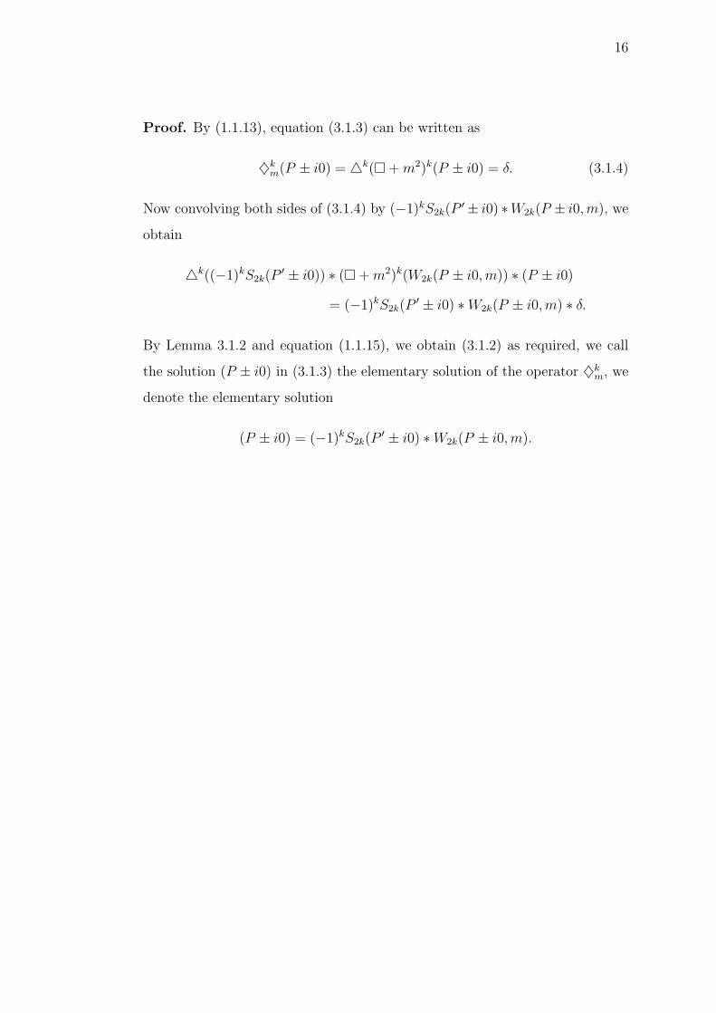
Proof. By (1.1.13), equation (3.1.3) can be written as

♢km(P ± i0) = △k(�+m2)k(P ± i0) = δ. (3.1.4)

Now convolving both sides of (3.1.4) by (−1)kS2k(P′ ± i0) ∗W2k(P ± i0,m), we

obtain

△k((−1)kS2k(P′ ± i0)) ∗ (�+m2)k(W2k(P ± i0,m)) ∗ (P ± i0)

= (−1)kS2k(P′ ± i0) ∗W2k(P ± i0,m) ∗ δ.

By Lemma 3.1.2 and equation (1.1.15), we obtain (3.1.2) as required, we call

the solution (P ± i0) in (3.1.3) the elementary solution of the operator ♢km, we

denote the elementary solution

(P ± i0) = (−1)kS2k(P′ ± i0) ∗W2k(P ± i0,m).

REFERENCES

[1] A. Kananthai. On the solutions of the n-dimensional diamond operator.

Appl. Math. Comput. 1997; 88: 27-37.

[2] B.S. Rubin. Description and inversion of Bessel potentials by us-

ing hypersingular integrals with weighted differences.Differential

Equation. 1986; 22: 10.

[3] H. Bateman. Higher transcendental function. Manuscript Project,

Vol. 1, New York: Mc-Graw Hill; 1953.

[4] I. M. Gelfand, and G. E. Shilov. Generalized functions. New York:

Academic Press; 1964.

[5] M. A. Tellez. The distribution Hankel transform of Marcel Riesz’s

ultra-hyperbolic kernel. Studied in Applied Mathematics, Massachusetts

Institute of Technology, Elsevier Science Inc. 1994; 93: 133-162.

[6] P. K. Ram. Generalized functions theory and technique. 2nd ed.,

Birkhauser Boston: Hamilton Printing; 1998.

[7] Riesz, M., L’integrale de Riemann-Liouville et le probleme de

Cauchy. Acta Mathematica, (81)(1949),1-223.

[8] S. Bupasiri and K. Nonlaopon. On the weak solution of the compound

equation related to the ultra-hyperbolic operator. Far East Journal of

Applied Mathematics 2009; 35(1): 129-139.

[9] S. Bupasiri, On the solution of the n-dimensional operator related to the

diamond operator, FJMS. (45)(2010), 69-80.

[10] S.E. Trione., On the elementary retarded ultra-hyperbolic solution of the

Klein-Gordon operator, iterated k-times. Studies in Applied Mathematics,(79)21-

141.

18

[11] S.E. Trione., On the elementary (P ± i0)λ- ultra-hyperbolic solution of

the Klein-Gordon operator, iterated k-times. Integral Transforms and

Special Functions, an International Journal. Prudnikov, A.P. (Ed.),

(9)(2)49-162.

[12] S.E. Trione. Distributional products. In Cursos de Matematica. No.

3. Instituto Argentino de Matematica. C.O.N.I.C.E.T.; 1965.

[13] Trione, S.E., Distributional product. Cursos de Matematica, IAM-CONICET,

Buenos Aires, 3, 1980.

[14] Trione, S.E., On the solutions of the causal and anticausal n-dimensional

diamond operator, Integral Transform and Special Functions, (13)(2002),49-

57.

[15] W. F. Donoghue. Distribution and Fourier transform. New York:

Academic Press; 1969.

[16] Y. Nozaki. On Riemann - Liouville integral of ultra - hyperbolic type.

Kodai Mathematical Seminar Reports 1964; 6(2): 69 - 87.

VITAE

Name Mr. Sudprathai Bupasiri

Date of birth January 23, 1981

Place of birth Nakhon Phanom Province, Thailand

Institution Attended Mattayom 6 in Akatumnuaysuksa

School in 1999, Sakon Nakhon, Thailand.

Bachelor of Education (Mathematics)

from Rajabhat Institute Sakon Nakhon

in 2003, Thailand.

And enrolled in Master of Science Program in

Mathematics, Khon Kaen University in 2007.

CHAPTER II

BASIC CONCEPTS AND PRELIMINARIES

In this chapter, we studied some properties of the test function, the dis-

tribution, the gamma function , Causal and anticausal Solution of the Operator

♢km which will be used in later chapters.

2.1 Causal and anticausal Solution of the Operator ♢km