The Ancient Origins of Cross-CountryHeterogeneity in Risk Preferences∗

Anke Becker Benjamin Enke Armin Falk

May 6, 2015

Abstract

Using novel representative preference data on 80,000 individuals from 76countries, this paper shows that the migratory movements of our early ances-tors thousands of years ago have left a footprint in the contemporary cross-country distribution of risk preferences. Across a wide range of regressionspecifications, differences in risk aversion between populations are significantlyincreasing in the length of time elapsed since the respective groups shared com-mon ancestors. This result obtains for various proxies for the structure andtiming of historical population breakups, including genetic and linguistic dataor predicted measures of migratory distance. In addition, we provide evidencethat the within-country heterogeneity in risk aversion significantly decreases inmigratory distance from the geographical origin of mankind. Taken together,our results point to the importance of very long-run events for understandingthe global distribution of one of the key economic traits.

JEL classification: D01, D03Keywords : Risk preferences, out of Africa, persistence, genetic distance, geneticdiversity

∗We are grateful to Quamrul Ashraf, Klaus Desmet, Nathan Nunn, Uwe Sunde, Hans-JoachimVoth, and Romain Wacziarg for very helpful discussions. Valuable comments were also receivedfrom seminar audiences at Bonn, Munich, the NBER Economics of Culture and Institutions Meeting2014, SITE Stanford 2014, the North-American ESA conference 2014, and the Annual Congress ofthe EEA 2013. We thank Quamrul Ashraf, Oded Galor, and Ömer Özak for generous data sharing.Ammar Mahran provided oustanding research assistance. Armin Falk acknowledges financial sup-port from the European Research Council through ERC # 209214. Becker, Enke, Falk: Universityof Bonn, Department of Economics, Adenauerallee 24-42, 53113 Bonn, Germany. anke.becker@uni-bonn.de, benjamin.enke@uni-bonn.de, armin.falk@uni-bonn.de

1 Introduction

Preferences over risk have been shown to vary substantially within populations andto predict a plethora of individual-level economic decisions. However, do risk prefer-ences also vary across countries? And if so, what explains this variation, i.e., whatare the ultimate determinants of heterogeneity in preferences? Using a novel, glob-ally representative data set on risk preferences, this paper seeks to provide an answerto these questions. Our key contribution is to show that the structure of mankind’sancient migration out of Africa and around the globe has had a persistent impact onthe between-country distribution of risk attitudes as of today. In light of the rele-vance of risk preferences in predicting important economic and social outcomes, theseresults contribute to understanding the ultimate sources of cross-country economicheterogeneity. Moreover, our findings add to the emerging literature on endogenouspreferences (Fehr and Hoff, 2011) in highlighting historical roots as a key driver inshaping preferences.

According to the widely accepted “Out of Africa hypothesis”, starting around50,000 years ago, early mankind migrated out of East Africa and continued to ex-plore and populate our planet through a series of successive migratory steps. Eachof these steps consisted of some sub-population breaking apart from the previouscolony and moving on to found new settlements. This pattern implies that somecontemporary population pairs have spent a longer time of human history apartfrom each other than others. As a result, the time elapsed since two groups sharedcommon ancestors differs across today’s population pairs. The key idea underlyingour analysis is that these differential time frames of separation have affected thecross-country distribution of risk preferences. First, populations that have spent along time apart from each other were exposed to differential historical experiences,which could affect preferences over risk (Callen et al., 2014). Second, due to, e.g.,random genetic drift, long periods of separation lead to different population-levelgenetic endowments, which might in turn shape risk attitudes.1 Both of these chan-nels imply that populations that have been separated for a long time in the courseof human history, should also exhibit different risk attitudes. Thus, we hypothesizethat the (absolute) difference in risk attitudes between countries reflects the lengthof separation of the respective populations, as evoked by the successive populationbreakups in ancient times.

To investigate this hypothesis, we use a novel dataset on risk preferences acrosscountries in combination with proxies for long-run human migration. As part of theGlobal Preference Survey (GPS), we collected two survey measures of risk preferences

1Cesarini et al. (2009) use a twin study to provide evidence for a genetic effect on risk preferences.

1

(see Falk et al., 2015a). The sample of 80,000 people from 76 countries is constructedto provide representative population samples within each country and geographicalrepresentativeness in terms of countries covered. The survey items – one qualitativeand one quantitative lottery-type measure of risk preferences – were selected andtested through a rigorous ex ante experimental validation procedure involving realmonetary stakes. The elicitation followed a standardized protocol that was imple-mented through the professional infrastructure of the Gallup World Poll. These dataallow the computation of a nationally representative level of risk aversion, and hencethe derivation of the absolute difference in risk attitudes within a country pair.2

We combine these data with three classes of proxies for the temporal patterns ofancient population fissions, i.e., proxies for the length of time since two populationsshared common ancestors. (i) First, we employ the FST and Nei genetic distancesbetween populations, as originally measured by the population geneticists Cavalli-Sforza et al. (1994) and introduced into the economics literature by Spolaore andWacziarg (2009). As population geneticists have long noted, whenever two pop-ulations split apart from each other in order to found separate settlements, theirgenetic distance increases over time due to random genetic drift. Thus, the geneticdistance between two populations is a measure of temporal distance since separation.(ii) Second, we use measures of predicted migratory distance between contemporarypopulations, which were constructed by Ashraf and Galor (2013b) and Özak (2010),respectively. The predicted migratory distance variable of Ashraf and Galor (2013b)is based on a procedure which exploits information on the geographic patterns ofearly migratory movements and constitutes a proxy for the predicted length of sep-aration of two populations.3 The human-mobility-index measure of Özak (2010), onthe other hand, explicitly computes the walking time between two countries’ cap-itals, taking into account topographic, climatic, and terrain conditions, as well ashuman biological abilities. (iii) Finally, we make use of the observation that linguis-tic trees closely follow the structure of separation of human populations and employa measure of linguistic distance between two populations as explanatory variable.In sum, we use various independent sources of data which are known to reflect thelength of separation of populations. Using these measures, we test the hypothesisthat the heterogeneity in risk preferences across contemporary populations is drivenby migratory movements in the distant past.

Our empirical analysis of the relationship between risk preferences and ancient

2Vieider et al. (2012) and Rieger et al. (2014) also collect data on the prevalence of risk attitudesin multiple countries. Their samples cover a much smaller set of countries and contain universitystudents, rendering conclusions about population-level differences in risk attitudes difficult.

3See Ramachandran et al. (2005).

2

migration patterns starts by establishing that the absolute difference in average riskattitudes between two countries is significantly increasing in the length of time sincetoday’s populations shared common ancestors, as proxied for by (observed) geneticdistance, predicted migratory distance, and linguistic distance. In a second step,using observed genetic distance as main measure, we investigate to what extentour main result is likely to be driven by contemporary environmental conditions, i.e.,omitted variables. We establish that the relationship between differences in risk pref-erences and length of separation is robust to an extensive set of covariates, includingcontrols for differences in the countries’ demographic composition, their geographicposition, prevailing climatic and agricultural conditions, institutions, and economicdevelopment. In all of the corresponding regressions, the point estimate is ratherstable, suggesting that unobserved heterogeneity is unlikely to drive our results, ei-ther (Altonji et al., 2005). Our result also holds when we exclude entire continents orobservations with large genetic distances from the analysis. Final robustness checksreveal that we obtain similar results when we use alternative genetic distance dataor the predicted migratory distance variables in the conditional regressions.

In sum, irrespective of the measure used, our results indicate the existence of arelationship between cross-country differences in risk attitudes and the pattern ofvery distant migratory movements, which is not explained by differences in the con-temporary environments people reside in. However, as established by the so-calledserial-founder effect of population genetics, the structure of successive populationbreakups also affects within-population diversity. Intuitively, due to the loss of het-erogeneity that is implied by small founder populations breaking apart from previousparental colonies, the diversity of a population decreases along migratory paths. Toinvestigate whether such a mechanism also plays out for preferences over risk, werelate the within-country standard deviation in risk preferences to a population’s(predicted) migratory distance from East Africa. The results show that, for bothpredicted migratory distance variables, the degree of the within-country heterogene-ity in individual risk attitudes is indeed significantly decreasing in migratory dis-tance from East Africa, and is hence positively correlated with the diversity of therespective genetic pool. Thus, along two major dimensions (means and variances),temporally very distant population fissions explain a significant fraction of today’scross-country heterogeneity in one of the key economic traits.

A number of recent contributions argue that the (cultural) diversity caused bylong-run migration thousands of years ago can have real aggregate economic effects.Spolaore and Wacziarg (2009, 2011) find a strong relationship between genetic dis-tance and income differences across countries and argue that lower cultural distance

3

between two countries facilitates the diffusion of knowledge.4 Ashraf and Galor(2013b) and Ashraf et al. (2014) document an inverted U-form relationship betweenper capita income and genetic diversity (migratory distance from East Africa). Theyargue that this pattern reflects the trade-off between more innovation and lower trustand cooperation that is associated with higher cultural diversity.5 Our paper nicelydovetails with this set of contributions as it shows that the genetic variables whichproxy for migratory flows indeed capture variation in an economically importanttrait (either between or within countries), as is implicitly or explicitly assumed bythese papers.

This paper also forms part of an active recent literature on the historical, biolog-ical, and cultural origins of beliefs and preferences. For example, Chen (2013) andGalor and Özak (2014) show that cross-country differences in future-orientation areaffected by a structural feature of languages and historical agricultural productivity.Tabellini (2008) and an earlier version of Guiso et al. (2009) relate interpersonal trustto linguistic features and the genetic distance between two populations. Nunn andWantchekon (2011), Voigtländer and Voth (2012) and Alesina et al. (2013) establishthe deep roots of trust, beliefs over the appropriate role of women in society, andanti-semitism.6 Desmet et al. (2011) show that, within Europe, genetic distance cor-relates with opinions and attitudes as expressed in the World Values Survey. Desmetet al. (2014) investigate the relationship between cultural traits and ethnicity. How-ever, presumably given the previous lack of data, this paper is the first contributionto study the origins of cross-country variation in risk preferences.

The remainder of this paper proceeds as follows. In the next section, we developour hypotheses on the relationship between the structure of migratory movementsand risk preferences, while Section 3 presents the data. Section 4 discusses our mainresult on the connection between differences in average risk attitudes and length ofseparation. In Section 5, we examine the within-country heterogeneity in risk prefer-ences. Section 6 concludes the paper by discussing correlations between country-levelrisk attitudes and economic, institutional, and health outcomes.

4Spolaore and Wacziarg (2014) find a negative relationship between genetic distance and theoccurrence of conflict. Gorodnichenko and Roland (2010) argue that genetic distance to the UnitedStates can be used as an instrument for the cultural “individualism” dimension to show a causaleffect on GDP. Proto and Oswald (2014) investigate the correlation between genetic distance toDenmark and happiness. Giuliano et al. (2014) show that the negative correlation between geneticdistance and bilateral trade vanishes once transportation costs are accounted for.

5Arbatli et al. (2013) and Ashraf and Galor (2013a) show that genetic diversity is related toethnolinguistic diversity and the emergence of civil conflicts.

6See also Guiso et al. (2006) and Fernández and Fogli (2006, 2009).

4

2 Risk Attitudes and the Great Human Expansion

According to the widely accepted theory of the origins and the dispersal of earlyhumans, the single cradle of mankind is to be found in East or South Africa andcan be dated back to roughly 100’000 years ago (see, e.g., Henn et al. (2012) for anoverview). Starting from East Africa, a small sample of hunters and gatherers exitedthe African continent around 50’000-60’000 years ago and thereby started what isnow also referred to as the “great human expansion”. This expansion continuedthroughout Europe, Asia, Oceania, and the Americas, so that mankind eventuallycame to settle on all continents. A noteworthy feature of this very long-run processis that it occurred through a large number of discrete steps, each of which consistedof a sub-sample of the original population breaking apart and leaving the previouslocation to move on and found new settlements elsewhere (so-called serial foundereffect). The main argument of this paper is that the pattern of successive breakupsaffected the distribution of risk preferences we observe around the globe today.

First, the series of migratory steps implied a frequent breakup of formerly unitedpopulations. After splitting apart, these sub-populations often settled geographicallydistant from each other, i.e., lived in separation. There are two channels throughwhich the length of separation of two groups might have had an impact on between-group differences in risk attitudes:

First, the fact that two populations have spent a long time apart from each otherimplies that they were subject to many differential historical experiences. Recentwork by, e.g., Callen et al. (2014) highlights that risk preferences are malleable byidiosyncratic experiences or, more generally, by the composition of people’s socialenvironment. Thus, the differential historical experiences which have accumulatedover thousands of years of separation might have given rise to differential attitudestowards risk as of today.

Second, whenever two populations spend time apart from each other, they developdifferent population-level genetic pools due to, e.g., random genetic drift. Given thatrisk attitudes are transmitted across generations (Dohmen et al., 2012) and that partof this transmission is genetic in nature (Cesarini et al., 2009), the different geneticendowments induced by long periods of separation could also generate differentialrisk attitudes.

Note that both of these channels imply a bilateral (rather than a directional)statement about between-country differences in risk preferences:

5

Main Hypothesis. The absolute difference in (average) risk aversion between twocountries is increasing in the length of separation of the respective populations in thecourse of human history.

The serial founder pattern of ancient migration movements could also have had aneffect on the within-population heterogeneity in risk preferences. A well-establishedfact in the population genetics literature is that whenever a sub-population split apartfrom its parental colony, those humans breaking new ground took with them onlya fraction of the genetic diversity of the previous genetic pool (intuitively becausethey were usually small, and hence non-representative, samples). In consequence,through the sequence of successive fissions, the total diversity of the gene pool sig-nificantly decreases along human migratory routes out of East Africa. Note that thelogic behind this serial founder effect need not be restricted to genetic variation, butcould similarly apply to heterogeneity in risk attitudes:

Ancillary Hypothesis. The within-country heterogeneity in risk preferences isnegatively related to a population’s migratory distance from East Africa.

3 Data

3.1 Representative Cross-Country Data on Risk Preferences

Our data on risk preferences around the globe are part of the Global PreferenceSurvey (GPS), which constitutes a unique dataset on economic preferences fromrepresentative population samples around the globe. In many countries around theworld, the Gallup World Poll regularly surveys representative population samplesabout social and economic issues. In 76 countries, we included as part of the regular2012 questionnaire a set of survey items which were explicitly designed to measurea respondent’s risk preferences (for details see Falk et al., 2015a).

Four noteworthy features characterize these data. First, the preference mea-sures have been elicited in a comparable way using a standardized protocol acrosscountries. Second, contrary to small- or medium-scale experimental work, we usepreference measures that have been elicited from representative population samplesin each country. This allows for inference on between-country differences in pref-erences, in contrast to existing cross-country comparisons of convenience (student)samples. The median sample size was 1,000 participants per country; in total, wecollected preference measures for more than 80,000 participants worldwide. Respon-dents were selected through probability sampling and interviewed face-to-face or viatelephone by professional interviewers. Third, the dataset also reflects geographical

6

representativeness. The sample of 76 countries is not restricted to Western industri-alized nations, but covers all continents and various development levels. Specifically,our sample includes 15 countries from the Americas, 24 from Europe, 22 from Asiaand Pacific, as well as 14 nations in Africa, 11 of which are Sub-Saharan. The setof countries contained in the data covers about 90% of both the world populationand global income. Fourth, the preference measures are based on experimentallyvalidated survey items for eliciting preferences. In order to ensure behavioral rele-vance, the underlying survey items were designed, tested, and selected through anexplicit ex-ante experimental validation procedure (Falk et al., 2015b). In this val-idation step, out of a large set of preference-related survey questions, those itemswere selected which jointly perform best in explaining observed behavior in standardfinancially incentivized experimental tasks to elicit preference parameters. In orderto make these items cross-culturally applicable, (i) all items were translated back andforth by professionals, (ii) monetary values used in the survey were adjusted alongthe median household income for each country, and (iii) pretests were conducted in21 countries of various cultural heritage to ensure comparability. See Appendix Aand Falk et al. (2015a) for details.

The set of survey items included two measures of the underlying risk prefer-ence – one qualitative subjective self-assessment and one quantitative measure. Thesubjective self-assessment directly asks for an individual’s willingness to take risks:“Generally speaking, are you a person who is willing to take risks, or are you notwilling to do so? Please indicate your answer on a scale from 0 to 10, where a 0means “not willing to take risks at all” and a 10 means “very willing to take risks”.You can also use the values in between to indicate where you fall on the scale.”

The quantitative measure is derived from a series of five interdependent hypo-thetical binary lottery choices, a format commonly referred to as the “staircase pro-cedure”. In each of the five questions, participants had to decide between a 50-50lottery to win x euros or nothing (which was the same in each question) and varyingsafe payments y. The questions were interdependent in the sense that the choiceof a lottery resulted in an increase of the safe amount being offered in the nextquestion, and conversely. For instance, in Germany, the fixed upside of the lotteryx was 300 euros, and in the first question, the fixed payment was 160 euros. Incase the respondent chose the lottery (the safe payment), the safe payment increased(decreased) to 240 (80) euros in the second question (see Figure 3 in Appendix Afor an exposition of the entire sequence of survey items). In essence, by adjustingthe fixed payment according to previous choices, the questions “zoom in” around therespondent’s certainly equivalent and make efficient use of limited and costly survey

7

time. This procedure yields one of 32 ordered outcomes.The subjective self-assessment and the outcome of the quantitative lottery stair-

case were aggregated into a single index which describes an individual’s degree of riskaversion.7 Despite the lack of financial incentives, there are good reasons to expectthat our measures capture respondents’ risk attitudes. Apart from the experimentalvalidation procedure, the qualitative subjective self-assessment has previously beenshown to be predictive of both experimental behavior and risk-taking in the fieldin a representative sample (Dohmen et al., 2011) as well as of incentivized experi-mental risk-taking across countries in student samples (Vieider et al., forthcoming).8

Additionally, the quantitative lottery staircase measure is akin to standard exper-imental lottery-choices and lacks any context, so that it is arguably less prone toculture-dependent interpretations.

Figure 1 depicts the distribution of the average degree of risk aversion around theworld. Darker colors indicate a higher propensity to take risks. The map indicatesa large heterogeneity across countries, with Portugal being the most risk averse andSouth Africa the least risk averse country in the sample. Country averages varyby almost two standard deviations, relative to the total individual-level standarddeviation of one.9

3.2 Proxies for Ancient Migration Patterns

We use various separate but conceptually linked classes of variables to proxy for thelength of time since two populations split apart: (i) Observed genetic distance, (ii)predicted pairwise migratory distance, and (iii) linguistic distance.

Observed Genetic Distance Between CountriesFirst, whenever populations break apart, they stop interbreeding, thereby pre-

venting a mixture of the respective genetic pools. However, since every genetic poolis subject to random drift (“noise”), geographical separation implies that over timethe genetic distance between sub-populations gradually became (on average) larger.Thus, the genealogical relatedness between two populations reflects the length of timeelapsed since these populations shared common ancestors. In fact, akin to a molec-

7Aggregation was done by first computing the z-scores of each survey item at the individuallevel and then linearly combining these two z-scores using the weights obtained in the experimentalvalidation procedure, see Falk et al. (2015b). The weights are given by:

Risk aversion = −(0.4729985× Staircase outcome + 0.5270015× Qualitative item)8For instance, this item correlates with stock market participation, self-employment, risky sports

practices, and smoking, see Dohmen et al. (2011). In addition, this question was used to establishthe intergenerational transmission of risk attitudes (Dohmen et al., 2012).

9When we compute all possible t-tests in our sample of 2,850 country pairs, 78% of all countrypairs are statistically significantly different from each other at the 5% level.

8

Figure 1: Cross-country heterogeneity in risk aversion. Darker blue (red) indicates higher (lower)risk aversion. All values expressed in standard deviations around the world mean individual (white).

ular clock, population geneticists have made use of this observation by constructingmathematical models to compute the timing of separation between groups. Thismakes clear that, at its very core, genetic distance constitutes not only a measure ofgenealogical relatedness, but also of temporal distance between two populations.

Technically, genetic distance constitutes an index of expected heterozygosity,which can be thought of as the probability that two randomly matched individu-als will be genetically different from each other in terms of a pre-defined spectrum ofgenes. Indices of heterozygosity are derived using data on allelic frequencies, wherean allele is a particular variant taken by a gene.10 Intuitively, the relative frequencyof alleles at a given locus can be compared across populations and the deviation infrequencies can then be averaged over loci. This is exactly the approach pursued inthe work of the population geneticists Cavalli-Sforza et al. (1994). The main datasetassembled by these researchers consists of data on 128 different alleles for 42 worldpopulations. By aggregating differences in these allelic frequencies, the authors com-pute the FST genetic distance, which provides a comprehensive measure of geneticrelatedness between any pair of 42 world populations. In addition, using the samedataset, Cavalli-Sforza et al. (1994) compute the so-called Nei distance for all pop-ulation pairs. While this genetic distance measure has slightly different theoreticalproperties than FST , the two measures are highly correlated (ρ = 0.95). Since ge-

10Such genetic measures are based on neutral genetic markers only, i.e., on genes which are notsubject to selection pressure. Thus, differences in such genes merely reflect random drift and donot arise from evolutionary fit.

9

netic distances are available only at the population rather than at the country level,Spolaore and Wacziarg (2009) matched the 42 populations in Cavalli-Sforza et al.(1994) to countries using ethnic composition data from Fearon (2003). Thus, the ge-netic distance measures we use measure the expected genetic distance between tworandomly drawn individuals, one from each country, according to the contemporarycomposition of the population.

Predicted Migratory Distance Between CountriesRather than physically measure the genetic composition of populations to inves-

tigate their kinship, one can also derive predicted migration measures (Ashraf andGalor, 2013b; Özak, 2010). Key idea behind using both of these variables is thatpopulations that have lived far apart from each other (in terms of migratory, not nec-essarily geographic, distance), must also have spent a large portion of human historyapart from each other. Notably, these data are independent of those on observedgenetic distance and thus allow for an important out-of-sample robustness check.

First, the derivation of the predicted migratory distance variable of Ashraf andGalor (2013b) follows the methodology proposed in Ramachandran et al. (2005) bymaking use of today’s knowledge of the migration patterns of our ancestors. Specif-ically, Ashraf and Galor (2013b) obtain an estimate of bilateral migratory distanceby computing the shortest path between two countries’ capitals. Given that untilrecently humans are not believed to have crossed large bodies of water, these hy-pothetical population movements are restricted to landmass as much as possible byrequiring migrations to occur along five obligatory waypoints, one for each conti-nent. By construction, these migratory distance estimates only pertain to the nativepopulations of a given pair of countries. Thus, to the extent that the contemporarypopulations in a country pair differ from the native ones, these distance estimatesneed to be adjusted for post-Columbian migration flows. In order to derive values ofpredicted migratory distance pertaining to the contemporary populations, we com-bine the dataset of Ashraf and Galor (2013b) with the “World Migration Matrix” ofPutterman and Weil (2010), which describes the share of the year 2000 populationin every country that has descended from people in different source countries as ofthe year 1500. Thus, the contemporary predicted migratory distance between twocountries equals the weighted migratory distance between the contemporary popu-lations.11

Thus, this ancestry-adjusted predicted migratory distance between two countries

11Formally, suppose there are N countries, each of which has one native population. Let s1,ibe the share of the population in country 1 which is native to country i and denote by di,j themigratory distance between the native populations of countries i and j. Then, the (weighted)predicted ancestry-adjusted migratory distance between countries 1 and 2 as of today is given by

10

can be thought of as the expected migratory distance between the ancestors of tworandomly drawn individuals, one from each country. Further note that migratorydistance and observed genetic distance tend to be highly correlated (Ramachandranet al., 2005). Ashraf and Galor (2013b) exploit this fact by linearly transformingmigratory distance into a measure of predicted FST genetic distance. Thus, ourmeasure of predicted migratory distance might as well be interpreted as predictedgenetic distance. Indeed, the correlation of our predicted (ancestry-adjusted) migra-tory distance measure with observed FST is ρ = 0.54.

Second, as an additional independent measure of migratory distance, we usethe so-called “human mobility index”-based migratory distance developed by Özak(2010). This measure is more sophisticated than the raw migratory distance usingthe five intermediate waypoints in that it measures the walking time along the opti-mal route between any two locations, taking into account the effects of temperature,relative humidity, and ruggedness, as well as human biological capabilities. Giventhat the procedure assumes travel by foot (as is appropriate if interest lies in mi-gratory movements thousands of years ago), the data do not include islands, butassume that the Old World and the New World are connected through the BeringStrait, over which humans are believed to have entered the Americas. The originaldata contain the travel time between two countries’ capitals, which we again adjustfor post-Columbian migration flows using the ancestry-adjustment methodology out-lined above. Thus, our final variable measures the expected travel time between theancestors of two randomly drawn individuals, one from each country. As we will seebelow, adjusting both migratory distance variables for post-Columbian migration hasa substantial positive effect on their explanatory power for cross-country differencesin risk attitudes.

Linguistic Distance Between CountriesPopulation geneticists and linguists have long noted the close correspondence

between genetic distance and linguistic “trees”, intuitively because population break-ups do not only produce diverging gene pools, but also differential languages. Hence,we employ the degree to which two countries’ languages differ from each other as anadditional proxy for the timing of separation. The construction of linguistic distancesfollows the methodology proposed by Fearon (2003). The Ethnologue project classi-fies all languages of the world into language families, sub-families, sub-sub-familiesetc., which give rise to a language tree. In such a tree, the degree of relatedness

Predicted migratory distance1,2 =

N∑i=1

N∑j=1

(s1,i × s2,j × di,j)

11

between different languages can be quantified as the number of common nodes twolanguages share.12 As in the case of predicted migratory distances, for each countrypair, we calculate the weighted linguistic distance according to the population sharesspeaking a particular language in the respective countries today.

Note that it is well-know in the population genetics and linguistics literaturesthat genetic distance appears to be a higher-quality measure of separation patterns.First, while languages generally maintain a certain structure over long periods oftime, in some cases they change or evolve very quickly. Thus, in general, the slow-moving nature of aggregate genetic endowment makes genetic distance a more robustmeasure of ancient breakups of populations, also see the discussion in Cavalli-Sforza(1997). In addition, any quantitative measure of linguistic distance suffers fromthe fact that there is no natural metric on languages. While language trees are auseful tool to circumvent this problem, they remain coarse in nature, potentiallyintroducing severe measurement error.13 We hence expect that genetic distance willbe a more powerful explanatory variable than linguistic distance. Likewise, geneticdistance appears to be a more appropriate measure of length of separation thanthe predicted migratory distance variables, which are constructed based on entirelytheoretical procedures.

4 Risk Preferences and Temporal Distance

4.1 Baseline Results

This section develops our main result on the relationship between differences inthe average degree of risk aversion between countries and the temporal distancebetween the respective populations. Since temporal distance is an inherently bilateralvariable, this analysis will necessitate the use of a dyadic regression framework, whichtakes each possible pair of countries as unit of observation. Accordingly, we matcheach of the 73 countries with every other country into a total of 2,628 country pairsand relate our proxies for temporal distance to the (absolute) difference in average

12If two languages belong to different language families, the number of common nodes is 0. Incontrast, if two languages are identical, the number of common nodes is 15. Following Fearon(2003), who argues that the marginal increase in the degree of linguistic relatedness is decreasingin the number of common nodes, we transformed these data according to

Linguistic distance = 1−√

# Common nodes15

to produce distance estimates between languages in the interval [0, 1]. We restricted the Ethnologuedata to languages which make up at least 5% of the population in a given country.

13Also see the corresponding discussion in Mecham et al. (2006).

12

risk aversion between the respective populations.14 Our regression equation is hencegiven by:

|riski − riskj| = α + β × temporal distance proxyi,j + εi,j

where riski and riskj represent the average risk aversion in countries i and j, respec-tively, while εi,j is a country pair specific disturbance term. Regarding the latter,notice that our empirical approach implies that each country will appear multipletimes as part of the (in)dependent variable. Thus, to allow for clustering of the errorterms at the country-level, we employ the two-way clustering strategy of Cameronet al. (2011), i.e., we cluster at the level of the first and of the second country of agiven pair. This procedure allows for arbitrary correlations of the error terms withina group, i.e., within the group of country pairs which share the same first country orwhich share the same second country, respectively, see the discussion in Appendix IIof Spolaore and Wacziarg (2009).

Columns (1) through (4) of Table 1 provide the results of unconditional OLS re-gressions of absolute differences in risk aversion on our proxies for temporal distance.Column (1) shows that the FST genetic distance is a strong predictor of differencesin average risk attitudes. In quantitative terms, the standardized beta is large andindicates that a one standard deviation increase in genetic distance is associatedwith an increase of roughly one-third of a standard deviation in differences in riskattitudes.15

Column (2) of Table 1 introduces the Nei genetic distance. The coefficient onthis distance measure is very similar to the one on FST and highly statisticallysignificant. We will continue to use this measure to exemplify the robustness of ourresults below. In columns (3) and (4), we establish that both predicted migratorydistance variables are also significantly related to differences in risk attitudes, eventhough the coarser measure of predicted migratory distance is only weakly significant.Column (5) relates the absolute difference in average risk aversion to the linguisticdistance between the respective populations. Again, this proxy for ancient migrationpatterns exhibits an unconditional relationship with differences in risk preferences.Note that the genetic variables explain a considerably larger fraction of the variationin risk preferences than the predicted migration variables or linguistic distance. Thisobservation is consistent with the view discussed above that genetic distance is a

14Due to a lack of data on genetic distance and / or genetic diversity, we excluded Bosnia andHerzegovina, Serbia, and Suriname from the sample.

15If the standardized beta equals x, then a one standard deviation increase in the independentvariable is associated with an increase of x% of a standard deviation in the dependent variable.Interestingly, in this baseline regression, both the standardized beta and the explained variance areclose to the respective values in Spolaore and Wacziarg’s (2009) analysis of the relationship betweendifferences in national income and genetic distance.

13

Table 1: Risk preferences and temporal distance

Dependent variable:Absolute difference in average risk aversion(1) (2) (3) (4) (5)

Fst genetic distance 0.37∗∗∗(0.09)

Nei genetic distance 0.40∗∗∗(0.10)

Predicted migratory distance 0.71∗(0.37)

HMI migratory distance 0.68∗∗∗

(Özak, 2010) (0.23)

Linguistic distance 0.20∗∗∗(0.07)

Constant 0.21∗∗∗ 0.22∗∗∗ 0.28∗∗∗ 0.23∗∗∗ 0.17∗∗(0.03) (0.03) (0.03) (0.04) (0.07)

Observations 2628 2628 2628 2080 2628R2 0.108 0.117 0.013 0.062 0.021Standardized beta (%) 32.9 34.2 11.5 24.9 14.5

OLS estimates, twoway-clustered standard errors in parentheses. The stan-dardized betas refer to the temporal distance proxies. ∗ p < 0.10, ∗∗ p < 0.05,∗∗∗ p < 0.01.

finer measure of temporal distance compared to the relatively noisy constructions ofmigratory and linguistic distance.

In addition, note that the more sophisticated HMI migratory index has substan-tially more explanatory power for the cross-country variation in risk preferences thanthe coarser predicted migratory distance measure. In fact, the results using the mi-gratory distance measures already suggest that the correlation between our temporaldistance proxies and differences in risk preferences is not driven by simple geographicdistance: When we use the non-ancestry adjusted migratory distance measures inthe regressions, the explained variance drops substantially. This pattern suggeststhat the precise migration patterns of our ancestors need to be taken into account tounderstand the cross-country variation in risk aversion, rather than simple shortest-distance calculations between contemporary populations.

Given the superiority of the genetic data in proxying for temporal distance (bothconceptually and empirically), we proceed by employing the FST genetic distance asmain proxy and use the other variables in the robustness checks.

14

4.2 Controlling for Demographics, Income, Institutions, Ge-

ography, and Climate

The argument made in this paper is that our main result reflects the impact of an-cient migration patterns and the resulting distribution of temporal distances acrosspopulations, rather than contemporary differences in idiosyncratic country charac-teristics. To address the issue of omitted variable bias, we subject our result to anextensive and comprehensive set of control variables, which are commonly used in thecomparative development and economic geography literatures. Since our dependentvariable consists of absolute differences, all of our control variables will also be bilat-eral variables that reflect cross-country differences along a wide range of dimensions.In essence, in what follows, our augmented regression specification will be

|riski − riskj| = α + β × temporal distance proxyi,j + γ × di,j + εi,j

where dij is a vector of bilateral measures between countries i and j (such as theirgeodesic distance or the absolute difference in per capita income). Details on thedefinitions and sources of all control variables can be found in Appendix G.

To ensure that our coefficient of interest does not spuriously pick up the effectof demographic differences, column (2) of Table 2 adds to the baseline specificationthe absolute differences in average age and the proportion of females. This does notaffect the coefficient on genetic distance.

Data on genetic, migratory and linguistic distances between populations correlatewith measures of the religious composition of the respective populations. Thus,analogously to our linguistic distance measure, we use a “religion tree” to constructan index of religious distance between two countries, following the same methodologyas in deriving linguistic distances.16 Column (3) of Table 2 further controls for thisdistance measure. This does not affect our results.

A potentially important determinant of how people perceive risks is the compo-sition of their social environment. For instance, a large religious fractionalizationmight increase the occurrence of civic conflicts, potentially altering the way peoplecope with risky choice situations. Thus, column (4) introduces as additional co-variates the absolute differences in religious fractionalization and the fraction of the

16Specifically, we first compute the number of common nodes two religions share in the “religiontree” of Fearon (2006) and transformed this series according to

Distance between two religions = 1−√

# Common nodes5

We then computed weighted religious distance estimates between two countries by weighing thedistances between religions with the respective population shares, so that our final distance measurerepresents the expected religious distance between two randomly drawn individuals, one from eachcountry. This measure exhibits a modest correlation with genetic distance (ρ = 0.18).

15

population who are of European descent. While differences in religious fractional-ization are indeed correlated with differences in risk preferences, the coefficient onthe fraction of people of European descent is actually negative.17 However, neitherin terms of the size of the point estimate nor in terms of its statistical significancedoes the inclusion of these covariates affect our result.

A potential concern with our baseline specification is that it ignores differences incomparative development and institutions across countries, in particular given thatgenetic distance is known to correlate with differences in national income (Spolaoreand Wacziarg, 2009). Column (5) of Table 2 therefore introduces (log) GDP percapita. If anything, this causes the coefficient on genetic distance to become slightlylarger.18 Column (6) further establishes that differences in the contemporary insti-tutional environment (proxied by a democracy and a property rights index) as wellas common colonial experiences have little, if any, effect on our main result.19

Recall that our “world map” of risk preferences suggests the presence of geo-graphic patterns in the distribution of risk attitudes. However, human migrationpatterns (and hence temporal distance proxies) are correlated with geographic andclimatic variables. Thus, to ensure that effects stemming from variations in geog-raphy or climate are not attributed to genetic distance, we now condition on anexhaustive set of corresponding control variables. Column (1) of Table 3 restates ourbaseline regression from Table 1, while column (2) repeats the regression includingall demographic, economic, and institutional covariates from Table 2. Column (3)introduces four distance metrics as additional controls into this regression. Our firstgeographical control variable consists of the geodesic distance (measuring the short-est distance between any two points on earth) between the most populated cities ofthe countries in a given pair. Relatedly, we introduce a dummy equal to one if twocountries are contiguous. Finally, we also condition on the “distance” between twocountries along the two major geographical axes, i.e., the difference in the distanceto the equator and the longitudinal (east-west) distance. Again, the introductionof these variables has virtually no effect on the coefficient of genetic distance. Thispattern suggests that the precise migration patterns of our ancestors, rather thansimple shortest-distance calculations between contemporary populations, need to betaken into account to understand the cross-country variation in risk aversion.

17This negative coefficient is probably an artifact of this variable’s correlation with genetic dis-tance (ρ = 0.09). In an unconditional regression, the coefficient on the fraction of European descentis almost zero and far from being significant (p = 0.98).

18Appendix C.2 shows that including differences in inequality or the average number of years ofeducation in a country pair yields very similar results.

19This insight is robust to using alternative measures of institutional quality such as an indexgauging the constraints imposed on the executive (see Appendix C.2).

16

Given that geographic distance as such does not seem to drive our result, we nowcontrol for more specific information about differences in the micro-geographic andclimatic conditions between the countries in a pair. To this end, we make use of awealth of information on the agricultural productivity of land, different features ofthe terrain, and climatic factors. As column (4) shows, the inclusion of a large set ofgeographic and climatic controls has virtually no effect on the genetic distance pointestimate. These results suggest that it is not geographic distance per se which drivesdifferential risk attitudes but rather the precise pattern of migration steps and thedistribution of temporal distances associated with these successive breakups.20

As discussed in the concluding remarks below and in Falk et al. (2015a), aver-age risk aversion in a country is correlated with the health risks in the respectiveenvironment. Thus, to ensure that the coefficient on genetic distance is not signifi-cantly biased upward due to the omission of these variables, column (6) conditionson differences in life expectancy and the fraction of people who are at risk of con-tracting malaria. While life expectancy confers a significant relationship with riskaversion, the point estimate of genetic distance drops by about 20% in size, butremains statistically significant.

As in all cross-country regressions, a potential concern is that our main variableof interest might simply pick up regional effects. For example, the largest geneticdistances occur between countries from different continents, in particular betweenAfrican and non-African countries. To account for this possibility, we construct anextensive set of 28 continental dummies each equal to one if the two countries arefrom two given continents. For example, we have a dummy equal to one if bothcountries are from Sub-Saharan Africa, and another one equal to one if one countryis from Sub-Saharan Africa and the other one from North America. Conditionalon the other covariates, the inclusion of these fixed effects has no further effect onthe magnitude of the coefficient on genetic distance. In Appendix C.2, we present afurther specification in which we insert a set of 73 country dummies each equal toone if a given country is part of a country pair. Even under this very conservativespecification, which also includes all covariates, the coefficient of genetic distance isstatistically significant and has a standardized beta of 18.2%.

20Appendix C.2 provides further robustness checks against geographic features and transporta-tion costs.

17

Table 2: Risk preferences, demographics, and economic structure

Dependent variable:Absolute difference in average risk aversion

(1) (2) (3) (4) (5) (6)

Fst genetic distance 0.37∗∗∗ 0.36∗∗∗ 0.35∗∗∗ 0.33∗∗∗ 0.35∗∗∗ 0.34∗∗∗(0.09) (0.10) (0.09) (0.09) (0.09) (0.09)

∆ Average age 0.0023 0.0020 0.0053∗ 0.0096∗∗∗ 0.011∗∗∗(0.00) (0.00) (0.00) (0.00) (0.00)

∆ Proportion female -0.0055 -0.037 -0.049 -0.11 -0.11(0.74) (0.74) (0.72) (0.71) (0.66)

Religious distance 0.086 0.087 0.083 0.083(0.06) (0.06) (0.06) (0.06)

∆ Religious fractionalization 0.14∗∗ 0.14∗∗ 0.14∗∗(0.07) (0.07) (0.07)

∆ % Of European descent -0.053∗∗∗ -0.047∗∗∗ -0.049∗∗∗(0.01) (0.01) (0.02)

∆ Log [GDP p/c PPP] -0.030∗∗∗ -0.026∗∗∗(0.01) (0.01)

∆ Democracy index -0.0017(0.00)

∆ Property rights -0.00055(0.00)

1 if common legal origin -0.012(0.02)

1 if ever colonial relationship -0.0064(0.03)

1 if colonial relationship post 1945 -0.037(0.04)

1 if common colonizer post 1945 0.015(0.03)

Constant 0.21∗∗∗ 0.21 0.19 0.18 0.26 0.27(0.03) (0.74) (0.74) (0.72) (0.71) (0.67)

Observations 2628 2628 2628 2628 2628 2556R2 0.108 0.110 0.115 0.129 0.143 0.146Standardized beta (%) 32.9 32.3 31.0 29.4 31.2 30.6

OLS estimates, twoway-clustered standard errors in parentheses. The standardized betas refer togenetic distance. ∗ p < 0.10, ∗∗ p < 0.05, ∗∗∗ p < 0.01.

18

Table 3: Risk preferences, geography, and climate

Dependent variable:Absolute difference in average risk aversion

(1) (2) (3) (4) (5) (6)

Fst genetic distance 0.37∗∗∗ 0.34∗∗∗ 0.32∗∗∗ 0.31∗∗∗ 0.24∗∗ 0.26∗∗∗(0.09) (0.09) (0.08) (0.09) (0.09) (0.10)

Log [Geodesic distance] 0.11∗∗∗ 0.11∗∗∗ 0.095∗∗∗ 0.091∗∗∗(0.04) (0.04) (0.03) (0.03)

1 for contiguity 0.034 0.048 0.038 0.027(0.04) (0.04) (0.04) (0.03)

∆ Distance to equator -0.0040∗∗∗ -0.0046∗∗∗ -0.0038∗∗∗ -0.0061∗∗∗(0.00) (0.00) (0.00) (0.00)

∆ Longitude -0.0021∗∗∗ -0.0020∗∗∗ -0.0018∗∗∗ -0.00094∗(0.00) (0.00) (0.00) (0.00)

∆ Log [Area] 0.0016 0.0011 0.0043(0.00) (0.00) (0.00)

∆ Land suitability for agriculture -0.013 -0.0037 -0.013(0.05) (0.05) (0.04)

∆ % Arable land 0.000034 0.000081 0.00031(0.00) (0.00) (0.00)

∆ Terrain roughness 0.059 0.044 0.11(0.15) (0.15) (0.13)

∆ Mean elevation -0.0086 -0.0067 -0.073∗(0.03) (0.03) (0.04)

∆ SD Elevation -0.099∗∗∗ -0.086∗∗∗ -0.010(0.02) (0.02) (0.03)

∆ Log [Neolithic transition] 0.039 -0.013 -0.048(0.04) (0.04) (0.04)

∆ Ave precipitation 0.00033 0.00043 0.00095∗∗∗(0.00) (0.00) (0.00)

∆ Ave temperature 0.00041 0.00051 0.0033∗∗∗(0.00) (0.00) (0.00)

∆ Life expectancy 0.0076∗∗∗ 0.00043(0.00) (0.00)

∆ % Population at risk of malaria -0.033 -0.074(0.05) (0.06)

Constant 0.21∗∗∗ 0.27 -0.50 -0.54 -0.32 -0.34(0.03) (0.67) (0.69) (0.71) (0.69) (0.63)

Demographic and economic controls No Yes Yes Yes Yes Yes

Continent FE No No No No No Yes

Observations 2628 2556 2556 2556 2556 2556R2 0.108 0.146 0.206 0.230 0.244 0.329Standardized beta (%) 32.9 30.6 36.0 32.6 24.2 23.2

OLS estimates, twoway-clustered standard errors in parentheses. See Table 2 for a complete list of thedemographic and economic control variables. The standardized betas refer to genetic distance. ∗ p < 0.10,∗∗ p < 0.05, ∗∗∗ p < 0.01.

19

4.3 Selection on (Un-)Observables

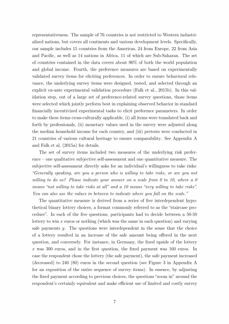
In sum, conditioning on a large set of economic, institutional, geographic, climatic,and demographic variables, the relationship between genetic distance and differencesin risk preferences is highly significant. Furthermore, the corresponding point esti-mate is rather robust: While the coefficient is 0.26 in the full regression model, it is0.37 in the unconditional regression. Following the work of Altonji et al. (2005) andBellows and Miguel (2009), this observation can also be used to assess the extent towhich unobservable omitted variables likely bias our result. These authors show thatby comparing the coefficients in the unconditional and the full regression model, theratio β̂full

β̂unconditional−β̂fullyields an estimate of how much larger the bias arising from

unobservable factors would need to be relative to the bias resulting from observables,in oder to generate the observed coefficient if the true coefficient was actually zero. Ifthis ratio equals α, then omitted variables can only explain the observed coefficientif the bias resulting from unobservables equals at least α times the bias resultingfrom observed variables. In our case, comparing the coefficients in columns (1) and(6) of Table 3, the ratio equals 2.4.21 Thus, if the genetic distance coefficient wasto be explained away by selection on unobservables, then this bias would have to beat least 2.4 times as strong as selection on the very large and comprehensive set ofcovariates that we included in our regressions.

4.4 Robustness

While the majority of the genetic distances in our sample are relatively small, we alsoobserve a number of large genetic distances. To ensure that our results are not drivenby these large distances, we pursue two distinct strategies. First, using the samespecification as in our full regression model in column (6) of Table 3, we exclude thelargest genetic distances step-by-step. Second, we reduce the magnitude of differencesin genetic distances by estimating a log-log relationship between differences in riskpreferences and genetic distance. Columns (1) through (4) of Table 4 present theresults of the regressions utilizing the restricted samples, which demonstrate thatexcluding large distances does not affect the statistical significance of our result.Furthermore, column (13) shows that the spirit of our results is unaffected in alog-log specification.

Our control variables already accounted for the presence of differences in continentfixed effects. To provide further evidence that no single region drives our result,columns (5) through (12) of Table 4 present the results from regressions which exclude

21The ratio is the same if we consider the common sample from the specifications fromcolumns (1) and (6) in Table 3.

20

the four major regions of the world one-by-one. In most specifications, the resultsremain statistically significant despite the large drop in the number of observations,and conditional on the full set of covariates.

In Appendix C.1 we provide further robustness checks by employing differentdependent variables than the absolute difference in average risk attitudes. First, weshow that our main result continues to hold when we use the absolute difference inthe 25th, 50th or 75th percentile of risk aversion as dependent variable. Second,recall that our index of risk aversion consists of a linear combination of two types ofsurvey items, a qualitative self-assessment and a series of quantitative binary lotterychoices. By employing both items separately, we show that the effect of temporaldistance on risk preferences is not specific to a particular type of survey question.

4.5 Alternative Measures

Up to this point, all of our multivariate regressions were conducted using the rawFST genetic distance. We now present a set of regressions which utilize additionalinformation on the measurement precision of the genetic distance data. Since thedata on allele frequencies are collected from different sample sizes across countries,the precision of the measurement varies across country pairs. Thus, using bootstrapanalysis, Cavalli-Sforza et al. (1994) compute standard errors of the FST genetic dis-tance for each pair. Following the methodology proposed by Spolaore and Wacziarg(2009), we utilize this information by linearly downweighing each observation by itsstandard error (see Appendix D). The results from the corresponding weighted leastsquares regression, are presented in columns (1)-(3) of Table 10. The resulting stan-dardized beta coefficients are highly significant and very similar to those from theunweighted regressions, providing reassuring evidence that our results are not drivenby measurement error.

Section 4.1 showed that the raw relationship between temporal distance anddifferences in risk preferences also holds when employing the Nei genetic distanceor migratory distance measures as proxies. Columns (4)-(12) establish that theseraw correlations are robust to the full set of covariates. Notably, the results obtainedwith the predicted measures of migratory distance further emphasize that it is indeedancient migration patterns rather than genetic distance as such which is at the coreof our analysis.22

22In contrast, when we employ linguistic distance in the conditional regressions, we obtain smalland insignificant coefficients. This is consistent with the idea that the coarse and noisy constructionof linguistic distances introduces severe measurement error and is hence an inferior proxy for timingof separation as compared to genetic or predicted migratory distance data.

21

Tab

le4:

Rob

ustness:

Exclude

largegeneticdistan

cesor

continents

Dependent

variable:

Absolutediffe

rencein

averag

erisk

aversion

Restrictedsample:

Fst<

Exclude

continents

Log[A

bs.diffe

rence

Baseline

<0.85

<0.7

<0.5

Americas

EU

&Central

Asia

SEAsia&

Pacific

Africa&

ME

inrisk

attitudes]

(1)

(2)

(3)

(4)

(5)

(6)

(7)

(8)

(9)

(10)

(11)

(12)

(13)

Fstgeneticdistan

ce0.26

∗∗∗

0.31

∗∗∗

0.41

∗∗∗

0.40

∗∗∗

0.36

∗∗∗

0.25

∗∗0.22

∗∗0.13

0.36

∗∗∗

0.34

∗∗∗

0.15

0.25

∗∗

(0.10)

(0.10)

(0.11)

(0.11)

(0.10)

(0.10)

(0.09)

(0.10)

(0.09)

(0.12)

(0.10)

(0.11)

Log[Fst

geneticdistan

ce]

0.17

∗∗

(0.07)

Con

stan

t-0.34

-0.28

-0.22

-0.37

0.21

-0.90

0.43

0.39

0.06

7-0.85

0.26

0.26

-2.91

(0.63)

(0.64)

(0.64)

(0.70)

(0.66)

(0.69)

(0.76)

(0.73)

(0.77)

(0.76)

(0.49)

(0.59)

(1.90)

Dem

ograph

ican

decon

omic

controls

Yes

Yes

Yes

Yes

Yes

Yes

Yes

Yes

Yes

Yes

Yes

Yes

Yes

Geograp

hic,

clim

atean

dhealth

controls

Yes

Yes

Yes

Yes

No

Yes

No

Yes

No

Yes

No

Yes

Yes

Con

tinent

FE

Yes

Yes

Yes

Yes

No

No

No

No

No

No

No

No

Yes

Observation

s25

5624

8322

5819

2516

5316

5310

8110

8117

1117

1113

2613

2625

56R

20.32

90.32

90.29

70.20

90.17

10.28

70.11

00.20

70.18

30.28

50.03

10.07

90.23

5Stan

dardized

beta

(%)

23.2

25.8

29.4

24.4

32.4

22.4

20.1

12.2

31.5

29.8

12.0

20.5

16.4

OLS

estimates,twow

ay-clustered

stan

dard

errors

inpa

rentheses.

EU

=Europ

e,ME=

MiddleEast,SE

Asia=

SouthAsiaan

dSo

uth-EastAsia.

The

variab

lesin

logs

aredefin

edasln

[0.0

1+x

],wherexdeno

testheoriginal

variab

le.SeeTa

bles

2an

d3foracompletelistof

thedemog

raph

ic,e

cono

mic,g

eograp

hic,

clim

atic,a

ndhealth

controlv

ariables.The

stan

dardized

betasreferto

geneticdistan

ce.

∗p<

0.10

,∗∗p<

0.05

,∗∗∗p<

0.01

.

22

Tab

le5:

Alterna

tive

measuresan

destimationtechniqu

es

Dependent

variable:

Absolutediffe

rencein

averagerisk

aversion

WLS

OLS

WLS

OLS

OLS

(1)

(2)

(3)

(4)

(5)

(6)

(7)

(8)

(9)

(10)

(11)

(12)

Fstgeneticdistan

ce0.34

∗∗∗

0.25

∗∗∗

0.33

∗∗∗

(0.09)

(0.09)

(0.09)

Nei

geneticdistan

ce0.27

∗∗∗

0.26

∗∗∗

0.34

∗∗∗

0.26

∗∗∗

0.34

∗∗∗

(0.09)

(0.09)

(0.10)

(0.09)

(0.10)

Predicted

migratory

distan

ce0.87

∗∗∗

1.31

∗∗∗

(0.33)

(0.41)

HMImigratory

distan

ce0.69

∗∗∗

0.67

∗∗

(Özak,

2010)

(0.20)

(0.28)

Con

stan

t0.22

∗∗∗

-0.31

-0.31

-0.26

-0.31

0.23

∗∗∗

-0.21

-0.26

-0.26

-0.23

-0.031

-0.17

(0.03)

(0.71)

(0.66)

(0.69)

(0.64)

(0.03)

(0.71)

(0.68)

(0.68)

(0.62)

(0.84)

(0.77)

Dem

ograph

ican

decon

omic

controls

No

Yes

Yes

Yes

Yes

No

Yes

Yes

Yes

Yes

Yes

Yes

Geograp

hic,

clim

atean

dhealth

controls

No

Yes

Yes

Yes

Yes

No

Yes

Yes

Yes

Yes

Yes

Yes

Con

tinent

FE

No

No

Yes

No

Yes

No

No

Yes

No

Yes

No

Yes

Observation

s2628

2556

2556

2556

2556

2628

2556

2556

2556

2556

2016

2016

R2

0.074

0.186

0.283

0.244

0.327

0.059

0.162

0.256

0.236

0.328

0.268

0.355

Stan

dardized

beta

(%)

27.3

20.5

26.9

23.2

22.0

24.3

18.5

23.6

14.1

21.3

25.0

24.5

OLS

estimates,tw

oway-clustered

stan

dard

errors

inpa

rentheses.

The

weigh

ted

least-squa

resregression

slin

earlydo

wnw

eigh

observations

bythe

stan

dard

errorof

therespective

geneticdistan

ceestimate,

asob

tained

from

bootstrapan

alysis

byCavalli-Sforza

etal.(1994),seeApp

endixD

for

details.SeeTa

bles

2an

d3foracompletelistof

thedemograph

ic,econ

omic,geograph

ic,clim

atic,an

dhealth

controlvariab

les.

The

stan

dardized

betasreferto

thetempo

rald

istanceprox

ies.

∗p<

0.10

,∗∗p<

0.05

,∗∗∗p<

0.01

.

23

5 Preference Heterogeneity and Migratory Distance

from East Africa

The final step of our analysis considers the relationship between the within-populationvariability in risk preferences and migratory distance from Africa. To this end, weestimate the following equation:

σi = α + β × Predicted migratory distance from Ethiopiai + γ × xi + εi

where σi denotes the standard deviation in risk attitudes within a country, xia vector of covariates, and εi a disturbance term. Table 6 provides an overview ofthe results of corresponding OLS regressions. In columns (1)-(4), we use predictedmigratory distance from Ethiopia (constructed as described in Section 3.2) as ex-planatory variable, while columns (5) through (8) employ the migratory distancemeasure which is based on the human mobility index.

Column (1) indicates that the average total length of the migration path of agiven population from East Africa exhibits a raw correlation with the standard devi-ation in risk attitudes. Columns (2) through (3) add several control variables to thebaseline specification, which capture cross-country differences in sociodemographics,development, geography, and climate. The details of the corresponding regressions,i.e., the coefficients of the covariates, can be found in Appendix E. The results showthat, if anything, conditioning on this vector of covariates strengthens the correlationbetween preference heterogeneity and migratory distance. However, as column (4)indicates, the inclusion of continental fixed effects leads the coefficient of migratorydistance to drop in size and to become insignificant. By the serial founder effect andthe paths of human migration, continent dummies are correlated with migratory dis-tance from East Africa and take out a substantial fraction of the variation not onlyin migratory distance but also in preference heterogeneity. Columns (5) through (8)repeat the same specifications using the more sophisticated mobility index-adjustedmeasure of migratory distance. Consistent with measurement error in the baselinemigratory distance measure biasing the coefficient towards zero, the results are, ifanything, even stronger, and remain weakly significant even under continent fixedeffects. Figure 5 in Appendix E provides a graphical illustration of the correspondingraw relationship.

Taken together, our second set of results shows that ancient migration patternsare not only reflected in cross-country differences in average risk aversion, but alsoin the dispersion of the preference pool.

24

Table 6: Preference dispersion and migratory distance from East Africa

Dependent variable: SD in risk aversion(1) (2) (3) (4) (5) (6) (7) (8)

Migratory distance from Ethiopia -0.52∗ -0.83∗∗ -0.64∗ -0.15(0.28) (0.32) (0.36) (0.47)

HMI migratory distance from Ethiopia -0.52∗∗ -0.77∗∗∗ -0.73∗∗ -0.80∗

(Özak, 2010) (0.21) (0.26) (0.29) (0.45)

Constant 0.98∗∗∗ 0.11 1.16∗∗ 0.80 1.00∗∗∗ -0.47 1.36∗∗ 1.51∗∗(0.02) (0.42) (0.52) (0.62) (0.02) (0.56) (0.62) (0.70)

Socioeconomic controls No Yes Yes Yes No Yes Yes Yes

Geographic controls No No Yes Yes No No Yes Yes

Continent FE No No No Yes No No No Yes

Observations 73 73 73 73 64 64 64 64R2 0.048 0.380 0.509 0.568 0.074 0.412 0.578 0.595Standardized beta (%) -21.8 -34.6 -26.9 -6.4 -27.2 -40.0 -37.9 -41.5

OLS estimates, robust standard errors in parentheses. In columns (2) and (6), the additional controls includeaverage age, proportion of females, log (GDP p/c) and its square, SD in age, a gender heterogeneity index, SDin (log) household income, (log) population size, linguistic diversity and life expectancy. Columns (3) and (7)additionally include distance to the equator, temperature, precipitation, suitability for agriculture, the fractionof the population at risk of contracting malaria, and the log of the timing of the Neolithic revolution, whilecolumns (4) and (8) add continent fixed effects. ∗ p < 0.10, ∗∗ p < 0.05, ∗∗∗ p < 0.01.

6 Conclusion

We analyze the distribution of risk preferences of representative population samplesin countries spanning all continents. The main contribution of this paper is toestablish that, along two dimensions, a significant fraction of the substantial between-country heterogeneity has its deep historical origins in ancestral migration patterns.As for average risk attitudes, we show that three classes of proxies for the length oftime since two populations shared common ancestors are predictive of how similartwo countries’ risk preferences are. Regarding within-country heterogeneity, we showthat the migratory distance from East Africa predicts the dispersion of the preferencedistribution.

A growing body of empirical work highlights the importance of heterogeneity inrisk preferences for understanding a myriad of economic and health behaviors atthe individual level. However, it remains an open question whether country-levelrisk preferences are related to the cross-country variation in economic, institutional,and health-related outcomes. In our data, average risk aversion is indeed predictiveof variables that one would intuitively expect to be associated with risk attitudes.Specifically, more risk-tolerant societies tend to live in more risky economic, institu-tional, and health environments (see Falk et al., 2015a, and Appendix F). Regardingeconomic risks, high risk taking is associated with high income inequality (Gini index,income share of the top 10%) and a high risk of living in poverty, i.e., on less than

25

$2 per day, conditional on per capita income. Similarly, risk averse populations tendto live in institutional structures which provide strong labor protection against, e.g.,unemployment. Similarly, as for health risks, a higher risk tolerance is significantlyrelated to a higher prevalence of HIV, traffic death rates, and lower life expectancy.The latter relationship is depicted in the left-hand panel of Figure 2. Thus, in sum,risk averse socities appear to live in environments which are intuitively less risky, pro-viding suggestive evidence that the cross-country heterogeneity in risk preferencesmight have important consequences not just for individual decision making.

However, it is conceivable that not just the level of risk aversion in a given coun-try has economic effects, but also the corresponding variability. Indeed, Ashraf andGalor (2013b) argue for the importance of cultural diversity in explaining compara-tive development around the globe. Recall that these authors show that per capitaincome is hump-shaped in the diversity of the respective genetic pool (which is atransformation of migratory distance from East Africa). Given our finding that thewithin-country dispersion in the pool of risk preferences decreases in migratory dis-tance from East Africa, and hence increases in the diversity of the genetic pool, it isa natural question to ask whether there is a relationship between the variability inrisk attitudes and economic development. The right-hand panel of Figure 2 showsthat per capita income monotonically decreases in the standard deviation of riskattitudes, with a raw correlation of ρ = −0.32, p < 0.01. As we show in Appendix F,this correlation is very robust and holds up when we condition on continent fxiedeffects, a large number of geographic and climatic covariates, genetic diversity andits square, ethnic or linguistic fractionalization or even institutional quality and av-erage years of schooling. In fact, as we show in the Appendix, this correlation ismuch stronger when we consider the standard deviation in the quantitative choice

AFG

AREARG

AUSAUT

BGD

BIH

BOL

BRA

BWA

CANCHECHL

CHN

CMR

COL

CRICZE

DEU

DZAEGY

ESP

EST

FINFRA

GBR

GEO

GHA

GRC

GTM

HRV

HTI

HUN

IDN

IND

IRNIRQ

ISRITA

JOR

JPN

KAZ

KEN

KHM

KOR

LKALTU

MARMDA

MEX

MWINGA

NIC

NLD

PAK

PER

PHL

POLPRT

ROU

RUS

RWA

SAUSRB

SUR

SWE

THA TUR

TZAUGA

UKR

USA

VENVNM

ZAF

ZWE

4050

6070

80Li

fe e

xpec

tanc

y at

birt

h

-1 -.5 0 .5 1Willingness to take risks

Risk taking and life expectancy

AFG

ARE

ARG

AUS AUT

BGD

BIH

BOL

BRABWA

CANCHE

CHL

CHN

CMR

COLCRI

CZE

DEU

DZA

EGY

ESP

EST

FINFRA GBR

GEO

GHA

GRC

GTM

HRV

HTI

HUN

IDNIND

IRNIRQ

ISRITA

JOR

JPN

KAZ

KENKHM

KOR

LKA

LTU

MAR

MDA

MEX

MWI

NGANIC

NLD

PAK

PER

PHL

POL

PRT

ROU RUS

RWA

SAU

SRBSUR

SWE

THA

TUR

TZAUGA

UKR

USA

VEN

VNM

ZAF

ZWE

46

810

12Lo

g [G

DP p

/c P

PP]

.7 .8 .9 1 1.1 1.2SD in willingness to take risks

SD in risk taking and per capita income

Figure 2: Risk attitudes, health and economic outcomes. The left panel depicts the raw correlationbetween life expectancy at birth and risk taking, while the right panel depicts the relationshipbetween (log) per capita income and the standard deviation in risk aversion.

26

procedure only.In sum, both the first and second moment of the within-country distribution

of risk preferences are associated with heterogeneous economic, institutional, andhealth outcomes. Our results highlight that if we aim to understand the ultimateroots of the underlying preference heteroegeneity, we might have to consider eventsvery far back in time.

27

References

Alesina, Alberto, Arnaud Devleeschauwer, William Easterly, SergioKurlat, and Romain Wacziarg, “Fractionalization,” Journal of EconomicGrowth, 2003, 8 (2), 155–194.

, Paola Giuliano, and Nathan Nunn, “On the Origins of Gender Roles: Womenand the Plough,” Quarterly Journal of Economics, 2013, 128 (2), 469–530.

Altonji, Joseph G., Todd E. Elder, and Christopher R. Taber, “Selectionon Observed and Unobserved Variables: Assessing the Effectiveness of CatholicSchools,” Journal of Political Economy, 2005, 113 (1), 151–184.

Arbatli, Cemal Eren, Quamrul Ashraf, and Oded Galor, “The Nature ofCivil Conflict,” Working Paper, 2013.

Ashraf, Quamrul and Oded Galor, “Genetic Diversity and the Origins of CulturalFragmentation,” American Economic Review: Papers & Proceedings, 2013, 103 (3),528–33.

and , “The Out of Africa Hypothesis, Human Genetic Diversity, and Compar-ative Economic Development,” American Economic Review, 2013, 103 (1), 1–46.

, , and Marc P. Klemp, “The Out of Africa Hypothesis of ComparativeDevelopment Reflected by Nighttime Light Intensity,” Working Paper, 2014.

Barro, Robert J. and Jong-Wha Lee, “A New Data Set of Educational Attain-ment in the World, 1950–2010,” Journal of Development Economics, 2012.

Bellows, John and Edward Miguel, “War and Local Collective Action in SierraLeone,” Journal of Public Economics, 2009, 93 (11), 1144–1157.

Botero, Juan, Simeon Djankov, Rafael LaPorta, Florencio Lopezde Silanes, and Andrei Shleifer, “The Regulation of Labor,” Quarterly Journalof Economics, 2004, 119 (4), 1339–1382.

Callen, Michael, Mohammad Isaqzadeh, James D. Long, and CharlesSprenger, “Violence and Risk Preference: Experimental Evidence fromAfghanistan,” American Economic Review, 2014, 104 (1), 123–148.

Cameron, A. Colin, Jonah B. Gelbach, and Douglas L. Miller, “RobustInference with Multiway Clustering,” Journal of Business & Economic Statistics,2011, 29 (2).

28

Cavalli-Sforza, Luigi L., “Genes, Peoples, and Languages,” Proceedings of theNational Academy of Sciences, 1997, 94 (15), 7719–7724.

Cavalli-Sforza, Luigi, Paolo Menozzi, and Alberto Piazza, The History andGeography of Human Genes, Princeton university press, 1994.

Cesarini, David, Christopher T. Dawes, Magnus Johannesson, Paul Licht-enstein, and Björn Wallace, “Genetic Variation in Preferences for Giving andRisk Taking,” Quarterly Journal of Economics, 2009, 124 (2), 809–842.

Chen, M. Keith, “The Effect of Language on Economic Behavior: Evidence fromSavings Rates, Health Behaviors, and Retirement Assets,” American EconomicReview, 2013, 103 (2), 690–731.

Desmet, Klaus, Ignacio Ortuno-Ortin, and Romain Wacziarg, “Culture,Ethnicity and Diversity,” Working Paper, 2014.

, Michel Le Breton, Ignacio Ortuno-Ortin, and Shlomo Weber, “TheStability and Breakup of Nations: A Quantitative Analysis,” Journal of EconomicGrowth, 2011, 16, 183–213.

Dohmen, Thomas, Armin Falk, David Huffman, and Uwe Sunde, “TheIntergenerational Transmission of Risk and Trust Attitudes,” Review of EconomicStudies, 2012, 79 (2), 645–677.

, , , , Jürgen Schupp, and Gert G. Wagner, “Individual Risk At-titudes: Measurement, Determinants, and Behavioral Consequences,” Journal ofthe European Economic Association, 2011, 9 (3), 522–550.

Falk, Armin, Anke Becker, Thomas Dohmen, Benjamin Enke, Uwe Sunde,and David Huffman, “The Nature of Human Preferences: Global Evidence,”Working Paper, 2015.

, , , David Huffman, and Uwe Sunde, “An Experimentally ValidatedSurvey Module of Economic Preferences,” Working Paper, 2015.

Fearon, James, “Is Genetic Distance a Plausible Measure of Cultural Distance?,”unpublished, Stanford University, 2006.

Fearon, James D., “Ethnic and Cultural Diversity by Country,” Journal of Eco-nomic Growth, 2003, 8 (2), 195–222.

29

Fehr, Ernst and Karla Hoff, “Introduction: Tastes, Castes and Culture: theInfluence of Society on Preferences,” Economic Journal, 2011, 121 (556), F396–F412.

Fernández, Raquel and Alessandra Fogli, “Fertility: The Role of Culture andFamily Experience,” Journal of the European Economic Association, 2006, 4 (2-3),552–561.

and , “Culture: An Empirical Investigation of Beliefs, Work, and Fertility,”American Economic Journal: Macroeconomics, 2009, 1 (1), 146–177.

Gallup, John L., Jeffrey D. Sachs, and Andrew D. Mellinger, “Geographyand Economic Development,” International Regional Science Review, 1999, 22 (2),179–232.

, et al., “The Economic Burden of Malaria.,” American Journal of TropicalMedicine and Hygiene, 2000, 64 (1-2 Suppl), 85–96.

Galor, Oded and Ömer Özak, “The Agricultural Origins of Time Preference,”Working Paper, 2014.

Giuliano, Paola, Antonio Spilimbergo, and Giovanni Tonon, “Genetic Dis-tance, Transportation Costs, and Trade,” Journal of Economic Geography, 2014,14 (1), 179–198.

Gorodnichenko, Yuriy and Gerard Roland, “Culture, Institutions and theWealth of Nations,” Working Paper, 2010.

Guiso, Luigi, Paola Sapienza, and Luigi Zingales, “Does Culture Affect Eco-nomic Outcomes?,” Journal of Economic Perspectives, 2006, 20 (2), 23–48.

, , and , “Cultural Biases in Economic Exchange?,” Quarterly Journal ofEconomics, 2009, 124 (3), 1095–1131.

Henn, Brenna M., Luigi L. Cavalli-Sforza, and Marcus W. Feldman, “TheGreat Human Expansion,” Proceedings of the National Academy of Sciences, 2012,109 (44), 17758–17764.

Mecham, R. Quinn, James Fearon, and David Laitin, “Religious Classificationand Data on Shares of Major World Religions,” unpublished, Stanford University,2006, 1 (5), 18.

Michalopoulosa, Stelios, “The Origins of Ethnolinguistic Diversity,” AmericanEconomic Review, 2012, 102 (4), 1508–1539.

30

Nordhaus, William D., “Geography and Macroeconomics: New data and newFindings,” Proceedings of the National Academy of Sciences of the United Statesof America, 2006, 103 (10), 3510–3517.

Nunn, Nathan and Leonard Wantchekon, “The Slave Trade and the Origins ofMistrust in Africa,” American Economic Review, 2011, 101 (7), 3221–52.

Özak, Ömer, “The Voyage of Homo-Oeconomicus: Some Economic Measures ofDistance,” Working Paper, 2010.

Proto, Eugenio and Andrew J. Oswald, “National Happiness and Genetic Dis-tance: A Cautious Exploration,” Working Paper, 2014.

Putterman, Louis and David N. Weil, “Post-1500 Population Flows and theLong-Run Determinants of Economic Growth and Inequality,” Quarterly Journalof Economics, 2010, 125 (4), 1627–1682.

Ramachandran, Sohini, Omkar Deshpande, Charles C. Roseman, Noah A.Rosenberg, Marcus W. Feldman, and L. Luca Cavalli-Sforza, “Supportfrom the Relationship of Genetic and Geographic Distance in Human Populationsfor a Serial Founder Effect Originating in Africa,” Proceedings of the NationalAcademy of Sciences of the United States of America, 2005, 102 (44), 15942–15947.

Rieger, Marc Oliver, Mei Wang, and Thorsten Hens, “Risk PreferencesAround the World,” Management Science, 2014.

Spolaore, Enrico and Romain Wacziarg, “The Diffusion of Development,” Quar-terly Journal of Economics, 2009, 124 (2), 469–529.

and , “Long-Term Barriers to the International Diffusion of Innovations,” in“NBER International Seminar on Macroeconomics 2011” University of ChicagoPress 2011, pp. 11–46.

and , “War and Relatedness,” Working Paper, 2014.

Tabellini, Guido, “Institutions and Culture,” Journal of the European EconomicAssociation, 2008, 6 (2-3), 255–294.

Vieider, Ferdinand M., Mathieu Lefebvre, Ranoua Bouchouicha, ThorstenChmura, Rustamdjan Hakimov, Michal Krawczyk, and Peter Martins-son, “Common Components of Risk and Uncertainty Attitudes Across Contextsand Domains: Evidence from 30 Countries,” Journal of the European EconomicAssociation, forthcoming.

31

, Thorsten Chmura, and Peter Martinsson, “Risk Attitudes, Development,and Growth: Macroeconomic Evidence from Experiments in 30 Countries,” Dis-cussion Paper, Social Science Research Center Berlin, 2012.

Voigtländer, Nico and Hans-Joachim Voth, “Persecution Perpetuated: TheMedieval Origins of Anti-Semitic Violence in Nazi Germany,” Quarterly Journalof Economics, 2012, 127 (3), 1339–1392.

32

ONLINE APPENDIX

A Details on Data Collection of Risk Preferences

The description of the dataset builds on Falk et al. (2015a).

A.1 Overview

The cross-country dataset covering risk aversion, patience, positive and negativereciprocity, altruism, and trust, was collected through the professional infrastructureof the Gallup World Poll 2012. The data collection process essentially consistedof three steps. First, we conducted a laboratory experimental validation procedureto select the survey items. Second, Gallup implemented a pre-test in a variety ofcountries to ensure the implementability of our items in a culturally diverse sample.Third, the data were collected through the regular professional data collection effortsin the framework of the World Poll 2012.

A.2 Experimental Validation

To ensure the behavioral relevance of our preference measures, all underlying sur-vey items were selected through an experimental validation procedure. To this end,a sample of German undergraduates completed standard state-of-the-art financiallyincentivized laboratory experiments designed to measure risk aversion, patience, pos-itive and negative reciprocity, altruism, and trust. The same sample of subjects thencompleted a large battery of potential survey items. In a final step, for each pref-erence, those survey items were selected which jointly perform best in predictingfinancially incentivized behavior. See Falk et al. (2015a) for details. The resultingset of items was then adjusted in the process of a pre-test.

A.3 Pre-Test

Prior to including the preference module in the Gallup World Poll 2012, it wastested in the field as part of the World Poll 2012 pre-test, which was conductedat the end of 2011 in 22 countries. The main goal of the pre-test was to receivefeedback and comments on each item from various cultural backgrounds in orderto assess potential difficulties in understanding and differences in the respondents’interpretation of items. Based on respondents’ feedback and suggestions, severalitems were modified in terms of wording before running the survey as part of theWorld Poll 2012.

33

The pre-test was run in 10 countries in central Asia (Russia, Belarus, Kyrgyzs-tan, Azerbaijan, Georgia, Tajikistan, Uzbekistan, Kazakhstan, Armenia, and Turk-menistan), 2 countries in South-East Asia (Bangladesh and Cambodia), 5 countriesin Southern and Eastern Europe (Croatia, Hungary, Poland, Romania, Turkey), 4countries in the Middle East and North Africa (Saudi-Arabia, Lebanon, Jordan, Al-geria), and 1 country in Eastern Africa (Kenya). In each country, the sample sizewas 10 to 15 people. Overall, more than 220 interviews were conducted. In mostcountries, the sample was mixed in terms of gender, age, educational background,and area of residence (urban / rural).

Participants of the pre-test were asked to state any difficulties in understandingthe items and to rephrase the meaning of items in their own words. If encounteringdifficulties in understanding or interpretations of items that were not intended, re-spondents were asked to make suggestions on how to modify the wording of the itemin order to attain the desired meaning.

Overall, the understanding of both the qualitative items and the quantitativeitems was good. In particular, no interviewer received any complaints regardingdifficulties in assessing the quantitative questions. When asked for rephrasing thequalitative item in their own words, most participants seemed to have understoodthe item in exactly the way that was intended.

However, when being confronted with hypothetical choices between monetaryamounts today versus larger amounts one year later, some participants, especiallyin countries with current or relatively recent phases of volatile and high inflationrates, stated that their answer would depend on the rate of inflation, or said thatthey would always take the immediate payment due to uncertainty with respectto future inflation. Therefore, we decided to adjust the wording, relative to the“original” experimentally validated item, by adding the phrase “Please assume thereis no inflation. i.e. future prices are the same as today’s prices” to each questioninvolving hypothetical choices between immediate and future monetary amounts.

A.4 Selection of Countries

Our goal when selecting countries was to ensure representativeness for the global pop-ulation. Thus, we chose countries from each continent and each region within con-tinents. In addition, we aimed at maximizing variation with respect to observables,such as GDP per capita, language, historical and political characteristics, or geo-graphical location and climatic conditions. Accordingly, we favored non-neighboringand culturally dissimilar countries. This procedure resulted in the following sampleof 76 countries:

34

East Asia and Pacific: Australia, Cambodia, China, Indonesia, Japan, Philippines,South Korea, Thailand, VietnamEurope and Central Asia: Austria, Bosnia and Herzegovina, Croatia, Czech Re-public, Estonia, Finland, France, Georgia, Germany, Greece, Hungary, Italy, Kaza-khstan, Lithuania, Moldova, Netherlands, Poland, Portugal, Romania, Russia, Ser-bia, Spain, Sweden, Switzerland, Turkey, Ukraine, United KingdomLatin America and Caribbean: Argentina, Bolivia, Brazil, Chile, Colombia, CostaRica, Guatemala, Haiti, Mexico, Nicaragua, Peru, Suriname, VenezuelaMiddle East and North Africa: Algeria, Egypt, Iran, Iraq, Israel, Jordan, Morocco,Saudi Arabia, United Arab EmiratesNorth America: United States, CanadaSouth Asia: Afghanistan, Bangladesh, India, Pakistan, Sri LankaSub-Saharan Africa: Botswana, Cameroon, Ghana, Kenya, Malawi, Nigeria, Rwanda,South Africa, Tanzania, Uganda, Zimbabwe

A.5 Sampling and Survey Implementation

A.5.1 Background

Since 2005, the international polling company Gallup conducts an annual WorldPoll, in which it surveys representative population samples in almost every countryaround the world on, e.g., economic, social, political, and environmental issues. Thecollection of our preference data was embedded into the regular World Poll 2012and hence made use of the pre-existing polling infrastructure of one of the largestprofessional polling institutes in the world.23

A.5.2 Survey Mode

Interviews were conducted via telephone and face-to-face. Gallup uses telephone sur-veys in countries where telephone coverage represents at least 80% of the populationor is the customary survey methodology. In countries where telephone interviewingis employed, Gallup uses a random-digit-dial method or a nationally representativelist of phone numbers. In countries where face-to-face interviews are conducted,households are randomly selected in an area-frame-design.

23Comparehttp://www.gallup.com/strategicconsulting/156923/worldwide-research-methodology.aspx

35

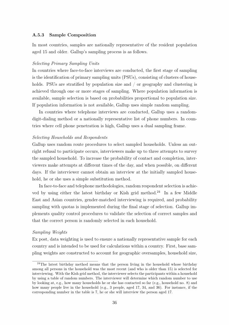
A.5.3 Sample Composition

In most countries, samples are nationally representative of the resident populationaged 15 and older. Gallup’s sampling process is as follows.

Selecting Primary Sampling UnitsIn countries where face-to-face interviews are conducted, the first stage of samplingis the identification of primary sampling units (PSUs), consisting of clusters of house-holds. PSUs are stratified by population size and / or geography and clustering isachieved through one or more stages of sampling. Where population information isavailable, sample selection is based on probabilities proportional to population size.If population information is not available, Gallup uses simple random sampling.

In countries where telephone interviews are conducted, Gallup uses a random-digit-dialing method or a nationally representative list of phone numbers. In coun-tries where cell phone penetration is high, Gallup uses a dual sampling frame.

Selecting Households and RespondentsGallup uses random route procedures to select sampled households. Unless an out-right refusal to participate occurs, interviewers make up to three attempts to surveythe sampled household. To increase the probability of contact and completion, inter-viewers make attempts at different times of the day, and when possible, on differentdays. If the interviewer cannot obtain an interview at the initially sampled house-hold, he or she uses a simple substitution method.

In face-to-face and telephone methodologies, random respondent selection is achie-ved by using either the latest birthday or Kish grid method.24 In a few MiddleEast and Asian countries, gender-matched interviewing is required, and probabilitysampling with quotas is implemented during the final stage of selection. Gallup im-plements quality control procedures to validate the selection of correct samples andthat the correct person is randomly selected in each household.

Sampling WeightsEx post, data weighting is used to ensure a nationally representative sample for eachcountry and is intended to be used for calculations within a country. First, base sam-pling weights are constructed to account for geographic oversamples, household size,

24The latest birthday method means that the person living in the household whose birthdayamong all persons in the household was the most recent (and who is older than 15) is selected forinterviewing. With the Kish grid method, the interviewer selects the participants within a householdby using a table of random numbers. The interviewer will determine which random number to useby looking at, e.g., how many households he or she has contacted so far (e.g., household no. 8) andhow many people live in the household (e.g., 3 people, aged 17, 34, and 36). For instance, if thecorresponding number in the table is 7, he or she will interview the person aged 17.

36

and other selection probabilities. Second, post-stratification weights are constructed.Population statistics are used to weight the data by gender, age, and, where reliabledata are available, education or socioeconomic status.

A.5.4 Translation of Items

The preference module items were translated into the major languages of each targetcountry. The translation process involved three steps. As a first step, a translatorsuggested an English, Spanish or French version of a German item, depending onthe region. A second translator, being proficient in both the target language andin English, French, or Spanish. then translated the item into the target language.Finally, a third translator would review the item in the target language and translateit back into the original language. If semantic differences between the original itemand the back-translated item occurred, the process was adjusted and repeated untilall translators agreed on a final version.

A.5.5 Adjustment of Monetary Amounts in Quantitative Items

All items involving monetary amounts were adjusted to each country in terms oftheir real value. In each country, all monetary amounts were calculated to representthe same share of the country’s median income in local currency as the share of theamount in Euro of the German median income since the validation study had beenconducted in Germany. Monetary amounts used in the validation study with theGerman sample were round numbers in order to facilitate easy calculations and toallow for easy comparisons. In order to proceed in a similar way in all countries, werounded all monetary amounts to the next “round” number. While this necessarilyresulted in some (if very minor) variation in the real stake size between countries, itminimized cross-country differences in the difficulty of understanding the quantitativeitems due to differences in assessing the involved monetary amounts.

A.5.6 Staircase procedure

The sequence of survey questions that form the basis for the quantitative risk aver-sion measure is given by the “tree” logic depicted in Figure 3. In Germany, eachrespondent faced five interdependent choices between taking part in a 50:50 lotteryof receiving 300 euros or nothing and varying safe amounts of money. The valuesin the tree denote the safe amounts of money. The rightmost level of the tree (5thdecision) contains 16 distinct monetary amounts, so that responses can be classifiedinto 32 categories which are ordered in the sense that the (visually) lowest path /

37

endpoint indicates the highest level of risk aversion. As in the experimental valida-tion procedure in Falk et al. (2015b), we assign values 1-32 to these endpoints, with32 denoting the highest level of risk aversion.

A.6 Computation of Preference Measures

A.6.1 Cleaning and Imputation of Missings

In order to make maximal use of the available information in our data, missing surveyitems were imputed based on the following procedure:

If one survey item was missing, then the missing item was predicted using theresponses to the other item. The procedure was as follows:

• Qualitative question missing: We regress all available survey responses to thequalitative question on responses to the staircase task, and then use thesecoefficients to predict the missing qualitative items using the available staircaseitems.

• Staircase item missing: The imputation procedure was similar, but made ad-ditional use of the informational content of the responses of participants whostarted but did not finish the sequence of the five questions. If the respon-dent did not even start the staircase procedure, then imputation was done bypredicting the staircase measure based on answers to the qualitative surveymeasure using the methodology described above. On the other hand, if therespondent answered at least one of the staircase questions, the final staircaseoutcome was based on the predicted path through the staircase procedure. Sup-pose the respondent answered four items such that his final staircase outcomewould have to be either x or y. We then predict the expected choice between xand y based on a probit of the “x vs. y” decision on the qualitative item. If therespondent answered three (or less) questions, the same procedure was applied,the only difference being that in this case the obtained predicted probabilitieswere applied to the expected values of the staircase outcome conditional onreaching the respective node. Put differently, the procedure outlined abovewas applied recursively by working backwards through the “tree” logic of thestaircase procedure.

38

160

80

40

20

10Risk taking=1B

Risk taking=2AB

30Risk taking=3B

Risk taking=4A

AB

60

50Risk taking=5B

Risk taking=6AB

70Risk taking=7B

Risk taking=8A

A

A

B

120

100

90Risk taking=9B

Risk taking=10AB

110Risk taking=11B

Risk taking=12A

AB

140

130Risk taking=13B

Risk taking=14AB

150Risk taking=15B

Risk taking=16A

A

A

A

B

240

200

180

170Risk taking=17B

Risk taking=18AB

190Risk taking=19B

Risk taking=20A

AB

220

210Risk taking=21B

Risk taking=22AB

230Risk taking=23B

Risk taking=24A

A

A

B

280

260

250Risk taking=25B

Risk taking=26AB

270Risk taking=27B

Risk taking=28A

AB

300

290Risk taking=29B

Risk taking=30AB

310Risk taking=31B

Risk taking=32A

A

A

A

A

Figure 3: Tree for the staircase time task (numbers = payment in 12 months, A = choice of “100euros today”, B = choice of “x euros in 12 months”). The staircase procedure worked as follows.First, in Germany, each respondent was asked whether they would prefer to receive 160 eurosfor sure or whether they preferred a 50:50 chance of receiving 300 euros or nothing. In case therespondent opted for the safe choice (“B”), the safe amount of money being offered in the secondquestion decreased to 80 euros. If, on the other hand, the respondent opted for the gamble (“A”),the safe amount was increased to 240 euros. Working further through the tree follows the samelogic.

39

A.6.2 Computation of Preference Indices at Individual Level

We compute an individual-level index of patience by (i) computing the z-scores ofeach survey item at the individual level and (ii) weighing these z-scores using theweights resulting from the experimental validation procedure of Falk et al. (2015a).Technically, these weights are given by the coefficients of an OLS regression of ob-served behavior on responses to the respective survey items, such that the coefficientssum to one. These weights are given by (see above for the precise survey items):

Risk taking = 0.4729985× Staircase risk + 0.5270015× Qualitative item

A.6.3 Computation of Country Averages

In order to compute country-level averages, we weigh the individual-level data withthe sampling weights provided by Gallup, see above.

B Summary Statistics for Main Variables

Table 7: Summary statistics of main unilateral variables

Obs Mean SD Min Max

Average risk aversion 73 0.01 0.31 -0.79 0.97SD in risk aversion 73 0.94 0.09 0.75 1.18Predicted migratory distance from Ethiopia 73 0.07 0.04 0.01 0.19

Table 8: Summary statistics of main bilateral variables

Obs Mean SD Min Max

Abs. difference in avg. risk aversion 2628 0.34 0.27 0 1.76Fst genetic distance 2628 0.34 0.24 0 1Nei genetic distance 2628 0.30 0.23 0 1Predicted migratory distance 2628 0.08 0.04 0 0.23HMI migratory distance 2080 0.17 0.10 0.01 0.59Linguistic distance 2628 0.87 0.20 0 1

40

0.5

11.

5D

ensi

ty

-1 -.5 0 .5 1Average risk aversion

kernel = epanechnikov, bandwidth = 0.0908

Average risk aversion

0.5

11.

52

Den

sity

0 .5 1 1.5 2Abs. difference in average risk aversion

kernel = epanechnikov, bandwidth = 0.0488

Abs. difference in average risk aversion

0.5

11.

5D

ensi

ty

-1 -.5 0 .5 1SD in risk aversion

kernel = epanechnikov, bandwidth = 0.0908

SD in risk aversion

0.5

11.

52

Den

sity

0 .2 .4 .6 .8 1Fst genetic distance

kernel = epanechnikov, bandwidth = 0.0454

Fst genetic distance

05

1015

20D

ensi

ty

0 .05 .1 .15 .2Predicted migratory distance from Ethiopia

kernel = epanechnikov, bandwidth = 0.0067

Predicted migratory distance from Ethiopia

Figure 4: Kernel density estimates of main variables

41

Table 9: Raw correlations among bilateral variables

∆ Risk Fst dist Nei dist Pred migr dist HMI dist Ling. dist∆ average risk attitudes 1Fst genetic distance 0.343 1Nei genetic distance 0.358 0.945 1Predicted migratory distance 0.111 0.517 0.509 1HMI migratory distance 0.249 0.623 0.634 0.922 1Linguistic distance 0.147 0.457 0.408 0.105 0.210 1

C Additional Bilateral Regressions

C.1 Alternative Dependent Variable Specifications

This Appendix provides additional robustness checks on our results pertaining toaverage risk aversion. Column (1) of Table 10 restates our full regression model,i.e., the results of column (5) in Table 3. Columns (2) through (4) employ thesame regression specification, yet use the absolute difference in the 25th, 50th, and75th percentile of risk aversion as dependent variable. Interestingly, the results showthat the relationship between genetic distance and risk attitudes is not specific tothe mean of the distribution of risk preferences, but extends to other parts of thedistribution.

Recall that our main measure of a country’s average risk aversion consists ofa weighted average of two survey questions, a hypothetical staircase lottery task,and a qualitative question. Columns (5) through (10) demonstrate that our resultextends to using each of these survey questions separately. Specifically, columns (5)and (6) employ the absolute difference in the average qualitative self-assessmentas dependent variable, while columns (7) through (8) use the average outcome ofthe five-step lottery choice procedure. Finally, columns (9) and (10) present tworegressions which utilize only the first choice in the sequential lottery procedure, i.e.,(in Germany) the choice between 160 euros for sure and a 50-50 bet of receiving 300euros or nothing. While this measure ignores a lot of information that is containedin subsequent choices, the corresponding results show that even according to thisvery rough measure of risk attitudes does genetic distance explain about 10 % of thevariation in preferences.

C.2 Additional Control Variables

Column (1) of Table 11 reproduces our full between-country regression including allcontrol variables (i.e., column (5) of Table 3). Columns (2)-(4) introduce additional

42

covariates into the analysis, but the overall picture remains virtually unchanged.Column (5) presents an additional, very conservative, specification which employscountry fixed effects rather than regional fixed effects. Specifically, we construct73 dummies each equal to one if a given country is part of a country pair and zerootherwise. While the resulting point estimate is somewhat lower than in the previousregressions, it is still significant and features a standardized beta of 18.2 %.

43

Tab

le10:Alterna

tive

depe

ndentvariab

les

Dependent

variable:Absolutediffe

rencein...

Average

Percentiles

Self-assessment

Lotterychoices

(baseline)

25th

50th

75th

(average)

(average

outcom

e)(average

1stchoice)

(1)

(2)

(3)

(4)

(5)

(6)

(7)

(8)

(9)

(10)

Fstgeneticdistan

ce0.26

∗∗∗

0.33

∗∗∗

0.28

∗∗0.24

∗∗0.52

∗∗∗

0.53

∗∗3.02

∗∗∗

1.83

∗∗0.15

∗∗∗

0.091∗

∗

(0.10)

(0.12)

(0.11)

(0.10)

(0.14)

(0.21)

(1.03)

(0.89)

(0.05)

(0.04)

Con

stan

t-0.34

-0.64

-0.50

-0.26

0.74

∗∗∗

0.30

2.69

∗∗∗

-4.57

0.094∗

∗∗-0.30

(0.63)

(0.89)

(0.68)

(0.62)

(0.08)

(1.52)

(0.34)

(4.65)

(0.02)

(0.19)

Dem

ograph

ican

decon

omic

controls

Yes

Yes

Yes

Yes

No

Yes

No

Yes

No

Yes

Geograp

hic,

clim

atean

dhealth

controls

Yes

Yes

Yes

Yes

No

Yes

No

Yes

No

Yes

Con

tinent

FE

Yes

Yes

Yes

Yes

No

Yes

No

Yes

No

Yes

Observation

s2556

2556

2556

2556

2628

2556

2628

2556

2628

2556

R2

0.329

0.229

0.292

0.373

0.036

0.146

0.066

0.325

0.098

0.376

Stan

dardized

beta

(%)

23.2

25.8

22.5

18.4

18.9

19.3

25.6

15.9

31.3

19.1

OLS

estimates,tw

oway

-clustered

stan

dard

errors

inpa

rentheses.

The

depe

ndentvariab

lesconsistof

diffe

rent

measuresof

theab

solute

diffe

rencein

risk

attitudes:

(1)averages,(2)-(4)pe

rcentiles,

(5)-(6)average(qua

litative)

self-assessments,(7)-(8)averageou

tcom

eof

thestaircaselotterysequ

ence,(9)

-(10)averagedecision

infirst

lotterychoice

(safeam

ount

=160euros).Se

eTa

bles

2an

d3foracomplete

listof

thedemograph

ic,e

cono

mic,g

eograp

hic,

andclim

atic

controlv

ariables.The

stan

dardized

betasreferto

geneticdistan

ce.

∗p<

0.10

,∗∗p<

0.05

,∗∗∗p<

0.01

.

44

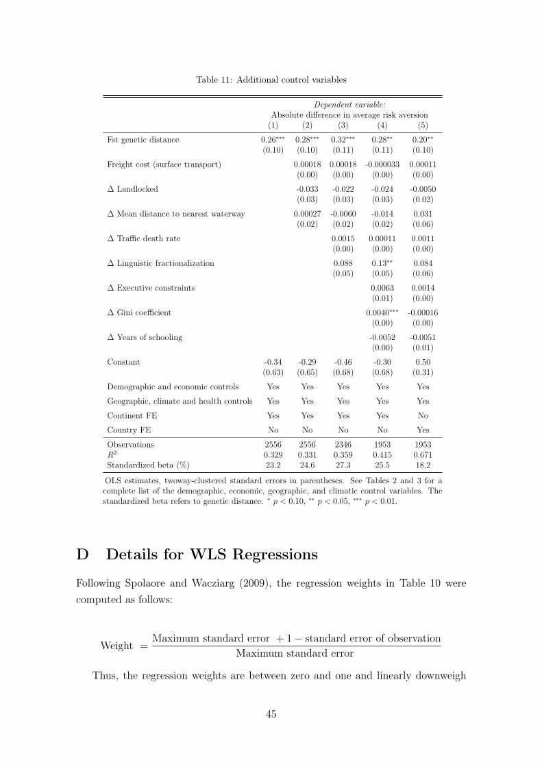
Table 11: Additional control variables

Dependent variable:Absolute difference in average risk aversion(1) (2) (3) (4) (5)

Fst genetic distance 0.26∗∗∗ 0.28∗∗∗ 0.32∗∗∗ 0.28∗∗ 0.20∗∗(0.10) (0.10) (0.11) (0.11) (0.10)

Freight cost (surface transport) 0.00018 0.00018 -0.000033 0.00011(0.00) (0.00) (0.00) (0.00)

∆ Landlocked -0.033 -0.022 -0.024 -0.0050(0.03) (0.03) (0.03) (0.02)

∆ Mean distance to nearest waterway 0.00027 -0.0060 -0.014 0.031(0.02) (0.02) (0.02) (0.06)

∆ Traffic death rate 0.0015 0.00011 0.0011(0.00) (0.00) (0.00)

∆ Linguistic fractionalization 0.088 0.13∗∗ 0.084(0.05) (0.05) (0.06)

∆ Executive constraints 0.0063 0.0014(0.01) (0.00)

∆ Gini coefficient 0.0040∗∗∗ -0.00016(0.00) (0.00)

∆ Years of schooling -0.0052 -0.0051(0.00) (0.01)

Constant -0.34 -0.29 -0.46 -0.30 0.50(0.63) (0.65) (0.68) (0.68) (0.31)

Demographic and economic controls Yes Yes Yes Yes Yes

Geographic, climate and health controls Yes Yes Yes Yes Yes

Continent FE Yes Yes Yes Yes No

Country FE No No No No Yes

Observations 2556 2556 2346 1953 1953R2 0.329 0.331 0.359 0.415 0.671Standardized beta (%) 23.2 24.6 27.3 25.5 18.2

OLS estimates, twoway-clustered standard errors in parentheses. See Tables 2 and 3 for acomplete list of the demographic, economic, geographic, and climatic control variables. Thestandardized beta refers to genetic distance. ∗ p < 0.10, ∗∗ p < 0.05, ∗∗∗ p < 0.01.

D Details for WLS Regressions

Following Spolaore and Wacziarg (2009), the regression weights in Table 10 werecomputed as follows:

Weight =Maximum standard error + 1− standard error of observation

Maximum standard error

Thus, the regression weights are between zero and one and linearly downweigh

45

observations with a high standard error for genetic distance.

E Details for Analysis of HeterogeneityWithin Coun-

tries (Table 6)

Tables 12 and 13 provide the details for columns (1) through (8) of Table 6.

Table 12: Correlates of standard deviation in risk attitudes

Dependent variable:SD in risk aversion

(1) (2) (3) (4)

Migratory distance from Ethiopia -0.52∗ -0.83∗∗(0.28) (0.32)

HMI migratory distance from Ethiopia (Ozak, 2010) -0.52∗∗ -0.77∗∗∗(0.21) (0.26)

Will. to take risks -0.032 -0.040(0.04) (0.04)

SD in age 0.00084 0.0041(0.01) (0.01)

Average age 0.0040 0.0047(0.01) (0.01)

Fraction female -0.44 0.56(0.77) (0.89)

Gender heterogeneity index 31.4∗∗∗ 1.41(8.38) (14.20)

Log [GDP p/c PPP] 0.19∗∗ 0.18∗∗(0.08) (0.08)

Log [GDP p/c PPP] squared -0.013∗∗ -0.013∗∗(0.01) (0.01)

SD in log [HH income] 0.17∗∗ 0.12∗(0.06) (0.07)

Log [Population] 0.0018 0.0077(0.01) (0.01)

Linguistic diversity 0.049 0.053(0.05) (0.05)

Life expectancy 0.0022 0.0025(0.00) (0.00)

Constant 0.98∗∗∗ 0.11 1.00∗∗∗ -0.47(0.02) (0.42) (0.02) (0.56)

Observations 73 73 64 64R2 0.048 0.380 0.074 0.412

OLS estimates, robust standard errors in parentheses. ∗ p < 0.10, ∗∗ p < 0.05, ∗∗∗ p < 0.01.

46

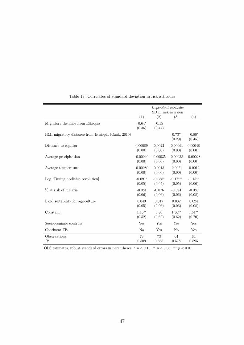
Table 13: Correlates of standard deviation in risk attitudes

Dependent variable:SD in risk aversion

(1) (2) (3) (4)

Migratory distance from Ethiopia -0.64∗ -0.15(0.36) (0.47)

HMI migratory distance from Ethiopia (Ozak, 2010) -0.73∗∗ -0.80∗(0.29) (0.45)

Distance to equator 0.00089 0.0022 -0.00061 0.00048(0.00) (0.00) (0.00) (0.00)

Average precipitation -0.00040 -0.00035 -0.00038 -0.00028(0.00) (0.00) (0.00) (0.00)

Average temperature -0.00080 0.0013 -0.0021 -0.0012(0.00) (0.00) (0.00) (0.00)

Log [Timing neolithic revolution] -0.091∗ -0.088∗ -0.17∗∗∗ -0.15∗∗(0.05) (0.05) (0.05) (0.06)

% at risk of malaria -0.081 -0.076 -0.094 -0.080(0.06) (0.06) (0.06) (0.08)

Land suitability for agriculture 0.043 0.017 0.032 0.024(0.05) (0.06) (0.06) (0.08)

Constant 1.16∗∗ 0.80 1.36∗∗ 1.51∗∗(0.52) (0.62) (0.62) (0.70)

Socioeconimic controls Yes Yes Yes Yes

Continent FE No Yes No Yes

Observations 73 73 64 64R2 0.509 0.568 0.578 0.595

OLS estimates, robust standard errors in parentheses. ∗ p < 0.10, ∗∗ p < 0.05, ∗∗∗ p < 0.01.

47

BWACMR

GHAKEN

MWI

NGA

RWA

TZA

UGA

ZAF

ZWE

DZA

EGY

IRN

IRQISR

JOR

MAR

SAU AUTCHE

CZE

DEUESP

EST

FIN

FRA

GEO

GRC

HRV

HUN

ITA

KAZ

LTUMDA

NLD

POLROU

RUS

SWETUR

UKR

CHN

KHM

KOR

THA

VNM

AFG

BGD

INDPAKARG

BOLBRA

CHLCOLCRI

GTM

MEX

NICPER

VEN

CAN

USA

.7.8

.91

1.1

1.2

SD in

risk

ave

rsio

n

0 .05 .1 .15 .2 .25Mobility index-based migratory distance from Ethiopia

Sub-Saharan Africa ME & North Africa EU & Central Asia East AsiaSouth Asia South America North America

Preference heterogeneity and migratory distance to Ethiopia

Figure 5: Migratory distance from South Africa and preference heterogeneity

F Relationship Between Risk Preferences and Out-

comes

F.1 Average Risk Aversion and Riskiness of the Environment

Table 14 presents correlations between the average level of risk aversion in a givencountry and the riskiness of the environment, as proxied for by life expectancy atbirth, HIV prevalence, the traffic death rate, a poverty ratio, the Gini index, thefraction of income that goes to the top 10%, and a labor protection index. Also seeFalk et al. (2015a).

48

Tab

le14:Average

risk

taking

andriskinessof

theenvironm

ent

Dep

endent

variab

le:

Healthrisks

Econo

mic

risks

Life

expe

ctan

cyLo

g[H

IVprevalence]

Traffi

cdeathrate

Poverty

ratio

Giniind

exIncomeshareof

top10%

Labo

rprotection

(1)

(2)

(3)

(4)

(5)

(6)

(7)

(8)

(9)

(10)

(11)

(12)

(13)

(14)

Risktaking

-12.3∗

∗∗-9.69∗

∗∗1.96

∗∗1.78

∗∗9.37

∗∗∗

7.66

∗∗∗

14.0

∗8.90

∗∗9.45

∗∗9.58

∗∗9.59

∗∗9.00

∗∗-0.24∗

∗∗-0.21∗

∗

(4.01)

(3.34)

(0.74)

(0.74)

(2.78)

(2.88)

(7.83)

(4.23)

(4.46)

(4.53)

(3.94)

(4.20)

(0.08)

(0.08)

Log[G

DP

p/cPPP]

4.32

∗∗∗

-0.30∗

∗∗-2.90∗

∗∗-11.1∗

∗∗0.35

-1.71∗

∗∗0.01

5(0.34)

(0.10)

(0.39)

(1.23)

(1.14)

(0.44)

(0.02)

Con

stan

t70

.6∗∗

∗34

.7∗∗

∗-0.86∗

∗∗1.62

∗15

.3∗∗

∗39

.5∗∗

∗13

.3∗∗

∗96

.8∗∗

∗41

.2∗∗

∗38

.6∗∗

∗31

.0∗∗

∗45

.2∗∗

∗0.49

∗∗∗

0.37

∗∗∗

(0.96)

(3.13)

(0.17)

(0.89)

(0.92)

(3.49)

(2.08)

(9.96)

(1.23)

(8.74)

(0.86)

(3.97)

(0.02)

(0.14)

Observation

s76

7669

6974

7450

5052

5268

6856

56R

20.15

80.69

20.15

00.24

50.11

10.40

30.07

70.69

20.09

10.09

30.12

90.25

20.13

50.14

8

OLS

estimates,r

obuststan

dard

errors

inpa

rentheses.

Labo

rprotection

isan

indextakenfrom

Boteroet

al.(20

04).

∗p<

0.10

,∗∗p<

0.05

,∗∗∗p<

0.01

.

49

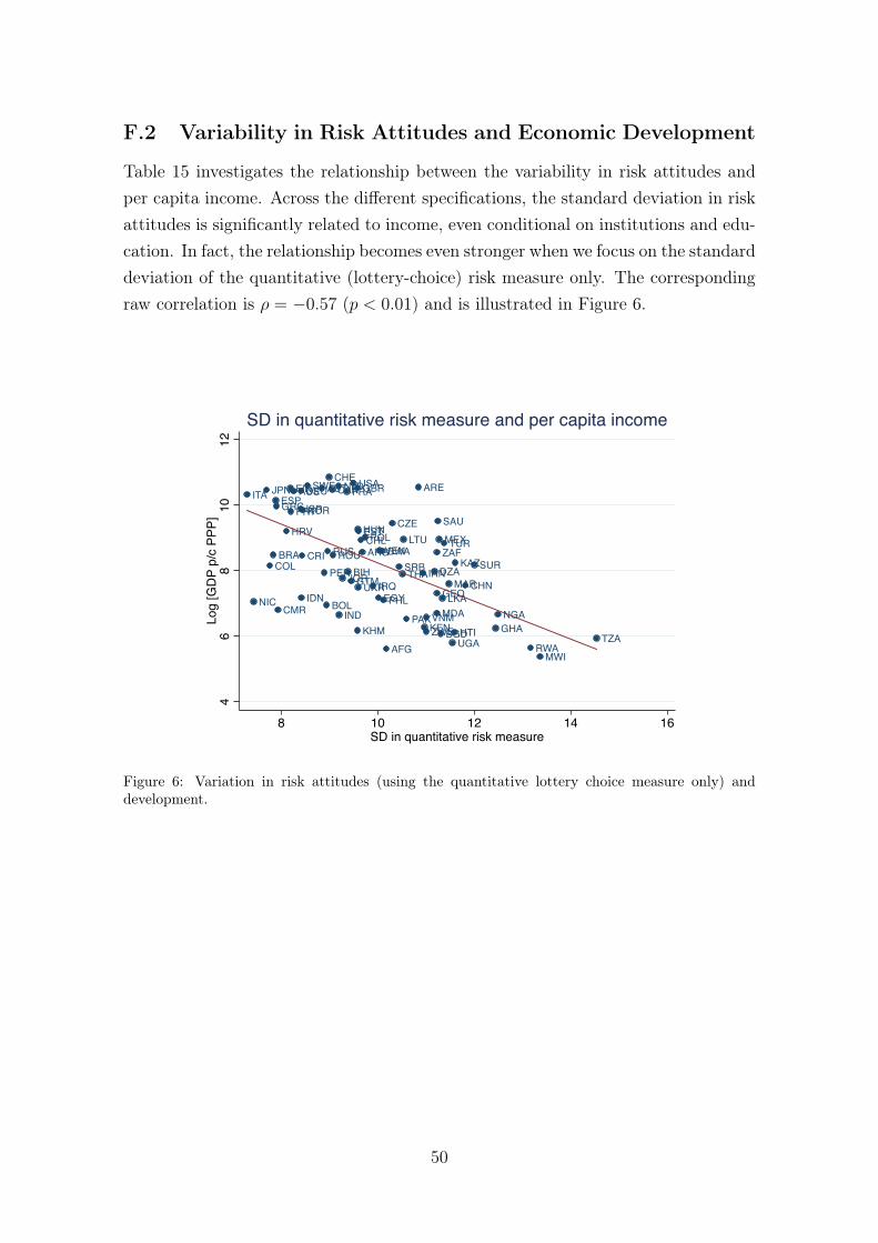
F.2 Variability in Risk Attitudes and Economic Development

Table 15 investigates the relationship between the variability in risk attitudes andper capita income. Across the different specifications, the standard deviation in riskattitudes is significantly related to income, even conditional on institutions and edu-cation. In fact, the relationship becomes even stronger when we focus on the standarddeviation of the quantitative (lottery-choice) risk measure only. The correspondingraw correlation is ρ = −0.57 (p < 0.01) and is illustrated in Figure 6.

AFG

ARE

ARG

AUS AUT

BGD

BIH

BOL

BRA BWA

CANCHE

CHL

CHN

CMR

COLCRI

CZE

DEU

DZA

EGY

ESP

EST

FIN FRAGBR

GEO

GHA

GRC

GTM

HRV

HTI

HUN

IDNIND

IRNIRQ

ISRITA

JOR

JPN

KAZ

KENKHM

KOR

LKA

LTU

MAR

MDA

MEX

MWI

NGANIC

NLD

PAK

PER

PHL

POL

PRT

ROURUS

RWA

SAU

SRB SUR

SWE

THA

TUR

TZAUGA

UKR

USA

VEN

VNM

ZAF

ZWE

46

810

12Lo

g [G

DP p

/c P

PP]

8 10 12 14 16SD in quantitative risk measure

SD in quantitative risk measure and per capita income

Figure 6: Variation in risk attitudes (using the quantitative lottery choice measure only) anddevelopment.

50

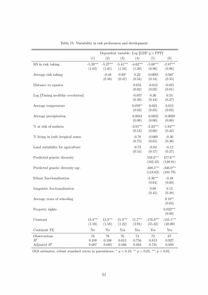
Table 15: Variability in risk preferences and development

Dependent variable: Log [GDP p/c PPP](1) (2) (3) (4) (5) (6)

SD in risk taking -5.39∗∗∗ -5.27∗∗∗ -5.41∗∗∗ -4.62∗∗∗ -5.00∗∗∗ -2.87∗∗∗(1.62) (1.61) (1.34) (1.20) (0.96) (0.86)

Average risk taking -0.48 0.89∗ 0.22 -0.0085 0.087(0.56) (0.47) (0.34) (0.34) (0.35)

Distance to equator 0.034 -0.012 -0.021(0.02) (0.02) (0.01)

Log [Timing neolithic revolution] -0.057 0.36 0.24(0.39) (0.44) (0.27)

Average temperature 0.059∗∗ 0.023 0.015(0.03) (0.03) (0.02)

Average precipitation 0.0044 -0.0045 -0.0038(0.00) (0.00) (0.00)

% at risk of malaria -2.01∗∗∗ -2.23∗∗∗ -1.64∗∗∗(0.54) (0.60) (0.42)

% living in (sub-)tropical zones -0.78 -0.069 -0.36(0.73) (0.65) (0.46)

Land suitability for agriculture -0.73 -0.82 -0.12(0.54) (0.57) (0.37)

Predicted genetic diversity 559.2∗∗∗ 477.6∗∗∗(162.10) (138.91)

Predicted genetic diversity sqr. -408.5∗∗∗ -346.0∗∗∗(118.63) (101.79)

Ethnic fractionalization -2.36∗∗∗ -0.48(0.64) (0.60)

Linguistic fractionalization 0.68 0.13(0.45) (0.48)

Average years of schooling 0.10∗∗(0.04)

Property rights 0.022∗∗∗(0.00)

Constant 13.4∗∗∗ 13.3∗∗∗ 15.3∗∗∗ 11.7∗∗∗ -176.8∗∗∗ -155.1∗∗∗(1.58) (1.58) (1.22) (3.91) (55.32) (48.00)

Continent FE No No Yes Yes Yes Yes

Observations 76 76 76 74 72 67R2 0.100 0.108 0.613 0.756 0.813 0.927Adjusted R2 0.087 0.083 0.566 0.693 0.745 0.893

OLS estimates, robust standard errors in parentheses. ∗ p < 0.10, ∗∗ p < 0.05, ∗∗∗ p < 0.01.

51

G Definitions and Data Sources of Main Variables

G.1 Explanatory Variables

Fst and Nei genetic distance. Genetic distance between contemporary popula-tions, taken from Spolaore and Wacziarg (2009).

Linguistic distance. Weighted linguistic distance between contemporary popula-tions. Derived from the Ethnologue project data, taking into account all languageswhich are spoken by at least 5% of the population in a given country.

Predicted migratory distance. Predicted migratory distance between two coun-tries’ capitals, along a land-restricted way through five intermediate waypoints (oneon each continent). Taken from Ashraf and Galor (2013b).

HMI migratory distance. Walking time between two countries’ capitals in years,taking into account topographic, climatic, and terrain conditions, as well as humanbiological abilities. Data from Özak (2010).

G.2 Covariates and Outcome Variables

Average age, proportion female, standard deviation age, gender hetero-geneity index, standard deviation of household income. Computed fromGallup’s sociodemographic background data. Gender heterogeneity is computed as(2× proportion female − 1)2.

Religious and linguistic fractionalization. Indices due to Alesina et al. (2003)capturing the probability that two randomly selected individuals from the samecountry will be from different religious / linguistic groups.

Percentage of European descent. Constructed from the “World Migration Ma-trix” of Putterman and Weil (2010).

Contemporary national GDP per capita. Average annual GDP per capita overthe period 2001 – 2010, in 2005US$. Source: World Bank Development Indicators.

Democracy index. Index that quanties the extent of institutionalized democracy,as reported in the Polity IV dataset. Average from 2001 to 2010.

52

Property rights. This factor scores the degree to which a country’s laws protectprivate property rights and the degree to which its government enforces those laws.It also accounts for the possibility that private property will be expropriated. Inaddition, it analyzes the independence of the judiciary, the existence of corruptionwithin the judiciary, and the ability of individuals and businesses to enforce contracts.Average 2001-2010, taken from the Quality of Government dataset, http://www.qogdata.pol.gu.se/codebook/codebook_basic_30aug13.pdf.

Colonial relationship dummies. Taken from the CEPII Geodist database athttp://www.cepii.fr/CEPII/en/bdd_modele/presentation.asp?id=6.

Geodesic distance, contiguity, longitude, latitude, area, 1 if landlockedTaken from CEPII GeoDist database. The longitudinal distance between two coun-tries is computed as

Longitudinal distance = min{|longitudei−longitudej|, 360−|longitudei|−|longitudej|}

Suitability for agriculture. Index of the suitability of land for agriculture basedon ecological indicators of climate suitability for cultivation, such as growing degreedays and the ratio of actual to potential evapotranspiration, as well as ecologicalindicators of soil suitability for cultivation, such as soil carbon density and soil pH,taken from Michalopoulosa (2012).

Percentage of arable land. Fraction of land within a country which is arable,taken from the World Bank Development Indicators.

Terrain roughness. Degree of terrain roughness of a country, taken from Ashrafand Galor (2013b). Data originally based on geospatial undulation data reported bythe G-ECON project (Nordhaus, 2006).

Mean and standard deviation of elevation. Mean elevation in km above sea,taken from Ashraf and Galor (2013b). Data originally based on geospatial elevationdata reported by the G-ECON project (Nordhaus, 2006).

Timing of the neolithic transition. The number of thousand years elapsed,until the year 2000, since the majority of the population residing within a country’smodern nationalw borders began practicing sedentary agriculture as the primarymode of subsistence. The measure is weighted within each country, where the weightrepresents the fraction of the year 2000 population (of the country for which the

53

measure is being computed) that can trace its ancestral origins to the given countryin the year 1500. Measure taken from Ashraf and Galor (2013b).

Precipitation. Average monthly precipitation of a country in mm per month,1961-1990, taken from Ashraf and Galor (2013b). Data originally based on geospatialaverage monthly precipitation data for this period reported by the G-ECON project(Nordhaus, 2006).

Temperature. Average monthly temperature of a country in degree Celsius, 1961-1990, taken from Ashraf and Galor (2013b). Data originally based on geospatialaverage monthly temperature data for this period reported by the G-ECON project(Nordhaus, 2006).

Life expectancy. Life expectancy at birth, average 2001–2010. Taken from theWorld Bank Indicators.

Percentage at risk of contracting malaria. The percentage of population inregions of high malaria risk (as of 1994), multiplied by the proportion of national casesinvolving the fatal species of the malaria pathogen, P. falciparum. This variable wasoriginally constructed by Gallup et al. (2000) and is part of Columbia University’sEarth Institute data set on malaria.

Freight cost of surface transport Cost of 1,000 kg of unspecified freight trans-ported over sea or land with no special handling, taken from Spolaore and Wacziarg(2009). Data originally retrieved from http://www4.importexportwizard.com/.

Distance to nearest waterway. The distance, in thousands of km, from a GISgrid cell to the nearest ice-free coastline or sea-navigable river, averaged across thegrid cells of a country. Source: Ashraf and Galor (2013b), originally constructed byGallup et al. (1999).

Executive constraints. The 1960-2000 mean of an index (1-7) that quantifies theextent of institutionalized conatrsints on the executive, as reported in the Polity IVdata set. Data taken from Ashraf and Galor (2013b).

Average years of schooling. The mean over the 2000-2010 time period, of the5-yearly figure, reported by Barro and Lee (2012), on average years of schoolingamongst the population aged 25 and over.

54

Population. Average 2001-2010, taken from the World Bank Development Indica-tors.

Linguistic diversity. Computed akin to linguistic and religious distance indicesby matching a country with itself.

HIV prevalence. Primary data taken from Unicef. Missings replaced by datafrom most recent available period of the World Bank Development Indicators.

Traffic death rate. Traffic deaths per 1,000 population, estimate of the WorldHealth Organization.

Poverty headcount ratio. Fraction of the population living on less than $2 perday, average 2001-2010. Taken from World Bank Development Indicators.

Gini index. Average 2001-2010. Taken from World Bank Development Indicators.

Income share of top 10%. Average 2001-2010. Taken from World Bank Devel-opment Indicators.

Labor protection index. Index capturing the rigidity of employment laws byBotero et al. (2004). Includes data on employment, collective relations, and socialsecurity laws and measures legal worker protection.

55