-------- CHAPTER 19

The Analytical Stormwater Management Model (ASWMM)

Yiping Guo and Barry J. Adams

This chapter outlines the methodology and procedures used in the development and verification cfthe Analytical Stonnwater Management Model (ASWMM). ASWMM is a collection of analytical expressions relating the runoff character­istics and storm water detention pond performance measures of urban catchments directly to the rainfail statistics and system parameters. These analytical expressiom are derived from the simplified mathematical representation of the hydrologic and processes involved. The input rainfall event character­istics are treateJ as exponentially distributed random variables. Preliminary resting and indicate that the ASWMM results are generally in close agreement with those generated fi·om the U.S. EPA SWMiv1 model. The use of ASWMM is therefore proposed for the planning and design of urban storm water management facUlties.

19.1 Introduction

The Stormwater 1\,·ianagement Model (SWMM) (Huber and Dkkimon, 1988) has been widely used in the planning and design of stormwatcr management facilities for urban areas. Continuous simulation using S\lilMM 01·other numerical

Guo, Y. and B.J. Adams. 1999. "The Analytical Stormwater Management Model (ASWMM)." Journal of Water Management Modeling R204-19. doi: I 0.14796/JWMM.R204-19. ©CHI 1999 www.chijournal.org ISSN: 2292-6062 (Formerly in New Applications in Modeling Urban Water Systems. ISBN: 0-9697422-9-0)

347

348 The Analytical Storm water Management Alodel (ASWMM)

hydrologic models is performed to predict the volumes and peak discharge rates of runoff from urban catchments associated with certain return periods, and the performance of storm water quantity and quality control facilities.

The objective of this chapter is to outline the development and testing of a set of mathematical expressions which can be used for the determination of the runoff event volume and peak discharge rate from urban catchments associated with certain return periods, and the runoff quantity and quality control perfor­mance provided by a detention pond servicing an urban catchment. These expressions, collectively referred to as the Analytical Stormwater Management Model, or ASWMM, relate statistical urban drainage system perfonnance measures directly to meteorological parameters, system properties and design variables. Compared with numerical hydrologic models, ASWMM is computationally more efficient and can be used as an alternative to numerical hydroiogic models in the planning and design of stormwater management facilities for urban areas.

The approach taken for the development of ASWMM can be briefly summarized as follows. Firstly, statistical analyses oflong-term rainfall records are performed, leading to the determination onhe probability density functions (pdfs) ofrainfaH event characteristics. Secondly, the hydrologic and hydraulic processes taking place on an urban catchment are mathematically represented on an event-by-event basis, establishing the functional relationship berween the input rainfall characteristics and the output nmoff characteristics. Thirdly, the pdfs of mnoff characteristics are derived from those of the input rainfall characteristics and the functional relationships between the input and output variables. The derivation process for the determination of the desired pdfs follows the principle of derived probability distribution theory (Benjanlin and Cornell, 1970). Details of the development and verification processes, and some of the iengthy analytical solutions are contained in Guo (1998). This chapter serves as an introduction to, and an outline of, the proposed methodology.

19.2 Statistical Analysis of Rainfall Data

Urban catchments are often small in size, ranging from several hectares to a few hundred hectares. It is assumed that rainfall on catchments of such size is adequately described by a representative point rainfall. In the statistical analysis of historical rainfall records, a continuous rainfall series is first divided into discrete rainfall events. The criterion for distinguishing between events is a minimum time pedod without rainfall (termed the minimum interevent time def1nition - IETD). Rainfall periods separated by a time interval longer than the IETD are considered to be separate rainfall events. Once this distinction is made, a point rainfall series may be divided into discrete events and the characteristics of these events may be statistically analyzed.

19.2 Statistical Analysis ofRairifali Data 349

The choice ofthe IETD is governed by the intended application. The results ofthis research may be applied to urban catchments with a response time (such as the time of concentration) of the order of half an hour to two or three hours. To ensure a one-to-one correspondence between rainfall a.'1d runoff events on these catchments, the IETD for rainfall event separation should be greater than the catchment response time. On the other hand, if the IETD is too long, consecutive rainfall events are considered to belong to the same event. Thus, an IETD of about six hours may be considered appropriate for the analysis of typical urban catchment'>. Details on meteorological data analysis for urban drainage system design and the proper choice ofthe IETD can be found in Adams et a1. (986), Eagieson (1972), Fraser (1982), Howard (1976), and Restrepo-Posada and Eagleson (1982).

Each rainfall event is characterized by its rainfall volume (v), rainfall duration (t). and interevcnt time (b), The historical rainfan record can then be viewed as comprising a time series for each of the above characteristics \;chich individuaHy may be submitted to a n'equency analysis. Histograms of the time series are and probability density functions are fitted to the histograms. An average annual !lumber of storm events can also be obtained from these statistical It has been found that exponential pdfs often fit such

1972; Howard, 1976; Adams et aJ., 1984, ,,,,,,~,,,.,~t of ASWMM, the exponential distributions for

in Table 19.1 are considered appropriate. In Table 19.1. t, and bare the average event volume, average event duration, and average interevent time of the rainfall record, respectively. As an example, the

historical rainfall record of Pearson International Airport in Toronto, Canada \vas and the resulting statistics are induded in Table 19.1.

functions of rainfall characteristics and rainfall statistics for Toronto, Canada (IETD = 6h).

Exponential pdf

Volume, l' (mm)

Distribution j'aramcter

Toronto Statistics

v = 9.43mm

___ H~~ ___ "~"""" .......... _ .. _ ... _ ....... ~ .... ~ ______ ...... ~ ... _ .... ~_ .. _ .. __ • ___ _

Durnt10n, t (11) t == 7. 73hours

--~ ..... -..• - .. - ......... --.... - .............. - ... --.. ----.------- -----lntcrevcnt Time, b (h) f B (ll) == \11 exp( -llIb) 1

\jI== b

b = 103.1hours

Average Annual Number of Rainfall Events, () 57.2

Average Annual Rainfall Volume 550mm

350 The Analytical Storm water Management Model (ASWMlvf)

19.3 Rainfall-Runoff Transformation

The rainfall-runoff transformation discussed in this section establishes the relationships between the input rainfall event characteristics and the output runoff event characteristics. Once these functional relationships are established, the probability distributions of those runoff characteristics, which are of interest in planning and design, can be established using derived probability distribution theory.

A runoff event as considered here is characterized by runoff event voiume, runoff event duration and peak discharge rate. The calcuiated runoff event volume is the difference behveen the volume of the input rainfall event and the total volume of hydrologic losses. For the purposes of hydrologic modeling, interception and depression storage losses are often lumped together. The same approach is taken in the development of ASWMM; thus, depression storage losses hereinafter include losses due to interception. Furthermore, in the devel­opment of ASWMM, it is assumed that surface depressions are filled before any runoff occurs for each rainfaJI event, and that the dry period that follows is always long enough so that water accumulated in the depression storage areas is completely evaporated and surface depressions are fully available at the begin­ning of each rainfall event.

The total infiltration losses within a runoff event are considered to be the combination of two parts; namely, losses due to initial wetting of the soil and losses as a result of infiltration at a constant rate, fe' throughout the duration of the runoff event. That is:

where:

S mf = S iw + f c t (19.1)

the maximum possible infiltration loss volume during a rainfall event of duration t; the initial soil wetting infiltration volume which is assumed to be the same for all rainfall events;

t~ == the ultimate infiltration capacity ofthe catchment soils.

It is shown in Guo (1998) that the value of Siw can be estimated from the infiltration parameters ofthe soil and meteorological parameters of the region.

Similar to many numerical hydrologic models, in calculating the total rainfall losses, the urban catchment is divided into impervious and pervious areas. For impervious areas, the infiltration loss is assumed to be zero and the input rainfall volume is totally converted to runoff volume after filling the impervious area depression storage, Sdi' in mm.

19.4 Runo.tfEvent Volume and Peak Discharge Rate 35J

for pervious areas, the input rainfall volume fills the pervious area depres­sion storage, SdP' and infilh'ates into the soil; the rainfall voh.une remaining after the filling of depression storage and infiltration into the soil becomes surface runoff. The units ofSdi and Sdp are mm of water over the entire impervious area and the entire pervious area, respectively. The duration ofinfiltration is essen­tially the same as the rainfall duration, because it takes little time for runoff from the pervious surfaces to reach the impervious portions of the catchment or the sewer system. Thus, infiltration on the pervious portions of an urban catchment ceases soon after the end of the rainfall event. The maximum possible infiltration losses within the rainfall event are determined using Equation 19.1. To simplify expressions, the sum ofSar and Siw is denoted as Sil hereafter, and is referred to as the pervious area initial losses.

The overall runoff generation of the urban catchment is the area··weighted combination of the runoff from the pervious and impervious portions of the catchment. In an urban catchment, Sdi is usually less than Sdp' Therefore, if v is less than SCi' then v must be less than (Sil + fct), since fc and t are both positive. If the ii-action of impervious area of the urban catchment is h (for hardened surface fraction), then combining the runoff volumes from impervious and pervious areas of an urban catchment gives the foHovv-ing equation:

, V sSdi

, Sill <vsSii +fc t

, v>Si\+fc t (19.2)

where Sd = hSdi -'- (1 - h)SH' is the area-weighted depression storage of the imperviotL<; areas .md the initial losses of the pervious areas of the urban catchment. Detailed derivations of Equatiol1 19.2 can be found in Guo (1998).

19.4 Runoff Event Volume and Peak Discharge Rate

Equation 19.2 dC5cribes the functional relationship betvveen dependent random variable vr and indepencientrandom variables \' and t. The probability distribution and the expecteu value ofvr were derived using derived probability distIibution theory and this fhnctional relationship (Guo, 1998). The derived probability distribution of v r is lengthy and is not suitable for hand calculations. It is not included in this chapter but can be found in Guo (1998). However, the expected value of vr per rainfall event has a simple form:

h 1..(1-- h) E(v r ) =: -exp(-sSdJ + exp(-t::;Si')

t::; t::;(t::;fc + A) , (19.3)

352 The Analytical Storm water Management lv/odel (ASWMM)

The average annual runoff volume is simply the product of E(vr) and the average annual number of rainfall events 9.

The rising and recession shapes of runoff hydrographs can often be approximated by triangles. The time base of the hydrograph, or the duration of the runoff event, is derived through the use of the catchment time of concentra­tion. Thetecm time of concentration, denoted as is defined as the time required for runoff to travel from the most remote portion of the catchment to its outlet or design point. The duration of the runoff event can then be estimated as t + tc; Le. the duration of the rainfall event plus the catchment time of concentration. This can be drawn from the observation that runoff at the outlet starts at L~e beginning of the corresponding rainfall event if the delay caused by the time needed to fill the depressions ofthe catchment is negligible; and that it takes time tc for the last drop of water falling on the most remote part of the catchment to reach the outlet.

The catchment time of concentration is treated as a {:onstant independent of rainfall characteristics for the detennination offlood frequencies. In this regard, the catchment time of concentration can be viewed as a parameter combining the effects of catchment slope, roughness, length, shape and topology. The peak discharge rate, Qp' of a triangular hydrograph with runoff volume vr' and time bac;e (t + t,) determined from the hydrograph geometry:

Q :::: 2vr_ P t' t T C

(19.4)

It is noted that the above expression for peak discharge rate is independent of the ratio of the time to peak to the time base ofthe hydrograph. Arguably, Equation 19.4 may provide good estimates of peak discharge rates for some runoff events, but poor estimates for other events. The overall acceptability of invoking the triangular hydrograph assumption in estimating peak discharge rate may be justified when the interest is in the detennination of the exceedance probability of peak discharge rates from thousands of independent runoff events. The reasonableness of this assumption is tested when the analytically derived results are compared with those from long-term continuous simulation Jater in this chapter.

Using the functional relationship described in Equation 19.4, Guo (1998) derived the peak discharge rate exceedance probability per rainfall event which can be used to analytically determine the peak discharge rates associated with certain return periods. The derived peak discharge rate exceedance probability expressions are lengthy and are not suitable for hand calculations. Details of the analytical expressions can be found in Guo (1998) where they are implemented in computer spreadsheets.

19.5 Stornnvater Quality Control Analyses 353

19.5 Stormwater Quality Control Analyses

A common scenario in urban stonnwater quality control is that runoff from a contributing catchment is directed to a detention pond, and outflow from the pond is discharged to a downstream receiving water. Whenever the pond is full, inflow in excess of the maximum pond outflow rate, which corresponds to the orifice flow under the maximum head, is spilled upstream of the pond or through a spillway constructed as a part of the pond. Clearly, spills upstream ofthe pond receive no treatment at all, and it can be assumed that spills through the spillway ofthe pond receive essentially no treatment as well, because ofthe short detention time provided by the pond under overflow conditions.

Two perfonnance measures, i.e. flow capture efficiency and average detention time, can be used in evaluating the long-term average pollutant removal effectiveness of storm water detention ponds.

19.5.1 Flow Capture Efficiency

The flow , CR' provided by a detention pond in the above scenario, is defined as the traction of runoff volume captured by the detention pond, excluding the spill volume. In accordance with the event-ba<;ed analysis method, the flow capture efficiency can be calculated as follows:

(19.5)

eXi}ecteovalue ofthe spill voiume, P, perrainfaH event, in mm over the and is given by Equation 19.3.

Spills fhml a stornnovater detention pond occur due to two primary cau.'';cs. On one hand, spilb may occur because the pond storage volume is not suff1cient to contain the nmotl event volume from the catchment, even though the pond storage volume is entirely available at the beginning of the runoff event. On the other hand, spills may occur because part of the pond storage capacity is still occupied by nmoff f1°om previous events at the beginning of a runoff event. This IS to of successive storms and occurs if the outflow

is too small for outflow to cease between successive runoff events. spi!l~ between the two causes provides insight into the impact on spill volumes of the two pond design variables, namely, storage volume and outflow rate.

Hereafter, fi'om a stonnwater detention pond resulting from the small storage volume effect, neglecting the carryover effect of successive runoff events, are referred to as event spills, while spills due mainly to the carryover effect of successive runoff events are termed carryover spills. The volume of the

The Analytical Storm water Management Model (ASWMl.1)

event spill resulting from a rainfall event is denoted P ; and the volume of the e

354

carryover spill which occurs during a rainfall event as a result of the carryover effect of previous rainfall events is denoted Pc'

The sum ofPe and Pc is the total spill volume P from the input ofarainfall event to a pond which mayor may not be empty at the beginning of the rainfall event because of previous events, and

E(P) == E(Pe ) + E(Pc ) (19.6)

where E(Pe ) and E(Pc) are the expected values ofP!! and Pc per rainfall event, respectively. The annual average event spill volume, annual average carryover spill volume, and annual average spill volume can be calculated as the product ofthe respective expected value and the annual avea-age number of rainfall events.

The expressions for E(Pe) and E(Pc) are derived in Guo (1998). These expressions are lengthy and are not included here. Computer spreadsheet~ are developed in Guo (1998) incorporating the analyticai expressions for E(P e) al1d E(P c), These spreadsheets can be used for the determination of now capture efficiencies.

19.5.2 Average Detention Time

F or each runoff event, regardless ofthe mixing regime in the detention pond, the volume-weighted average detention time provided by the pond is the horizontal distance between the centroids of the inflmv and outflow hydrographs. This horizontal distance can be approximated by the distance between the mid-points ofthe time bases of the inflow and outflow hydrographs. The storage-discharge relationship ofthe pond may be approximated as a linear function, i.e.

Q= SQ a

(19.7)

where SQ (in mm over the contributing catchment) is the pond storage volume corresponding to outflow rate Q (in mmlh); and a (in h) is the proportionality constant with a dimension of time. The storage-discharge relationships of storm water quality control ponds are usually not exactly linear. For the estima­tion of average detention time, a in Equation 19.7 can be estimated from the average slope of the real storage-discharge curve.

With these approximations, it was shown (Guo, 1998) that, for any single event, the average detention time td is a function of the catchment time of concentration tc' pond design parameter a, and interevent time h. Both tc and a are constants, while b is a random variable with an exponential pdf as presented in Table 19.1. The overall voiume-weighted average td was derived as the expected value oftd and is given as foHows:

19.6 Flood Control Ana{vses

E(t a) = exp( -\lite) [1- exp(- 2alji)] 2\ji

355

(19.8)

Equation 19.8 can be used to estimate the overall volume-weighted average detention time provided by a detention pond servicing an urban catchment. Based on Equation 19.8, it can be concluded that as a increases, the average detention time increases; while as tc increases, the average detention time decreases. Furthermore, Equation 19.8 shows that the overall volume-weighted average detention time is also affected by the meteorological parameter '1'.

19.6 Flood Control Analyses

Continuous probability or continuous return period criteria are often specified for the sizing of urban flood detention facilities. These criteria require that for aU storm events up to and including the most severe event, peak discharges for the developed condition \vith flood control in place shaH not exceed peak discharges under existing conditions (Walesh, 1989). The design stonn approach often represents the state-ot:'the-art for designing flood control detention facili­ties to continuous probability criteria. This involves the use of multiple design storms which are usually developed and 11 regulatory agency of the jurisdiction.

Inherent in the design storm based approach is the assumption that the return period design storm is to the return of the peak rate from the catch.rnent tlum the input storm, and the consequent outflow rate from the flood control It is \vell~known this basic is t1awed Marsalek, 1978; Wenzel and Voorhees, 1978, 1979; J 982; Robinson and James, 1 Adams and ,u',,,,,,,-n 1986).

An alternative approach which overcomes the shortcomings of the storm is continuous simub.tion. This involves the use of long-term historical records together with a simulation model to evaluate the simulated historical response of a proposed system. The design is modH1ed so as to an acceptable statistical performance of the system, consistent the specified continuous criteria for flood controL Given a record of sufficient length and an adequate simulation model, the statistics ofthe continu­ous simulation model output, and hence the statistics ofthe system perfonnance, are deemed to be reliable. The disadvantage of the continuous simulation approach is that it may be costly and awkward because of the data assembly and analysis efforts required. As a result, continuous simulation has not been commonly used in sizing flood control detention facilities.

356 The Analytical Storm water Management Model (ASWMM)

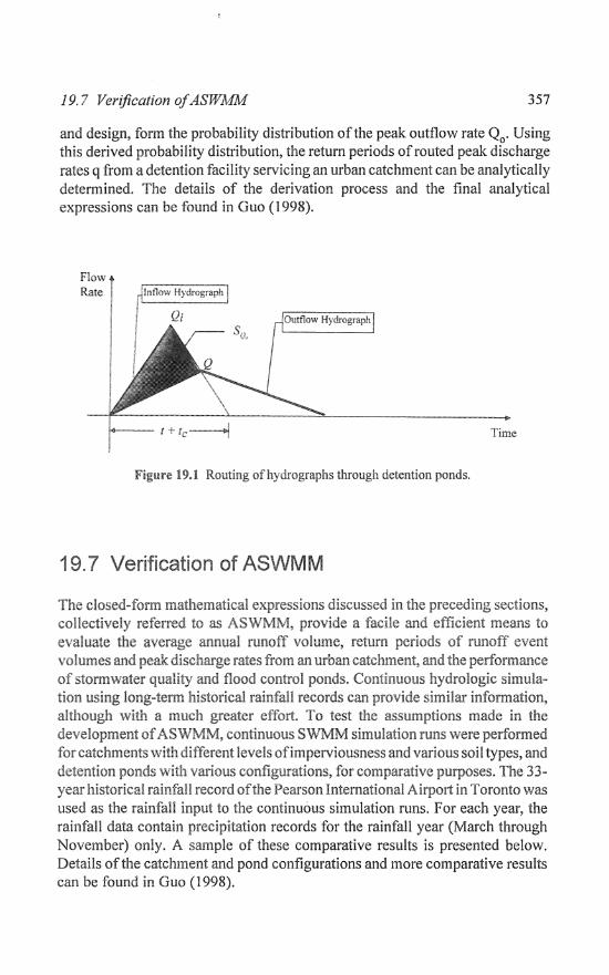
Analytical procedures were developed to approximate the continuous simulation modeling approach for the sizing of detention facilities for flood control purposes (Guo, 1998). With a triangular inflow hydrograph and the assumptions that at the start of any runoff event, the detention facility is empty. and that the outflow hydrographs have a linear rising lilItb, the routing of the hydrograph through a detention facility for each runoff event is represented L'1 Figure 19.1.

As shown in Figure 19.1, the time base of the inflow hydrograph is t + ie' where t is the duration of the causal rainfaU event and tc is the catcP.ment time of concentration. The outflow occurs immediately after the start of the inflow hydrograph. The outflow hydrograph intersects the inflow hydrograph at the peak ofthe outflow hydrograph along the recession limb of the inflow hydrograph, since the detention volume is specifically designed to avoid uncontrolled spiHs. 'I11e volume of the runoff event, vr' in mm of "water over the catchment, entering the detention facUity is equal to the area enclosed by the inflow hydrograph. The shaded area in Figure 19.1, denoted SQ" is equal to the maximum storage volume utilized during the passage of the runoff event. Hence, the peak outflow rate, Q", 1S the discharge rate of the detention facility at storage volume SQG'

From Figure 19.1, it can be seen that:

SQ =~(Q"-Q Xt+t)" o 2 I O. C (19.9)

where Q j is the peak inflow rate. Q j and Qo are both in the units of mm/h, is in units ofmm, and tand tc3rc both inh. Rearranging Equation 19.9, and noting that

the following is obtained:

2(v r -SQ ) Qo =: •

t + tc (19.10)

The storage-discharge relationship of a detention facility is described by a table of ordered pairs of storage volume and discharge rate values. Each pair of these values is denoted (Sq, q), where Sq is the storage volume of the detention facility at which the routed discharge rate from the facility equals the given value q. Utilizing the functional relationship between dependent random variable Qo

and independent random variables Vr and t as described in Equation 19.10, Guo (1998) derived an analytical expression for the exceedance probability P[Q(l>q] as a function of contributing catchment hydrologic parameters, meteorological parameters, and q and the corresponding Sq values. The ordered combinations of P[Qo>q] for all the possible discrete values of q, that are of interest in planning

19.7 Verification ojASWAflvi 357

and design, form the probability distribution of the peak outflow rate Qo' Using this derived probability distribution, the return periods of routed peak discharge rates q fi'om a detention facility servicing an urban catchment can be analytically determined. The details of the derivation process and the final analytical expressions can be found in Guo (1998).

Flow Rate

ji'igure 19.1 Routing of hydro graphs through detention ponds.

Time

19.7 Verification of ASWMM

TIle dosed-form mathematical expressions discussed in the preceding sections, collectively referred to as AS\VTv1M, provide a facile and efficient means to c"valuate the average annual runoff volu.me, retum periods of runoff event

and pea.l( discharge rates from an urban catchrnent, and the perfOrmtU1Ce of stormwater quality and flood control ponds. hydrologic simula­tion using long-term historical records can provide similar information, although \-vith a much greater effort. To test the assumptions made in the development continuous SWMM simulation runs were performed for catchments with different levels ofimperviousness and various soil types, and

\vith various configurations, for purposes. The 33-year historical rainfall record ofthe Pearson International Airport in Toronto was used a.<; the rainfall input to the continuous simulation runs. For each year, the rainfall data contain precipitation records for the rainfall year (March through November) only. A sample of these comparative results is presented below. Details of the catchment and pond configurations and more comparative results can be found in Guo (1998).

358 The Analytical Stornn1later Management Model (ASWMA1)

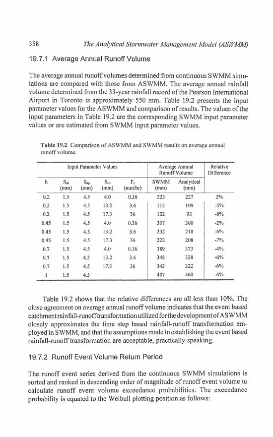
19.7.1 Average Annual Runoff Volume

The average annual nmoffvolumes determined from continuous SWMM simu­lations are compared with those from ASWMM. The average annual rainfall volume determined from the 33-yc31' rainfan record afthe Pearson international Airport in Toronto is approximately 550 mm. Table 19.2 present'> the input parameter values for the ASWMM and comparison ofresuhs. The values ofthe input parameters in Table 19.2 are the corresponding SWMM input parameter values or are estimated fi'om SWMM input parameter values.

Table 19.2 Comparison of AS\VMlvl and S\VMM results on average annual runoff volume.

Input Parameter Values Average Anllual Relative Runoff Volume Difference -----------

h Sai S,ji1 S,,'" Fe SWMM Analytical (mm) (mm) (mm) (mmlhr) (mm) (mm)

--- ~.--------~----<---.-. -.-.-----... -.. ~~ --~ --... -.-..... ~-. ()2 1.5 4.5 4.0 0.36 223 2"}':1 2%

0.2 1.5 4.5 13.2 3.6 115 109 ~5~s

0.2 1.5 4.5 17.3 36 102 93 .. 8~~

0.45 1.5 4.5 4.0 0.36 307 300 -2%

0.45 L5 4.5 13.2 3.6 232 218 -6~';

0.45 1.5 4.5 17.3 36 222 2011 -7€H~

0.7 1.5 4.5 4.0 0.36 389 373 M4~,<{;

0.7 1.5 4.5 13.2 3.6 348 328 -6%

0.7 J.5 4.5 P.3 36 343 322 -6%

I.S 4.5 487 460 .. 6~~

Table 19.2 shows that the relative differences are all less than 10%. The close agreement on average annual runoff volume indicates that the event based catchment rainfall-runoff transformation utilized for the development of AS WMM closely approximates the time step based rainfall-runoff transformation em­ployed in SWMM, and that the assumptions made in establishing the event based rainfall-runoff transformation are acceptable, practically speaking.

19.7.2 Runoff Event Volume Return Period

The runoff event series derived from the continuous SWMM simulations is sorted and ranked in descending order of magnitude of runoff event volume to calculate runoff event volume exceedance probabilities. The exceedance probability is equated to the Weibull plotting position as follows:

19.7 Verification ofASWMM 359

pp=~ N +1 (19.11)

where: PP the Weibull plotting position of the runoff event; M the rank of the runoff event according to a descending

series of runoff event volumes; and N the total number of rainfall events contained in the

historical rainfall series input to the SWMM model.

Use ofthe total number of input rainfall events for N ensures that the runoff event series analyzed include those events with zero runoff volume, so that the plotting position PP is equivalent to the runoff event volume exceedance probability per rainfall event. The annual exceedanee probability is simply the product of the exceedance probability per rainfall event and the annual average number of rainfall events.

The S WMl",f simulated runoff event volume return periods for one ofthe test catchments are in 19.2 with those determined from ASWMM. Simiiar comparisons are obtained for the other test catchments presented in Guo (1998). The close agreement of runoff event volume retum demonstrates that ASWNIl'vl tor runoff volume derived from the event-based rainfhll-nmoff transIormation and the fitted distributions of rainfall event charac­

can generate results comparable to those from continuous SWi'.'lM simulations. It also indicates again that the assumptions made in developing the event-based rainfall-runoff transformation equations are acceptab Ie in sense.

8 £: '-' Ii)

>= :3 "0 >-5 ;.>

;..w ~ ...... '-0

r.::: ::l ~

80 IIIIl SWMM Simulation Results

70

60

50

40

30

20

10

0 0.01 0.1 10

Return Period (years)

Figure 19.2 Comparison of ASWMM and SWMM results on runoff event volume return period.

100

360 The Analytical Storm water Management Model (ASWMM)

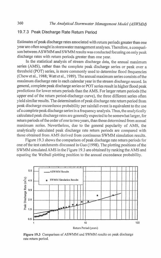
19.7.3 Peak Discharge Rate Return Period

Estimates of peak discharge rates associated with return periods greater than one year are often sought in storm water management analyses. Therefore, a compari-son hehveen ASWMM and SWMM results was t(xusing on onlY discharge rates with return periods greater than one year.

In the statistical analysis of stream discharge the fl.mmal ma.ximum series (AMS), rather than the complete peak discharge series or peak over a threshold (POT) series, is more commonly used to determine flood frequencies (ChO\v et at, i 988; 1989). The annual maximum series consists ofthe maximum discharge rate in each calendar year in the stream discharge record. In general, completl~ peak discharge series or POT series result in higher flood peak predictions for lower return periods than the AMS. For larger return periods (the upper end ofthe return period-discharge curve), the different series often yield similar results. The determination of peak discharge rate return period from peak discharge exceedance per rainfall event is equivalent to the use of a complete peak discharge series in a frequency analysis. Thus, the calculated peak discharge rates are generally expected to be somevvhat return periods ofthe order of one to two years, than those deterrnined from ammal maximum series. Nevertheless, to the genera! popularity of the analytically calculated discharge rate rerum periods are with those obtained from AMS derived from continuous S\Vl'vThll simUlation results,

Figure 19.3 shows the com.parison of peak rate return for one ofthe test catchments discussed in Guo (1998). The plotting positions ofthe SWMM simulated AMS in the Figure 19.3 are obtained mnkingthe AMS and equating the Weibull plotting position to the annual exceedance probability.

5.5. _ASWMM Resul,s

m SWMM Simul.tion Reslllts

10

Return Period (years)

Figure 19.3 Comparison of ASWlviM and SWMl'v1 results on peak discharge rate return period.

19.7 Verification of the ASWlvfM 361

The tc values required for input to the ASWMM are estimated using kinematic wave theory in accordance with a procedure outlined in Guo (1998). In practical applications, observed single event rainfall-runoff data may be used to estimate te' This estimated tc can then be used as input to ASWMM. The process of estimating tc for analytical models is equivalent to the calibration of numerical hydrological models by adjusting values of parameters such as slope, roughness and width of the catchment to match observed runoff hydro graphs.

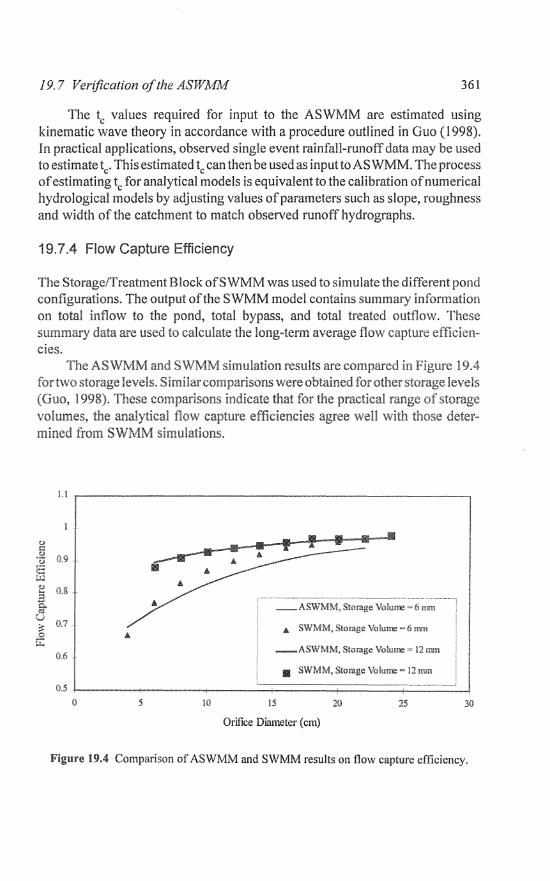
19.7.4 Flow Capture Efficiency

The Storage/Treatment Block ofSWMM was used to simulate the different pond configurations. The output of the SWr'llM model contains summary infol1nation on total inflow to the pond, total bypass, and total treated outflmv. These summary data are used to calculate the long-term average flow eftlden­des.

The ASWl'viM and SWMM simulation results arc compared in Figure 19.4 rort\vo storage levels. Similan:::omparisons were obtained levels (Guo, 1998), These indicate that fur the practical range volumes, the analytical capture efficiencies agree well \'lith those mined trom SWMM simulations.

u r:;; .~ t).9 C> .-ffi .., .... '" 0-N

V 0.7

~ ..9

... SWh1rvi, Stomge Voh.ure = 6 mal

::.:.. 116

_ASWMM, St;nagc Vol",n!! = 12ll'ml

lIIII SWMM, Slornge Vo!mre ~c 12 IT.n

0.5

(I 5 15 25 30

Orifice Diameter (cm)

l"igllre 19,4 Comparison of ASWMM and SWMM results on flow capture efficiency.

362 The Analytical Storm water Management Model (.4SWMA1)

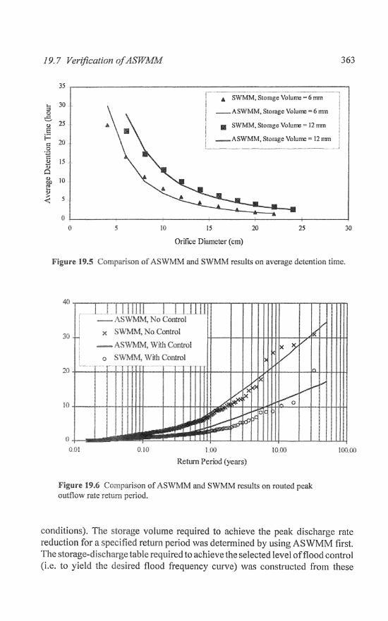
19.7.5 Average Detention Time

SWMM does not explicitly output detention times for individual runoff events routed through a pond, nor does it output average detention time ofa pond in long­term continuous simulation mode. Ho\vever, the inflow and outflow series from a long-term continuous simulation can both be separated into discrete events based on a minimum intcrevent time definition and a minimum threshold flow value. The time bases of the individual inflow and outflow events can subse­quently be determined. For an individual runoff event, the volume-weighted detention time is the distance between the centroids ofihe inflow and outi1mv hydrographs, which can be approximated by half of the difference between the time bases of the outflow and inflow hydro graphs. In cases where the pond is not empty when a new event starts, the time base of the outflow hydrograph terminates at the time the new event begins.

Obviously, the volume-weighted detention time for individual events calculated using the above procedure from SWMM siirmlation results will vary from event to event. Hmvever, an average volume-\veighted detention per runoff event can be estimated by averaging the detention times of ail the events within the simulation period. This average volume-vieighted detention time can be determined by calculating the total durations ofthe inflow and outflow' eYents. The total duration of outflow events from the pond, and the total duration of inflow events to the pond are the sums ofthe time bases ofthe outflow and inflmv events, respectively. The average detention time per event can then he calculated as hal f ofthe di ffcrence between the total outflow and inf10w durations divided by the total nmnber of inflow runoff events. in distinguishing runoff events, an IETD was used for the inflow series, since a 6 hr. IETD was used for separating rainfall events. The IETD for the outflow series is less critical since it does not affectthe total duration of outflow events. A minimum threshold flow value of 10-5 m3/s was used for both the inflow and outflow series.

Comparisons of ASWMM and SWMM results on average detention time for two sets of pond configurations are presented in Figure 19.5. More compari­sons can be found in Guo (1998). As shown in figure 19.5, the analytical results are in close agreement with those determined from SWMM simulations for the ranges of storage volumes and detention times analyzed.

19.7.6 Peak Outflow Rate Return Period

The comparison between the return period curves of peak outflow (from a Hood control detention pond servicing an urban catchment) detenninecl from ASWMM and from continuous SWMM is presented in Figure 19.6. For this comparison. a desired flood frequency curve was first chosen by selecting discharge rate values for each return period (Le. 50% reduction from those under ul1<.:ontro!led

19.7 Verification (jfASW.A,£lt,1

35

:.. 30

'" 0 e 25 <J

E [.::

20 e! 0 0g

15 B <> c <Jj !O Ol) ro .-'" ;:.-

5 -:(

5 10 15

do SWMM, Stornge Volume '" 6 rom

__ AS\VMM) Storage VoluOE=6mm

IIIIi SWMM, Storage Vohm-.: = 12 rnm

~~ASWMM. Storage Volume = 12 mm

20 25

Orifice Dinmeter (em)

363

30

Figure 19.5 'n~'n~.ic<", of ASWMivl and SWMM results on average detention time.

Return Period (years)

'o'"m''''l~(''' of ASWlvfM and SWMM results on routed peak outflow mte return period.

conditions). The storage volume required to achieve the peak discharge rate reduction for a specified return period was determined by using ASWMM first. The storage-discharge table required to achieve the selected level of flood control (i.e. to yield the desired flood frequency curve) was constructed from these

364 The Analytical Storm water Management Model (ASWMPv1)

storage volumes and peak discharge rates in the order ofincreasing return period. The storage-discharge table constructed by using ASWMM was then used as input data for the corresponding SWMM model.

In Figure 19.6, the analytical flood frequency curve and data points from simulation results when there is no flood control in place for the test catchment are also included. It is shown in Figure 19.6 thatthe ASWMM curves agree quite well with SWMM simulation results. More comparisons are presented in Guo (1998). These comparisons demonstrate that AS\VMM reasonably approximates the continuous simulation results on the flood control perfonnance of detention facilities.

19.8 Application of ASWMM

Except for Equations 19.3 and 19.8, the other ASWMM expressions which are not included in this chapter are lengthy and not suitable for hand calculations. instead, the analytical expressions can be easily coded into a computer spread­sheet. Given that statistical analysis of long-term historical rainfall data is perfol1ned a priori, with such a spreadsheet, the runoff event volume return period, peak discharge rate return period, and the performance of stormwater quality and flood control detention ponds can be evaluated with relative ease. For planning and design purposes, it is convenient to directly solve for runoff event volume or peak discharge rate with a specified return period, as well as the storage volume required to achieve a specified performance level. However, most ofthe analytical expressions are transcendental equations and some of them cannot be reduced to algebraic equations. Explicit analytical expressions for the peak discharge rate of a certain return period or the required storage volume for achieving certain level of perfonnancc cannot be derived. But these unknowns can be efficiently detennined in a computer spreadsheet by trial-and-eITor.

Figure 19.7 is a sample spreadsheet for the application of ASWMM for flood control analyses. The upper half of the spreadsheet is for the input of meteorological and hydrological parameters, while the lower half is for calcula­tion and plotting of the results. The meteorological parameter values for a given location are detennined a priori by statistical analysis of the long-tenn rainfall record of the location. In the lower half of the spreadsheet, the first two columns are simply the storage-discharge table of the detention facility. The third column is the return period of the peak discharge rate equaling the discharge rate ofthe detention facility with the installation ofthe flood control detention facility. The third column is thus a formula column incorporating the corresponding ASWMM expressions. The graph to the right of the three columns is the plot of Column 2 versus Column 3.

19.8 Application ofASW.M.J\-f

Hood Control Detention Facility Sizing Procedure

Local Meteorologll:aJ Parameters

A {}

O.W6J 0.1294 57.2

l/mm Vh events

(The inverse of the mean rainfall event volume.) (The inverse ofthe mean rainfall event duration.) (The average number of rainfall events pef year.)

Uscr Input Parameters Catchment Area, A =

Catchment Hydrological P!u"ameters

Fraction ofImpervious Areas, h =

Impervious Area Depression Storage, S <Ii =

Pervious Area Depression Storage.

Pervious Area Ultimate infiltration Capacity,fc =

Perviolls Area fuililll Soil Wetting Infiltration, S i .. =

Catchment Time of CO!1Ci;lltration, t c =

Calculated Pammeiers

PerviolL''i Area Initial Loss(;,~,

=hSdi + (l-h)S,!= TIll.: Dificrence Betwe,,;u Pervious and Impervious Area initial 1..05:;'::s, ------~~".".-".-... ------.--------

-- -(W-·-

1 460(J :UG6 l.O 27600 5.078 5.0 33190 6.383 lOJJ 40640 gl82 25.0 46330 9.587 50.0

200 hectares

0.35 1.5 mm

4.5 mm

3.6 mmlh

13.2 mm 2.1 hours

17.7 mm

12.03 mOl

16.2 mm

Return Period (years)

Figure 19:7 Sample spreadsheet implementation of ASWMM.

365

The above can be used to determine the flood control effective-ness of a given design. This is performed by simply inputting the storage­discharge relationship ofthe detention facility into Columns 1 and 2 in the lower half of the spreadsheet, and the related catchment and meteorological data in the upper half ofthe spreadsheet. The return periods in Column 3 in the lower half of the spreadsheet are then automatically calculated, and the plot of peak

366 The Analytical Storm water Management Model (ASWMNf)

discharge rate versus return period is automatically generated. The results can be examined to determine if the intended flood control objective is satisfied.

In planning and design situations, the catchment hydrologic parameters are input to the upper half of the spreadsheet first If the design criterion is specified in the form of controlling peak discharges of a series of return periods at certain levels (as is usually the case for most jurisdictions throughout North America), the series of discharges of specified return periods are input to Column 2 first, the required storage volumes to yield the desired return periods are determined by trial-and-error in Column 1 (i.e. different storage volumes in Column 1 are tried until the desired return period in Column 3 is obtained).

19.9 Conclusions

The exponential pdfs of rainfall event characteristics, tested and accepted in previous research for various locations, are used in this research as the starting point for the derivation ofthe analytical expressions constituting AS WMM. The close agreement betvveen ASWMM and SWMM results indicates that the event­based rainfall-nmofftransformation generates runoffvoiumes comparable with those from time-step based rainfaH-runofftransfonnations used in many numeri­cal hydrologic models. Furthermore, the close agreement of results illustrates that the exponential distributions used for rainfall event characteristics and the assumptions invoked for the simplification ofille mathematical representation of catchment runoff routing and detention pond flow routing are acceptable in practice.

Implemented in computer spreadsheets, ASVv'IvtM can be used very effi­ciently for the determination of the probability distribution of runoff event volume and peak discharge rate from urban catchments, as well as for the determination of the performance of stormwater quality and flood control detention ponds servicing urban catchments. More complete discussions of the development, implementation, and limitations of ASWMM can be found in Guo (1998).

Notation

a slope of the storage-discharge curve of a detention pond, h. b interevent time, h. b the mean interevent time of a long-term rainfall record, h. CR flow capture efficiency. E(·) expected value of (').

Notation

p

Ie

fB(b) fret) fv(v) h M N p

PP Pc Pc q Qj

t

t

v

e

ultimate infiltration capacity of a soil, mm/h. probability density function of random variable h. probability density function of random variable 1. probability density function of random variable v. fraction of impervious areas of an urban catchment rank of an event in a descending series of events. total number of rainfall events in a given period. total spill volume, mm. plotting position. carryover spin volume, mm. event spill volume, mm. a given peak discharge rate, mmlh or m3/5.

367

inflow rate to a flood control detention facility resulting from a runoff event, mmlh. peak outflow rate n'om a flood control detention facility result ing from a runoff event, mm/h.

discharge rate of a runoff event, mmlh or m3/s. area-weighted average depression storage of a catchment, mm. depression storage of the impervious areas of an urban catch

mm. Ihe difference bet\veen the depression storage values of the pervious and impervious areas of an urban catchment, mm.

storage of the pervious areas of an urban catchment, mm. Initial losses of the pervious areas of an urban catchment, • J d' ~ d" mC,lJ mg Siw an Sdp' mm. initial soil wetting infiltration volume, mm. HHLximum possible infiltration loss volume during a rainfall

mm. et;",.,,,,,, volume utilized when a detention pond is discharging at a rate of Q, mm. rainfall event duration, h. the mean of rainfall event duration of all rainfall events con tain~d in a long-term rainfall record, h. catchment time of concentration, h. rainfall event voiume, mm. the mean of rainfall event volume of ail rainfall events con tained in a long-term rainfall record, mm. runoff event volume, mm. parameter in the probability density function for rainfall event duration t, h-1

average annual number of rainfall events.

368

References

The Analytical Storm water Management Model (ASWMft,f)

parameter in the probability density function for interevent time b, h-1

parameter in the probability density function for rainfall event volume v, mm- l

Adams, B. J., and J. B. Bonije,! 984. Microcomputer applications of analytic a! models for urban stormwater management, in Emerging Computer Techniques in Stormwater and Flood Management, W. James (ed,), ASCE, New York, N. Y., 138-162.

Adams, B. J., H. G. Fraser, C. D. D. Howard, and M. S. Hanafy, 1986. Meteorologic data analysis for drainage system design, Journal of Enviromental Engineering, ASCE, VoL 112, No.5, 827-848.

Adams, B. J., and C. D. D. Howard,1986. Design stonn pathology, Canadian \Vater Resources Journal, Vol. 11, No.3, 49-55, Canadian Vvater Resources Association.

Benjamin, J. R., and C. A. Cornell, 1970. Probability, Statistics and Decision for Civil Engineers, McGraw-Hill, NeVI York.

Chow, V. T., D. R. Maidment, and L. W. Mays, 1988. Applied Hydrology, McGraw-Hill Book Company, New York, Nev. York, 1988.

Eagleson, P. S., Dynamics offload frequency, 1972. \Vater Resources Research, Vol. 8, No.4, 878-897.

Fraser, H. G., 1982. Frequency ofStonn Characteristics: Analysis and implications for Volume Design, M.A.Sc. thesis, Department of Civil Engineering, University of Toronto, Toronto, Ontario.

Guo, Y., 1988. Development of Analytical Probabilistic Urban Stormwater Models, Ph.D. thesis, Department of Civil Engineering, University of Toronto, Toronto, Ontario.

Howard, C. D. D., 1976. Theory of storage and treatment plant overflows, Journal of Environmental Engineering, ASCE, VoL 102, No. EE4, 709-722.

Huber, W. C., and R. E. Dickinson, 1988. Stormwater Management lvlodeJ, Version 4: User's Manual, Environmental Research Laboratory, Office of Research and Devel­opment, U. S. Environmental Protection Agency, Athens, Georgia, August, 1988.

Marsalek, J., 1978. Research on the design storm concept, Tech. lI:lemo. 33, ASCE, Urban Water Resources Research Program, New York.

Restrepo-Posada, P. J., and P. S. Eagleson, 1982. Identification of independent rain­storms, Journal of Hydrology, VoL 55, 303-319.

Robinson, M. and W. James, 1984. Continuous variable resolution storm water modelling on a microcomputer, Proceedings, Conference on Stoml'vvater and Water Quality Management Modeling, September 1984, Burlington, Ontario, E. M. and W. James (eds.), McMaster University, 59-73.

Walesh, S. G., 1989.Urban Surface Water Management, John Wiley & Sons, Inc., New York.

\Vatt, W. E., et a!. 1989. Hydrology of Floods in Canada: A Guide to Planning and Design, National Research Council of Canada, Ottawa, Ontario.

References 369

Wenzel, H. G" Jr., 1982. Rainfall for urban stormwater design, in Urban Stormwater Hydrology, Water Resources Monograph 7, D. F. Kibler (ed.), American Geophysical Union, Washington, D. C.

Wenzel, H. G., Jr., and M. L. Voorhees, 1978. Evaluation ofthe design storm concept, paper presented at the American Geophysical Union Annual Fall Meeting, San Francisco, California, December 1978.

Wenzel, H. G., Jr., and M. L. Voorhees, 1979. Sensitivity of design storm frequency, paper presented at the American Geophysical Union Annual Spring Meeting, Washington, D. C., May 1979.

I I I I I I I I I I I I I I I I I I I I I I I I I I I I I I I I I I I I I I I I I I I I I I I I I I I I I I I I I I I I I

I I I I I I I I I I I I I I I I I I I I I I I I I I I I I I I

I I I I I I I I I I I I I I I

I I I I I I I I

I I I I

I I

I I I I