The American frontier: Technology versus immigration - Guillaume

Review of Economic Dynamics 11 (2008) 283–301

www.elsevier.com/locate/red

The American frontier: Technology versus immigration ✩

Guillaume Vandenbroucke

Department of Economics, University of Southern California, 3620 S. Vermont Ave., KAP 324F, Los Angeles, CA 90089-0253, USA

Received 22 May 2006; revised 30 June 2007

Available online 11 August 2007

Abstract

How important was international immigration for the US and its demography during the nineteenth century? This paper inves-tigates, quantitatively, its effect on the westward movement of population and the regional and secular changes in fertility. Besideimmigration, two alternative forces are considered: technological progress and the land policy (the Homestead Act). An optimalgrowth model with endogenous fertility and migration is calibrated, and counterfactual experiments reveal that the main drivingforces were productivity growth and the declining cost of transportation. International immigration played a lesser role.© 2007 Elsevier Inc. All rights reserved.

JEL classification: E1; J1; O1

Keywords: Population growth; Migration; Fertility; Technological progress; US westward expansion

1. Introduction

The United States is often viewed as a “country of immigrants.” The fact is that, during the nineteenth century,the rate of international immigration averaged five percent per decade, accounting from seven percent of the rate ofpopulation growth during the 1820s to 33% during the 1850s.1 Panel A of Fig. 1 shows the decomposition of thegrowth rate of population, and the contributions of the rates of net migration and natural increase. Panel B proposesa simple exercise to assess the importance of international immigration. It shows the US population vis à vis thepath that would have occurred if population grew at its rate of natural increase. The result is remarkable: withoutinternational immigration, the US population in 1900 would have been 52% below its actual value. This exercisesuggests that immigration mattered, but it assumes that the rate of natural increase was no affected by immigrants.This paper proposes to relax this assumption and to use the optimal growth model to study the key patterns of the USdemography during the nineteenth century. The objective is to measure the impact of immigration versus alternativedriving forces, such as various aspects of technological progress, and the land policy set by the US government—thatis the mechanism through which the government attempted to regulate the settlement of the western territories.

✩ This is a revised version of the third chapter of my dissertation submitted to the University of Rochester, and previously circulated under thetitle “The American Frontier: One Hundred Years of Western Settlement.”

E-mail address: [email protected] See Haines (2000, Table 4.1).

1094-2025/$ – see front matter © 2007 Elsevier Inc. All rights reserved.doi:10.1016/j.red.2007.07.001

284 G. Vandenbroucke / Review of Economic Dynamics 11 (2008) 283–301

(A) (B)

The source of data is Haines (2000, Table 4.1). Panel A represents the growth rate of total population, per decade, and its decomposition betweennatural increase and net migration. This decomposition is based on the following accounting equation, where pt represents total population:

pt+1 − pt

pt= #birthst − #deathst

pt+ #immigrantst − #outmigrantst

pt.

The first element on the right-hand side is the rate of natural increase and the second element is the rate of net migration. Panel B represents thelevel of population, normalized to one in 1800, and the path that the rate of natural increase alone would have implied.

Fig. 1. Population Growth in the United States, 1800–1900.

The paper proceeds as follows. The rest of this section presents the main facts of interest and discusses potentialexplanations. In particular, Section 1.1 documents the trends in regional fertility and the geographic distribution ofpopulation. Section 1.2 hypothesizes that technological progress, in various activities, can be an alternative to inter-national immigration in generating these trends. Section 2 presents the model and Section 3 the quantitative analysis.The latter consists first in matching the model to the US data and, then, running a set of counterfactual experimentsto assess the quantitative importance of each exogenous force built into the model. The conclusion of this exercise isthat immigration had a “smaller-than-expected” impact on the US demography, while transportation costs and wagegrowth mattered significantly. Specifically, one experiment shows that international immigration directly affected therate of population growth, but hardly affected the rate of natural increase and the geographic distribution of population.Another experiment shows that technological progress in transportation and in the production of goods drove most ofthe geographic distribution of population. Finally, the paper considers two land policies. The baseline policy is remi-niscent of the Homestead Act, i.e., when the US government gave the land out to those who settled it without titles.The alternative policy is reminiscent of the auction mechanism often used to sell acres of western land to the public.Interestingly, the two policies led to very similar results in terms of western settlement. However, they affected the rateof natural increase differently: under the Homestead Act, population growth was slower than when the governmentsold the land. Section 4 presents some concluding remarks.

1.1. Facts

What were the key patterns of the US demography during the nineteenth century? First, there was internationalimmigration as mentioned above. It is interesting to know that immigrants settled in all regions of the country. AsTable 1 shows, the proportion of foreigners rose both in the East and the West between 1820 and 1860.

In addition to high rates of net migration, the US demography was also characterized by high rates of naturalincrease compared with the rest of the world. At a more disaggregated level, there were sharp regional differences.In particular, the rate of population growth in the West was higher than in the East, as illustrated by the changinggeographic distribution of population in Fig. 2—the source of data is Mitchell (1998, Table A.3). This phenomenon,often referred to as the “Westward Expansion,” shaped the US as we know it today. By the end of the nineteenthcentury the rates of population growth in each region have converged, and the geographic distribution of populationbecame stationary.

G. Vandenbroucke / Review of Economic Dynamics 11 (2008) 283–301 285

Table 1Percent of Foreign Born per Region, 1820 and 1860

1820 1860 1820 1860

New England Middle AtlanticMaine 0.57 6.00 New York 1.13 26.10New Hampshire 0.05 6.40 New Jersey 0.59 19.00Vermont 0.40 10.40 Pennsylvania 1.05 15.10Massachusetts 0.66 22.20Rhode Island 0.30 21.90Connecticut 0.21 17.90East North Central West North CentralOhio 0.61 14.20 Minnesota – 34.70Indiana 0.57 8.80 Iowa – 15.70Illinois 1.11 19.00 Missouri 0.89 15.10Michigan 7.63 20.30 Dakota – 68.90Wisconsin – 35.80 Nebraska – 22.10

Kansas – 11.90

The source of data is Yasuba (1962, Table V-17).

The “East” is arbitrarily defined as the New-England, Middle-Atlantic and South Atlantic regions. The list of states in these regions are Maine, NewHampshire, Vermont, Massachusetts, Rhode Island, Connecticut, New York, New Jersey, Pennsylvania, Delaware, Maryland, District of Columbia,Virginia, West Virginia, North Carolina, South Carolina, Georgia and Florida. The West consists of all other states in the continental US.

Fig. 2. Regional shares of total population, US, 1790–1910.

The faster population growth experienced by the West was due, at the same time, to high rates of net migration andnatural increase relative to the East. To illustrate the importance of western migration, consider the East North Centralstates: Ohio, Indiana, Illinois, Michigan and Wisconsin.2 During the early stages of the century this region was thewestern Frontier of the country, and Fig. 3 shows the decomposition of the growth rate of its population—the sourceof data is Gallaway and Vedder (1975, Table 1). Net migration accounted for more than 80% of population growth

2 Similar data are not available for the entire century because the US census did not systematically collect data on population by state of birthand state of residence before 1850.


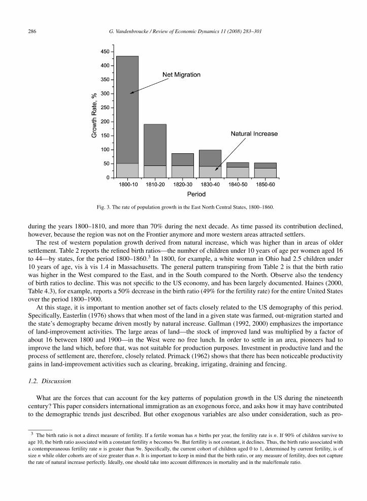
Fig. 3. The rate of population growth in the East North Central States, 1800–1860.

during the years 1800–1810, and more than 70% during the next decade. As time passed its contribution declined,however, because the region was not on the Frontier anymore and more western areas attracted settlers.

The rest of western population growth derived from natural increase, which was higher than in areas of oldersettlement. Table 2 reports the refined birth ratios—the number of children under 10 years of age per women aged 16to 44—by states, for the period 1800–1860.3 In 1800, for example, a white woman in Ohio had 2.5 children under10 years of age, vis à vis 1.4 in Massachusetts. The general pattern transpiring from Table 2 is that the birth ratiowas higher in the West compared to the East, and in the South compared to the North. Observe also the tendencyof birth ratios to decline. This was not specific to the US economy, and has been largely documented. Haines (2000,Table 4.3), for example, reports a 50% decrease in the birth ratio (49% for the fertility rate) for the entire United Statesover the period 1800–1900.

At this stage, it is important to mention another set of facts closely related to the US demography of this period.Specifically, Easterlin (1976) shows that when most of the land in a given state was farmed, out-migration started andthe state’s demography became driven mostly by natural increase. Gallman (1992, 2000) emphasizes the importanceof land-improvement activities. The large areas of land—the stock of improved land was multiplied by a factor ofabout 16 between 1800 and 1900—in the West were no free lunch. In order to settle in an area, pioneers had toimprove the land which, before that, was not suitable for production purposes. Investment in productive land and theprocess of settlement are, therefore, closely related. Primack (1962) shows that there has been noticeable productivitygains in land-improvement activities such as clearing, breaking, irrigating, draining and fencing.

1.2. Discussion

What are the forces that can account for the key patterns of population growth in the US during the nineteenthcentury? This paper considers international immigration as an exogenous force, and asks how it may have contributedto the demographic trends just described. But other exogenous variables are also under consideration, such as pro-

3 The birth ratio is not a direct measure of fertility. If a fertile woman has n births per year, the fertility rate is n. If 90% of children survive toage 10, the birth ratio associated with a constant fertility n becomes 9n. But fertility is not constant, it declines. Thus, the birth ratio associated witha contemporaneous fertility rate n is greater than 9n. Specifically, the current cohort of children aged 0 to 1, determined by current fertility, is ofsize n while older cohorts are of size greater than n. It is important to keep in mind that the birth ratio, or any measure of fertility, does not capturethe rate of natural increase perfectly. Ideally, one should take into account differences in mortality and in the male/female ratio.


Table 2Number of children under 10 years of age per 1000 women aged 16–44, US, 1800–1860

1800 1810 1820 1830 1840 1850 1860

New EnglandMaine 1974 1883 1621 1463 1416 1217 1108New Hampshire 1704 1558 1385 1207 1112 915 900Vermont 2068 1788 1468 1341 1286 1131 1079Massachusetts 1477 1421 1269 1064 987 857 895Rhode Island 1455 1405 1314 1139 989 910 887Connecticut 1512 1438 1280 1114 1040 915 930

Middle AtlanticNew York 1871 1895 1706 1466 1273 1070 1063New Jersey 1822 1736 1629 1457 1360 1208 1150Pennsylvania 1881 1841 1748 1536 1456 1322 1293

South AtlanticDelaware 1509 1687 1596 1393 1332 1314 1269Maryland 1585 1598 1509 1302 1284 1237 1207Virginia 1954 1777 1710 1587 1544 1421 1408North Carolina 1920 1857 1822 1645 1606 1389 1351South Carolina 2030 1951 1851 1681 1635 1357 1324Georgia 2116 2103 2002 1962 1966 1672 1508Florida 1899 1705 1726 1568

East North CentralOhio 2550 2303 2131 1871 1696 1466 1360Indiana 2014 2307 2235 2139 1835 1702 1531Illinois 2201 2235 2175 1869 1607 1471Michigan 2121 1826 1834 1602 1463 1301Wisconsin 1569 1493 1594

East South CentralKentucky 2371 2271 2070 1891 1890 1597 1517Tennessee 2424 2302 2204 2033 1916 1594 1483Alabama 2252 2198 2075 1637 1536Mississippi 2509 2089 2222 2113 2053 1776 1582

West North CentralMinnesota 1508 1619Iowa 1837 1726 1636Missouri 2375 2189 2223 1960 1581 1532Dakota 1157Nebraska 1460Kansas 1496

West South CentralArkansas 2159 2205 2160 1843 1727Louisiana 1904 1845 1738 1597 1294 1320Texas 1745 1761

MountainColorado 764New Mexico 1265 1406Utah 1513 2004Nevada 1270

PacificWashington 1847Oregon 2005 2104California 1111 1287

The source of data is Yasuba (1962, Table II-7).

ductivity and/or transportation costs in various sectors. These technological factors are alternatives to the hypothesisthat international immigration alone was the cause of the demographic changes. Let us review, below, the argumentssuggesting that all these variables are sound driving forces.


To discuss the possible effects of international immigration, it is interesting to start by observing that the vastmajority of investment in productive land, after 1800, was done in the West. In other words, one can view the Easternseaboard of the US has having a fixed stock of productive land as off 1800, while in the West households couldaccumulate productive land. In an economy mostly dominated by agriculture, a fixed stock of land means decreasingreturns to scale. Thus, as total population grew, the West was the region where growth could be higher than in the East.In short, population growth may have “pushed” Americans out of the East toward the West. The question is: whichpart of population growth was the most important for this mechanism? The part driven by natural increase or the partdriven by international immigration?

How could technological progress have affected the US demography? First, and as mentioned earlier, there wasproductivity gains in land-improvement activities. These gains made the cost of settling into the West lower andcontributed to the westward migration. Second, technological progress also improved transportation for goods andpeople. This, again, contributed positively to the westward migration. Third, technological progress also permittedreal wage growth in the East despite decreasing returns to scale. This effect weakened the incentive to move westward.Finally, real wage growth affected the rate of natural increase through childbearing decisions. This point is discussedin more details below.

Birth ratios were higher in the West than in the East but they declined in both regions. By 1900, they had convergedto a common value.4 Various mechanisms could be responsible for the declining birth ratios. Greenwood et al. (2005),for example, suggest that raising children is a time-consuming activity so that, as the wage rate grows, the optimalnumber of children declines. This framework, however, predicts low fertility in high-wage regions, a contradictionto historical facts since the real wage rate was higher in the West than in the East.5 One can imagine, however, thatland availability in the West promoted higher fertility despite the opportunity cost of raising children. Yasuba (1962)suggests that in a rural economy, young individuals can establish themselves as households more easily if land ischeap. This promotes early marriage, and higher marital fertility than in areas where land is relatively less abundant.Another effect might come from the fact that a large family is a more valuable asset in rural areas than in urban areas:child labor can more easily be used on the family farm. Easterlin (1976) proposes a “bequest model” to rationalizethis. His model prescribes that parents feel concerned with the welfare of their offspring and decide how much to givethem for their start in life. In a land-abundant region it is cheaper to give one’s child a start in life than in a regionwhere land is less abundant. The first reason is that land is cheaper so endowing a child with a parcel of land is moreaffordable than elsewhere. Second, bequests do not have to be parcels of land. Parents may wish to endow their kidswith any form of non-physical capital. This was more easily achieved in a high-real-wage area like the West.

The link between fertility and land availability is quite solid. Yasuba (1962) reports rank correlations between thebirth ratio and a measure of land availability: the number of persons per 1000 acres of arable land. As he pointsout, one could argue that this measure also captures the urbanization movement that took place during the nineteenthcentury.6 To address this issue, he also computes the rank correlation between the birth ratio and the proportion ofurban population by states. Table 3 reports his results. From these numbers, he concludes that the relationship betweenfertility and density is “more than an indirect analysis of the relationship between urbanization and fertility.”

Table 3Rank correlations with the birth ratio, US, 1800–1860

1800 1810 1820 1830 1840 1850 1860

pop./acres of land −0.633 −0.848 −0.802 −0.773 −0.675 −0.604 −0.526prop. of urban pop. −0.468 −0.360 −0.544 −0.409 −0.495 −0.593 −0.366

The source of data is Yasuba (1962, Tables V.4 and V.10). The figures correspond to the rank correlation between the birth ratio and the populationper acres of land (or the proportion of urban population) across states.

4 See Easterlin (1976).5 See Coelho and Shepherd (1976) and Margo (2000).6 See Greenwood and Seshadri (2002) for an analysis of the relationship between urbanization and fertility.


2. The model

The economy has three noticeable features: fertility, migration and investment in land. A household lives for threeperiods: one as a child and two as an adult. Only young adults work. There are two locations called East and West, anda single consumption good is produced in each location with the services of labor, improved land and an intermediategood. The latter is produced in the East only, and there is a transportation cost associated with its use in the West.Another transportation cost is associated with labor moving from one location to the other.

The amount of land services in the East is fixed. In the West, there is a land-improvement sector that buys rawland from a government. It also hires western labor to operate its technology and sells newly improved land to thehouseholds who, in turn, rent it to the consumption-good sectors.

Preferences are defined over consumption and the number of children. Households can choose where to live, andthey make this choice only once in their life, at the beginning of adulthood, before deciding how many children tohave. The childbearing period is the first period of adulthood.

2.1. Firms

2.1.1. Intermediate goodThe technology is xt = zxth

ext where xt is the total output of the sector, zxt is an exogenous productivity parameter

and hext is eastern labor. Let qxt denote the price of x in the East. In the West, the price of the good is qxt (1 + τxt ),

where τxt is an iceberg cost representing the state of the transportation technology. The optimization problem of thefirm is:

maxhe

xt

{qxtxt − we

t hext

}, (1)

where wet denotes the eastern real wage rate.

2.1.2. Consumption goodThe technology in this sector is described by

yjt = zyt

(h

jyt

)μ(x

jt

)φ(ljt

)1−φ−μ, μ, φ ∈ (0,1),

where the superscript j refers to the location. The variables hjyt , x

jt and l

jt , are inputs of labor, intermediate good and

improved land, respectively. The objective of the eastern and western sectors are

maxhe

yt ,xet ,let

{yet − we

t heyt − qxtx

et − re

t let}

(2)

and

maxhw

yt ,xwt ,lwt

{ywt − ww

t hwyt − qxt (1 + τxt )x

wt − rw

t lwt}, (3)

where rjt denotes the rental price of improved land in location j .

2.1.3. Land-improvementEastern land is fixed: let = le. In the West, the variable lwt , which represents the productive services of improved

land, can increase. Specifically, the total stock of western land is fixed and represented by the unit interval, but thefraction of it which is improved and productive is a choice variable. The services of productive land, measured inefficiency units, are given by lwt = ∫ lt

0 Λ(u)du where lt is the stock of improved land measured in physical units, andΛ is the density of efficiency units of land. The density function is Λ(u) = 1 − uθ where θ > 0.

The technology for accumulating new productive land requires the use of labor only. Thus, the law of motion forthe stock of improved land is

lt+1 = lt + zlthwlt

where zlt is a technology parameter and hwlt is western labor employed in the sector. Observe that the stock of improved

land does not depreciate.


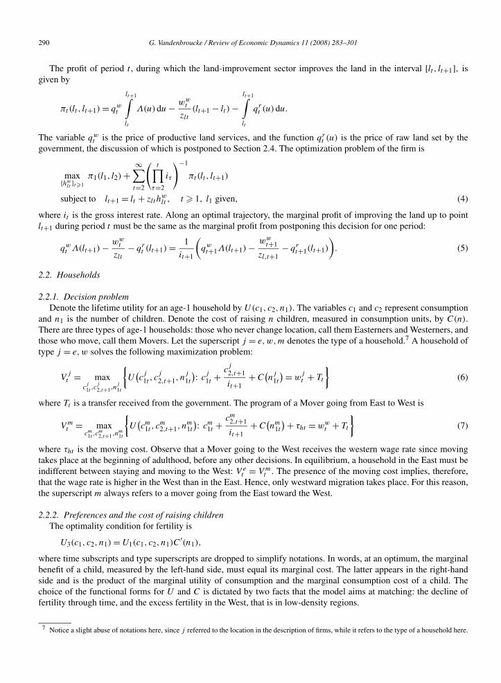
The profit of period t , during which the land-improvement sector improves the land in the interval [lt , lt+1], isgiven by

πt (lt , lt+1) = qwt

lt+1∫lt

Λ(u)du − wwt

zlt

(lt+1 − lt ) −lt+1∫lt

qrt (u)du.

The variable qwt is the price of productive land services, and the function qr

t (u) is the price of raw land set by thegovernment, the discussion of which is postponed to Section 2.4. The optimization problem of the firm is

max{hw

lt }t�1

π1(l1, l2) +∞∑t=2

(t∏

τ=2

iτ

)−1

πt (lt , lt+1)

subject to lt+1 = lt + zlthwlt , t � 1, l1 given, (4)

where it is the gross interest rate. Along an optimal trajectory, the marginal profit of improving the land up to pointlt+1 during period t must be the same as the marginal profit from postponing this decision for one period:

qwt Λ(lt+1) − ww

t

zlt

− qrt (lt+1) = 1

it+1

(qwt+1Λ(lt+1) − ww

t+1

zl,t+1− qr

t+1(lt+1)

). (5)

2.2. Households

2.2.1. Decision problemDenote the lifetime utility for an age-1 household by U(c1, c2, n1). The variables c1 and c2 represent consumption

and n1 is the number of children. Denote the cost of raising n children, measured in consumption units, by C(n).There are three types of age-1 households: those who never change location, call them Easterners and Westerners, andthose who move, call them Movers. Let the superscript j = e,w,m denotes the type of a household.7 A household oftype j = e,w solves the following maximization problem:

Vjt = max

cj1t ,c

j2,t+1,n

j1t

{U

(cj

1t , cj

2,t+1, nj

1t

): c

j

1t + cj

2,t+1

it+1+ C

(n

j

1t

) = wjt + Tt

}(6)

where Tt is a transfer received from the government. The program of a Mover going from East to West is

V mt = max

cm1t ,c

m2,t+1,n

m1t

{U

(cm

1t , cm2,t+1, n

m1t

): cm

1t + cm2,t+1

it+1+ C

(nm

1t

) + τht = wwt + Tt

}(7)

where τht is the moving cost. Observe that a Mover going to the West receives the western wage rate since movingtakes place at the beginning of adulthood, before any other decisions. In equilibrium, a household in the East must beindifferent between staying and moving to the West: V e

t = V mt . The presence of the moving cost implies, therefore,

that the wage rate is higher in the West than in the East. Hence, only westward migration takes place. For this reason,the superscript m always refers to a mover going from the East toward the West.

2.2.2. Preferences and the cost of raising childrenThe optimality condition for fertility is

U3(c1, c2, n1) = U1(c1, c2, n1)C′(n1),

where time subscripts and type superscripts are dropped to simplify notations. In words, at an optimum, the marginalbenefit of a child, measured by the left-hand side, must equal its marginal cost. The latter appears in the right-handside and is the product of the marginal utility of consumption and the marginal consumption cost of a child. Thechoice of the functional forms for U and C is dictated by two facts that the model aims at matching: the decline offertility through time, and the excess fertility in the West, that is in low-density regions.

7 Notice a slight abuse of notations here, since j referred to the location in the description of firms, while it refers to the type of a household here.


As mentioned earlier, the decline in fertility can be accounted for along the lines of Greenwood et al. (2005). Theirapproach suggests the following choices for preferences and the cost of raising children:

U(c1, c2, n1) = ln(c1 + c̄) + β ln(c2 + c̄) + σ ln(n1) (8)

and

C(n) = wn1

zk

, (9)

where σ > 0 and β ∈ (0,1). In this formulation, the parameter c̄ is a positive constant affecting the marginal utilityof consumption. Its purpose is to allow the analysis to benefit from the simplicity of the logarithmic utility, whileoffering flexibility in the choice of the curvature of the utility function. As will become transparent soon, this device isuseful to generate the decline in fertility. The parameter zk is a positive constant which measures the “productivity” ofnon-market time in the child-raising activity. The quantity n1/zk , therefore, is the time spent raising n1 children. Theconsumption cost of n1 children is the market value of this time. With these functional forms, the optimality conditionfor fertility writes

σ

n1= w/zk

c1 + c̄.

Observe that, along an equilibrium path where consumption and wages grow at the same rate the marginal cost ofa child increases and, therefore, fertility must decrease. Notice also that, when c̄ = 0, fertility is constant along abalanced growth path. Asymptotically, the effect of c̄ vanishes and fertility converges to this constant.

The framework above implies that fertility is lower in the West, where wages are higher. To solve this problem,the discussion in Section 1.2 suggested that the density of population could enter the first order condition for fertility.There are two approaches here. The first relies on a modification of preferences, the second on a modification of thechild-raising technology. As will become clear shortly, the two approaches share some similarities—a standard featureof household production models, pointed out by Benhabib et al. (1991).

The first approach consists in introducing density into the utility function. More precisely, let preferences be rep-resented by

U(c1, c2, n1) = ln(c1 + c̄) + β ln(c2 + c̄) + σ(

1 + κ

d

)ln(n1) (10)

where κ > 0 and d is the density of population in the region where the household is living. In a densely populated area,the marginal utility of a child is lower: a “crowding” effect. One can imagine, for example, that parents internalize thefact that a child born in a crowded area may have a harder time finding land and setting up his own farm. They deriveless utility from the child because they foresee that. The utility function in (10) proposes a shortcut to model this idea.The optimality condition for fertility, derived from combining (9) with (10), is(

1 + κ

d

) σ

n1= w/zk

c1 + c̄. (11)

With this framework, a higher wage rate does not necessarily imply lower fertility if the density is small enough. Aspopulation grows, all the land gets eventually improved and the density of population increases in each region. Thisimplies that in the long run the term κ/d converges to zero. Then, fertility choices converge if wages are convergingtoo.

Another approach to introducing density into the optimal fertility decision does not rely on preferences. It consistsin introducing the density into the cost of raising kids. One can imagine that, in low-density regions, it is easier tohave children working on a small area of land and contributing to the household’s income. Thus, although it still takestime to raise a child, this time cost is partly offset by “child labor.” Suppose, for example, that the time needed toraise one child is given by (1 + κ/d)−1/zk , which implies that the time cost of a child is increasing with density. Theconsumption cost for n1 children becomes

C(n1) = wn1

zk

(1 + κ

d

)−1. (12)

With this formulation, a high-wage low-density area can potentially have high fertility. When the land gets moresettled, it becomes harder to find such areas of land for children to work (e.g., the yard on the farm becomes smaller),


and the effect of density on the cost of raising children vanishes. The optimality condition for fertility, derived fromcombining (12) with (8), is again given by Eq. (11). In what follows, the cost function (9) and the utility function (10)are used.8

2.3. Demography

Let pwt and pe

t denote the number of age-1 Westerners and Easterners, respectively. Let pmt denote the number of

age-1 Movers going from East to West at date t . Movers are born in the East but leave it for the West. Their childrenare born in the West. Thus, the total age-1 western population is pw

t + pmt , while the total age-1 eastern population

is pet . Let f denote the rate of international immigration, and assume that immigrants arrive during the first period of

their life, and become age-1 adults during the next period. The law of motion for pwt is

pwt+1 = pw

t nw1t + pm

t nm1t + f

(pw

t + pmt

). (13)

This equation dictates that the number of age-1 Westerners at date t + 1 has three sources. First they can be born fromthe current generation of Westerners: pw

t nw1t . Second, they can be born from the current generation of Movers: pm

t nm1t .

Finally, they can also be moving into the West, directly from the rest of the world, in proportion f of the currentwestern population. The law of motion for pe

t is

pet+1 = pe

t ne1t − pm

t+1 + fpet , (14)

that is, age-1 Easterners at t + 1 are either born from the current generation or coming from the rest of the world. Theterm −pm

t+1 indicates that one has to subtract those who decide to move out of the East at date t + 1, since they arenot Easterners by definition. The total age-1 population evolves in line with

pwt+1 + pe

t+1 + pmt+1 = pw

t

(nw

1t + f) + pm

t

(nm

1t + f) + pe

t

(ne

1t + f).

The density of age-1 population in the East is det = pe

t / le and for the West it is given by dwt = (pw

t + pmt )/ lwt .

2.4. Land policy

During the nineteenth century the land policy changed a number of times, and was the subject of intense politicaldebates.9 The general rule was that western raw land was sold to settlers, by the US government, through an auctionprocess. The difficulties found in enforcing property rights on the frontier, however, forced the US government torecognize squatters and legalize their occupancy of the land at a number of occasions throughout the century. In 1862,the Homestead Act was passed which, essentially, consisted in giving the land out for free. Formally, the HomesteadAct writes qr

t (u) = 0 for all t and u. The consequence of this subsidy (giving out free land) is that the government hasno resources to transfer to households, hence Tt = 0. Later, the quantitative analysis section considers an alternativeland policy.

2.5. Equilibrium

2.5.1. Definition of equilibriumIn equilibrium bonds and land must deliver the same rate of return, hence

it+1 = rj

t+1 + qj

t+1

qjt

, j = e,w. (15)

The western and eastern labor markets must clear:

8 Notice that, although the two approaches deliver the same first order condition for fertility, they are not equivalent since they involve differentvalue functions and, therefore, different allocations. As will appear in Section 3.1, however, the methodology used in the empirical exercise impliesthat the quantitative difference between the allocations obtained with each method is small.

9 See Atack et al. (2000).


pwt

(1 − nw

1t /zk

) + pmt

(1 − nm

1t /zk

) = hwyt + hw

lt , (16)

pet

(1 − ne

1t /zk

) = heyt + he

xt . (17)

In Eqs. (16) and (17) the left-hand side are western and eastern labor supplies, taking into account the time spentraising children for each type of household. The right-hand side are labor demands from the sectors operating in eachregion. The market for the intermediate good must clear too:

xwt + xe

t = xt . (18)

Finally, the market clearing condition for savings is

pwt sw

t+1 + pmt sm

t+1 + pet s

et+1 = qw

t lwt+1 + qet l

e (19)

where sj

t+1 are the savings of an age-1 household of type j during period t , which will pay off during period t + 1.

Definition 1. A competitive equilibrium is composed of: (i) allocations for households {cjat , n

j

1t } for j = e,w,m and

a = 1,2 and firms {hwyt , h

wlt , h

eyt , h

ext , l

e, lwt }; (ii) prices {wjt , r

jt , q

jt , qxt , it } for j = e,w, such that

(1) The sequence {hext } solves (1) at all t given prices;

(2) The sequence {heyt , x

et , l

e} solves (2) at all t given prices;(3) The sequence {hw

yt , xwt , lwt } solves (3) at all t given prices;

(4) The sequence {hwlt } solves (4) given prices;

(5) The sequences {cjat , n

j

1t } for j = e,w solve (6) given prices; the sequence {cmat , n

m1t } solves (7); and households

choose their location optimally, that is V et = V m

t ;(6) Population growth is described by (13) and (14);(7) Market clears, or conditions (15)–(19) hold.

2.5.2. Balanced growthIn the long run all the land is improved in the West: lwt → ∫ 1

0 Λ(u)du ≡ lw, as t → ∞. Hence, employmentin the land-improvement sector converges to zero: hw

lt → 0. Assume that transportation costs converge to zero too:τht , τxt → 0 as t → ∞, implying that eastern and western wages converge. Let total factor productivity grow by afactor gz > 1 per period, in the consumption and intermediate good sectors, and assume that gz is large enough towarrant wage growth. In such case, fertility is the same for all types and is constant through time.10 Denote it by n1so that, in each location, the rate of population growth is n1 + f. Then, output in the intermediate good sector growsat rate gz(n1 + f ) and the growth rate of the economy becomes

g = g1+φz (n1 + f )φ+μ.

Real wages are growing at rate g/(n1 + f ). The optimality conditions for households imply that individual consump-tion and savings grow at the same rate as real wages. Thus aggregate consumption grows at rate g. Since the stock of

10 The first order conditions for problem (6) when the cost function (9) and the utility function (10) are used are

cj1t

+ c̄

wjt

= 1

1 + β

(1 − n

j1t

zk+ c̄

wjt

(1 + 1

it+1

))

and

cj1t

+ c̄

wjt

= nj1t

/zk

σ

(1 + κ

djt

)−1.

In the long run the terms c̄/wjt and κ/d

jt converge to zero so that

nj1t

zk

(1

σ+ 1

1 + β

)= 1

1 + β.

Hence, in the long run, fertility is constant and identical for Easterners, Westerners and Movers.


land is fixed, the price of land must grow at rate g too. The firms optimality conditions imply also that the rental ratefor land increases at rate g, hence Eq. (15) implies a constant interest rate.

3. Quantitative analysis

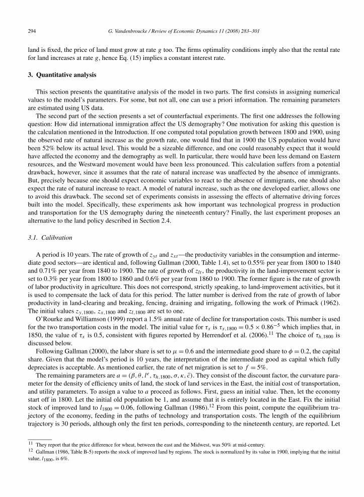
This section presents the quantitative analysis of the model in two parts. The first consists in assigning numericalvalues to the model’s parameters. For some, but not all, one can use a priori information. The remaining parametersare estimated using US data.

The second part of the section presents a set of counterfactual experiments. The first one addresses the followingquestion: How did international immigration affect the US demography? One motivation for asking this question isthe calculation mentioned in the Introduction. If one computed total population growth between 1800 and 1900, usingthe observed rate of natural increase as the growth rate, one would find that in 1900 the US population would havebeen 52% below its actual level. This would be a sizeable difference, and one could reasonably expect that it wouldhave affected the economy and the demography as well. In particular, there would have been less demand on Easternresources, and the Westward movement would have been less pronounced. This calculation suffers from a potentialdrawback, however, since it assumes that the rate of natural increase was unaffected by the absence of immigrants.But, precisely because one should expect economic variables to react to the absence of immigrants, one should alsoexpect the rate of natural increase to react. A model of natural increase, such as the one developed earlier, allows oneto avoid this drawback. The second set of experiments consists in assessing the effects of alternative driving forcesbuilt into the model. Specifically, these experiments ask how important was technological progress in productionand transportation for the US demography during the nineteenth century? Finally, the last experiment proposes analternative to the land policy described in Section 2.4.

3.1. Calibration

A period is 10 years. The rate of growth of zyt and zxt —the productivity variables in the consumption and interme-diate good sectors—are identical and, following Gallman (2000, Table 1.4), set to 0.55% per year from 1800 to 1840and 0.71% per year from 1840 to 1900. The rate of growth of zlt , the productivity in the land-improvement sector isset to 0.3% per year from 1800 to 1860 and 0.6% per year from 1860 to 1900. The former figure is the rate of growthof labor productivity in agriculture. This does not correspond, strictly speaking, to land-improvement activities, but itis used to compensate the lack of data for this period. The latter number is derived from the rate of growth of laborproductivity in land-clearing and breaking, fencing, draining and irrigating, following the work of Primack (1962).The initial values zy,1800, zx,1800 and zl,1800 are set to one.

O’Rourke and Williamson (1999) report a 1.5% annual rate of decline for transportation costs. This number is usedfor the two transportation costs in the model. The initial value for τx is τx,1800 = 0.5 × 0.86−5 which implies that, in1850, the value of τx is 0.5, consistent with figures reported by Herrendorf et al. (2006).11 The choice of τh,1800 isdiscussed below.

Following Gallman (2000), the labor share is set to μ = 0.6 and the intermediate good share to φ = 0.2, the capitalshare. Given that the model’s period is 10 years, the interpretation of the intermediate good as capital which fullydepreciates is acceptable. As mentioned earlier, the rate of net migration is set to f = 5%.

The remaining parameters are a = (β, θ, le, τh,1800, σ, κ, c̄). They consist of the discount factor, the curvature para-meter for the density of efficiency units of land, the stock of land services in the East, the initial cost of transportation,and utility parameters. To assign a value to a proceed as follows. First, guess an initial value. Then, let the economystart off in 1800. Let the initial old population be 1, and assume that it is entirely located in the East. Fix the initialstock of improved land to l1800 = 0.06, following Gallman (1986).12 From this point, compute the equilibrium tra-jectory of the economy, feeding in the paths of technology and transportation costs. The length of the equilibriumtrajectory is 30 periods, although only the first ten periods, corresponding to the nineteenth century, are reported. Let

11 They report that the price difference for wheat, between the east and the Midwest, was 50% at mid-century.12 Gallman (1986, Table B-5) reports the stock of improved land by regions. The stock is normalized by its value in 1900, implying that the initialvalue, l1800, is 6%.


pt represent the total population at date t . Since households are alive for two periods and pjt is the age-1 population

of type j , the total population of type j at date t is pjt + p

j

t−1 and, therefore,

pt =∑

j=w,e,m

pjt + p

j

t−1.

Define also

P̂t (a) = pwt + pw

t−1 + pmt + pm

t−1

pt

,

Q̂t (a) = lt ,

R̂t (a) = wwt /we

t ,

where P̂t (a) is the predicted ratio of western to total population at a. Let Pt be its empirical counterpart as displayedin Fig. 2. The terms Q̂t (a) and R̂t (a) are the stock of improved land and the West–East wage ratio predicted by themodel. Let Qt and Rt be their empirical counterparts.13 Finally, define

M(a) =

⎛⎜⎜⎜⎝

i1900 − 1.07p1900/p1800 − 13.6f w

1800/fe1800 − 1.3

f w1900/f

e1900 − 1.0

f1900/f1800 − 0.5

⎞⎟⎟⎟⎠

where f wt , f e

t and ft are western, eastern and total fertility, respectively.14 Let a solve

mina

∑t∈T

[(P̂t (a) − Pt

)2 + (Q̂t (a) − Qt

)2 + (R̂t (a) − Rt

)2] + M(a)�M(a)

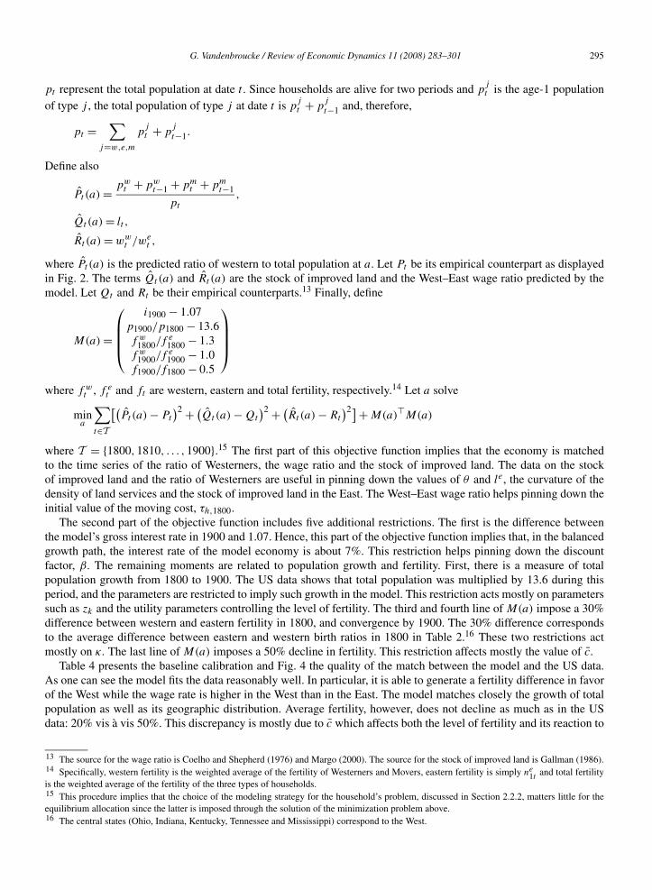
where T = {1800,1810, . . . ,1900}.15 The first part of this objective function implies that the economy is matchedto the time series of the ratio of Westerners, the wage ratio and the stock of improved land. The data on the stockof improved land and the ratio of Westerners are useful in pinning down the values of θ and le, the curvature of thedensity of land services and the stock of improved land in the East. The West–East wage ratio helps pinning down theinitial value of the moving cost, τh,1800.

The second part of the objective function includes five additional restrictions. The first is the difference betweenthe model’s gross interest rate in 1900 and 1.07. Hence, this part of the objective function implies that, in the balancedgrowth path, the interest rate of the model economy is about 7%. This restriction helps pinning down the discountfactor, β. The remaining moments are related to population growth and fertility. First, there is a measure of totalpopulation growth from 1800 to 1900. The US data shows that total population was multiplied by 13.6 during thisperiod, and the parameters are restricted to imply such growth in the model. This restriction acts mostly on parameterssuch as zk and the utility parameters controlling the level of fertility. The third and fourth line of M(a) impose a 30%difference between western and eastern fertility in 1800, and convergence by 1900. The 30% difference correspondsto the average difference between eastern and western birth ratios in 1800 in Table 2.16 These two restrictions actmostly on κ. The last line of M(a) imposes a 50% decline in fertility. This restriction affects mostly the value of c̄.

Table 4 presents the baseline calibration and Fig. 4 the quality of the match between the model and the US data.As one can see the model fits the data reasonably well. In particular, it is able to generate a fertility difference in favorof the West while the wage rate is higher in the West than in the East. The model matches closely the growth of totalpopulation as well as its geographic distribution. Average fertility, however, does not decline as much as in the USdata: 20% vis à vis 50%. This discrepancy is mostly due to c̄ which affects both the level of fertility and its reaction to

13 The source for the wage ratio is Coelho and Shepherd (1976) and Margo (2000). The source for the stock of improved land is Gallman (1986).14 Specifically, western fertility is the weighted average of the fertility of Westerners and Movers, eastern fertility is simply ne

1tand total fertility

is the weighted average of the fertility of the three types of households.15 This procedure implies that the choice of the modeling strategy for the household’s problem, discussed in Section 2.2.2, matters little for theequilibrium allocation since the latter is imposed through the solution of the minimization problem above.16 The central states (Ohio, Indiana, Kentucky, Tennessee and Mississippi) correspond to the West.


Table 4Baseline calibration

Preferences β = 0.98, c̄ = 0.09, σ = 0.525, κ = 15Technology μ = 0.6, φ = 0.2, θ = 0.1, zk = 3.7, le = 0.02

Initial value Annual growth rate

zy 1.0 0.55% (1800-40) and 0.71% (1840-00)zx 1.0 0.55% (1800-40) and 0.71% (1840-00)zl 1.0 0.30% (1800-60) and 0.60% (1860-00)τx 1.06 −1.5%τh 0.07 −1.5%

the wage rate. One can see from Eq. (11) that larger values of c̄ imply, at the same time, larger fertility rates everythingelse equal, and faster decline in fertility in response to an increase in the wage rate. The constraint that populationmust be multiplied by 13.6, imposed in the objective function, pushes the minimization routine toward “low” valuesof c̄, reducing at the same time the magnitude of the decrease in fertility.

3.2. Counterfactual experiments

The first experiment asks the following question: How did international immigration affect the US economy duringthe nineteenth century? To answer this question, the model is simulated under the calibration of Table 4, but with therate of international immigration, f , set to zero. Figure 5 presents the results of this experiment. Its main message isthat international immigration did not affect the US beyond its direct effect on population growth. Specifically, thebiggest departures from the baseline simulations are in panels B and D. Panel B represents the stock of improved landwhich increases less in the case where no immigrants came to the US than in the baseline case. Although the differenceis noticeable, one can argue that it is small. Panel D represents total population. Notice that fertility (panel C) is hardlyaffected by immigrants. To understand, observe that two forces are at work here. On the one hand, the absence ofimmigrants permits higher wages in the counterfactual economy and, hence, fertility tends to be lower. To be precise,the real wage rates in the counterfactual economy are initially identical to the those of the baseline economy. As timeunfolds, however, the difference in total population between the two economies increases, and the wage differenceincreases too. In 1900, the regional real wages in the counterfactual economy are 8% above their counterparts in thebaseline simulation (panel E). On the other hand, less population growth implies smaller regional densities (panel F)and, hence, higher fertility rates. Under the baseline calibration, the effects of these two opposing forces offset eachother.

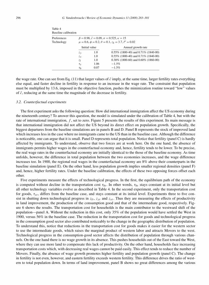
Five experiments measure the effects of technological progress. In the first, the equilibrium path of the economyis computed without decline in the transportation cost τht . In other words, τht stays constant at its initial level butall other technology variables evolve as described in Table 4. In the second experiment, only the transportation costfor goods, τxt , differs from the baseline case, and stays constant at its initial level. Experiments three to five con-sist in shutting down technological progress in zlt , zyt and zxt . Thus they are measuring the effects of productivityin land improvement, the production of the consumption good and that of the intermediate good, respectively. Fig-ure 6 shows the results. The transportation cost for households is the main contributor to the westward shift of thepopulation—panel A. Without the reduction in this cost, only 35% of the population would have settled the West in1900, versus 56% in the baseline case. The reduction in the transportation cost for goods and technological progressin the consumption good sector also contributed noticeably to the change in the geographic distribution of population.To understand this, notice that reductions in the transportation cost for goods makes it easier for the western sectorto use the intermediate goods, which raises the marginal product of western labor and attracts Movers to the west.Technological progress in the consumption-good sector affects the distribution of population through various chan-nels. On the one hand there is no wage growth in its absence. This pushes households out of the East toward the West,where they can use more land to compensate this lack of productivity. On the other hand, households face increasingtransportation costs which, with decreasing real wages cannot be paid easily. This effect tends to reduce the number ofMovers. Finally, the absence of wage growth promotes higher fertility and population growth (panel C). The changein fertility is not even, however, and eastern fertility exceeds western fertility. This difference drives the ratio of west-ern to total population down. In terms of land improvement, panel B shows no great differences among the various


Panels A, B and C display the model’s ability to fit the time series of the ratio of western to total population, the stock of improved land and theratio of western to eastern real wages, respectively. Panel D displays the model’s total population vis à vis its empirical counterpart. Panel E showsthe western and eastern fertility rates predicted by the model. Finally, panel F indicates the model’s ability to match the objectives in M(a).

Fig. 4. The model’s fit.

experiments. Yet, one can see that without technological progress in the consumption-good sector, the economy tendsto accumulate more land while, without decreasing cost of transportation, it tends to accumulate less.17

17 The importance of the transportation revolution for the development of the American economy has been emphasized earlier. See, for example,Fishlow (1965). Likewise, the work of Primack (1962) documents the extent of technological progress in the land-improvement sector and itsimpact on western development. However, neither Fishlow nor Primack present these phenomena in the context of a calibrated version of the


(A) (B)

(C) (D)

(E) (F)

A: share of westerners in the total population in the baseline calibration and the counterfactual experiment; B: stock of improved land; C: regionalfertility rates; D: total population; E: ratio of counterfactual wage rate to baseline wage rate in each region; F: density of population in each region.

Fig. 5. Counterfactual experiment—no international immigration.

The last experiment proposes an alternative land policy. What if the homestead act was never passed? Supposethat the US government sold raw land to the land-improvement sector, and contemplate the following price system.For u ∈ [lt , lt+1] the government charges qr

t (u) = qwt Λ(u) − ww

t /zlt and for u � lt+1, the government sets qrt (u) =

qrt+1(u)/it+1. Such a price function corresponds to what would have prevailed if land was traded on a competitive

market. The price set for u ∈ [lt , lt+1] corresponds to a zero-profit condition in the land improvement sector. Theprice set for u � lt+1 corresponds to a no-arbitrage condition. One can also interpret the zero-profit condition as the

optimal growth model. Herrendorf et al. (2006), to the contrary, propose a model of transportation and calibrate it to the US economy during thenineteenth. They use it to investigate regional trade patterns, though, rather than demographic changes.


(A) (B)

(C)Experiment 1: no technological progress in the transportation of labor; Experiment 2: no technological progress in the transportation of goods; Ex-periment 3: no progress in land-improvement technology; Experiment 4: no progress in consumption-good technology; Experiment 5: no progressin intermediate good technology.

Fig. 6. C ounterfactual experiment—no technological progress.

outcome of an auction process: land-improvement firms bid for the land until there is no profit to extract. Under thispolicy, the government’s transfer to a particular household is Tt = ∫ lt+1

ltqrt (u)du/(pw

t + pet + pm

t ). Figure 7 presentsthe result of this experiment. The main message, here, is that selling raw land instead of giving it out affects mostly thefertility rates (panel C), but is not enough to warrant significant changes in the stock of improved land (panel B) or thegeographic distribution of population (panel A). To understand this result, contemplate first the optimality conditionfor the land-improvement sector, Eq. (5). Under the baseline calibration, the price of raw land, qr

t (u), is set to zeroand, therefore, does not appear in the equation. Under the alternative policy, the price of raw land is not zero, but theno-arbitrage condition qr

t (lt+1) = qrt+1(lt+1)/it+1, implies that it drops out of the equation. In other words, under the

alternative policy the land-improvement firm cannot increase its value by reallocating purchases of raw land throughtime. Thus, in each case the pace of land accumulation depends on fundamentals only: technology and the qualityof the land. The value of the land-improvement firm is different in the two economies, though. This difference ischanneled, through transfers, to households and promotes an increase in fertility (panel C) hence faster populationgrowth (panel D). The latter fuels an additional demand for improved land (the opposite of the no-immigration case)but, quantitatively, this effect is small.18

4. Conclusion

During the nineteenth century the US experienced remarkable demographic changes. This paper proposed tomeasure how immigration and technological progress may have caused them. Despite its magnitude, the impact of

18 One interpretation is that, under the baseline price policy, the profit of the land improvement firm is taxed but not redistributed to households.If it were, the two experiments would yield exactly identical results.


(A) (B)

(C) (D)

Fig. 7. Counterfactual experiment—no homestead act.

international immigration turned out to be small compared to that of technology. On the one hand, immigrants sloweddown wage growth and hence promoted higher fertility inside the US. On the other hand they crowded the land whichturned out to offset the increase in fertility. In the end, the rate of natural increase in the US was barely affected. Tech-nological progress, through the transportation revolution and wage growth, had the biggest impact on the geographicdistribution of population and its rate of natural increase.

Acknowledgment

I am very thankful to Jeremy Greenwood for his support and guidance. I am also indebted to two anonymousreferees for useful comments. Finally, I would like to thank Mark Bils, Stanley Engerman and participants at the 2004SED meetings in Florence.

References

Atack, J., Bateman, F., Parker, W.N., 2000, Northern agriculture and the westward movement. In: Engerman and Gallman (2000).Benhabib, J., Rogerson, R., Wright, R., 1991. Homework in macroeconomics: Household production and aggregate fluctuations. Journal of Political

Economy 99 (6), 1166–1187.Coelho, P.R., Shepherd, J.F., 1976. Regional differences in real wages: The United States, 1851–1880. Explorations in Economic History 13 (2),

203–230.Easterlin, R.A., 1976. Population change and farm settlement in the Northern United States. Journal of Economic History 36 (1), 45–75.Engerman, S.L., Gallman, R.E., 2000. The Cambridge Economic History of the United States. Cambridge Univ. Press, Cambridge.Fishlow, A., 1965. American Railroads and the Transformation of the Ante-Bellum Economy. Harvard Univ. Press, Cambridge.Gallaway, L.E., Vedder, R.K., 1975. Migration and the old Northwest. In: Klingaman, D.C., Vedder, R.K. (Eds.), Essays in Nineteenth Century

Economic History: The Old Northwest. Ohio Univ. Press, Athens.


Gallman, R.E., 1986. The United States Capital Stock in the Nineteenth Century. Unpublished notes.Gallman, R.E., 1992. American economic growth before the Civil War: The testimony of the capital stock estimates. In: Gallman, R.E., Wallis, J.J.

(Eds.), American Economic Growth and Standards of Living before the Civil War. The Univ. of Chicago Press, Chicago.Gallman, R.E., 2000. Economic Growth and Structural Change in the Long Nineteenth Century. In: Engerman and Gallman (2000).Greenwood, J., Seshadri, A., 2002. The US demographic transition. American Economic Review 92 (2), 153–159.Greenwood, J., Seshadri, A., Vandenbroucke, G., 2005. The baby boom and baby bust. American Economic Review 95 (1), 183–207.Haines, M.R., 2000. The population of the United States, 1790–1920. In: Engerman and Gallman (2000).Herrendorf, B., Schmitz, J.A., Teixeira, A., 2006. Exploring the implications of large decreases in transportation costs. Mimeo.Margo, R.A., 2000. Wages and Labor Markets in the United States, 1820–1860. The Univ. of Chicago Press, Chicago.Mitchell, B.R., 1998. International Historical Statistics: The Americas, 1750–1993. Stockton Press, New York.O’Rourke, K.H., Williamson, J.G., 1999. Globalization and History, The Evolution of a Nineteenth-Century Atlantic Economy. MIT Press, Cam-

bridge.Primack, M.L., 1962. Farm formed capital in American agriculture, 1850–1910. PhD thesis. University of North Carolina.Yasuba, Y., 1962. Birth Rates of the White Population in the United States, 1800–1860, an Economic Study. Johns Hopkins University Studies in

Historical and Political Science 79th ser., vol. 2. Johns Hopkins Press, Baltimore.

The American frontier: Technology versus immigration - Guillaume

Documents

Transcript of The American frontier: Technology versus immigration - Guillaume