Final Document: AMSC/CMSC 663 and 664

The Alternating Direction Method of MultipliersAn ADMM Software Library

Peter Sutor, Jr.psutor@umd.edu

Project Advisor

Dr. Tom Goldsteintomg@cs.umd.edu

Assistant ProfessorDepartment of Computer Science

University of Maryland

May 15, 2016

Abstract

The Alternating Direction Method of Multipliers (ADMM) is a method that solvesconvex optimization problems of the form min(f(x) + g(z)) subject to Ax + Bz = c,where A and B are suitable matrices and c is a vector, for optimal points (xopt, zopt). It iscommonly used for distributed convex minimization on large scale data-sets. However,it can be technically difficult to implement and there is no known way to automaticallychoose an optimal step size for ADMM. Our goal in this project is to simplify theuse of ADMM by making a robust, easy-to-use software library for all ADMM-relatedneeds, with the ability to adaptively select step-sizes on every iteration. The librarywill contain a general ADMM method, as well as solvers for common problems thatADMM is used for. It also tries to implement adaptive step-size selection, have supportfor parallel computing and have user-friendly options and features.

Introduction

The generalization of ADMM’s usage is in solving convex optimization problems where the datacan be arbitrarily large. That is, we wish to find xopt ∈ X such that:

f(xopt) = min {f(x) : x ∈ X}, (1)

given some constraint Ax = b, where X ⊂ Rn is called the feasible set, f(x) : Rn 7−→ R isthe objective function, X and f are convex, matrix A ∈ Rm×n and vector b ∈ Rm. Our input xhere may have a huge amount of variables/dimensions, or an associated data matrix A for it cansimply be hundreds of millions of entries long. In such extreme cases, the traditional techniquesfor minimization may be too slow, despite how fast they may be on normal sized problems.

Generally, such issues are solved by using parallel versions of algorithms to distribute the work-load across multiple processors, thus speeding up the optimization. But our traditional optimizationalgorithms are not suitable for parallel computing, so we must use a method that is. Such a methodwould have to decentralize the optimization; one good way to do this is to use the Alternating Di-rection Method of Multipliers (ADMM). This convex optimization algorithm is robust and splitsthe problem into smaller pieces that can be optimized in parallel.

We will first give some background on ADMM, then describe how it works, how it is used tosolve problems in practice, and how it was implemented. Then, we discuss common problems thatADMM is used to solve and how they were implemented as general solvers in the ADMM library.Finally, we discuss our results on adaptive step-size selection and draw conclusions on the potentialfor this to be used in practice. We end by discussing potential future work on this solver libraryand adaptive step-sizes.

1

Background

In the following sections, we briefly describe the general optimization strategy ADMM uses,and the two algorithms ADMM is a hybrid of. For more information, refer to [1].

The Dual Problem

Consider the following equality-constrained convex optimization problem:

minx

(f(x)) subject to Ax = b (2)

This is referred to as the primal problem (for a primal function f) and x is referred to as theprimal variable. To help us solve this, we formulate a different problem using the Lagrangian andsolve that. The Lagrangian is defined as

L(x, y) = f(x) + yT (Ax− b). (3)

We call the dual function g(y) = infx(L(x, y)) and the dual problem maxy(g(y)), where y is thedual variable. With this formulation, we can recover xopt = arg minx(L(x, yopt)); f ’s minimizer.

One method that gives us this solution is the Dual Ascent Method (DAM), characterized atiteration k by computing until convergence:

1. x(k+1) := arg minx(L(x, y(k))) (minimization for f(x) on x)

2. y(k+1) := y(k) + α(k)(Ax(k+1) − b) (update y for next iteration)

Here, α(k) is a step size for the iteration k and we note that ∇g(y(k)) = Axopt − b, andxopt = arg minx(L(x, y(k))). If g is differentiable, this algorithm strictly converges and seeks outthe gradient of g. If g is not differentiable, then we do not have monotone convergence and thealgorithm seeks out the negative of a sub-gradient of −g. Note that the term yT (Ax− b) acts as apenalty function that guarantees minimization occurs on the given constraint.

Dual Decomposition

It’s important to realize that for high-dimensional input we may want to parallelize DAM forbetter performance. The technique for this is described in this section. Suppose that our objectiveis separable; i.e. f(x) = f1(x1) + · · · + fn(xn), and x = (x1, ..., xn)T . Then we can say the samefor the Lagrangian. From (3), we have: L(x, y) = L1(x1, y) + · · · + Ln(xn, y) − yT b, where Li =f(xi) + yTAixi. Thus, our x-minimization step in the DAM is split into n separate minimizationsthat can be carried out in parallel:

x(k+1)i := arg min

xi

(Li(xi, y

(k))).

This leads to a good plan for parallelization: disperse y(k), update xi in parallel then add up

the Aix(k+1)i . This is called Dual Decomposition (DD), and was originally proposed by Dantzig

2

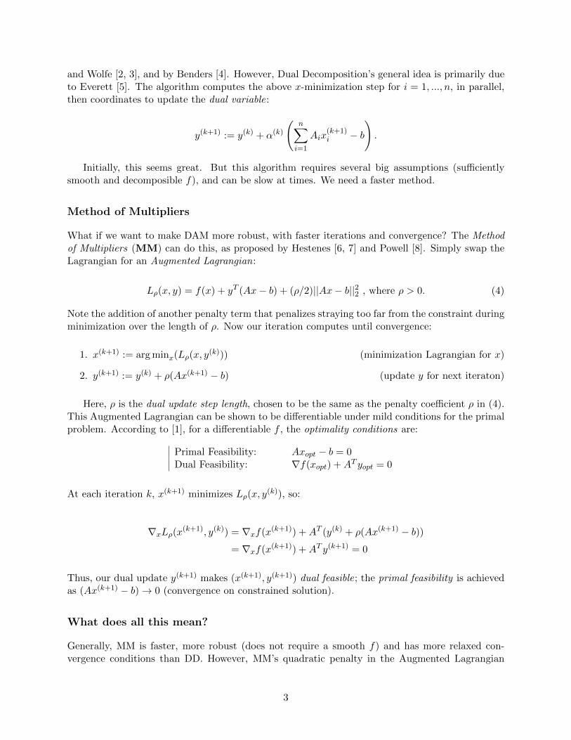
and Wolfe [2, 3], and by Benders [4]. However, Dual Decomposition’s general idea is primarily dueto Everett [5]. The algorithm computes the above x-minimization step for i = 1, ..., n, in parallel,then coordinates to update the dual variable:

y(k+1) := y(k) + α(k)

(n∑i=1

Aix(k+1)i − b

).

Initially, this seems great. But this algorithm requires several big assumptions (sufficientlysmooth and decomposible f), and can be slow at times. We need a faster method.

Method of Multipliers

What if we want to make DAM more robust, with faster iterations and convergence? The Methodof Multipliers (MM) can do this, as proposed by Hestenes [6, 7] and Powell [8]. Simply swap theLagrangian for an Augmented Lagrangian:

Lρ(x, y) = f(x) + yT (Ax− b) + (ρ/2)||Ax− b||22 , where ρ > 0. (4)

Note the addition of another penalty term that penalizes straying too far from the constraint duringminimization over the length of ρ. Now our iteration computes until convergence:

1. x(k+1) := arg minx(Lρ(x, y(k))) (minimization Lagrangian for x)

2. y(k+1) := y(k) + ρ(Ax(k+1) − b) (update y for next iteraton)

Here, ρ is the dual update step length, chosen to be the same as the penalty coefficient ρ in (4).This Augmented Lagrangian can be shown to be differentiable under mild conditions for the primalproblem. According to [1], for a differentiable f , the optimality conditions are:

Primal Feasibility: Axopt − b = 0Dual Feasibility: ∇f(xopt) +AT yopt = 0

At each iteration k, x(k+1) minimizes Lρ(x, y(k)), so:

∇xLρ(x(k+1), y(k)) = ∇xf(x(k+1)) +AT (y(k) + ρ(Ax(k+1) − b))= ∇xf(x(k+1)) +AT y(k+1) = 0

Thus, our dual update y(k+1) makes (x(k+1), y(k+1)) dual feasible; the primal feasibility is achievedas (Ax(k+1) − b)→ 0 (convergence on constrained solution).

What does all this mean?

Generally, MM is faster, more robust (does not require a smooth f) and has more relaxed con-vergence conditions than DD. However, MM’s quadratic penalty in the Augmented Lagrangian

3

prevents us from being able to parallelize the x-update like in DD. With this set-up, we cannothave the advantages of both MM and DD. This is where ADMM comes into play.

4

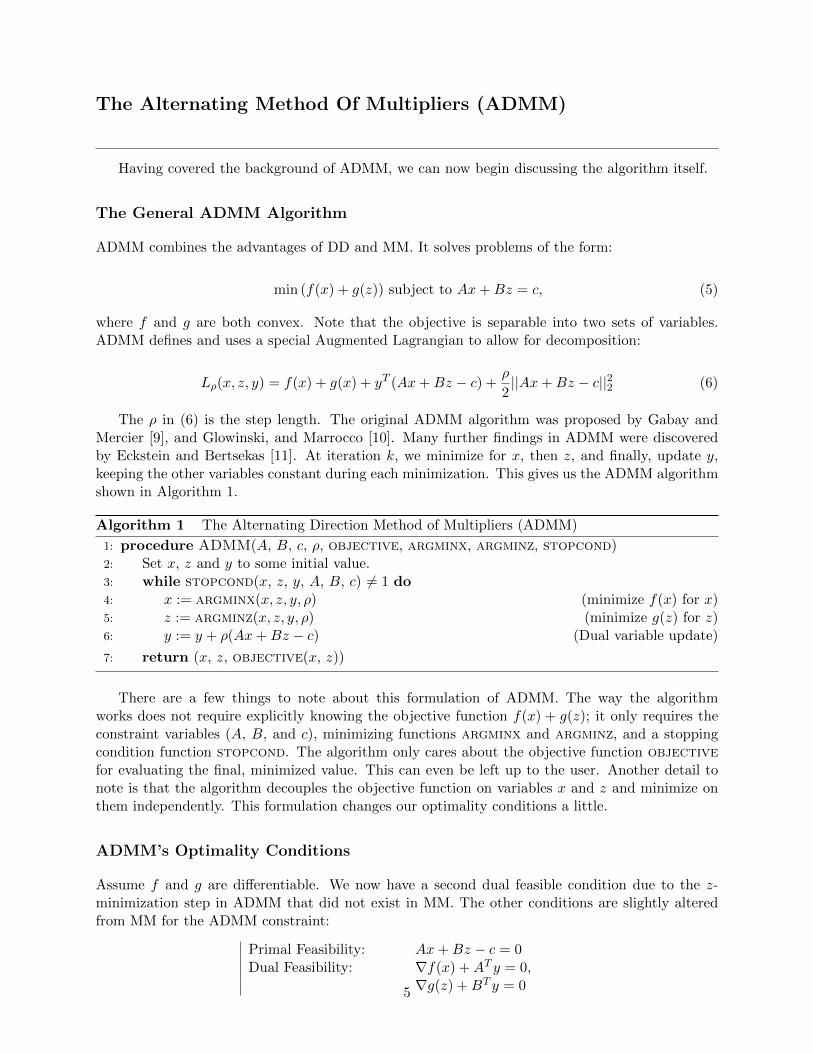
The Alternating Method Of Multipliers (ADMM)

Having covered the background of ADMM, we can now begin discussing the algorithm itself.

The General ADMM Algorithm

ADMM combines the advantages of DD and MM. It solves problems of the form:

min (f(x) + g(z)) subject to Ax+Bz = c, (5)

where f and g are both convex. Note that the objective is separable into two sets of variables.ADMM defines and uses a special Augmented Lagrangian to allow for decomposition:

Lρ(x, z, y) = f(x) + g(x) + yT (Ax+Bz − c) +ρ

2||Ax+Bz − c||22 (6)

The ρ in (6) is the step length. The original ADMM algorithm was proposed by Gabay andMercier [9], and Glowinski, and Marrocco [10]. Many further findings in ADMM were discoveredby Eckstein and Bertsekas [11]. At iteration k, we minimize for x, then z, and finally, update y,keeping the other variables constant during each minimization. This gives us the ADMM algorithmshown in Algorithm 1.

Algorithm 1 The Alternating Direction Method of Multipliers (ADMM)

1: procedure ADMM(A, B, c, ρ, objective, argminx, argminz, stopcond)2: Set x, z and y to some initial value.3: while stopcond(x, z, y, A, B, c) 6= 1 do4: x := argminx(x, z, y, ρ) (minimize f(x) for x)5: z := argminz(x, z, y, ρ) (minimize g(z) for z)6: y := y + ρ(Ax+Bz − c) (Dual variable update)

7: return (x, z, objective(x, z))

There are a few things to note about this formulation of ADMM. The way the algorithmworks does not require explicitly knowing the objective function f(x) + g(z); it only requires theconstraint variables (A, B, and c), minimizing functions argminx and argminz, and a stoppingcondition function stopcond. The algorithm only cares about the objective function objectivefor evaluating the final, minimized value. This can even be left up to the user. Another detail tonote is that the algorithm decouples the objective function on variables x and z and minimize onthem independently. This formulation changes our optimality conditions a little.

ADMM’s Optimality Conditions

Assume f and g are differentiable. We now have a second dual feasible condition due to the z-minimization step in ADMM that did not exist in MM. The other conditions are slightly alteredfrom MM for the ADMM constraint:

Primal Feasibility: Ax+Bz − c = 0Dual Feasibility: ∇f(x) +AT y = 0,

∇g(z) +BT y = 05

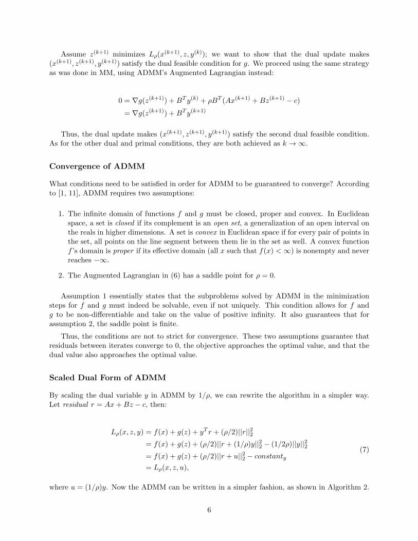
Assume z(k+1) minimizes Lρ(x(k+1), z, y(k)); we want to show that the dual update makes

(x(k+1), z(k+1), y(k+1)) satisfy the dual feasible condition for g. We proceed using the same strategyas was done in MM, using ADMM’s Augmented Lagrangian instead:

0 = ∇g(z(k+1)) +BT y(k) + ρBT (Ax(k+1) +Bz(k+1) − c)= ∇g(z(k+1)) +BT y(k+1)

Thus, the dual update makes (x(k+1), z(k+1), y(k+1)) satisfy the second dual feasible condition.As for the other dual and primal conditions, they are both achieved as k →∞.

Convergence of ADMM

What conditions need to be satisfied in order for ADMM to be guaranteed to converge? Accordingto [1, 11], ADMM requires two assumptions:

1. The infinite domain of functions f and g must be closed, proper and convex. In Euclideanspace, a set is closed if its complement is an open set, a generalization of an open interval onthe reals in higher dimensions. A set is convex in Euclidean space if for every pair of points inthe set, all points on the line segment between them lie in the set as well. A convex functionf ’s domain is proper if its effective domain (all x such that f(x) <∞) is nonempty and neverreaches −∞.

2. The Augmented Lagrangian in (6) has a saddle point for ρ = 0.

Assumption 1 essentially states that the subproblems solved by ADMM in the minimizationsteps for f and g must indeed be solvable, even if not uniquely. This condition allows for f andg to be non-differentiable and take on the value of positive infinity. It also guarantees that forassumption 2, the saddle point is finite.

Thus, the conditions are not to strict for convergence. These two assumptions guarantee thatresiduals between iterates converge to 0, the objective approaches the optimal value, and that thedual value also approaches the optimal value.

Scaled Dual Form of ADMM

By scaling the dual variable y in ADMM by 1/ρ, we can rewrite the algorithm in a simpler way.Let residual r = Ax+Bz − c, then:

Lρ(x, z, y) = f(x) + g(z) + yT r + (ρ/2)||r||22= f(x) + g(z) + (ρ/2)||r + (1/ρ)y||22 − (1/2ρ)||y||22= f(x) + g(z) + (ρ/2)||r + u||22 − constanty= Lρ(x, z, u),

(7)

where u = (1/ρ)y. Now the ADMM can be written in a simpler fashion, as shown in Algorithm 2.

6

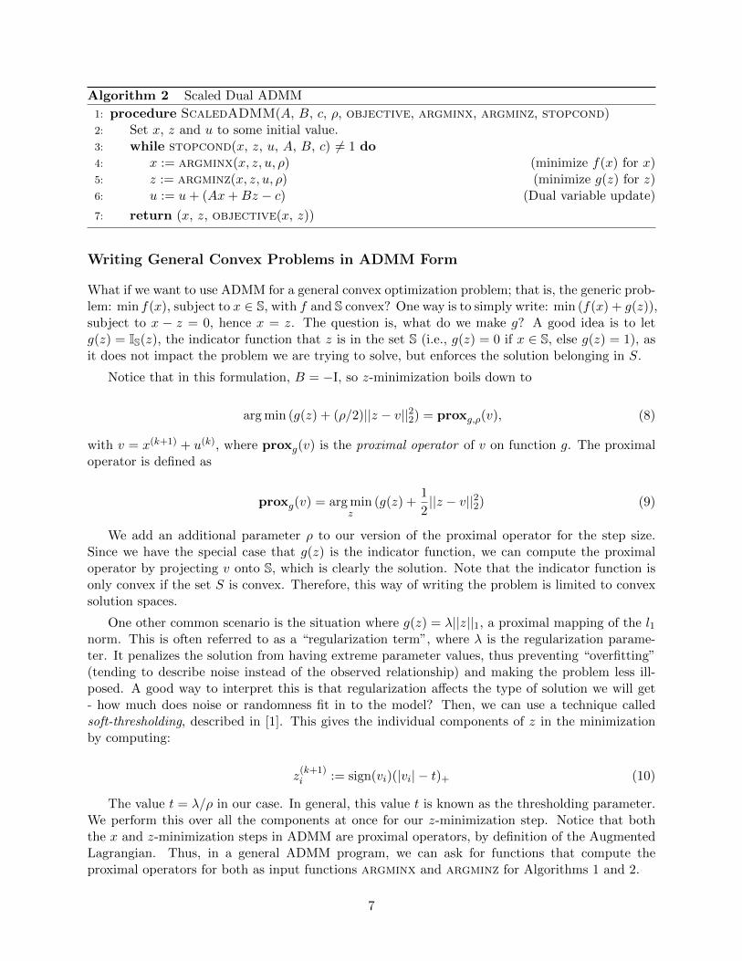
Algorithm 2 Scaled Dual ADMM

1: procedure ScaledADMM(A, B, c, ρ, objective, argminx, argminz, stopcond)2: Set x, z and u to some initial value.3: while stopcond(x, z, u, A, B, c) 6= 1 do4: x := argminx(x, z, u, ρ) (minimize f(x) for x)5: z := argminz(x, z, u, ρ) (minimize g(z) for z)6: u := u+ (Ax+Bz − c) (Dual variable update)

7: return (x, z, objective(x, z))

Writing General Convex Problems in ADMM Form

What if we want to use ADMM for a general convex optimization problem; that is, the generic prob-lem: min f(x), subject to x ∈ S, with f and S convex? One way is to simply write: min (f(x) + g(z)),subject to x − z = 0, hence x = z. The question is, what do we make g? A good idea is to letg(z) = IS(z), the indicator function that z is in the set S (i.e., g(z) = 0 if x ∈ S, else g(z) = 1), asit does not impact the problem we are trying to solve, but enforces the solution belonging in S.

Notice that in this formulation, B = −I, so z-minimization boils down to

arg min (g(z) + (ρ/2)||z − v||22) = proxg,ρ(v), (8)

with v = x(k+1) + u(k), where proxg(v) is the proximal operator of v on function g. The proximaloperator is defined as

proxg(v) = arg minz

(g(z) +1

2||z − v||22) (9)

We add an additional parameter ρ to our version of the proximal operator for the step size.Since we have the special case that g(z) is the indicator function, we can compute the proximaloperator by projecting v onto S, which is clearly the solution. Note that the indicator function isonly convex if the set S is convex. Therefore, this way of writing the problem is limited to convexsolution spaces.

One other common scenario is the situation where g(z) = λ||z||1, a proximal mapping of the l1norm. This is often referred to as a “regularization term”, where λ is the regularization parame-ter. It penalizes the solution from having extreme parameter values, thus preventing “overfitting”(tending to describe noise instead of the observed relationship) and making the problem less ill-posed. A good way to interpret this is that regularization affects the type of solution we will get- how much does noise or randomness fit in to the model? Then, we can use a technique calledsoft-thresholding, described in [1]. This gives the individual components of z in the minimizationby computing:

z(k+1)i := sign(vi)(|vi| − t)+ (10)

The value t = λ/ρ in our case. In general, this value t is known as the thresholding parameter.We perform this over all the components at once for our z-minimization step. Notice that boththe x and z-minimization steps in ADMM are proximal operators, by definition of the AugmentedLagrangian. Thus, in a general ADMM program, we can ask for functions that compute theproximal operators for both as input functions argminx and argminz for Algorithms 1 and 2.

7

This formulation allows us to solve problems of the form in (1). If there is already a constraintlike the one in (2), we can still use this formulation to solve it via ADMM. However, the constraintAx = b cannot simply be ignored; the parameters A and b will be incorporated into the x updatestep; i.e., they are part of the minimization problem for x (the solutions for which are supplied bythe user as a function in generalized ADMM). How to handle the x update is dependent on theproblem, though there are solutions for general cases such as in Quadratic Programming.

What about inequality constrained problems, such as Ax ≤ b? There are some tricks one cando to solve certain inequality constrained convex optimization problems. Using a slack variablez, we can write the problem as Ax + z = b, with z ≥ 0. This is now in ADMM form, but withthe additional constraint that z ≥ 0. The additional constraint primarily affects the z update stepin this case, as we need to ensure a non-negative z is chosen. Considering g(z) = λ||z||1, whichcan be solved in general via (10), we can modify the solution to select positive values for z. Forexample, we can project (10) into the non-negative orthant by setting negative components to zero,for v = Ax(k+1) + u(k).

Convergence Checking

The paper by He and Yuan in [12] constructs a special norm derived from a variational formulationof ADMM. Suppose you have a certain encoding of ADMM’s iterates in the form of

wi =[xi zi ρui

]T(11)

where xi, zi, and ui are iteration i’s results for x, z, and scaled dual variable u, and ρ is the stepsize. Let the matrix H be defined as follows:

H =

G 0 00 ρBTB 00 0 Im/ρ

(12)

where B ∈ Rm×n2 is the same matrix as from the ADMM constraints, Im is the identity of sizem, and G ∈ Rn1×n1 is a special matrix dependent on the variational problem ADMM is trying tosolve. Then, as shown in [12], {||wi − wi+1||2H} are monotonically decreasing for all iterations i:

||wi − wi+1||2H ≤ ||wi−1 − wi||2H (13)

The matrix G is actually irrelevant in this computation; it ends up disappearing anyway inthe end result. Thus, you do not need to know G to compute the H-norms. Since these normsmust be monotonically decreasing for ADMM to converge, evaluating and checking these normsevery iteration and checking the condition (13) is a good strategy to check that ADMM is actuallyconverging. For example, say you are given the constraints for an ADMM problem and the proximaloperators that correspond to them. If the proximal operators are incorrect, or the constraints do notmatch what the proximal operators compute, then it is not expected ADMM will actually converge.In such a case, checking (13) will tell you immediately if there’s an issue, and the algorithm canbe stopped, reporting an error. This avoids needlessly running what could be long and expensiveoperations that will not converge anyway.

Since the H-norms evaluations are not free (though they can be evaluated very quickly), thiswould likely be an option the user specifies when they are initially trying out proximal operators

8

for a problem. Also, as there is the concern of round-off error, the condition (13) would likely bechecked in terms of relative error to some specified (or default) tolerance.

Stopping Conditions

By [1], we can define the primal (p) and dual (d) residuals in ADMM at step k + 1 as:

pk+1 = Axk+1 +Bzk+1 − c (14)

dk+1 = ρATB(zk+1 − zk) (15)

The primal residual is trivial. However the dual residual stems from the need to satisfy the firstdual optimality condition ∇f(x) +AT y = 0. More generally, for subgradients ∂f and ∂g for f andg, and since xk+1 minimizes Lρ(x, z

k, yk):

0 ∈ ∂f(xk+1) +AT yk + ρAT (Axk+1 +Bzk − c)= ∂f(xk+1) +AT yk + ρAT (rk+1 +Bzk −Bzk+1)

= ∂f(xk+1) +AT yk + ρAT rk+1 + ρATB(zk − zk+1)

= ∂f(xk+1) +AT yk + ρATB(zk − zk+1)

So, one can say dk+1 = ρATB(zk+1 − zk) ∈ ∂f(xk+1) + AT yk, and the first dual optimalitycondition is satisfied by (15). It is reasonable to say that the stopping criteria is based on some sortof primal and dual tolerances that can be recomputed every iteration (or they could be constant,but adaptive ones are generally better). I.e., ||pk||2 ≤ εpri and ||dk||2 ≤ εdual. There are many waysto choose these tolerances. One common example, described in [1], where p ∈ Rn1 and d ∈ Rn2 :

εpri =√n1ε

abs + εrel max(||Axk||2, ||Bzk||2, ||c||2) (16)

εdual =√n2ε

abs + εrel||AT yk||2 (17)

where εabs and εrel are chosen constants referred to as absolute and relative tolerance. In practice,the absolute tolerance specifies the precision of the result, while the relative tolerance specifies theaccuracy of the dual problem in relation to the primal.

Another option for stopping conditions would be the H-norms used in convergence checking.The paper by He and Yuan in [12] also shows that the convergence rate of ADMM satisfies:

||wk − wk+1||2H ≤1

k + 1||w0 − w∗||2H (18)

for all solutions w∗ in the solution space of the problem. As a solution wk+1 for an ADMM problemmust satisfy ||wk − wk+1||2H = 0 (an extra iteration produced no difference), this implies that

||wk − wk+1||2H ≤ ε (19)

for some small, positive value ε is a good stopping condition for ADMM as well.

9

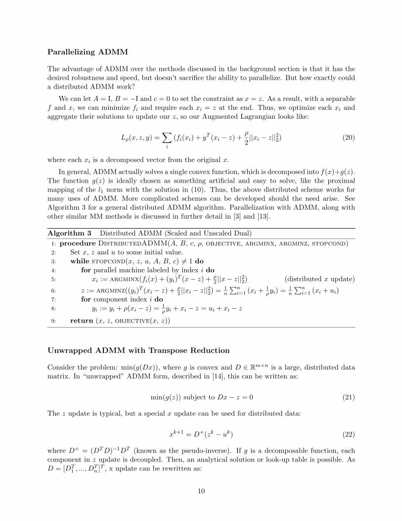
Parallelizing ADMM

The advantage of ADMM over the methods discussed in the background section is that it has thedesired robustness and speed, but doesn’t sacrifice the ability to parallelize. But how exactly coulda distributed ADMM work?

We can let A = I, B = −I and c = 0 to set the constraint as x = z. As a result, with a separablef and x, we can minimize fi and require each xi = z at the end. Thus, we optimize each xi andaggregate their solutions to update our z, so our Augmented Lagrangian looks like:

Lρ(x, z, y) =∑i

(fi(xi) + yT (xi − z) +ρ

2||xi − z||22) (20)

where each xi is a decomposed vector from the original x.

In general, ADMM actually solves a single convex function, which is decomposed into f(x)+g(z).The function g(z) is ideally chosen as something artificial and easy to solve, like the proximalmapping of the l1 norm with the solution in (10). Thus, the above distributed scheme works formany uses of ADMM. More complicated schemes can be developed should the need arise. SeeAlgorithm 3 for a general distributed ADMM algorithm. Parallelization with ADMM, along withother similar MM methods is discussed in further detail in [3] and [13].

Algorithm 3 Distributed ADMM (Scaled and Unscaled Dual)

1: procedure DistributedADMM(A, B, c, ρ, objective, argminx, argminz, stopcond)2: Set x, z and u to some initial value.3: while stopcond(x, z, u, A, B, c) 6= 1 do4: for parallel machine labeled by index i do5: xi := argminx(fi(x) + (yi)

T (x− z) + ρ2 ||x− z||

22) (distributed x update)

6: z := argminz((yi)T (xi − z) + ρ

2 ||xi − z||22) = 1

n

∑ni=1 (xi + 1

ρyi) = 1n

∑ni=1 (xi + ui)

7: for component index i do8: yi := yi + ρ(xi − z) = 1

ρyi + xi − z = ui + xi − z

9: return (x, z, objective(x, z))

Unwrapped ADMM with Transpose Reduction

Consider the problem: min(g(Dx)), where g is convex and D ∈ Rm×n is a large, distributed datamatrix. In “unwrapped” ADMM form, described in [14], this can be written as:

min(g(z)) subject to Dx− z = 0 (21)

The z update is typical, but a special x update can be used for distributed data:

xk+1 = D+(zk − uk) (22)

where D+ = (DTD)−1DT (known as the pseudo-inverse). If g is a decomposable function, eachcomponent in z update is decoupled. Then, an analytical solution or look-up table is possible. AsD = [DT

1 , ..., DTn ]T , x update can be rewritten as:

10

xk+1 = D+(zk − uk) = W∑i

Di(zki − uki ) (23)

Note that W = (∑

iDTi Di)

−1. Each vector Di(zki − uki ) can be computed locally, while only

multiplication by W occurs on central server. This technique describes another way to approachparallelizing ADMM in an efficient way, for certain problems.

Additionally, one can combine the strategy of Unwrapped ADMM with that of TransposeReduction. Consider the following problem:

minx

(1

2||Dx− b||22 +H(x)

)(24)

for some penalty term H(x). We know that:

1

2||Dx− b||22 =

1

2xT (DTD)x− xTDT b+

1

2||b||22 (25)

With this observation, a central server needs only DTD and DT b. For tall, large D, DTDhas much fewer entries. Furthermore, we can see that DTD =

∑iD

Ti Di and DT b =

∑iD

Ti bi.

Now, each server needs to only compute local components and aggregate on a central server. Thisis known as Transpose Reduction. Once the distributed servers compute DTD and DT b, we cancontinue on and solve the problem with Unwrapped ADMM, as described before. This strategyapplies to many problems; thus, many ADMM solvers for these problems can be optimized andwritten in an efficient, distributed method.

Fast ADMM

There exist faster converging strategies for ADMM, under certain conditions. The most inter-esting of these, due to their generality, are discussed in [15]. First, we will discuss Fast ADMM(FADMM), a technique to speed up convergence in the case of functions f and g being stronglyconvex. If a function h is strongly convex, then there exists a constant σh such that for every validx, y ∈ Rn in its domain:

〈p− q, x− y〉 ≥ σh||x− y||2 (26)

where p ∈ ∂h(x) and q ∈ ∂h(y). According to [15], the convergence for this type of problem canbenefit by using a predictor-corrector method where we predict a quadratically scaled progressionof the z and u variables in the next iteration, using this for the x, z and u updates. The predictiontakes advantage of the strong convexity, which guarantees that a function lies above its localquadratic approximation. This strategy is known as FADMM and the corresponding algorithm isshown in Algorithm 4.

As per the convergence proof in [15], FADMM’s predictors are used in the dual optimalitycondition, and thus the dual residual for stopping conditions in (15) must swap zk out for thepredicted value zk+1. Thus:

dk+1 = ρATB(zk+1 − zk+1) (27)

11

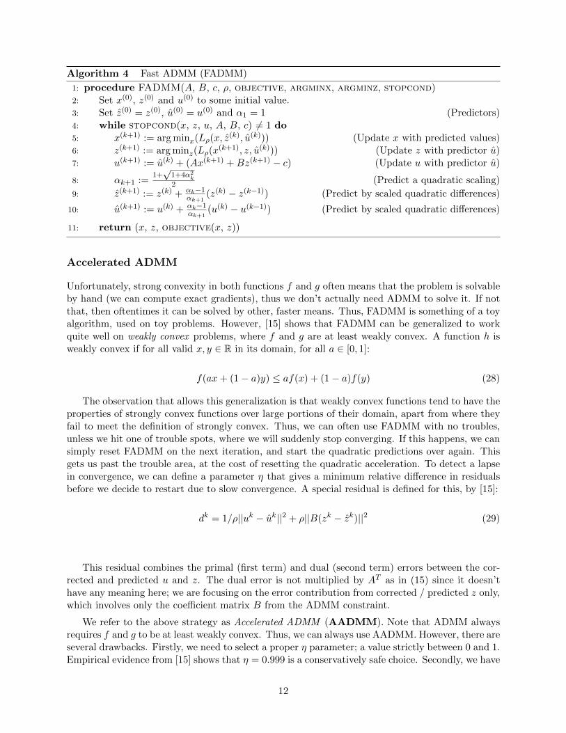
Algorithm 4 Fast ADMM (FADMM)

1: procedure FADMM(A, B, c, ρ, objective, argminx, argminz, stopcond)2: Set x(0), z(0) and u(0) to some initial value.3: Set z(0) = z(0), u(0) = u(0) and α1 = 1 (Predictors)4: while stopcond(x, z, u, A, B, c) 6= 1 do5: x(k+1) := arg minx(Lρ(x, z

(k), u(k))) (Update x with predicted values)6: z(k+1) := arg minz(Lρ(x

(k+1), z, u(k))) (Update z with predictor u)7: u(k+1) := u(k) + (Ax(k+1) +Bz(k+1) − c) (Update u with predictor u)

8: αk+1 :=1+√

1+4α2k

2 (Predict a quadratic scaling)

9: z(k+1) := z(k) + αk−1αk+1

(z(k) − z(k−1)) (Predict by scaled quadratic differences)

10: u(k+1) := u(k) + αk−1αk+1

(u(k) − u(k−1)) (Predict by scaled quadratic differences)

11: return (x, z, objective(x, z))

Accelerated ADMM

Unfortunately, strong convexity in both functions f and g often means that the problem is solvableby hand (we can compute exact gradients), thus we don’t actually need ADMM to solve it. If notthat, then oftentimes it can be solved by other, faster means. Thus, FADMM is something of a toyalgorithm, used on toy problems. However, [15] shows that FADMM can be generalized to workquite well on weakly convex problems, where f and g are at least weakly convex. A function h isweakly convex if for all valid x, y ∈ R in its domain, for all a ∈ [0, 1]:

f(ax+ (1− a)y) ≤ af(x) + (1− a)f(y) (28)

The observation that allows this generalization is that weakly convex functions tend to have theproperties of strongly convex functions over large portions of their domain, apart from where theyfail to meet the definition of strongly convex. Thus, we can often use FADMM with no troubles,unless we hit one of trouble spots, where we will suddenly stop converging. If this happens, we cansimply reset FADMM on the next iteration, and start the quadratic predictions over again. Thisgets us past the trouble area, at the cost of resetting the quadratic acceleration. To detect a lapsein convergence, we can define a parameter η that gives a minimum relative difference in residualsbefore we decide to restart due to slow convergence. A special residual is defined for this, by [15]:

dk = 1/ρ||uk − uk||2 + ρ||B(zk − zk)||2 (29)

This residual combines the primal (first term) and dual (second term) errors between the cor-rected and predicted u and z. The dual error is not multiplied by AT as in (15) since it doesn’thave any meaning here; we are focusing on the error contribution from corrected / predicted z only,which involves only the coefficient matrix B from the ADMM constraint.

We refer to the above strategy as Accelerated ADMM (AADMM). Note that ADMM alwaysrequires f and g to be at least weakly convex. Thus, we can always use AADMM. However, there areseveral drawbacks. Firstly, we need to select a proper η parameter; a value strictly between 0 and 1.Empirical evidence from [15] shows that η = 0.999 is a conservatively safe choice. Secondly, we have

12

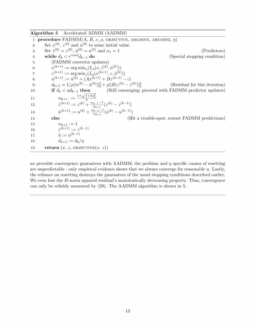
Algorithm 5 Accelerated ADMM (AADMM)

1: procedure FADMM(A, B, c, ρ, objective, argminx, argminz, η)2: Set x(0), z(0) and u(0) to some initial value.3: Set z(0) = z(0), u(0) = u(0) and α1 = 1 (Predictors)4: while dk < εresetdk−1 do (Special stopping condition)5: (FADMM corrector updates)6: x(k+1) := arg minx(Lρ(x, z

(k), u(k)))7: z(k+1) := arg minz(Lρ(x

(k+1), z, u(k)))8: u(k+1) := u(k) + (Ax(k+1) +Bz(k+1) − c)9: dk+1 = 1/ρ||u(k) − u(k)||22 + ρ||B(z(k) − z(k)||22 (Residual for this iteration)

10: if dk < ηdk−1 then (Still converging; proceed with FADMM predictor updates)

11: αk+1 :=1+√

1+4α2k

2

12: z(k+1) := z(k) +αk−1−1αk+1

(z(k) − z(k−1))13: u(k+1) := u(k) +

αk−1−1αk+1

(u(k) − u(k−1))14: else (Hit a trouble-spot; restart FADMM predictions)15: αk+1 := 116: z(k+1) := z(k−1)

17: u := u(k−1)

18: dk+1 := dk/η

19: return (x, z, objective(x, z))

no provable convergence guarantees with AADMM; the problem and η specific causes of resettingare unpredictable - only empirical evidence shows that we always converge for reasonable η. Lastly,the reliance on resetting destroys the guarantees of the usual stopping conditions described earlier.We even lose the H-norm squared residual’s monotonically decreasing property. Thus, convergencecan only be reliably measured by (29). The AADMM algorithm is shown in 5.

13

Implementing A General ADMM Function

The first step in our solver library is to have a generalized ADMM solver, which will be used tosolve more specific problems. Our goal was to make this solver as general as possible; i.e., it shouldonly be given proximal operator functions for f and g, and any customization to the algorithm. Itshould support all of the functionality from the previous section on ADMM, in a seamless way. Inthis section, we describe how this functionality is implemented and tested.

General Functionality

The generalized ADMM function, implemented in Matlab, accepts exactly 3 inputs: the proximaloperator for f , called xminf, the same for g, called zming, and a struct called options whichcontains fields that specify custom options for the execution of ADMM. Likewise, the output is astruct results that contains all the results for the execution of ADMM. This includes the final,optimal values for x, z, and u, the values of these at each iteration (in matrices/higher dimensionalarrays), the values of primal and dual residuals or H-norms at each iteration, predictors/residualsfor Accelerated/Fast ADMM at each iteration, ρ values at each iteration for adapative step-sizes,etc. All this information is recorded, if necessary, or desired. See the user manual for more detailson what is recorded.

Similarly, the user manual contains details on what fields can be set in options. These includestarting values for x, z and u, rho, parameters for residuals and stopping conditions (includingwhich ones to use), parameters for Accelerated/Fast ADMM, constraint data (A, B and c), thedimensions of these (rows m in c, columns nA and nB in A and B), and more. These optionsall have default values. Detection of existing fields and assignment of default values is done via auseful function setopts that selects fields and returns their values or defaults depending on if thesefields exist in options.

Proximal Operators

Proximal operators xminf and zming are function handles that must accept 4 inputs. In vanillaADMM, these inputs are as follows, respectively: x, z, u, and ρ. These are self-explanatory. De-manding these inputs for a proximal operator are somewhat counter-intuitive; typically a proximaloperator is expressed as accepting a vector v and proximal parameter t. Additionally, proximaloperators for a variable a normally don’t even use the current value of a! The reasoning behindusing 4 inputs is as follows.

• First of all, the user needs to know A, B and c (from ADMM’s constraint) in advance, thusit is redundant to, for example, compute and pass v = Bz − c+ u to xminf for an x update;the user can do it themselves when they define xminf in their local function (B and c canbe globally available in their local function). Perhaps the user doesn’t even need to multiplyB as it is equal to the identity, or c is the zero vector and doesn’t need to be added. Thus,the inputs x, z and u are sufficient, but still allow the user to make efficient improvements totheir proximal operators.

• Secondly, the parameter t often depends on ρ. If it does not, then it depends on some otherinformation that is unknown to general ADMM, and is encapsulated in the functionality ofthe proximal operator function handle.

14

• Third, if we are to use adaptive step sizes, and oftentimes proximal operators need to knowstep size ρ, we need to pass the current iteration k’s ρk to the proximal operators.

• Lastly, it’s possible that certain proximal operators cannot be computed precisely, but areestimated or utilize a predictor/corrector scheme. Since the only unique information thatADMM knows but the proximal operator doesn’t is x, z, and u, and estimation techniquesfor a proximal operator (say, for f) might be implicit (e.g., for f , they need the current x foran implicit definition), it makes sense to pass all this information.

Relaxation and Proximal Operators

There exists a common technique for improving convergence called relaxation, described in [1].Relaxation replaces the term Axk+1 in the updates for ADMM with:

Axk+1 := αAxk+1 − (1− α)(Bzk − c) (30)

where A, B and c are the constraint parameters for ADMM, and α is a user-provided parameterreferred to as the relaxation parameter. If α > 1, this is called over-relaxation, and if α < 1, thisis called under-relaxation. The value α ∈ (0, 2). Over-relaxation is the more common technique,with typical values of α being in the range [1.5, 1.8].

This technique interpolates Axk+1 with −(Bzk − c), which by the optimality conditions wouldmean that you allow g to contribute or detract from f ’s contribution to the ADMM constraint,without breaking the constraint. Tying these values to each other in such a way may provideattractive convergence properties, especially with over-relaxation, according to [11] and numericalresults from Eckstein in many other papers, mentioned in the over-relaxation section in [1].

This poses a drawback in proximal operators having the 4 inputs x, z, u, and ρ, as opposed tov and t, discussed in the prior section: we can’t perform relaxation. To get around this, if the userconsciously makes the decision to perform relaxation by specify a relax field in options (whichholds the value of α), we require that their proximal operators be designed to accept Ax, z, u, andρ. The value Ax here is the relaxed product Axk+1, given by (30).

A Model Problem For Testing

Since ADMM requires a problem to solve, we can only test it by using some kind of model problem,for which we can already find an analytic solution and for which the proximal operators are veryeasy to compute (no room for error). We choose the following model problem:

minx

(1/2||Px− r||2 + 1/2||Qx− s||2) (31)

where P,Q ∈ Rm×n and r, s ∈ Rm. Not only are the proximal operators for this problem easyto figure out, but one can solve this problem exactly by hand, allowing us to compare ADMM’ssolution to the exact solution. To compute the exact solution, we simply take the gradient of (31),set it equal to 0, and solve for x:

15

∇x(1/2||Px− r||2 + 1/2||Qx− s||2) := 0

P T (Px− r) +QT (Qx− s) := 0

P TPx+QTQx− (P T r +QT s) := 0

(P TP +QTQ)x := P T r +QT s

We see that then the minimizing x is:

x = (P TP +QTQ)−1(P T r +QT s) (32)

To efficiently compute this, we perform a Matlab system solve with the backslash operator,avoiding explicit computation of the inverse.

In ADMM form, we write problem (31) as:

min(1/2||Px− r||2 + 1/2||Qz − s||2), subject to x− z = 0 (33)

where f(x) is the first term and g(z) is the second. The Augmented Lagrangian is thus:

Lρ(x, z, u) = (1/2||Px− r||2) + (1/2||Qz − s||2) + ρ/2||x− z + u||2 (34)

To find the proximal operator for f and g here, we proceed as before and use gradients. For f ,we take the gradient of (34) for x:

∇xLρ(x, z, u) := 0

P T (Px− r) + ρ(x− z + u) := 0

P TPx+ ρx− P T r − ρ(z − u) := 0

(P TP + ρI)x := P T r + ρ(z − u)

Thus, our proximal operator for f is equal to computing:

x = (P TP + ρI)−1(P T r + ρ(z − u)) (35)

Following the same procedure for g, but with a gradient on z, we get the proximal operator:

z = (QTQ+ ρI)−1(QT s+ ρ(x+ u)) (36)

We will describe how to compute (35) and (36) efficiently in a later section about implementingADMM solvers for specific problems. The same goes for testing and validation results for the Modelproblem itself.

16

Implementing And Testing Convergence Checking

From (13), we can see that the following condition should hold for a converging ADMM:

||wi − wi+1||2H − ||wi−1 − wi||2H ≤ 0 (37)

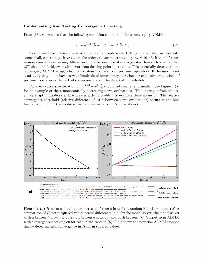
Taking machine precision into account, we can replace the RHS of the equality in (37) withsome small, constant positive εw, on the order of machine error ε, e.g. εw = 10−16. If the differencein monotonically decreasing differences of w’s between iterations is greater than such a value, then(37) shouldn’t hold, even with error from floating point operations. This essentially detects a non-converging ADMM setup; which could stem from errors in proximal operators. If the user makesa mistake, they don’t have to wait hundreds of unnecessary iterations or expensive evaluations ofproximal operators - the lack of convergence would be detected immediately.

For every successive iteration k, ||wk−1−wk||2H should get smaller and smaller. See Figure 1.(a)for an example of these monotonically decreasing norm evaluations. This is output from the ex-ample script hnormdemo.m, that creates a demo problem to evaluate these norms on. The relativeconvergence threshold (relative difference of 10−6 between norm evaluations) occurs at the blueline, at which point the model solver terminates (around 530 iterations).

Figure 1: (a) H-norm squared values across differences in w for a random Model problem. (b) Acomparison of H-norm squared values across differences in w for the model solver, the model solverwith a broken f proximal operator, broken g prox-op, and both broken. (c) Output from ADMMwith convergence checking on for each of the cases in (b). This shows the iteration ADMM stoppeddue to detecting non-convergence in H norm squared values.

17

To test the functionality of convergence checking, we use the example functionconvergencechecking.m, which creates a random problem for the Model solver to solve, and solvesit using the normal Model solver, a solver with a “broken” proximal operator for g, the same for abroken proximal operator f , and a solver with both of these errors in f and g’s proximal operators,outputting a graph comparing the H-norm squared evaluations between them. Figure 1.(b) showsthe resulting graph for the first 50 iterations of when the botched prox-op for f is (35) with (z+u)instead of (z − u), and the botched prox-op for g is (36) with a negative ρ(x + u) term instead ofa positive one. Note that if convergence checking is not on, the botched cases would perform thedefault maximum number of iterations (1000) due to stopping conditions never being reached, asthe botched cases do not converge.

We see that each of these cases have non monotonically convergent H-norm squared evaluationsnearly immediately, for mistakes in the proximal operators that could have occurred through simpletypos in the code. We expect from these results that ADMM will catch these problems nearinstantly. Figure 1.(c) shows the output for when convergence checking would stop ADMM’sexecution due to detecting non-convergence (single precision machine error 10−16 as the toleranceεw), in each case respective. For the botched g prox-op and the botched f prox-op cases, non-convergence is detected on the second convergence check (iteration 3, where checks start occurringat iteration 2). When both were botched, non-convergence was detected on the immediate firstcheck. Thus, Figure 1.(b)’s broken cases would not have made it past iteration 3, on the secondcheck, saving the user at least 997 needless iterations on a non-converging ADMM setup.

We test convergence checking in general ADMM by purposely botching proximal operators inthis way, for the Model problem, in various ways. We also do this for other solvers and get similarresults. The results indicate that not all erroneous changes cause non-convergence in ADMM. Forexample, botching the proximal operator for g in the model problem by adding a negative of theidentity, instead of the positive, does not break convergence if the random data in the correct prox-imal operator for f happens to perform a larger step towards the correct solution for the x-update.This negatively impacts convergence, but convergence does occur. Thus, convergence checking willnot catch ALL errors in proximal operators; only ones that break convergence. However, that istheir purpose, so this limitation does not affect the usefulness of convergence checking in general.Convergence checking should always be used by a user who is programming and testing their ownsolver, as it is cheap and can save them from crashing Matlab or waiting very long for non-converging executions of the solver. The only exception should be if they use Accelerated ADMMin their solver, as then we do not have the monotonically convergent guarantee.

Implementing Stopping Conditions

We have already outlined a couple of stopping conditions for ADMM in the section on StoppingConditions. Namely, we have two strategies for general stopping conditions:

1. The primal and dual residuals (14) and (15), along with adaptive tolerances for each, (16)and (17). We require that both conditions ||pk||2 ≤ εpri and ||dk||2 ≤ εdual be true for ADMMto be considered converged.

2. The H norm squared evaluations from (19). We require the relative condition, for some εH ,for iteration i ≥ 2, that:

||wi−1 − wi||2H − ||wi−2 − wi−1||2H ≤ εH ||wi−2 − wi−1||2H (38)

18

Tests of the convergence condition (19) have shown that the above formulation is the mostconvenient and general way of measuring relative error using H-norms.

In summary, the first strategy requires selection and tuning of εpri and εdual to get the precisionand accuracy desired in the resulting solution. However, the condition can be evaluated at anyiteration. The second condition is generally more conservative in measuring error, but requireschoosing only one parameter, εH . However, it can’t determine convergence until the second iterationdue to the reliance on the w values from the previous two iterations (w0 computed from startingvalues of x, z, and u).

We use the field stopcond in the options struct provided to ADMM for allowing the user todecide which stopping condition to use. This field can have the string values “standard”, to usethe first stopping condition, “hnorm” to use the second stopping condition, “both” to stop onlywhen both conditions are met, and “either” to stop if either condition is met. The default value is“standard”, if the user does not provide a choice for their stopping condition. For both conditions,we have additional fields for the parameters for each condition (abstol and reltol for εpri andεdaul, and Hnormtol for εH). They have their own default values if these are not specified.

Stopping conditions are extensively tested first by the Model problem solver, for correctness infunctionality. This is done by hand, changing values for fields in the options struct and observingthe effect on ADMM’s termination, to see if it matches the setting. Figure 1(a) shows an examplewith the Model problem of the second stopping condition in action, with the dashed line being thefinal value equal to (38) solved for εH that was required to break the condition. Once the stoppingcondition tests satisfied all cases in the Model problem, we expect that they will work for all othersolvers. This is supported by validation of results in those solvers and extensive testing throughtester functions for every solver. We will see more examples of the H-norm stopping condition, andthe standard one, in further sections, primarily where we show results for ADMM solvers of otherproblems.

Implementing Parallel ADMM

Algorithm 3 gives a clear method of implementing a Distributed form of ADMM. For ParallelADMM, we can simply use this strategy on local workers (cores and threads) on the machine viathe Matlab command parfor, which parallelizes a for loop’s execution over a number of workers.For a parallel x-update, ADMM defines a function that runs a parfor loop much as in steps 4-5of Algorithm 3. Likewise, there are such parallel functions for the z-update and u-update that canbe executed.

For a user to enable Parallel ADMM, they need to fill in the parallel field of the optionsstruct. The possible values are strings: “xminf”, for parallelizing only the proximal operator for f ;“zming”, for parallelizing only the proximal operator for g; “both” for performing parallel versionsof both, and “none” for not performing any parallel steps. The default value is “none”, if the userdoes not populate the parallel field. The u update is always parallel if the user specifies anyparallel functionality, as it would be a waste of resources to not distribute the workload of the uupdate across workers. If the user requires an alternate update for u (some parallelized problemsthat ADMM solves have very unique u-update steps), there also exists a field altu, which specifiesa function handle for an alternate u update that the user creates themselves. Furthermore, is theuser requires ADMM to perform some preprocessing of data before going into the main update loop,there exists a field preprocess that can be set to hold a function handle that will be executed withno inputs.

19

Parallel ADMM slices up the data in parallel update steps to distribute the workload acrossworkers. By default, it will split up the rows of the problem to solve as equally as it can among theavailable workers in the parallel pool. However, in the case of a single parallel proximal operator,there exists a field slices in the options struct that the user can populate with a vector thatcontains the number of rows to assign worker j at component j. If the user provides a single scalarvalue, the data is sliced up rows of that size, to the degree possible. Since the slices among theupdates can actually differ, then for the case of both proximal operators being parallel, the usercan instead provide a cell containing two column vectors of slice sizes, for f and g, respectively, asthe 1st and 2nd components of the cell. Each of these vectors follows the rules as stated for thesingle parallel proximal operator cases. In general, providing a scalar 0 instead of a vector for sliceswill revert Parallel ADMM to the default behavior of equally balancing the workload across theworkers.

For Parallel ADMM, we require that proximal operators add an additional parameter i as input,which should relay to the proximal operator which step i of the parfor loop is being executed.Since parfor can execute the proximal operator steps in non-sequential ways, we also require thatproximal operators make the slice of data needed to perform the parallel update available to theworker via parameter i, when using Parallel ADMM. If the user wishes to use parfor inside theirproximal operators, as opposed to letting ADMM handle it, the user has the ability to do thisin general. The aforementioned options struct field “parallel” can enable them to choose whichproximal operator should be parallelized by ADMM, and which shouldn’t be.

These ingredients in the options struct allow the user to fully customize their parallel executionof ADMM; either to be explicitly done by their own parfor loops inside of their proximal operators,or by ADMM, and gives the user control over how to distribute the data among the parallel workers.It also is built to require minimal input from the user to function; thus, a user can simply setparallel to “both” in the options struct and ADMM will automatically handle everything, if theirproximal operators are built to handle the additional slice i parameter.

One must note that there is a general overhead to initializing the parallel pools in Matlab.Depending on the machine and the number of cores, this can take a few seconds to half a minute.It is a one-time overhead, however, as parallel pools stay open for as long as needed in Matlab,depending on the customizable timeout parameter. We test and validate a parallel LASSO solverin future sections to test and validate the functionality of Parallel ADMM, as we need a specificproblem to solve. Additionally, the Unwrapped ADMM solver also uses parallel elements, and wetest and validate the functionality of that later as well.

Implementing Fast/Accelerated ADMM

Algorithms 4 and 5 give a pretty roadmap of how to implement Fast and Accelerated ADMM. Wesimply need to weave it together with vanilla ADMM’s execution in order to have a generalizedADMM that handles these faster convergent variants of ADMM. Note that Fast ADMM andAccelerated ADMM share the same basic predictor/corrector scheme and variables, but AcceleratedADMM requires a bit more for the reset stage, its special residual, and additional parameters. Inour ADMM method, we allow the user to enable faster ADMM by the field fast in the optionsstruct, which is a binary value. If true, ADMM will perform either Fast or Accelerated ADMM.The distinction between which of these is done by another field fasttype, which can hold the value“weak” or “strong”, which refer to the convexity of the problem ADMM is trying to solve. Bydefault, fasttype will always be “weak”, as all problems solvable by ADMM are weakly convex. If

20

the user really wants to try a toy problem with Fast ADMM, however, they can explicitly performit.

We implement the three varieties of ADMM (vanilla, fast, accelerated) by a case/if selection onthe steps that differ between them. The x, z and u updates have these cases on them, to updateaccording to the variant of ADMM being executed. The computation of the special residual in(29) is only performed and recorded if performing Accelerated ADMM, along with the reset steps.For Fast ADMM, we swap out the dual residual in standard stopping conditions for (27), andeverything else stays the same, in terms of stopping conditions. However, for Accelerated ADMM,the stopping conditions are overrided and the stopping condition in Algorithm 5 is used instead.Thus, for Accelerated ADMM, we have additional fields dvaltol and restart, which specify εreset

and η in Algorithm 5, respectively. By default, restart is set to 0.999, as recommended by [15].

Although we will not prove it here, the Model problem is strongly convex in both f and g.Thus, we can test FADMM and AADMM both using the Model problem solver. Furthermore, wecan validate the results by comparing the convergences between the vanilla, accelerated and fastvariants, which should be ranked from slowest to fastest converging, in this way. We show theresults for this in a later section, where we describe how each solver works, specifically in the Modelproblem section.

21

General Structure of the ADMM Library

With the implementation of the general ADMM function out of the way, we are poised todescribe the general structure of the ADMM library that was implemented in Matlab. Describingthis will make the testing and validation results for the solvers in the next major section easierto understand. The library is composed of 4 major parts; the main/root directory, the solverssub-directory, the testers sub-directory, and the examples sub-directory. We describe the contentsof each of these in the following sections. In general, the main/root directory has the most essentialfiles, the solvers directory has all of the solvers for general ADMM problems, the testers directoryhas all the testing and validation code for each solver, and the examples directory has assortedexamples of how to use the ADMM library, some of which also double for testing and validation ofcertain parts of general ADMM’s functionality.

The Main Directory

In the top-most level of the software library, we have the central files necessary for the overallfunctioning of the library. This, of course, includes our generalized ADMM method described inthe previous section, as a single file admm.m, as well as the sub-directories for solvers, testers and ex-amples. The main directory also has two complementary files, setuppaths.m and removepaths.m,used to set up and remove paths.

The function setuppaths is used to set up local paths to the other directories in the library;the solvers, testers, and examples sub-directories, so that the user can run any of the functions inthe library from any other directory. The user simply runs this function and the paths will be setup, assuming the names of ADMM’s sub-directories have not been altered. The function can alsobe given a binary quiet parameter, which specifies whether or not it should suppress output ofa message stating that the paths have been set up correctly. This function also defines and savesa global variable setup, which other functions in the library reference to see if the paths in thelibrary have been set up. Paths are persistent until the polar opposite function removepaths isexecuted, which removes any paths that have been set up for the library. It also has a optionalquiet parameter as setuppaths.

The main directory also contains a file showresults.m. This is a function, showresults, thatwill output information about a results struct returned by ADMM, or a test struct returned bya tester function. This function will also create plots about the execution of ADMM or a solver,that show salient information. This is, essentially, a convenience file for ADMM users to quicklyvisualize what happened when they executed admm or a solver.

Next, the main directory has a file errorcheck.m, which contains function errorcheck, ageneralized error checker of inputs to other functions. The purpose of this is to avoid redundanterror checks in solvers by simply calling this function to check if an input is valid or can be massagedinto a usable form (which is given as output), or create an error message if something is wrong.This function accepts an argument to error check, a string containing the type of check to perform,another string containing the name of this argument (used in error messages), and an optionaloptions struct that is used to customized the error checker in certain scenarios. The error-checkfunction can check if something is a matrix (square, or fat, or skinny), or if something is a vector(a row vector or column vector, massaging it into the correct type if it isn’t), or if something is anumber (positive real, nonnegative real, integer), or if something is a struct, or even more specific

22

checks, such as if something matches the form of the slices parameter in ADMM, creating sliceddata or information about slices from data in the options struct.

Finally, the main directory has the all-important file getproxops.m. The function getproxops

accepts a string, describing what problem to set up proximal operators for, and an argument struct,that contains arguments needed to create the proximal operator. It returns the proximal operatorsfor f and g, for the specified problem. This function, along with admm, is the work-horse of theADMM library, setting up instances of problems to solve and providing proximal operators for themfor all solvers and functions in the library. It consists of a massive switch statement that checks forwhat problem it should return a proximal operator for, then defines the prox-op functions withinitself, to act as a global instance from which the proximal operators access data when called byadmm’s updates. This function contains comments for each problem that describe it and how tosolve it with ADMM efficiently, also explaining how to arrive at the proximal operators for theproblem. The reason for such a set up is to conveniently have all proximal operators defined inone location (as some repeat or are very similar), and consolidate the code. It also can be usedby users that want to write their own versions of the solvers or add new proximal operators to itfor new problems (the function is built to scale up). A curious user can also simply look at howproximal operators are implemented or derived, in order to help them understand how the libraryworks, keeping all this information in once place for them.

The Solvers Subdirectory

This directory contains all of the ADMM library’s solvers. These are optimized functions that solvegeneral problems ADMM is used for. There are 11 solvers so far in the library, some of which alsocontain multiple versions of the same algorithm or parallel versions of it. Each of these solvers willbe discussed in the next major section, explaining the problem and how to arrive at a solution forit with ADMM. All testing and validation results are in this following section as well.

Generally, a solver accepts necessary inputs for its problem and an options struct that customizesboth its execution and that of the calls to ADMM that the solver will perform. These solvers aredesigned to be easy to use for a user. Each one has a special operation that will automaticallycall setuppaths to setup paths for the ADMM library, if necessary. Assuming the names of thelibraries folders are unchanged, the file name for setuppaths has not been changed, and the globalvariable setup created by setuppaths has not been altered, the paths will be silently set up forthe user.

The structure of these solvers is generally as follows:

1. Setup paths if necessary.

2. Check if no arguments have been provided. It will then create a demo test of itself using thesolver’s associated testing function in the testers folder.

3. Check the user input for error.

4. Set up the parameters for getproxops from user input, and create the arguments struct topass to getproxops

5. Call getproxops to instantiate the solver’s proximal operators.

6. Call admm on the proximal operators and report the results struct from its execution to theuser.

23

These functions are very short thanks to the work-horse efforts of admm and getproxops, alongwith the efforts of errorcheck. They demonstrate how quickly a user can write their own solverfor an ADMM problem using the library.

The Testers Subdirectory

Complementing the each solver in the solvers library is a tester function for the solver, used to bothtest it and validate the results. They generate random problems of a certain size, which are designedto be solvable by the associated solver. They then run the solver on this problem, and validatethe results against a “true” (or original) solution. These solvers generally accept a seed value forRNG (for repeatability and variety of tests), dimensions of the problem (rows and columns), anerror tolerance that specifies how far the solver’s solution can deviate from the original solution,a binary quiet variable that informs the tester whether or not to output and plot results of thetest, and an options struct that customizes the solver’s execution. The type of validation test foreach solver will be discussed in the next major section, showing the testing and validation resultsas well.

The structure of these solvers is generally as follows:

1. Setup paths if necessary.

2. Check if no arguments have been provided. It will then create a completely random demorun of itself using default values.

3. Check user input for any error.

4. Set up a random problem to solve for the solver, generally with a precomputed solution.

5. Run the solver.

6. Validate the results of the solver against the expected results.

7. If the error from the true solution is too high (relative to the specified error tolerance), reportthe test as a failure, otherwise a success.

8. Output or plot any results.

The testers folder also contains an additional file solvertester.m. This is a function solvertester

that will perform batches of tests over increasing scales for a solver. The purpose in doing this is tothoroughly test and validate the functionality of the solvers using the tester functions over a widespread of random data. The data scales itself over a parameter i, which denotes the size of the datain the tests. At each scale, a certain number of trials are performed using the testers, recording theaverage run time, any failures, and etc. This batch tester accepts as input a string containing thename of the solver to test, a minimum scale value imin, a maximum scale value imax, the numberof trials to perform at each scale, a binary value which denotes whether or not to show plots of theresults, and an options struct customizing the execution of the solver. This options struct can alsocontain fields that choose the seed for the RNG for the batch tester, the error tolerance to use in thetrials, the type of test to perform (e.g., scale over a square matrix, a fat matrix, a skinny matrix,etc.), a custom function handle scaler that accepts a scale i and outputs the problem sizes forthat scale. The batch tester aggregates the results of all trials over all scales, and returns a results

24

struct that contains a matrix of all trials (columns) and scales (rows) of tests performed, whetherthey were successful or not, etc. It also reports whether there were any failures. Ideally, this batchtester is used over reasonable scales and should report that all trials successfully converged withthe correct tolerance. This concludes the testing and validation for a solver.

The Examples Subdirectory

This subdirectory contain assorted examples of certain functionality of admm, and certain solvers.The purpose of this is to give examples of more concrete or complicated problems for solvers tosolve, and to show to a user how to use the solvers and admm. For our immediate purposes, theseserve as testing and validation of certain functionalities of admm and provide more testing andvalidation examples for certain solvers, to show that they are working as desired. The results ofthese functions will be shown in later sections, so we do not cover each file in detail here.

25

Solving, Testing and Validation of Solvers

Here we discuss some problems ADMM can solve, how to solve them efficiently, and describethe implementations of solvers. We also present the basic results of our testers and batch-testingon these solvers; i.e., our testing and validation for them.

The Model Problem

Recall that the Model problem (31) is what we use to validate and test function admm, our primarywork-horse for solving problems in ADMM. We already described how to solve it efficiently, andwhat the implementation would look like. We also described what it’s tester function would do(generate normally distributed, random matrices P and Q and vectors r and s) to set up an examplemodel problem, and what the true solution would be with (32). Here we present some testing andvalidation results on this problem to further demonstrate the correctness of admm.

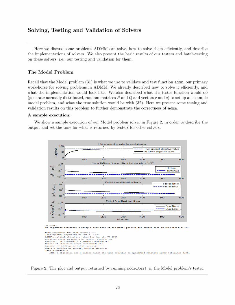
A sample execution:

We show a sample execution of our Model problem solver in Figure 2, in order to describe theoutput and set the tone for what is returned by testers for other solvers.

Figure 2: The plot and output returned by running modeltest.m, the Model problem’s tester.

26

The plots shown show the objective value converging to the true optimal objective value, andboth the H-norms and primal/dual norms reach their stopping thresholds as well. This indicatesthat ADMM itself is functioning correctly. The text output shows a low relative error between thetrue objective value and ADMM’s objective value, and a low value for the residual between thetrue minimizing x and the one ADMM computed. This validates that ADMM’s results are correctin the context of the Model problem.

Relaxation revisited:

Recall the technique of relaxation (30). We can test that it works correctly here by runningADMM repeatedly on different values of the relaxation parameter α. The quadratic form of themodel problem is one that would benefit from over-relaxation, so we expect to see that α > 1 willimprove the convergence. Figure 3 shows the changes in convergence of H-norm squared valueswith α and similar changes in the primal and dual residuals. These were obtained by running theexamples folder script relaxationexample.m. We see that as the relaxation parameter increases, sodoes the convergence speed of the Model solver. The relaxation functionality seems to be working,and over-relaxation does benefit the convergence, as predicted, validating our results for relaxation.

Figure 3: Differences in convergence of (left) H-norms squared values and (right) primal and dualresidual norms in the Model problem, over varying relaxation values.

FADMM and AADMM Comparison:

We can additionally test and validate our FADMM and AADMM implementations on the Modelproblem. In general, FADMM is much faster than AADMM, as restarts in AADMM can causea slow-down in convergence. However, Figure 4 shows an interesting scenario where this doesn’thold true. Here, normal ADMM doesn’t converge sufficiently (1000 iterations is the cutoff), whileFast takes about 400 iterations and Accelerated beats all with 200 iterations. We note that upto around 150 iterations, AADMM perfectly mirrors FADMM (no restarts). Then, it suddenlyconverges sharply to a solution. We attribute this to the restart that happens at the same time(restarts are recorded whenever they occur by admm). By the quadratic nature of the Model problem,AADMM hits a good spot to begin making quadratic predictions anew and outperforms FADMM.

27

Figure 4: (a) H-norm squared values between the 3 ADMM variants (b) Accelerated ADMM’sspecial residual norms (c) Primal and Dual residual norms for normal and Accelerated ADMM.

Additionally, note that H-norm squared values are no longer monotonically decreasing for AADMMand FADMM; this falls in line with the nature of these algorithms. We can clearly see the quadraticpredictions occurring via the wobbling of the residuals - even the primal and dual in Figure 4.(c).These results are obtained by the examples subdirectory function fasteradmmcomparison.

The Basis Pursuit Problem

Basis Pursuit is the problem of minimizing for x the objective function:

obj(x) = ||x||1, subject to Dx = s (39)

where D is a matrix and s is a column vector of appropriate length. This problem seeks todenoise a noisy signal x, for measurements s, using measurement data encoded into the rows of D.The xopt signal that is returned is the denoised signal. This is usually used in an underdeterminedsystem where we want the sparsest solution in the `1 sense. To write this problem into ADMM form,we note that the constraint Dx = s implies we require an x ∈ {v : Dv = s}. This is an indicatorproblem, where we can let f(x) be the indicator that x is not in this set. We let g(z) = ||z||1, andthen require x− z = 0, to tie x and z together - this is our ADMM constraint.

The proximal operator for g is easy; this is just soft-thresholding, from (10), with t = 1/ρ andv = x + u. The proximal operator for f is a bit more involved. We note that D is expected tobe underdetermined, and so we can’t directly solve Dx = s. Instead, we use a few tricks. Firstwe consider the matrix P = I − DT (DDT )−1D. Note that this matrix is algebraically equal to0. Also, we consider the vector q = DT (DDT )−1s, which is algebraically equal to D−1s. Then, aprojection of a vector v onto the set {v : Dv = s} is equivalent to x = Pv+q. For underdeterminedD, DDT is square and invertible. Thus, we cache DDT and use system solves to avoid computingits inverse directly. This allows us to compute and cache P and q, which are used to compute theminimizing x = Pv + q. Recall that since we chose f to be the indicator function, it will return 0(the minimum of f) for such an x. The vector v here is the parameter to the proximal operator.In general, for the proximal operator for f , in ADMM, v = −(Bz − c+ u). As B = −I and c = 0for Basis Pursuit in ADMM form, v = z − u.

28

By caching matrix P and vector q, we can quickly and efficiently compute x = Pv + q. Softthresholding is very efficient as well, for g’s proximal operator. The dominating overhead herewill be the one-time system solves we perform to compute P and q. Our solver basispursuit.m,accepts the parameters for Basis Pursuit, D and s, and an options struct to customize the callto admm. To test and validate basispursuit, our tester function creates a normally distributed,random D. It then randomly chooses a sparse, normally distributed x. We then simply computes = Dx. The resulting D and s are then passed to basispursuit. The tester expects the solverto minimize in the `1 sense, thus it expects the objective value to be much lower for xopt the solverdiscovers. The testers checks the condition that the value of (39)’s obj function has decreased. Itthen checks that ||Dxopt − s|| is very small. This validates the results of the solver.

Figure 5 shows the results of a sample execution of basispursuittest, the tester for solverbasispursuit. We see that denoised signal is indeed sparser in the `1 sense (less jumps than theoriginal from the baseline). The objective values reported by ADMM decrease below the originalsignal immediately on the first step. Although not shown, the norm ||Dxopt−s|| here is 6.3601e-14,nearing machine precision. These results indicate that Basis Pursuit is working as intended.

Figure 5: Results for a random test of our Basis Pursuit solver. We show the typical convergenceinformation (right) and the original signal vs. the denoised one returned by the solver (left).

The Least Absolute Deviations Problem

We now look at similar problem of minimizing in the `1 sense. Least Absolute Deviations (LAD)is defined by the problem of minimizing the objective:

obj(x) = ||Dx− s||1 (40)

This problem differs slightly from Basis Pursuit in that we do not have the constraint Dx = sanymore. We are given observation in the rows of D and corresponding noisy measurements s.Our goal here is to actually recover the original, minimal signal x, not denoise it, despite the noise

29

in s. We convert (40) trivially into ADMM form by letting f(x) = 0 and g(z) = ||z||1. By thesubstitution z = Dx− s, we have Dx− z = s, which is a constraint in ADMM form.

The proximal operators for LAD are very easy with this formulation. The one for g is simplythe soft-thresholding operator (10), once more, with t = 1/ρ and v = Dx− s+ u. Since f = 0, thegradient of the Augmented Lagrangian (7) collapses into:

∇Lρ(x, z, u) = DT (Dx− z − s+ u)

Setting this equal to 0 and solving it for x gives our minimizing x to be the solution to:

(DTD)x = DT (z + s− u) (41)

Instead of naively solving this system, we use a more efficient approach by finding the Choleskydecomposition RRT = DTD, where R and RT are lower and upper triangular, respectively. Weperform two easy system solves (due to R’s triangularity) by first finding a y such that Ry =DT (z + s− u) and then finding our minimizing x such that RTx = y.

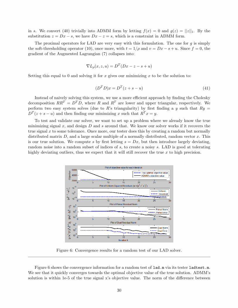
To test and validate our solver, we want to set up a problem where we already know the trueminimizing signal x, and design D and s around that. We know our solver works if it recovers thetrue signal x to some tolerance. Once more, our tester does this by creating a random but normallydistributed matrix D, and a large scalar multiple of a normally distributed, random vector x. Thisis our true solution. We compute s by first letting s = Dx, but then introduce largely deviating,random noise into a random subset of indices of s, to create a noisy s. LAD is good at toleratinghighly deviating outliers, thus we expect that it will still recover the true x to high precision.

Figure 6: Convergence results for a random test of our LAD solver.

Figure 6 shows the convergence information for a random test of lad.m via its tester ladtest.m.We see that it quickly converges towards the optimal objective value of the true solution. ADMM’ssolution is within 1e-5 of the true signal x’s objective value. The norm of the difference between

30

the true and recovered x is even lower, at 3.8234e-7 with an average error in a component evensmaller, at 2.6604e-8. These results are as expected from LAD; it solved the problem accuratelydespite highly deviating noise in s.

The Huber Fitting Problem

The Huber function is defined as:

huber(a) =

{a2/2 if |a| ≤ 1

|a| − 1/2 if |a| > 1(42)

For vector arguments, this is applied over the components of the vector. Suppose that we wantedto fit (42) to row data matrix D and measurement vector s. This problem can be defined asminimizing for x the objective function:

obj(x) = 1/2∑

(huber(Dx− s)) (43)

We can write (43) in ADMM form with the same trick as for LAD; set f(x) = 0 and g(z) =obj(z), such that Dx− z = s. The proximal operator for f is thus the same as LAD’s (41) and wecan use the same strategy to compute it efficiently. The proximal operator for g, however, is muchmore involved.

We see that (42) is smooth and its gradient can be computed piecewise as well. In the first case,the gradient of a2/2 is simply a. Thus, in this case the gradient of the Augmented Lagrangian forcomponent zi is:

zi − ρ([Dx]i − zi − si + ui)

Setting this equal to zero and solving it for zi gives:

zi = ρ/(1 + ρ)([Dx]i − si + ui) (44)

For the other case, the gradient of |zi| − 1/2 will be zi/|zi| = ±1, depending on the sign of zi.Solving for zi in this situation would give:

zi = ([Dx]i − si + ui) + (±1)/ρ

We can split these terms up into:

zi = ρ/(1 + ρ)([Dx]i − si + ui) + 1/(1 + ρ)([Dx]i − si + ui + (±1)(1 + ρ)/ρ) (45)

Comparing (44) and (45), we see the only difference is the second term in (45). If |zi| ≤ 1, thenthe second term is 0, otherwise it is there. If we let vi = [Dx]i − si + ui and t = (1 + ρ)/ρ, thensuch behavior on the second term’s vi + (±1)(1 + ρ)/ρ portion matches soft thresholding (10) forv and t. Thus, the z update can be written as:

z = ρ/(1 + ρ)v + 1/(1 + ρ)S(v, t) (46)

31

where v = Dx− s+ u, t = (1 + ρ)/ρ and S is the soft-thresholding operation.

Huber fitting essentially replaces sharp, absolute-value like points with a smooth quadratic tip.Thus, this sort of fitting is resistant to spikes in data, much like with LAD, although without theneed for sparsity.

The tester for huberfit sets up a normally distributed, random signal x. It then creates anormally distributed, random matrix D and normalizes the columns of it. Finally, a noisy vectors is created by computing Dx. We add sparse, but large noise to s. We expect that huberfit willnot be affected by these large spikes. We omit a demonstration of Huber Fitting as it is somewhatsimilar to LAD.

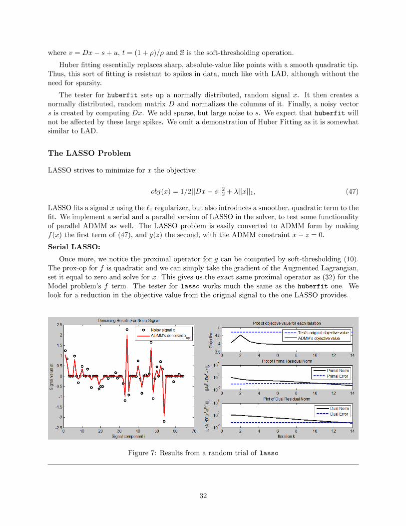
The LASSO Problem

LASSO strives to minimize for x the objective:

obj(x) = 1/2||Dx− s||22 + λ||x||1, (47)

LASSO fits a signal x using the `1 regularizer, but also introduces a smoother, quadratic term to thefit. We implement a serial and a parallel version of LASSO in the solver, to test some functionalityof parallel ADMM as well. The LASSO problem is easily converted to ADMM form by makingf(x) the first term of (47), and g(z) the second, with the ADMM constraint x− z = 0.

Serial LASSO:

Once more, we notice the proximal operator for g can be computed by soft-thresholding (10).The prox-op for f is quadratic and we can simply take the gradient of the Augmented Lagrangian,set it equal to zero and solve for x. This gives us the exact same proximal operator as (32) for theModel problem’s f term. The tester for lasso works much the same as the huberfit one. Welook for a reduction in the objective value from the original signal to the one LASSO provides.

Figure 7: Results from a random trial of lasso

32

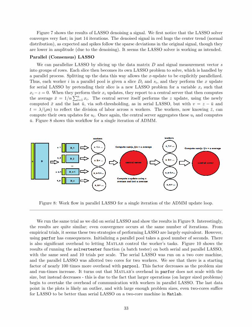
Figure 7 shows the results of LASSO denoising a signal. We first notice that the LASSO solverconverges very fast; in just 14 iterations. The denoised signal in red hugs the center trend (normaldistribution), as expected and spikes follow the sparse deviations in the original signal, though theyare lower in amplitude (due to the denoising). It seems the LASSO solver is working as intended.

Parallel (Consensus) LASSO

We can parallelize LASSO by slicing up the data matrix D and signal measurement vector sinto groups of rows. Each slice then becomes its own LASSO problem to solve, which is handled bya parallel process. Splitting up the data this way allows the x-update to be explicitly parallelized.Thus, each worker i in a parallel pool is given a slice Di and si, and they perform the x updatefor serial LASSO by pretending their slice is a new LASSO problem for a variable xi such thatxi−z = 0. When they perform their xi updates, they report to a central server that then computesthe average x = 1/n

∑ni=1 xi. The central server itself performs the z update, using the newly

computed x and the last u, via soft-thresholding, as in serial LASSO, but with v = z − u andt = λ/(ρn) to reflect the division of labor across n workers. The workers, now knowing z, cancompute their own updates for ui. Once again, the central server aggregates these ui and computesu. Figure 8 shows this workflow for a single iteration of ADMM.

Figure 8: Work flow in parallel LASSO for a single iteration of the ADMM update loop.

We run the same trial as we did on serial LASSO and show the results in Figure 9. Interestingly,the results are quite similar; even convergence occurs at the same number of iterations. Fromempirical trials, it seems these two strategies of performing LASSO are largely equivalent. However,using parfor has consequences. Initializing a parallel pool takes a good number of seconds. Thereis also significant overhead to letting Matlab control the worker’s tasks. Figure 10 shows theresults of running the solvertester function (a batch tester) on both serial and parallel LASSO,with the same seed and 10 trials per scale. The serial LASSO was run on a two core machine,and the parallel LASSO was allotted two cores for two workers. We see that there is a startingfactor of nearly 100 times more overhead with parpool. This factor decreases as the problem sizeand run-times increase. It turns out that Matlab’s overhead in parfor does not scale with thesize, but instead decreases - this is due to the fact that larger operations (on larger sized problems)begin to overtake the overhead of communication with workers in parallel LASSO. The last datapoint in the plots is likely an outlier, and with large enough problem sizes, even two-cores sufficefor LASSO to be better than serial LASSO on a two-core machine in Matlab.

33

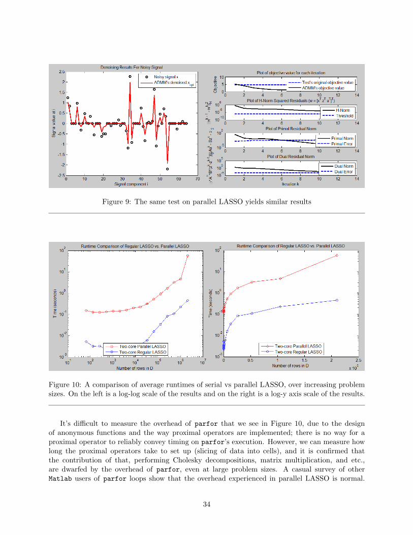
Figure 9: The same test on parallel LASSO yields similar results

Figure 10: A comparison of average runtimes of serial vs parallel LASSO, over increasing problemsizes. On the left is a log-log scale of the results and on the right is a log-y axis scale of the results.

It’s difficult to measure the overhead of parfor that we see in Figure 10, due to the designof anonymous functions and the way proximal operators are implemented; there is no way for aproximal operator to reliably convey timing on parfor’s execution. However, we can measure howlong the proximal operators take to set up (slicing of data into cells), and it is confirmed thatthe contribution of that, performing Cholesky decompositions, matrix multiplication, and etc.,are dwarfed by the overhead of parfor, even at large problem sizes. A casual survey of otherMatlab users of parfor loops show that the overhead experienced in parallel LASSO is normal.

34

Communication between workers (cores) is what slows down parfor. It is really only meant to beused when someone has at least 4 cores and is working with large datasets.

Unwrapped ADMM And The Linear SVM Problem

To test our general Unwrapped ADMM solver, and by proxy, our Linear SVM solver, we solvethe Linear SVM problem with Unwrapped ADMM. The Linear Support Vector Machine (SVM)problem strives to fit a loss function to a set of data D, such that it will generate a dividinghyperplane between classes, and thus create a general classifying hyperplane. In Unwrapped ADMMform, this problem can be formulated as:

obj(x) = 1/2||x||22 + C loss(Dx) (48)

where loss is a loss function and C is a constant, regularization parameter (enforcing strictness ofclassification). The smaller C is, the less of a hard margin exists on the classifying hyperplane.

We’ve already discussed how Unwrapped ADMM works, and a serial version is implementedexactly as described. The only thing left to discuss for the serial case is the proximal operator forg(z), which in this context is C loss(Dz). There are two types of common loss functions consideredfor Linear SVMs; the first is the 0-1 loss function, which is an indicator function of a component ofz being incorrectly classified. The second is the Hinge loss function, h(v) =

∑i(max(1 − `ivi, 0)),

where ` contains the training labels for classification. The Hinge loss function is a linear abstractionof the 0-1 (which is discontinuous), that is continuous and piece-wise differentiable. Thus, the Hingeloss is more used in practice. Its proximal operator in Unwrapped ADMM is:

z := (Dx+ u) + `T max(min(1− `T (Dx+ u), C/ρ), 0) (49)

In general, we cannot find a proximal operator for the 0-1 loss function. However, by transposereduction (25) in Unwrapped ADMM (23), we find that it is possible, as this technique makes rowsindependent of each other. We test our Linear SVM solver by having it classify points above a linex1 = x2 as +1 (correctly labeled) and below it as −1 (incorrectly labeled). The points are scatteredaround this dividing line randomly. A point that is supposed to be positive labelled will be placeda random distance away from x1 = x2, but above it, and vice versa for negative labelled points.These points are then randomly moved back towards x1 = x2 based on a separability parameter,to create some overlap of points that is nontrivial to separate linearly. Figure 11 shows an exampleof this test with separability parameter s = 0.2 (points get moved back randomly with coefficients on the random value between 0 and 1). We can visually see that the lines returned by both lossfunctions are close to the theoretically correct x1 = x2 line and each other.

We also have a harder testing and validation method for the Linear SVM solver; classificationof the MNIST hand-drawn digits. These are not entirely linearly separable, but should be closeenough such that a linear SVM will guess the correct digit with acceptable accuracy. A multi-class(more than 2) classifier with Linear SVMs can be trivially implemented by training the SVM oneach digit class, to distinguish between that digit and all others. Thus, we simply run linearsvm

10 times; once for each digit. We encode the handdrawn digits into row vectors by stacking thepixel rows of the image horizontally. They are 20 by 20 pixel images, thus we get vectors of length400. We have 60 thousand images at our disposal to choose training and testing subjects from, ofwhat size we please. Generally, it’s a good idea to have at least 5 times more training images thantesting images.

35

Figure 11: An example of a test of linearsvm. The dividing hyperplanes returned by the Hingeand 0-1 loss are both shown.

In Figure 12, we show the percentages of incorrectly guessed digits of each type over severalvarying classification runs with the Linear SVM solver on subsets of the MNIST data. We show theresults for both types of loss functions. In general, it seems that the linear classifier does a good jobfalling under 10% for almost all digits in the training stage, on both types of loss functions. We seein the top-left corner, that having a small sample under-represents the data and gives bad testingresults, despite the training results being seemingly good. The non-linear classification of thesehand written digits is evident when even going out to 2000 iterations and thousand of training andtesting samples doesn’t improve the results. We also observe that the 0-1 loss and Hinge loss havedifferent classification behaviors; sometimes the 0-1 loss does a much better job and sometimes itdoes not. All across the board, the digit 8 was the hardest to classify correctly in both the testingand training stages. This perhaps because of how similar hand-drawn 8’s can look to other digits,such as to 3’s, 0’s, 6’s, 9’s and 5’s. The Linear SVM clearly has trouble classifying 8’s correctlyduring the training stage and suffers for it in the testing stage.

Additionally, we also implemented a parallel version of Unwrapped ADMM. This implementsthe strategy (23) for updating x and the methods described there. Note that for UnwrappedADMM, the size of slices needs to be consistent across all sizes in order to build the matrix W .We tested how well parallel ADMM compares to its serial version in terms of performance usingparfor.

36

Figure 12: Several runs of the MNIST classifier, with varying iterations and training/testing subsetsizes.

Figure 13 shows our results for a batch test testing the average run-time performance of serialvs. parallel Unwrapped ADMM, over increasingly larger problems to solve. Once again, we seethe trend of the parallel version being roughly 100 times slower than the serial version for smallerproblems. However, these seem to converge quicker towards each other than in the Parallel LASSOcase, likely due to the Unwrapped ADMM technique being much efficient in parallel form. Beforehitting problems of scale 1 million, Parallel ADMM is only 10 times slower. It’s likely that forproblems of sizes in the millions, it would actually be faster to use parallel Unwrapped ADMM viaparfor loops on just two cores, than Matlab’s own multithreaded implementations. Given thetremendous overhead of parfor, this is actually somewhat impressive on the part of UnwrappedADMM with Transpose Reduction.

Honorable Mentions Among Solvers

We did not describe all the solvers I implemented here, nor all the strategies, in the interest ofspace. I also implemented solvers for Quadratic and Linear Programming problems, which are verysimilar to each other in implementation, but are also not very exciting to demonstrate any resultson. Furthermore, there is a solver for Sparse Inverse Covariance Selection, but I omitted discussionof that because (yet again) the results were not very interesting nor informative, but the problem,and the solution for it, were quite difficult to explain.

I also did not discuss the Total Variation Minimization (TVM) solver, which is a specific caseof the generalization of the LASSO problem where D = I and we apply a differencing scheme

37

Figure 13: On the left, a log-log plot of 2-core Parallel Unwrapped ADMM’s runtime vs. serialUnrapped ADMM’s runtime. On the right, a semi-log graph of this, showing the trends better.

on the x in the `1 regularization term. Solving this problem can be done very quickly as we’vealready collapsed D into the identity and can use convolutions/FFTs to help compute the solutionquickly, and the differencing scheme on the regularization term is sparse, and thus easier to dealwith. However, I implemented a solver for Total Variation early in the first semester and discussedin presentations at least twice, as well as describing it in the first progress document last semester,so I omitted rehashing it again here.

38

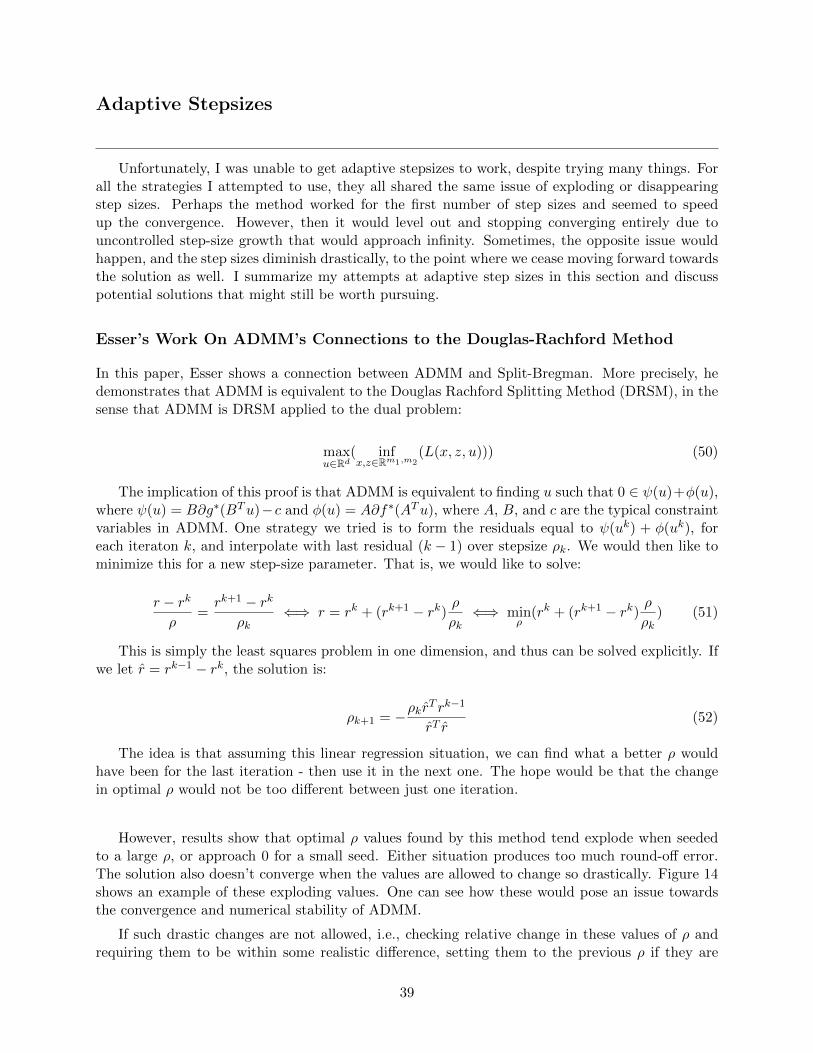
Adaptive Stepsizes

Unfortunately, I was unable to get adaptive stepsizes to work, despite trying many things. Forall the strategies I attempted to use, they all shared the same issue of exploding or disappearingstep sizes. Perhaps the method worked for the first number of step sizes and seemed to speedup the convergence. However, then it would level out and stopping converging entirely due touncontrolled step-size growth that would approach infinity. Sometimes, the opposite issue wouldhappen, and the step sizes diminish drastically, to the point where we cease moving forward towardsthe solution as well. I summarize my attempts at adaptive step sizes in this section and discusspotential solutions that might still be worth pursuing.

Esser’s Work On ADMM’s Connections to the Douglas-Rachford Method

In this paper, Esser shows a connection between ADMM and Split-Bregman. More precisely, hedemonstrates that ADMM is equivalent to the Douglas Rachford Splitting Method (DRSM), in thesense that ADMM is DRSM applied to the dual problem:

maxu∈Rd

( infx,z∈Rm1,m2

(L(x, z, u))) (50)

The implication of this proof is that ADMM is equivalent to finding u such that 0 ∈ ψ(u)+φ(u),where ψ(u) = B∂g∗(BTu)−c and φ(u) = A∂f∗(ATu), where A, B, and c are the typical constraintvariables in ADMM. One strategy we tried is to form the residuals equal to ψ(uk) + φ(uk), foreach iteraton k, and interpolate with last residual (k − 1) over stepsize ρk. We would then like tominimize this for a new step-size parameter. That is, we would like to solve:

r − rk

ρ=rk+1 − rk

ρk⇐⇒ r = rk + (rk+1 − rk) ρ

ρk⇐⇒ min

ρ(rk + (rk+1 − rk) ρ

ρk) (51)

This is simply the least squares problem in one dimension, and thus can be solved explicitly. Ifwe let r = rk−1 − rk, the solution is:

ρk+1 = −ρkrT rk−1

rT r(52)

The idea is that assuming this linear regression situation, we can find what a better ρ wouldhave been for the last iteration - then use it in the next one. The hope would be that the changein optimal ρ would not be too different between just one iteration.

However, results show that optimal ρ values found by this method tend explode when seededto a large ρ, or approach 0 for a small seed. Either situation produces too much round-off error.The solution also doesn’t converge when the values are allowed to change so drastically. Figure 14shows an example of these exploding values. One can see how these would pose an issue towardsthe convergence and numerical stability of ADMM.

If such drastic changes are not allowed, i.e., checking relative change in these values of ρ andrequiring them to be within some realistic difference, setting them to the previous ρ if they are

39

Figure 14: An example of the technique from (52) exhibiting the phenomenon of exploding step-sizes. This occurs 90 iterations into execution.

not, then adaptive ADMM seems to “work”. However, it doesn’t converge in less iterations asoften as it should. Sometimes it will converge in the same number of iterations as regular ADMM.Sometimes slightly less; rarely, even significantly less. On some occasions, it actually performs alittle worse (some low step-size values were chosen)! We would like to improve this performanceto consistently give significant lower iteration counts than a static step-size. Most of my efforts onadaptive step-sizes involved trying to fix this issue.

Using H-Norm Squared Values To Predict Stepsizes

Recall the w encodings (11), which, with the H matrix (12), define monotonically decreasingresiduals (13). These values provide some insight into the convergence of ADMM, as noted by [12],without needing to know anything more than the state of the ADMM iterates. These are a primecandidate for adaptive step sizes, since we can tell if ADMM is converging for a step-size if theystill decrease. Furthermore, if a change in step size does not break convergence, odds are that thechange aided convergence; especially if the differences between these values increase from it.

I spent a great deal of time just trying things out on various problems with this idea in mind.However, I kept running into the issue of inexplicably exploding or diminishing step sizes, much asin Figure 14. A future endeavor that might help with this is mapping out optimal step size pathsthrough brute force means. A first step in this direction is the function stepsizetesting, that canbe used to run multiple simultaneous executions of tester functions, on differing values of ρ. Thishelps to visualize the value of ρ actually affect convergence. For example, Figure 15 shows the effectof ρ on the convergence of the Total Variation Minimization solver. We see that decreasing ρ herewill strictly increase the convergence speed, up till a certain point (step sizes must be positive).On the flip side, problems like Sparse Inverse Covariance Selection give more ambiguous results, asshown in Figure 16. The iterations do not increase with ρ; the trials converge out of order.

40

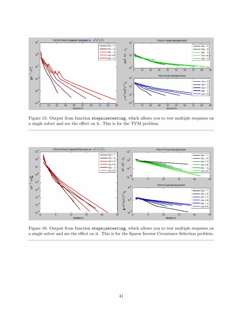
Figure 15: Output from function stepsizetesting, which allows you to test multiple stepsizes ona single solver and see the effect on it. This is for the TVM problem.

Figure 16: Output from function stepsizetesting, which allows you to test multiple stepsizes ona single solver and see the effect on it. This is for the Sparse Inverse Covariance Selection problem.

41

Future Work

There’s a lot of directions one can go in to improve the ADMM library:

1. Generalize the solvers to larger problems, then create less general solvers that use these. Forexample, a general solver for functions that use regularization terms. This would then beused by LASSO, Basis Pursuit, etc. Or, a general consensus ADMM setup.

2. More work on adaptive step sizes. There are bits and pieces of potential ways to make adaptivestep sizes that are actually somewhat useful. There’s a lot of potential in the H-norm squaredvalues, as they have properties tied directly to convergence that we could potentially abuse.There are also general schemes for choosing good values of ρ every iteration, but they rely onselection of other, sometimes multiple, parameters. Perhaps we can find a way to set theseparameters (maybe even every iteration) such that the step sizes are selected appropriately.

3. Add more options to the customizability of ADMM. For example, warm starting, the act of usingoptimal ADMM solutions from a previous run of a solver to speed up convergence of a currentrun. This would require a way for users to save and retrieve prior optimal values to warmstart whatever they would like for the next run. Also, options for disabling record-keeping ofdata during execution. I’ve noticed that batch testing really large problem sizes will quicklydrain memory when you record everything that happens.

4. Generalize admm.m to higher dimensional input. The values of x, z and u can be matrices, forexample. This is already done in the solver for Sparse Inverse Covariance Selection. However,constraint matrices A and B could be of higher dimension, such as 3-d matrices. Multiplyingmatrices would be an immediate issue.

5. Allow solvers to accept function handles instead of matrices, as well. Sometimes the con-straints for a problem are too big to directly put into a matrix, or perhaps it is inefficient todo so.

6. Try to see if there is a better way to create locally parallelized ADMM. Eventually, it would benice to scale up to distributed support for executing ADMM (e.g., message passing). However,Matlab might not be the best choice of language for this, given the slowness of the parfor

loop.

7. Implement a Python version, as was originally planned. This code should be able to reachthose who haven’t purchased Matlab or obtained it by some other means, as well.

42

Conclusion

The work that has been accomplished so far is a great basis for a very usable piece of software.The ultimate goal is to make solving problems with ADMM very easy to do, and more attractive forresearchers who may not have the programming skills or knowledge necessary to make their own,efficient implementations of proximal operators. Through my own efforts of programming thesesolvers, I’ve seen the usefulness of having a general admm function that can be customized to runas desired. Although the adaptive approach at step sizes has not yet produced much, it is a startto be able to at least sometimes achieve better convergence. In the future I hope to address theissue of exploding /disappearing step sizes and finally obtain a usable method for selecting goodstep sizes.

43

References

[1] S. Boyd, N. Parikh, E. Chu, B. Peleato, and J. Eckstein, “Distributed Optimization andStatistical Learning via the Alternating Direction Method of Multipliers”, Foundations andTrends in Machine Learning, vol. 3, no.1, pp. 1-122, 2010.

[2] G. B. Dantzig, Linear Programming and Extensions. RAND Corporation, 1963.

[3] G. B. Dantzig and P. Wolfe, “Decomposition principle for linear programs”, Operations Re-search, vol. 8, pp. 101-111, 1960.

[4] J. F. Benders, “Partitioning procedures for solving mixed-variables programming problems”,Numerische Mathematik, vol. 4, pp. 238-252, 1962.

[5] H. Everett, “Generalized Lagrange multiplier method for solving problems of optimum alloca-tion of resources”, Operations Research, vol. 11, no. 3, pp. 399-417, 1963.

[6] M. R. Hestenes, “Multiplier and gradient methods”, Journal of Optimization Theory andApplications, vol. 4, pp. 302-320, 1969.

[7] M. R. Hestenes, “Multiplier and gradient methods”, in Computing Methods in OptimizationProblems, (L. A. Zadeh, L. W. Neustadt, and A. V. Balakrishnan, eds.), Academic Press, 1969.

[8] M. J. D. Powell, “A method for nonlinear constraints in minimization problems”, in Optimiza-tion, (R. Fletcher, ed.), Academic Press, 1969.

[9] D. Gabay and B. Mercier, “A dual algorithm for the solution of nonlinear variational problemsvia finite element approximations”, Computers and Mathematics with Applications, vol. 2, pp.17-40, 1976.

[10] R. Glowinski and A. Marrocco, “Sur l’approximation, par elements finis d‘ordre un, et laresolution, par penalisation-dualit’e, d’une classe de problems de Dirichlet non lineares”, RevueFrancaise d’Automatique, Informatique, et Recherche Operationelle, vol. 9, pp. 41-76, 1975.

[11] J. Eckstein and D. P. Bertsekas, “On the Douglas-Rachford splitting method and the proximalpoint algorithm for maximal monotone operators”, Mathematical Programming, vol. 55, pp.293-318, 1992.

[12] B. He, X. Yuan, “On non-ergodic rate of Douglas-Rachford alternating direction method ofmultipliers,” Numerishe Mathematik, vol. 130, iss. 3, pp. 567-577, 2014.

[13] A. Nedic and A. Ozdaglar, “Cooperative distributed multi-agent optimization”, in ConvexOptimization in Signal Processing and Communications, (D. P. Palomar and Y. C. Eldar,eds.), Cambridge University Press, 2010.

[14] T. Goldstein, G. Taylor, K. Barabin, and K. Sayre, “Unwrapping ADMM: Efficient DistributedComputing via Transpose Reduction”, CoRR, vol. abs/1504.02147, 2015.

[15] T. Goldstein, B. O’Donoghue, S. Setzer and R. Baranuik, “Fast Alternating Direction Opti-mization Methods”, SIAM Journal on Imaging Sciences, vol. 7, iss. 3, pp. 1588-1623, 2014.

[16] E. Esser, Applications of Lagrangian-Based Alternating Direction Methods and Connections toSplit Bregman, April 2009.

44