The Air Cargo Load Planning Problem
174
The Air Cargo Load Planning Problem Zur Erlangung des akademischen Grades eines Doktors der Ingenieurwissenschaften bei der Fakultät für Wirtschaftswissenschaften des Karlsruher Instituts für Technologie (KIT) genehmigte Dissertation von Dipl.-Inform. Felix Brandt Tag der mündlichen Prüfung: 13.09.2017 Hauptreferent: Prof. Dr. Stefan Nickel Korreferent: Prof. Dr. Kai Furmans
Transcript of The Air Cargo Load Planning Problem
The Air Cargo Load PlanningProblem
Zur Erlangung des akademischen Grades eines
Doktors der Ingenieurwissenschaften
bei der Fakultät für Wirtschaftswissenschaftendes Karlsruher Instituts für Technologie (KIT)
genehmigte
Dissertation
von
Dipl.-Inform. Felix Brandt
Tag der mündlichen Prüfung: 13.09.2017Hauptreferent: Prof. Dr. Stefan NickelKorreferent: Prof. Dr. Kai Furmans

This document is licensed under a Creative Commons Attribution-NonCommercial-NoDerivatives 4.0 International License (CC BY-NC-ND 4.0): https://creativecommons.org/licenses/by-nc-nd/4.0/deed.en

Abstract
Felix BrandtThe Air Cargo Load Planning ProblemA major operational planning problem in the air cargo industry is how to arrange cargoin an aircraft to fly safely and profitably. Therefore, a challenging planning puzzle has tobe solved for each flight. Besides its complexity, the planning is mostly done manuallytoday, which is a time consuming process with uncertain solution quality. The literatureon loading problems in an air cargo context is scarce and the term is used ambiguously fordifferent subproblems like selecting containers, packing items into containers, or loadingcontainers into aircraft. All of the presented models only focus on certain aspects of whatis in practice a larger planning problem. Additionally, some practical aspects have notbeen covered in the literature.In this work, we provide a comprehensive overview of the air cargo load planning problemas seen in the operational practice of our industrial partner. We formalize its require-ments and the objectives of the respective stakeholders. Furthermore, we develop andevaluate suitable solution approaches. Therefore, we decompose the problem into foursteps: aircraft configuration, build-up scheduling, air cargo palletization, and weight andbalance. We solve these steps by employing mainly mixed-integer linear programming.Two subproblems are further decomposed by adding a rolling horizon planning approachand a Logic-based Benders Decomposition (LBBD). The actual three-dimensional packingproblem is solved as a constraint program in the subproblem of the LBBD.We evaluated our approaches on instances containing 513 real and synthetic flights. Thenumerical results show that the developed approaches are suitable to automatically gen-erate load plans for cargo flights. Compared to load plans from practice, we could achievea 20 percent higher packing density and significantly reduce the handling effort in the aircargo terminal. The achieved costs of additional fuel burn due to aircraft imbalances andreloading operations at stop-over airports are almost negligible. The required runtimesrange between 13 and 38 minutes per flight on standard hardware, which is acceptablefor non-interactive planning.Cargo airlines can significantly profit from employing the developed approaches in theiroperational practice. More and especially the profitable last-minute cargo can be trans-ported. Furthermore, the costs of load planning, handling effort, and aircraft operationscan be significantly reduced.
i


Contents
Abstract i
1 Introduction 11.1 Problem statement . . . . . . . . . . . . . . . . . . . . . . . . . . . . . . . 21.2 Research questions . . . . . . . . . . . . . . . . . . . . . . . . . . . . . . . 21.3 Organization of the thesis . . . . . . . . . . . . . . . . . . . . . . . . . . . 3
2 Air cargo primer 52.1 Air cargo business . . . . . . . . . . . . . . . . . . . . . . . . . . . . . . . . 52.2 The cargo . . . . . . . . . . . . . . . . . . . . . . . . . . . . . . . . . . . . 82.3 Unit load devices . . . . . . . . . . . . . . . . . . . . . . . . . . . . . . . . 92.4 Modes of transport . . . . . . . . . . . . . . . . . . . . . . . . . . . . . . . 112.5 Airport processes . . . . . . . . . . . . . . . . . . . . . . . . . . . . . . . . 122.6 Summary . . . . . . . . . . . . . . . . . . . . . . . . . . . . . . . . . . . . 16
3 Air cargo load planning 173.1 Planning tasks . . . . . . . . . . . . . . . . . . . . . . . . . . . . . . . . . . 173.2 Stakeholders and objectives . . . . . . . . . . . . . . . . . . . . . . . . . . 183.3 Traditional planning practice . . . . . . . . . . . . . . . . . . . . . . . . . . 193.4 Challenges of current practice . . . . . . . . . . . . . . . . . . . . . . . . . 213.5 Summary . . . . . . . . . . . . . . . . . . . . . . . . . . . . . . . . . . . . 22
4 Aircraft configuration 234.1 Related literature . . . . . . . . . . . . . . . . . . . . . . . . . . . . . . . . 254.2 The Aircraft Configuration Model . . . . . . . . . . . . . . . . . . . . . . . 25
4.2.1 Input parameters . . . . . . . . . . . . . . . . . . . . . . . . . . . . 264.2.2 Decision variables . . . . . . . . . . . . . . . . . . . . . . . . . . . . 264.2.3 Constraints . . . . . . . . . . . . . . . . . . . . . . . . . . . . . . . 274.2.4 Objective . . . . . . . . . . . . . . . . . . . . . . . . . . . . . . . . 284.2.5 Model overview . . . . . . . . . . . . . . . . . . . . . . . . . . . . . 28
4.3 Summary . . . . . . . . . . . . . . . . . . . . . . . . . . . . . . . . . . . . 29
5 Build-up scheduling 315.1 Related literature . . . . . . . . . . . . . . . . . . . . . . . . . . . . . . . . 325.2 The Build-up Scheduling Model . . . . . . . . . . . . . . . . . . . . . . . . 33
5.2.1 Input parameters . . . . . . . . . . . . . . . . . . . . . . . . . . . . 335.2.2 Decision variables . . . . . . . . . . . . . . . . . . . . . . . . . . . . 345.2.3 Constraints . . . . . . . . . . . . . . . . . . . . . . . . . . . . . . . 345.2.4 Objective . . . . . . . . . . . . . . . . . . . . . . . . . . . . . . . . 36
iii

Contents
5.2.5 Model overview . . . . . . . . . . . . . . . . . . . . . . . . . . . . . 365.3 Summary . . . . . . . . . . . . . . . . . . . . . . . . . . . . . . . . . . . . 37
6 Air cargo palletization 396.1 Related literature . . . . . . . . . . . . . . . . . . . . . . . . . . . . . . . . 406.2 The Air Cargo Palletization Model . . . . . . . . . . . . . . . . . . . . . . 42
6.2.1 Parameters . . . . . . . . . . . . . . . . . . . . . . . . . . . . . . . 436.2.2 Decision variables . . . . . . . . . . . . . . . . . . . . . . . . . . . . 446.2.3 Constraints . . . . . . . . . . . . . . . . . . . . . . . . . . . . . . . 446.2.4 Objective . . . . . . . . . . . . . . . . . . . . . . . . . . . . . . . . 536.2.5 Model overview . . . . . . . . . . . . . . . . . . . . . . . . . . . . . 54
6.3 Summary . . . . . . . . . . . . . . . . . . . . . . . . . . . . . . . . . . . . 57
7 Weight and balance 597.1 Related literature . . . . . . . . . . . . . . . . . . . . . . . . . . . . . . . . 607.2 The Weight and Balance Model . . . . . . . . . . . . . . . . . . . . . . . . 61
7.2.1 Parameters . . . . . . . . . . . . . . . . . . . . . . . . . . . . . . . 627.2.2 Decision variables . . . . . . . . . . . . . . . . . . . . . . . . . . . . 637.2.3 Constraints . . . . . . . . . . . . . . . . . . . . . . . . . . . . . . . 637.2.4 Objective . . . . . . . . . . . . . . . . . . . . . . . . . . . . . . . . 687.2.5 Model overview . . . . . . . . . . . . . . . . . . . . . . . . . . . . . 68
7.3 Summary . . . . . . . . . . . . . . . . . . . . . . . . . . . . . . . . . . . . 70
8 Benchmark instances 718.1 The ACLPP data model . . . . . . . . . . . . . . . . . . . . . . . . . . . . 718.2 Analysis and insights into real world instances . . . . . . . . . . . . . . . . 738.3 Datasets . . . . . . . . . . . . . . . . . . . . . . . . . . . . . . . . . . . . . 82
8.3.1 Master data . . . . . . . . . . . . . . . . . . . . . . . . . . . . . . . 828.3.2 Generation of synthetic flights . . . . . . . . . . . . . . . . . . . . . 828.3.3 Scenarios . . . . . . . . . . . . . . . . . . . . . . . . . . . . . . . . 83
8.4 Performance indicators . . . . . . . . . . . . . . . . . . . . . . . . . . . . . 848.5 Summary . . . . . . . . . . . . . . . . . . . . . . . . . . . . . . . . . . . . 86
9 A sequential planning approach 899.1 Volume-and-weight-based aircraft configuration . . . . . . . . . . . . . . . 90
9.1.1 Preprocessing . . . . . . . . . . . . . . . . . . . . . . . . . . . . . . 909.1.2 Mixed-integer model . . . . . . . . . . . . . . . . . . . . . . . . . . 91
9.2 Rolling horizon build-up scheduling . . . . . . . . . . . . . . . . . . . . . . 939.2.1 Preprocessing . . . . . . . . . . . . . . . . . . . . . . . . . . . . . . 939.2.2 Mixed-integer model . . . . . . . . . . . . . . . . . . . . . . . . . . 949.2.3 Rolling horizon planning . . . . . . . . . . . . . . . . . . . . . . . . 97
9.3 Air cargo palletization . . . . . . . . . . . . . . . . . . . . . . . . . . . . . 989.3.1 Mixed-integer model for bin assignment (BinAssign) . . . . . . . . . 999.3.2 Constraint program for the 3D knapsack problem (CPPack) . . . . 1029.3.3 Logic-based Benders Decomposition . . . . . . . . . . . . . . . . . . 1079.3.4 Sliding window of item sizes . . . . . . . . . . . . . . . . . . . . . . 1099.3.5 Estimation of stowage loss . . . . . . . . . . . . . . . . . . . . . . . 110
iv

Contents
9.3.6 Overall procedure . . . . . . . . . . . . . . . . . . . . . . . . . . . . 1119.4 Weight and balance . . . . . . . . . . . . . . . . . . . . . . . . . . . . . . . 111
9.4.1 Preprocessing . . . . . . . . . . . . . . . . . . . . . . . . . . . . . . 1119.4.2 Mixed-integer model . . . . . . . . . . . . . . . . . . . . . . . . . . 113
9.5 Summary . . . . . . . . . . . . . . . . . . . . . . . . . . . . . . . . . . . . 116
10 Evaluation 11910.1 Implementation and testing environment . . . . . . . . . . . . . . . . . . . 11910.2 Preliminary parameter tuning . . . . . . . . . . . . . . . . . . . . . . . . . 120
10.2.1 Aircraft configuration . . . . . . . . . . . . . . . . . . . . . . . . . . 12010.2.2 Build-up scheduling . . . . . . . . . . . . . . . . . . . . . . . . . . . 12110.2.3 Palletization . . . . . . . . . . . . . . . . . . . . . . . . . . . . . . . 12310.2.4 Weight and balance . . . . . . . . . . . . . . . . . . . . . . . . . . . 128
10.3 Results of the sequential approach . . . . . . . . . . . . . . . . . . . . . . . 12910.4 Summary . . . . . . . . . . . . . . . . . . . . . . . . . . . . . . . . . . . . 137
11 Coordinated planning approaches 13911.1 Shipment-based aircraft configuration . . . . . . . . . . . . . . . . . . . . . 13911.2 Weight-and-balance-based aircraft configuration . . . . . . . . . . . . . . . 14311.3 Summary . . . . . . . . . . . . . . . . . . . . . . . . . . . . . . . . . . . . 148
12 Conclusion 15112.1 Summary . . . . . . . . . . . . . . . . . . . . . . . . . . . . . . . . . . . . 15112.2 Research questions . . . . . . . . . . . . . . . . . . . . . . . . . . . . . . . 15312.3 Future work . . . . . . . . . . . . . . . . . . . . . . . . . . . . . . . . . . . 15412.4 Outlook . . . . . . . . . . . . . . . . . . . . . . . . . . . . . . . . . . . . . 155
Bibliography 157
List of Figures 161
List of Tables 163
Glossary 165
v

1 Introduction“A recession is when you have to tighten your belt; depression is whenyou have no belt to tighten. When you’ve lost your trousers – you’re inthe airline business.”
— Sir Adam Thomson, founder of British Caledonian
The airline business is highly competitive. Over the past decades this fierce competitionhas lead to numerous innovations to utilize the most expensive assets, the aircraft, tothe maximum and to reduce costs wherever possible. Operations research has played animportant role in this process by providing theory and tools for creating flight and crewschedules, optimizing revenue management, and supporting many more application areas.Staying in the airline business today without such support is not imaginable.Besides the well-known passenger airline business, a lot of airlines also transport cargoand many passenger flights carry cargo next to baggage in their lower decks. Furthermore,as of 2015 there are around 1,770 large cargo-only aircraft operated by airlines worldwide(Crabtree et al., 2016). Although all these aircraft transport less than 1 percent of worldtrade tonnage, this accounts for around 35 percent of world trade by value (Crabtree et al.,2016). Albeit its economical importance, air cargo has gained far less R&D attention thanthe passenger airline business and therefore has considerable potential to be improved byapplying current technologies and developing new tools like decision support systems.One major operational problem present specifically in air cargo is how to arrange thecargo in an aircraft. At first, loading cargo into an aircraft might seem to be a simpletask. But, in reality the loading must be carefully planned. For each single flight anairline that transports cargo has to answer a set of delicate planning questions to operatesafely and profitably. And there are more challenges: Cargo rates have fallen by around35 percent over the last 20 years (Crabtree et al., 2014). Therefore, airlines must aimfor a high utilization of the aircraft on each flight. On the other hand, there is a soaringovercapacity in the air cargo market, see Murray (2016) and The Economist (2016), whichleads to historically low average load factors of the aircraft. Accordingly, airlines are forcedto also reduce their operating cost for ground handling and fuel wherever possible to stayin business.In the past, there have been a couple of scientific contributions addressing “air cargoloading” problems. However, the term is used ambiguously for different decisions to bemade in the load planning process. This ranges from selecting the containers to load(Mongeau and Bes, 2003), over solving three-dimensional packing problems (Paquay etal., 2016), to balancing the aircraft for fuel efficiency (Lurkin and Schyns, 2015). All ofthe presented models only focus on certain aspects of what is in practice a larger planningproblem. In this work, we consider the overall problem of operational load planning forairlines that transport cargo and therefore we coin the term Air Cargo Load PlanningProblem (ACLPP).

1 Introduction
This work was partially supported by our industrial partner Lufthansa Cargo AG, thecargo division of the Lufthansa Group. Therefore, the described planning problems arederived from the current operational practice of our partner, but apply to other airlinestransporting cargo nonetheless. Besides an insight into practice and access to its planningexperts, our partner also provided benchmark data for the analysis of the problem at handand the evaluation of our approaches.
1.1 Problem statementAir cargo load planning today is often a manual task that has to be performed by experi-enced load planners (Amadeus, 2015). Only for parts of the planning process there existfirst commercially available decision support systems, like the SABLE Weight & Balancesystem (de Cleyn et al., 2014). Solving the full ACLPP in practice still involves a lot ofpen-and-paper or spreadsheet-based planning as well as trial and error during the actualpacking. On the one hand, this leads to high labor costs but often also to suboptimalresults, as there is a constant pressure of time and the problem complexity can be quitehigh.Accordingly, in today’s highly competitive air cargo market, the introduction of automateddecision support systems into the load planning process can provide a significant advantagefor airlines. First, by increasing the productivity of its load planning staff and also byproducing high quality solutions tailored for each individual flight.The aim of this thesis is to establish a comprehensive view of the load planning tasks in anair cargo terminal, collect the practical relevant aspects, formalize the underlying planningproblems, and develop suitable solution approaches. Our scope includes all the planningtasks regarding the cargo loading operations of a flight from the arrival of the individualshipments at the terminal up to the fully loaded and ready-to-go aircraft. Therefore, wefollow the planning processes seen in practice. Furthermore, we identify gaps betweenresearch and practice. In the end, we develop a decision support system for the ACLPPand two extensions for improving the solutions. Our goal is to achieve a solution qualitythat is competitive with the planning experts’ manual approach and can be computedwithin a reasonable amount of time on readily available commodity hardware. Ideally,this decision support system can then be used to provide the planners with good andfeasible solutions to start their day-to-day load planning tasks.
1.2 Research questionsTo structure our work, we follow three research questions:
1) What are the requirements and drivers of air cargo load planning in practice?In the literature, the term “air cargo loading” is used ambiguously and no general modelsexist. Therefore, we develop a unified nomenclature of the covered aspects and a compre-hensive model of the problem as seen in practice. We describe the decisions to be made,which restrictions have to be adhered, and what the overall objective is.
2

1.3 Organization of the thesis
2) Can valid and competitive load plans be generated with reasonable effort? De-scribing an optimization model is only halfway. We develop and implement a solutionapproach based on the current manual planning process of our industrial partner. There-fore, we split the problem into multiple steps and solve them one after the other. Weevaluate the approach on numerous test instances, stemming from real flights and ex-treme scenarios to get insights into the quality achieved and the runtimes required.
3) Does splitting the problem lead to adverse effects and what can we do about it?From a practical point of view, the steps performed during load planning should be asindependent and self-contained as possible. However, this limits the scope of optimization,which might lead to local optimization and to results that represent extreme cases. Thisin turn can lead to adverse results in the solution process. We analyze, where such effectsmay occur in our approach and develop ways to mitigate them.
1.3 Organization of the thesisFollowing the research questions outlined in the previous section we structure this thesisas follows:In Chapter 2 we provide a basic introduction and required background information aboutthe air cargo business. In Chapter 3 we focus on the loading aspects present in an aircargo environment. There, we introduce the Air Cargo Load Planning Problem, identifythe load planning stakeholders and their objectives in practice, and describe the currentplanning procedures and the related challenges.In the next four Chapters 4 to 7, we introduce the load planning problem and the relatedmodel in depth, accompanied by a review of the related literature. The respective chapterseach deal with a different subproblem: In Chapter 4 we describe the aircraft configura-tion, which selects the air cargo containers (ULDs) to use for each flight. In Chapter 5we introduce the build-up scheduling, which determines the starting time each ULD isassembled. In Chapter 6 we present the air cargo palletization, which distributes itemsacross ULDs and arranges the items in the ULDs. As the last subproblem, we describethe weight and balance in Chapter 7. It determines the arrangement of the assembledULDs in the aircraft.In Chapter 8 we introduce the benchmark instances that we use to evaluate our approach.Furthermore, we analyze the problem characteristics seen in practice and define perfor-mance indicators to measure the quality of a load plan.In Chapter 9 we present our main solution approach: SeqACLPP, a sequential planningapproach for the Air Cargo Load Planning Problem. We evaluate this approach in Chap-ter 10, discuss the results found, and identify areas for improvement. After that, wepresent our implementation of two extensions of the SeqACLPP approach and evaluatetheir performance in Chapter 11.In Chapter 12 we summarize the contributions of this work, discuss the results with regardto the considered research questions, and point out areas of future work.
3


2 Air cargo primerIn this chapter, we present a basic introduction into the world of air cargo and theoperational planning problems faced by airlines that handle cargo. The topics are selectedwith the required aspects of load planning in mind. In Section 2.1, we describe the businessof airlines that provide cargo services. Afterwards, we characterize the typical cargo inSection 2.2, the used loading devices in Section 2.3, the airlines’ modes of transportin Section 2.4, and the relevant airport processes in Section 2.5. For a more in depthintroduction we refer to the Air Cargo Guide by Grandjot et al. (2007).
2.1 Air cargo businessCargo airlines offer the very basic service to transport goods between different airportsat a certain price, very similar to the service provided by passenger airlines. But theworld of air cargo is more complex than it is for passengers. In Table 2.1, we sketch themain differences between the transport of passengers and cargo. In the remainder of thissection, we discuss these differences one by one.Besides the shipper and the airline, there is an important additional party in air cargo:the forwarder. He is typically involved in transporting the cargo from the original shipperto the departure airport and from the arrival airport to the consignee. Accordingly, theforwarders are by far the most important direct customers of a cargo airline, not theoriginal shippers. The market of forwarders is more concentrated than the airline market.This gives bigger forwarders a lot of power in negotiations. According to Burnson (2013),the six largest air cargo forwarders with their approximate market share as of September2013 are: DHL Global Forwarding (9.3%), DB Schenker (4.4%), Kuehne+Nagel (4.4%),Kintetsu World Express (4.3%), UPS Supply Chain Solutions (3.4%), and Panalpina(3.2%). Together they already represent nearly 30 percent of the global forwarding market.There is a range of different business models among airlines that offer cargo services. Themajority of airlines can be placed into one of these five categories:• Passenger airlines operate only passenger aircraft and sell the cargo capacity
in the lower deck that is not used for baggage. As this so-called belly space isquite limited and some goods are not allowed in there, cargo is more a by-productfor those airlines. Known carriers in this category include Delta Airlines, UnitedAirlines, or SAS Scandinavian Airlines. However, some passenger airlines, especiallylow-cost-carriers, even do not sell the free belly space. This way, they achieve shorterturn-around times at the airports and higher operational flexibility.• Integrated carriers, also called express carriers, combine the role of an airline
and the forwarder. Large carriers are for example DHL, UPS, FedEx, or TNT.They operate their own network of trucks, aircraft, and transition points. Thereby,

2 Air cargo primer
Passenger Air cargothe passenger is the customer a forwarder is an intermediary between
the airline and the customerstandard business model, sell seatson scheduled flights
diverse business models including ex-press, cargo-only, combination carriers
one seat, one passenger complex 3D puzzle of volume, weight,and handling requirements
active, passengers will watch for theirflight, board on their own, and contactstaff on problems
passive, all (un)packing has to be doneby airline staff, cargo will not notify any-body if it is forgotten
bidirectional flows, most passengerswill return to their origin
unidirectional flows, cargo flows arehighly imbalanced as cargo seldom re-turns to its origin
highly predictable, customers bookand pay months in advance
hard to predict, most bookings aremade at short notice, transport is usu-ally post-paid
Table 2.1: Main differences between the passenger airline and air cargo business
they provide a one-stop-shop solution for shippers. These carriers provide a morestandardized and automated service specifically designed for small shipments anddocuments. Therefore, these carriers usually apply limits on the maximum size,weight, and handling requirements of the shipments.• Combination carriers operate both passenger aircraft and cargo aircraft. Similar
to the passenger airlines, they transport cargo on their passenger aircraft as a by-product. However, they couple this service with their backbone network of cargo-only flights. This way, the smaller passenger flights can feed cargo into the cargo-only network to increase its overall utilization. Additionally, some combinationcarriers also provide trucking services, to transport cargo from/to smaller airportsthat are not serviced by cargo-only aircraft. Shipments in the cargo-only networkand trucking services can be of almost any size respecting the aircraft dimensionsand also contain hazardous goods. Carriers from this category often operate as aspecial cargo division of large airlines. Examples are Lufthansa Cargo, EmiratesSky Cargo, or Cathay Pacific Cargo.• Cargo-only carriers operate exclusively cargo aircraft. They have a significantly
smaller network than the combination carriers. Typically, they operate betweenlarge markets, like China and the USA, to fill their capacity. Thus, they leavethe main part of feeding and consolidation to their forwarders. Examples for largecargo-only carriers are Cargolux, AirBridgeCargo, or Nippon Cargo Airlines.• Charter carriers provide the most flexible and the most expensive air cargo trans-
portation service. With them, the shipper can transport nearly any good betweenany pair of airports as required by his own schedule. Therefore, these carriers are
6
2.1 Air cargo business
typically used for large machine parts, for example, power transformers or drillingequipment, or for emergency cases requiring an entire aircraft. There are few ded-icated charter carriers like Atlas Air, Southern Air, or Antonov Airlines, but mostother carriers will also offer their aircraft for charter.
This work mostly applies to combination and cargo-only carriers. The loading problemsfaced by the other types of carriers are usually easier to solve. The shipments transportedby express carriers and passenger airlines are mostly small, have little requirements, anddo not interfere with other shipments. Charter carriers often transport only a single bulkyitem or mostly homogeneous pallets, like in humanitarian aid.Besides the business models, the passenger and cargo business differ in several ways:In the passenger business one seat equates to one passenger. Managing the cargo capacityof a flight is much harder. To estimate the remaining cargo capacity, the airline hasto track weight, volume, and a variety of handling requirements, e.g., incompatibilitiesbetween shipments. Furthermore, it must solve a three-dimensional planning puzzle,defining how all items can be safely arranged inside the aircraft.Transporting air cargo involves extensive ground handling operations. First, the cargoneeds to be transported by conveyors or fork lifts inside the terminal. Furthermore, itmust be packed onto ULDs, lashed, and tracked on its way. Especially the packing partgets more difficult the more heterogeneous the cargo is.Another difference between the air cargo and passenger business is the geographic struc-ture of transport demands. Passenger flows are usually bidirectional as most passengersreturn to their origin. Therefore, passenger aircraft are typically operated as shuttles be-tween an airline’s hubs and other airports. In contrast, cargo flows are highly imbalancedand cargo airlines often operate flights with stop-overs, i.e., only a part of the payload is(un)loaded at a stop-over airport and the aircraft continues its journey under the sameflight number.To be able to describe certain subsections of a flight with stop-overs we define three termsthat appear frequently throughout this work. We define a flight as any sequence of aircraftmovements performed under the same flight number. A leg is a nonstop aircraft movementbetween two airports. A segment is a subsequence of legs of a flight on which cargo canbe transported. We note, that these terms are not used consistently in the airline world,but we stick to the above definitions for simplicity.Flights contain stop-overs mostly for two reasons. First, there might not be enough cargodemand between two airports to justify the use of a large cargo aircraft. By addingmore stop-overs in between, the airline can attract more shipments and thus increase theutilization of the aircraft. Lufthansa Cargo for example operates flight LH8272, depictedin Figure 2.1, from Frankfurt to Santiago de Chile with stop-overs in Dakar, Senegal, andViracopos, Brazil. The second reason is that splitting a long flight into two shorter legswith a stop-over for refueling allows the airline to load less fuel on each leg and insteadto load more cargo into the aircraft. In the latter case, the amount of loaded/unloadedcargo at the stop-over airports is usually smaller than in the former case. An exampleis the Lufthansa Cargo flight LH8475 from Hong Kong to Frankfurt with a 60 minutestop-over in Almaty, Kazakhstan, at half-distance.
7

2 Air cargo primer
FlightFRA DAK VCP SCL
FRA-SCL (LH8272)
Legs FRA-DAK4,641 km
DAK-VCP5,237 km
VCP-SCL2,555 km
Segments
FRA-DAKFRA-VCP
FRA-SCLDAK-VCP
DAK-SCLVCP-SCL
Figure 2.1: Illustration of the definition of flights, legs, and segments: Flight LH8272consists of three successive legs and technically cargo could be transported oneach of the six segments.
From a sales perspective, the air cargo business is split into two phases. In the firstphase, customers with a regular demand, typically forwarders, negotiate long-term con-tracts (LTC) with the airline. An LTC allows the customer to ship a certain amountof cargo on a defined set of flights for a fixed rate. This way, the airline increases itsplanning reliability and the customer gets a better price. Nevertheless, the actual cargothat will be on a flight is only booked a few days in advance. Depending on the contractthe customer is able to resign from a flight at short notice, sometimes even without anycost.The second phase of capacity sales is the regular booking process, which works similarto the one for passengers. The customer requests a quote, books capacity for a certainroute, and specifies the cargo properties like size, weight, and handling requirements.Most bookings only take place a few days before the flight, much shorter than in thepassenger business.To conclude, the air cargo business has some major differences to passenger airlines.Unidirectional cargo flows and late bookings make it hard to predict and plan ahead.When it comes to loading an aircraft, a lot of handling manpower is involved to solve acomplex three-dimensional planning puzzle in short time.
2.2 The cargo
The types of goods that are transported by air is manifold. Shipments can be anythingas small as a pocketbook, as large as an aircraft engine, or as long as the mast of a sailingvessel.Air cargo is a fast and safe way of transport and primarily attracts shipments that profitfrom these features. The transport by air is expensive, often 10 to 50 times the price of
8

2.3 Unit load devices
land transport. Therefore, it is usually only chosen for goods with at least one of thefollowing four properties:• urgent: The goods need to be at a distant place within short time. Typical goods
include spare parts, fashion, or living animals.• perishable: The goods degrade when they are not properly handled, for example
cooled. Therefore, they should be in a controlled environment and arrive at thedestination as fast as possible. Typical goods include flowers, drugs, or fresh food.• valuable: The goods are of high value and have to be transported in a secure way.
Typical goods include semiconductors, banknotes, or works of art.• dangerous: The goods may harm their environment when they are not properly
handled, which could mean tilting, too high surrounding temperature, or shock.Therefore, they have to be handled with care and the airline needs to be preparedfor accidents by training its crews and, for example, installing an automated fire-extinguishing system on the aircraft. Typical goods include chemicals, batteries, orradioactive materials.
Although some shipments can be quite small, a significant share of the cargo transportedby combination or cargo-only carriers is at least the size of a wooden pallet, like thosedefined in the ISO 6780 standard (ISO, 2003). Depending on the originating world regiontypical pallet sizes are 1,016x1,219 mm (North America), 800x1,200 mm (Europe), or1,100x1,100 mm (Asia) (Wikipedia, 2016). Throughout this work we refer to the Euro-pean pallet format 800x1,200 mm as EUR-pallet. Most shipments are box-shaped butirregular shapes, barrels, or just sacks occur frequently. Often multiple boxes are alreadyconsolidated onto a wooden pallet by the shipper and should not be separated by theairline. The packaging is often made of cardboard, wood, or styrofoam and optionallywrapped with plastic foil or protected by reinforced metal edges.Accordingly, one challenging task in load planning is to find a good combination of thesestrongly heterogeneous shipments to fill the aircraft capacity in a secure and efficient way.
2.3 Unit load devices
To streamline the ground handling processes, the cargo is most often assembled ontospecial air cargo pallets or containers, generally named unit load devices (ULD), see Fig-ure 2.2. Inside the aircraft the ULDs are placed on designated loading positions andlocked into position by latches on the floor. As the aircraft fuselage has a near circularcross section, there exist ULD types with different shapes to efficiently use the aircraft’sinterior space. Figure 2.3 shows a few frequently used ULD types.Tables 2.2 and 2.3 present popular types of ULDs, which can be loaded into many aircraft.However, most aircraft require certain types of ULDs for specific loading positions. Thereare general purpose ULDs, like plain aluminum pallets and containers of different formats,as well as special purpose ULDs for transporting cars, horses, or frozen goods.Pallets are generally preferred for larger shipments, because they can be easier packedthan containers and their contour can be freely chosen. It is also common to pack palletswith overhanging items to fill the full width of an aircraft’s lower deck. However, each
9

2 Air cargo primer
Figure 2.2: Loaded PMC pallet with main deck contour (left). Lower deck AKE container(right). Source: Lufthansa Cargo AG, Photographer: Stefan Wildhirt (left),Ingrid Friedl (right)
a) b) c) d)
Figure 2.3: Example ULD types in original proportions. Dashed lines mark the allowedcontour of a filled pallet while solid lines mark floor sheets and walls of con-tainers. a) main deck pallet (PMC) used in freighter aircraft b) lower deckpallet (PMC) and c) half-size lower deck container (AKE) used in freighter andwide-body passenger aircraft d) lower deck container (AKH) used in narrowbody passenger aircraft.
Type Volume Dimensions TareWidth Depth Height
AKH 3.6 m3 146-239 cm 144 cm 111 cm 85 kgAKE 4.3 m3 146-195 cm 142 cm 160 cm 66 kgALF 9.0 m3 305-400 cm 142 cm 160 cm 230 kgAMP 11.6 m3 223 cm 305 cm 154 cm 305 kgAMJ 16.5 m3 230 cm 306 cm 240 cm 320 kg
Table 2.2: Common ULD container types. The given dimensions are the usable spaceinside the ULD. Tare is the empty weight of the ULD.
10
2.4 Modes of transport
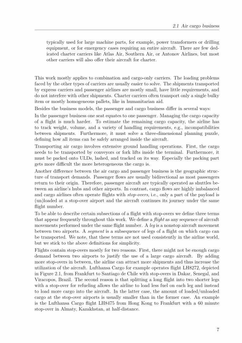
Type Width Depth Tare RemarksPAG 210 cm 304 cm 115 kg MD, or rotated 90◦ in LDPMC 230 cm 304 cm 115 kg MD, or rotated 90◦ in LDPGE 230 cm 592 cm 530 kg 2xPMC for large shipmentsPMW 305-400 cm 230 cm 167 kg LD, with side extensionsPKC 146-239 cm 144 cm 80 kg LD, with side extensions
Table 2.3: Common ULD pallet types. Tare is the empty weight of the pallet includingnet and straps. The loadable volume depends on the constructed contour.
Figure 2.4: Cross sections of typical modes of transport (from left to right): lower deck ofnarrow-body aircraft (A320), lower deck of wide-body aircraft (A350), maindeck and lower deck of freighter aircraft (MD11F), and road feeder trucks.
pallet needs to be covered by a net and straps after it is built, which requires extrahandling effort. Containers on the other hand have a predefined contour and side wallssuch that usually no net or straps are required. Accordingly, they can only be placed atpositions where their contour fits in and less handling effort for securing the ULD contentsis required. They are preferred for smaller shipments or baggage.
2.4 Modes of transport
We distinguish four different modes of transport, shown in Figure 2.4, that combinationcarriers usually employ. On short and less frequently booked routes, trucks are used totransport cargo between airports. These systems are known as road feeder service (RFS).The trucks can either be loaded with loose items or, if they have a roller bed installed,with ULDs.Furthermore, we identify three categories of aircraft with respect to the cargo capac-ity. We give an overview and list their technical details in Table 2.4. The smallest arenarrow-body passenger aircraft like the Airbus A320-family or the Boeing B737/B757.They are used mostly on short-haul routes and have only little cargo payload of up to3 tonnes. Some of these aircraft can only load loose cargo. The next category by sizeare wide-body passenger aircraft like the Airbus A330/A340/A350/A380 or the BoeingB747/B767/B777/B787. They can be used on long-haul intercontinental routes, transport
11
2 Air cargo primer
Type Model PAX Payload Cargo ULDsmax net volume MD LD
narrow-body
A320 180 19 t 2 t 37 m3 0 0B737 122 15 t 2 t 23 m3 0 0B757 186 25 t 6 t 51 m3 0 0
wide-body
A330 300 109 t 17 t 150 m3 0 32A340 335 112 t 15 t 158 m3 0 32A350 325 76 t 15 t 170 m3 0 36A380 555 89 t 12 t 175 m3 0 36B747 412 67 t 13 t 177 m3 0 26B767 269 44 t 15 t 114 m3 0 30B777 370 70 t 27 t 214 m3 0 44B787 242 43 t 12 t 137 m3 0 28
freighterMD11F 0 93 t 93 t 535 m3 26 32B747F 0 113 t 113 t 615 m3 29 32B777F 0 103 t 103 t 580 m3 27 32
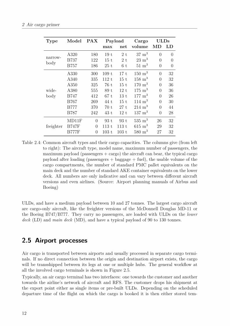
Table 2.4: Common aircraft types and their cargo capacities. The columns give (from leftto right): The aircraft type, model name, maximum number of passengers, themaximum payload (passengers + cargo) the aircraft can bear, the typical cargopayload after loading (passengers + baggage + fuel), the usable volume of thecargo compartments, the number of standard PMC pallet equivalents on themain deck and the number of standard AKE container equivalents on the lowerdeck. All numbers are only indicative and can vary between different aircraftversions and even airlines. (Source: Airport planning manuals of Airbus andBoeing)
ULDs, and have a medium payload between 10 and 27 tonnes. The largest cargo aircraftare cargo-only aircraft, like the freighter versions of the McDonnell Douglas MD-11 orthe Boeing B747/B777. They carry no passengers, are loaded with ULDs on the lowerdeck (LD) and main deck (MD), and have a typical payload of 90 to 130 tonnes.
2.5 Airport processes
Air cargo is transported between airports and usually processed in separate cargo termi-nals. If no direct connection between the origin and destination airport exists, the cargowill be transshipped between its legs at one or multiple hubs. The general workflow atall the involved cargo terminals is shown in Figure 2.5.Typically, an air cargo terminal has two interfaces: one towards the customer and anothertowards the airline’s network of aircraft and RFS. The customer drops his shipment atthe export point either as single items or pre-built ULDs. Depending on the scheduleddeparture time of the flight on which the cargo is booked it is then either stored tem-
12

2.5 Airport processes
expo
rtim
port break-down
build-up
piece store uld store
loading
unloading
Figure 2.5: Typical material flow in an air cargo terminal (gray arcs represent items, blackarcs ULDs). Cargo is unloaded at the terminal from incoming flights or trucks,or it is dropped by the customer at the export interface. Inside the terminalthe cargo is broken down from ULDs into single items, stored, and build upinto ULDs. The cargo leaves the terminal to be loaded into an aircraft ortruck, or to be picked up by the customer at the import interface.
porarily or directly sent to the build-up process. During build-up the items are packedonto ULDs. The ULDs are weighed and then loaded into an aircraft or RFS truck.After unloading at the next station the ULDs are again stored as a whole or broken downinto their items. These can then be picked up by the customer through the import pointor continue their journey towards their final destination.In the following, we describe the two processes relevant for load planning, namely thebuild-up and aircraft loading. The corresponding unload and break-down processes aresimpler and do not require as much description.
Build-up process
The build-up process is the most time consuming physical step done in an air cargoterminal. Here the ULDs are packed with cargo. See Figure 2.6 for a sample view intothe terminal build-up area. The workers start with one or more empty ULDs and anassortment of items assigned to the same transport segment. They have to pack theitems onto the ULDs in a legal and safe way. Large or heavy items are placed by using afork lift. Smaller items are usually placed by hand.This task is challenging for several reasons: The majority of ULDs is built several hoursbefore the flight departs. Therefore, the items at the workstation are generally a subsetof the cargo that already arrived at the terminal for the considered flight. As this amountof cargo can be quite large, see the stated volumes in Table 2.4, it is hard to keep trackof and to combine the shipments such that all items fit onto the ULDs. Furthermore, theworkers have to make sure that the weight limit for each ULD is not exceeded and the
13

2 Air cargo primer
Figure 2.6: Build-up workstations in a cargo terminal. Source: Lufthansa Cargo AG,Photographer: Werner Bartsch
given maximum contours for each ULD are respected. Single over-sized items might beplaced on a ULD with overhang and another ULD, which then has to be placed on anadjacent position in the aircraft, needs to leave some free space at the adverse position.The items have to be packed in a stable way, i.e., no tipping, slipping, or breaking becauseof too much top load is acceptable. This load stability is also required during takeoff,flight, and landing, when the aircraft is tilting or exposed to accelerating forces. Tosecure the items on pallet ULDs the workers use nets and straps. Furthermore, dunnagematerials like wooden boards or empty wooden pallets are used to distribute point loadsacross larger surfaces, to lock items into position, or to provide an even loading surfacefor further items.In addition, there is a constant pressure of time. Each aircraft has a scheduled departuretime and will rarely wait for a single missing ULD. Therefore, the decisions once madeduring build-up should not be revised too often.
Aircraft loading
The final physical step of the loading process is to load the built ULDs into the air-craft. The containers and pallets are loaded into special ULD compartments equippedwith rollers and latches on the floor, see Figure 2.7. Most aircraft have two separatecompartments on the lower deck, one in front of and another behind the center wing box,see Figure 2.8. Cargo aircraft also have a main deck compartment spanning along thefuselage. Most compartments only have a single door for the ULDs to enter and leave.Accordingly, loading is often a first-in-last-out (FILO) process. This is especially impor-tant for cargo aircraft as they frequently fly on multi-leg flights, i.e., they are not fullyunloaded at each airport and some ULDs will continue their journey on the same aircraft.Main deck compartments often have two separate lanes. Nevertheless, lateral movementsand rotations of ULDs can only be made near the door, where rotatable rollers are installedon the floor. Lower deck compartments usually have a single full width lane that can be
14

2.5 Airport processes
Figure 2.7: Aircraft loading: Empty main deck of a cargo aircraft with rollers and latcheson the floor (left). Loading of packed ULDs into the aircraft (right). Source:Lufthansa Cargo AG, Photographer: Jannah Baldus (right)
split to accommodate two half-width contoured containers. Each compartment is dividedinto distinct loading positions. An example of the loading positions of an MD11F is givenin Figure 2.8.In most cases, there is a standard configuration for each compartment, i.e., a valid assign-ment of ULD types to loading positions that maximizes the space utilization. Dependingon the installed floor latches other configurations might be possible. A typical change isto replace two standard ULDs by one large ULD to accommodate larger items. Otherreasons to deviate from the standard configuration might be a shortage of a certain ULDtype at the origin or destination airport, or to reduce the number of handling operations.To keep things simple, airlines therefore prefer a certain configuration and deviate fromit only if it is necessary.One important aspect of aircraft loading is called weight and balance (WAB). As shownin Table 2.4, the total payload an aircraft can carry is limited. Furthermore, the aircraftstructure has certain stress limits. There is a maximum weight for each loading positionand there also exist weight limits for various subsets of loading positions that are effectivelysmaller than the sum of their individual weight limits. Typically, there are limits foradjacent positions or positions above each other in the main and lower deck.Besides the weight limits there is a balance restriction. As each laden ULD has itsindividual weight and most ULDs could be placed at different loading positions in theaircraft, the loading assignment influences the aircraft’s center of gravity (CG). The CGalways has to stay within an allowed range, which depends on the aircraft type, to remainmaneuverable. If the aircraft is too nose-heavy, the front gear would not lift for takeoff.Or, if it is too tail-heavy, it might tip over on the ground. The lateral balance must alsobe respected but is usually less important as the lever is rather small compared to thelongitudinal balance. Additionally, the pilots are able to pump fuel between the left andright wing tanks to distribute the load evenly during flight. Besides the aircraft’s hardCG limits, there is an optimal CG individual to the aircraft at which it consumes theleast fuel. On most modern large commercial aircraft the optimal CG is close to the afthard CG limit. To get an impression of the CG impact on fuel consumption, Mongeau
15

2 Air cargo primer
AL
AR
BL
BR
CL
CR
DL
DR
EL
ER
FL
FR
GL
GR
HL
HR
JL
JR
KL
KR
LL
LR
ML
MR
P R
11P 12P 13P 21P 22P 23P 31P 32P 33P 41P
forward compartment aft compartment
Figure 2.8: Layout of the loading positions of an MD11F freighter aircraft (top: maindeck, bottom: lower deck). Doors are marked as thick lines along the fuselage.Standard loading positions are marked in gray. Alternative loading positionsfor larger ULDs (e.g., CR+DR or GR+GL) and smaller ULDs (e.g., 11L/R)are marked as dashed lines.
and Bes (2003) report that a CG shift of 75 cm on an Airbus A340 might lead to 4 tonnesof wasted fuel per 10,000 km flown.
2.6 SummaryIn this chapter, we provided a short introduction into the air cargo business and thecomponents one needs to understand the loading problems faced by cargo carriers.We started with pointing out the differences between the passenger and air cargo business,introduced the typical cargo characteristics, the container types (ULDs) into which thecargo is packed, as well as the types of aircraft used.After that, we introduced the outbound cargo handling processes, namely the build-upand aircraft loading. In the next chapter we define the general load planning problem inmore detail and the steps the carriers have to undertake before a cargo flight can start.
16

3 Air cargo load planning
In the last chapter, we introduced the two main physical processes conducted before acargo flight: the ULD build-up and aircraft loading. In this chapter, we look at theplanning tasks that go along with these physical actions.Our contribution here is twofold. First, we describe the full operational load planningproblem as faced by airlines that transport cargo. Only separate parts of it have yetbeen studied in the literature. Second, we discuss the challenges of current manual plan-ning approaches, which will lead us to our computerized planning approach proposed inChapter 9.In the following, we introduce the decisions made during load planning in Section 3.1 aswell as the airline’s stakeholders and their respective objectives in Section 3.2. We discussthe current state of the planning practice in Section 3.3 and identify current challengesin Section 3.4.
3.1 Planning tasks
In the daily practice of ULD build-up and aircraft loading at our industrial partner andfrom the present literature (Mongeau and Bes (2003), Rong and Grunow (2009), Paquayet al. (2016), Lurkin and Schyns (2015)) we identify four types of decisions to make:
1. What ULDs should be built?2. When should the ULDs be built?3. How to pack items on the ULDs?4. Where to load the ULDs inside the aircraft?
The parameters and constraints to make these decisions properly are quite extensive.Therefore, we split the general load planning into four subproblems. Each tackles onetype of decision:
1. Aircraft Configuration Problem (ACP):Select the types and number of the ULDs to be built for a flight.
2. Build-up Scheduling Problem (BSP):Decide at what time and workstation each ULD is built.
3. Air Cargo Palletization Problem (APP):Decide the assignment of items to and their placement inside the ULDs.
4. Weight and Balance Problem (WBP):Decide the loading positions of the ULDs inside the aircraft.
We denote the union of these four subproblems as the Air Cargo Load Planning Prob-lem (ACLPP). Parts of these subproblems and their constraints have already been studied

3 Air cargo load planning
sales
maximizeload
maximizerevenue
groundhandling even
workload
minimizeeffort
aircraftoperations
minimize fuelconsumption
minimize ULDoperations
Figure 3.1: Load planning stakeholders and their main objectives
separately in the literature. To our knowledge, there is no published work yet that de-scribes the planning problems and related processes in the practically required level ofdetail. We introduce the ACLPP by its four subproblems in detail in the upcomingChapters 4 to 7.
3.2 Stakeholders and objectives
We identify three stakeholders whose objectives need to be considered during load plan-ning. These are the departments of sales, handling, and aircraft operations. An overviewof their main objectives is given in Figure 3.1.The sales department offers the cargo capacity of all flights to the customers. Its mainobjective is to maximize the revenue of each flight. Besides maximizing the space uti-lization, the desired load plans should therefore also allow to transport as much specialcargo as possible. Outsized items, dangerous goods, or living animals might have specialloading requirements but usually provide much higher yields than standard cargo.The handling department executes all cargo operations inside the cargo terminal. Theyreceive (deliver) cargo from (to) the customers at the ramp, store it in and retrieve itfrom the warehouse, and perform the ULD build-up and break-down. As the build-upand aircraft loading processes have tight deadlines, the primary handling objective is tominimize loading effort and keep things simple. Furthermore, the workload should beevenly distributed throughout the day to reduce peak demands for workers and worksta-tions.The aircraft operations department prepares the aircraft for each flight. In particular, itplans how the aircraft is loaded and fueled. Besides loading complete set of built ULDs, ithas two main objectives. First, to reduce the amount of required fuel by distributing theload inside the aircraft in the best possible way. Second, the ULDs should be arranged ina way that only a small number of reloading operations are necessary at each stop-over
18

3.3 Traditional planning practice
Sales Handling OperationsAircraft Configuration Problem (ACP)
maximize load/revenues + − −minimize handling effort − + +
Build-up Scheduling Problem (BSP)even workload − + ◦late build-ups + − −
Air Cargo Palletization Problem (APP)maximize load/revenues + − −minimize handling effort − + ◦
Weight and Balance Problem (WBP)minimize fuel consumption − ◦ +minimize handling operations ◦ + +
Table 3.1: Overview of subproblem objectives and how they align with the goals of thestakeholders, i.e., sales, ground handling, and flight operations. We mark threelevels: conformity (+), conflict of interest (−), and no influence (◦).
airport. This reduces the turnaround time as well as the wear and tear of the aircraft,and results in less risk to damage the cargo.In Table 3.1 we give an overview where the stakeholders’ goals echo in the objectives ofthe defined subproblems and how they affect the goals of the other stakeholders. Forexample, the minimization of effort during palletization might have a negative impact onthe sales goals (−) as it reduces the aircraft utilization. It has a positive impact on thehandling goals (+) as it reduces the number of handling operations. The goals of flightoperations are not influenced (◦) by the handling effortFrom our experience, there is no clear hierarchy of objectives. What is most importantstrongly depends on the overall situation. On a highly booked flight load maximizationseems to be the top priority. However, if the flight departs during a rush hour, it mightalso be important to keep the handling effort low to be able to meet all deadlines. Finally,weight and balance might become a driving factor on long-haul flights that operate at theaircraft limits.
3.3 Traditional planning practice
In this section, we describe the traditional planning practice at our industrial partner. Werefrain from a more detailed description for confidentiality. The ACLPP is an operationalproblem and needs to be solved roughly throughout the last 24 hours before each flight.Flights departing at around the same time compete for the same build-up resources.Therefore, their planning problems are interwoven. When the load planning begins, mostparameters like the booked cargo and the workforce in the terminal are mostly fixed.
19

3 Air cargo load planning
Corresponding to the four subproblems introduced in Section 3.1, the planning process issplit into four stages each performed by appropriately trained workers.In the first stage, denoted as load planning, the planners select the ULD types and theirrespective number to built for each destination airport of the flight. They do this basedon the booked cargo weight and volume for each destination, the aircraft specifications,internal regulations, as well as their personal experience. Furthermore, they add someextra ULDs that should be filled with low priority cargo. These ULDs will be built andsent to the aircraft but will only be loaded into it if an originally planned ULD is notloadable. This might happen if a ULD arrives too late or is not properly packed and thusrejected by the ramp agent at the aircraft. Usually, items are not assigned to specificULDs yet, but the planners might already suggest a certain ULD or ULD type for specialcargo. The list of ULDs to build and the suggested assignments are forwarded to the nextstage.In the second stage, denoted as build-up planning, the planners decide about the scheduleof build-ups for all outgoing flights. They trigger the build-up of groups of ULDs andassign an available workstation to them. Only nonstandard ULDs are scheduled on anindividual basis. The basic weekly workstation schedule, defining which flights are builtwhen and where, is predetermined usually for a full six-month flight plan. Accordingly,the planners mostly supervise the task queue at each workstation and manually inter-vene when disruptions occur. Furthermore, the planners make sure that enough cargo isavailable at the workstations. They release batches of shipments from the warehouse andsend them to the workstations. Except for the suggested assignments from the first stage,still no individual items are picked at this stage. Thus, the result of the second stage areworkstations set up with empty ULDs and an assortment of cargo.In the third stage, denoted as palletization, the workers pack the cargo into the ULDs.They decide which item is placed onto which ULD and where. The goal is generally to putas much cargo as possible onto the ULDs. On overbooked flights, as few items as possibleshould be left behind at the cargo terminal. Even if a flight is not fully booked, densepacking is a goal as the remaining space can be filled with shipments booked on laterflights to the same destination that already arrived at the terminal. The workers usuallydecide ad-hoc about the item placement based on their experience and the availablecargo within visual range. To get an impression of what is stackable and what is not,the workers frequently touch and feel the items. Usually, they start with large, heavy, orother critical items and finish with small undemanding cargo. Furthermore, they mightuse dunnage material to provide an even base for further items or to protect and secureitems. During the entire build-up process, the workers have to ensure the load safety andloading restrictions, like those stemming from dangerous goods regulations (DGR) definedby IATA (2016). The workers are responsible for a safe and legal build-up. At the verylast, the workers close the ULDs. ULD pallets are covered with a net and lashed withstraps. Inside ULD containers the items are locked into position by straps if necessarybefore the container’s doors are closed. The finished ULDs are sent to a weigh stationand stored until they are sent out to the aircraft.In the fourth stage, denoted as weight and balance, the planners assign the assembledULDs to loading positions inside the aircraft. They usually apply a greedy strategystarting to place heavy ULDs at the center of the aircraft and then moving outwards.
20

3.4 Challenges of current practice
After all ULDs have been placed, the planner might apply local modifications changingthe aircraft’s center of gravity to reduce its fuel consumption. During this manual processthe planner is supported by tools that calculate the aircraft’s performance indicators.Tools that check the feasibility of a load plan are usually already provided by the aircraftmanufacturer. The final plan is delivered to the aircraft, where the ramp agent loads theULDs accordingly. He can still make final adjustments if a ULD cannot be loaded andhas to be replaced by one of the available low priority ULDs.
3.4 Challenges of current practice
The procedures described in the last section provide several challenges. Most obvious,many decisions are made manually by the planners although there is a constant pressureof time and the problems at hand are demanding. One result of this situation is, thatthe planners often stop at the first feasible solution they find. Thus, they only solve thesatisfiability part of what is an optimization problem. Furthermore, as safety is a majorissue in the airline industry, the planner’s decisions are repeatedly checked in the laterstages to make sure no constraint is violated. Altogether, a lot of manpower is involvedin a process that seems to be automatable.We attribute the current lack of automation to two reasons. First, the data needed forautomated planning are just becoming gradually available and data quality still needs toimprove. In the past, booking data only contained the total shipment weight and volume,not individual items. Today, the shipper can provide item dimensions, but sometimesthese might not be defined at the time of booking or they change afterwards. To improvedata quality, cargo airlines start using item scanners at their terminals to update theshipment data as soon as they get hold of it. Throughout this work, we therefore assumethat these data challenges can be solved in the future.The second reason is the lack of suitable planning models. Only parts of the processlike the weight and balance stage have recently been subject to research, see Lurkin andSchyns (2015). The palletization stage is at its core a classical optimization problem,the multidimensional Knapsack Problem. First articles are examining it in an air cargocontext, see Paquay et al. (2016), but the full set of its constraints has not been studiedin the literature in its entirety. For the first two stages, only loosely related articles canbe found.Besides the automation issues, there are other challenges present at the interfaces of theplanning stages. The stages are processed strictly sequential (see Figure 3.2) and eachstage has its own constraints and objective. In practice, this approach leads to only localoptimization or worse, to infeasible problem states in later stages. Infeasibility typicallyleads to offloads, i.e., some of the shipments have to be rebooked on another flight causinglost revenue or even penalties. In the following, we describe a few situations that can befound in practice if the stages are not properly coordinated.First, the build-up planners often have to schedule a ULD build-up several hours beforethe flight due to a limited workstation capacity later. But, at the time of build-up noshipments to pack might be physically available. Thus, the ULD cannot be built or isdelayed and might cause a shortage of handling capacity later on.
21

3 Air cargo load planning
Aircraft configuration
Build-up scheduling
Palletization
Weight and balance
number andtypes of ULDs
ULD type andavailable items
loaded andweighed ULDs
Figure 3.2: Sequential workflow of load planning in practice
Another issue in practice is that the palletization workers only see the shipments thatare present at their workstation. They continuously pack the items onto the ULDs whilefurther shipments are released by the build-up planners and arrive at the workstation. Ifa large item arrives late, the worker might not find a suitable empty space for it althoughthe total volume and weight capacity of the ULD is not fully utilized. So, the large itemmust be rebooked.In the weight and balance stage, the weights of all the ULDs are already fixed. They area result of the palletization. As the palletization workers try to fully utilize the ULDs,they typically build some heavy ULDs first and lighter ones later. This might result in anunfavorable weight distribution between the ULDs. So, the weight and balance plannermight only find suboptimal solutions that consume more fuel or need more ULD reloadingoperations at the stop-over airports than necessary. Both results in higher cost.
3.5 SummaryIn this chapter, we provided an overview of the load planning problems faced by cargoairlines. We introduced the three stakeholders: sales, handling, and aircraft operations,and their objectives: maximizing revenue, minimizing physical handling effort, and min-imizing operational cost of the flight. Furthermore, we discussed the challenges of thecurrently implemented planning approaches. The identified challenges motivate the workof this thesis and lead to our solution approaches presented in Chapters 9 and 11.Prior to that we define the identified subproblems one by one in the next four chapters,discuss the related literature and present a comprehensive mathematical formulation.
22
4 Aircraft configuration
Aircraft configuration
Build-up scheduling
Palletization
Weight and balance
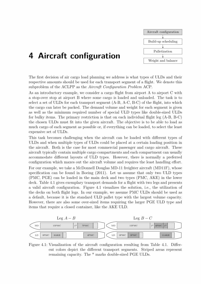
The first decision of air cargo load planning we address is what types of ULDs and theirrespective amounts should be used for each transport segment of a flight. We denote thissubproblem of the ACLPP as the Aircraft Configuration Problem ACP.As an introductory example, we consider a cargo flight from airport A to airport C witha stop-over stop at airport B where some cargo is loaded and unloaded. The task is toselect a set of ULDs for each transport segment (A-B, A-C, B-C) of the flight, into whichthe cargo can later be packed. The demand volume and weight for each segment is givenas well as the minimum required number of special ULD types like double-sized ULDsfor bulky items. The primary restriction is that on each individual flight leg (A-B, B-C)the chosen ULDs must fit into the given aircraft. The objective is to be able to load asmuch cargo of each segment as possible or, if everything can be loaded, to select the leastexpensive set of ULDs.This task becomes challenging when the aircraft can be loaded with different types ofULDs and when multiple types of ULDs could be placed at a certain loading position inthe aircraft. Both is the case for most commercial passenger and cargo aircraft. Theseaircraft typically contain multiple cargo compartments and each compartment can usuallyaccommodate different layouts of ULD types. However, there is normally a preferredconfiguration which maxes out the aircraft volume and requires the least handling effort.For our example, we take a McDonnell Douglas MD-11 freighter aircraft (MD11F), whosespecification can be found in Boeing (2011). Let us assume that only two ULD types(PMC, PGE) can be loaded in the main deck and two types (PMC, AKE) in the lowerdeck. Table 4.1 gives exemplary transport demands for a flight with two legs and presentsa valid aircraft configuration. Figure 4.1 visualizes the solution, i.e., the utilization ofthe decks on both flight legs. In our example, we assume PMC ULDs should be used asa default, because it is the standard ULD pallet type with the largest volume capacity.However, there are also some over-sized items requiring the larger PGE ULD type anditems that require a closed container, like the AKE ULD.
Leg A−BMD 15PMC 1* 7PMC
LD 3PMC 8AKE 4PMC
Leg B − CMD 15PMC 1* 4PMC 1*
LD 3PMC 3PMC 11AKE
Figure 4.1: Visualization of the aircraft configuration resulting from Table 4.1. Differ-ent colors depict the different transport segments. Striped areas representremaining capacity. The * marks double-sized PGE ULDs.

4 Aircraft configuration
ULD type MD LD fwd LD aftPMC PGE PMC AKE PMC AKE
max volume (m3) 19 39 15 4 19 4max weight (t) 6.8 11.3 5.1 1.5 5.1 1.5#ULDs per segmentA→ C (380 m3, 66 t) 16 1 3 0 0 0A→ B (240 m3, 42 t) 8 0 0 8 4 0B → C (210 m3, 37 t) 4 1 3 0 0 14#ULDs on legA−B 24 1 3 8 4 0B − C 20 2 6 0 0 14
Table 4.1: Example aircraft configuration for a flight with two legs. The “#ULDs persegment” rows give the number of selected ULDs per compartment. The totaldemand (volume, weight) is given inside the parentheses. The last two rowsgive the total number of ULDs flown on each leg.
From a theoretical perspective the ACP combines two nested packing problems. The innerproblem is that enough ULDs must be reserved for each segment of the flight to coverthe cargo demand. To fully solve it, one would also need to solve the three-dimensionalpacking problem that is the subject of the palletization stage presented in Chapter 6. Fromthe operational practice of our industrial partner we learned that this level of detail is notnecessary to find suitable aircraft configurations. Instead, a simplified one-dimensionalconsideration, with respect to cargo volume and weight, seems sufficient in practice.The outer problem is that on each leg the ULDs of all segments using this leg must fit intothe aircraft. This problem must be solved in parallel for all legs of a flight as the set ofloaded ULDs might change at each stop-over airport. We assume that each compartment’scapacity can be described by a set of linear restrictions of the present ULD types.In the following, we give a few examples of typical compartment combination restrictions.In the simplest form the compartment has a number of capacity units and each ULD typeconsumes a certain amount of them. On our sample aircraft the main deck has 26 units.Here, a PMC ULD consumes one unit and a PGE ULD two units. So, the restriction canbe stated as 2|PGE| + |PMC| ≤ 26. Depending on the valid ULD combinations morethan one linear restriction might be needed to express the configuration space. Let usassume in our example that we can choose one of the configurations shown in Figure 4.2for the lower deck aft compartment (not all ULDs must be present). Note that theconfiguration space is not convex with respect to the loadable number of ULDs per type.Then, besides our general restrictions, |AKE| ≤ 14 and |PMC| ≤ 4, either |AKE| ≤ 4and 16− |AKE| ≤ 4|PMC| must hold or 14− |AKE| ≤ 4|PMC|.In the next section, we discuss the present literature related to the ACP followed by itsmathematical formulation in Section 4.2.
24

4.1 Related literature
4PM
C
3PM
C,4
AKE
2PM
C,6
AKE
1PM
C,1
0AKE
14AKE
Figure 4.2: Exemplary ULD configurations inside a compartment. Starting on the leftwith 4 PMC pallets and replacing them by AKE containers until the com-partment is filled with 14 AKEs.
4.1 Related literature
To the best of our knowledge there is no work regarding the ACP as introduced in thelast section. However, aspects of the ACP have already been studied in the literature.Yan et al. (2006) present a model to decide for a whole flight network which cargo streamsshould be loaded and combined into which ULD type and compartment. Their objectiveis to minimize the total ULD handling cost. The main idea is to combine cargo for thesame final destinations early such that these single-destination ULDs must not be handledagain. The model was formulated as a non-linear mixed integer program and evaluatedon the Asia Pacific network of FedEx using IBM’s CPLEX solver. All instances containedonly two ULD types, one for main deck positions and another for lower deck positions.That means only a single aircraft configuration is considered, since ULD types cannot beexchanged for another. Furthermore, the model applies to single-leg flights only.Besides, aircraft configuration restrictions are also considered in some papers dealing withaircraft weight and balance. Here, the cargo is already packed onto ULDs of differenttypes and the ULDs have to be assigned to loading positions in the aircraft. If multipleULD types have to be loaded and more ULDs are present than loading positions exist,then these models might also decide about the configuration. Mongeau and Bes (2003)present a problem with different ULD types and an elaborate description of the constraintslimiting the combinations of ULD types for each compartment of an Airbus A340. Tomodel the constraints, they introduce multiple linear combinations of the amounts perULD type for each compartment and put a limit on these. Limbourg et al. (2012) presenta model assigning ULDs to loading positions in the aircraft. They implicitly decide aboutthe configuration by restricting the usage of partially overlapping positions. The samemodel is extended by Lurkin and Schyns (2015) for multi-leg flights.
4.2 The Aircraft Configuration Model
In this section, we define a mathematical model of the ACP, which we denote as theAircraft Configuration Model (ACM) in the following. The goal of the ACP is to find a
25

4 Aircraft configuration
set of ULDs for each transport segment of a flight that minimizes the total cost, i.e., thesum of the cost of all selected ULDs plus the penalties for offloaded cargo.We start by defining the input parameters and decision variables followed by the problem’sconstraints and objective. At last, we present a short overview of the model.
4.2.1 Input parameters
The ACM considers four sets of entities. Let L denote the set of flight legs, K the set oftransport segments, V the set of ULD types, and F the set of sets of ULD combinationrestrictions of the aircraft. We use the respective lower case indices to represent singleentities: f ∈ G for each G ∈ F , k ∈ K, l ∈ L, v ∈ V .
Flight parameters• onk ⊆ L: set of flight legs of transport segment k• startl ⊆ K: set of transport segments starting with flight leg l
Aircraft parameters• limitf ∈ R: total ULD limit in combination restriction f• mf,v ∈ R: factor of ULD type v in combination restriction f
ULD parameters• availl,v ∈ N: available units of ULD type v at departure airport of leg l• capvolv ∈ R≥0: volume capacity per ULD of type v• capwgtv ∈ R≥0: weight capacity per ULD of type v• costv ∈ R: handling cost per ULD of type v (preparation, loading, unloading)
Demand parameters• demvol
k ∈ R≥0: total volume of shipments on segment k• demwgt
k ∈ R≥0: total weight of shipments on segment k• mink,v ∈ N: minimum required number of ULDs of type v on segment k• offloadvolk ∈ R≥0: penalty for offloaded shipment volume on segment k• offloadwgtk ∈ R≥0: penalty for offloaded shipment weight on segment k
4.2.2 Decision variables
The primary decision made by the model is the number of selected ULDs for each transportsegment. If not all cargo is loaded, we also need to decide the offloaded weight and volume.• xk,v ∈ N: number of selected ULDs on segment k of type v• yvolk ∈ R≥0: offloaded volume on segment k• ywgtk ∈ R≥0: offloaded weight on segment k
26

4.2 The Aircraft Configuration Model
4.2.3 Constraints
In the following, we introduce the constraints that define a valid aircraft configuration. Wenote that a solution to this subproblem alone does not guarantee a feasible ULD loadingsince only a simplification of the three-dimensional packing constraints is considered.Further constraints to guarantee the feasibility will be added in Chapter 6.
Capacity reservation For each transport segment k the capacity of the selected ULDsmust be large enough to accommodate the transported shipments by volume and weight.The transported amount is the difference of the demand and the offloaded shipments:∑
v∈Vxk,vcapwgtv ≥ demwgt
k − ywgtk k ∈ K (4.1)∑v∈V
xk,vcapvolv ≥ demvolk − yvolk k ∈ K (4.2)
Combination restrictions On each flight leg l the ULDs of all present segments mustadd up to a valid aircraft configuration. We model the valid configurations implicitly bythe allowed ULD type combinations. The given restrictions F are organized in groups.Similar to a logic formula given in conjunctive normal form, for all groups G ∈ F at leastone restriction f ∈ G must hold. Thereby, alternative non-convex combinations can bemodeled. Each restriction f represents a valid linear combination of ULDs, which canbe loaded into the aircraft. Each ULD type v is weighted by a parameter mf,v and thesum is limited by parameter limitf . Furthermore, we introduce an auxiliary variable bl,findicating if restriction f is fulfilled on leg l and make sure that at least one bl,f equals 1for each group:∑
k∈K:l∈onk
∑v∈V
mf,vxk,v ≤ limitf + (1− bl,f )M l ∈ L;G ∈ F ; f ∈ G (4.3)∑f∈G
bl,f ≥ 1 l ∈ L;G ∈ F (4.4)
Required ULD types For each segment some ULDs of certain types might be requiredto load special cargo. In practice this requirement arises when very large, heavy or fragileitems are among the shipments. Large items might require a larger ULD type, heavyitems a ULD type with a reinforced floor area, or fragile items should only be loaded intoa closed ULD container. Another source of required ULD types is that in practice cargomight already be loaded on a ULD and this ULD should be used for further build-up.All these requirements can be precalculated and the number of the respective ULD typeslimited accordingly:
mink,v ≤ xk,v k ∈ K; v ∈ V (4.5)
Airport ULD type limits The airline might not have an unlimited supply of all ULDtypes at all departure airports. Therefore, we need to respect the availability limits for
27

4 Aircraft configuration
ULDs that should be build-up at an airport. This restriction applies only to transportsegments whose first leg starts at the given airport:∑
k∈K:k∈startl
xk,v ≤ availl,v l ∈ L; v ∈ V (4.6)
4.2.4 Objective
While satisfying all the given constraints, we want to load as much cargo as possibleand choose the least expensive set of ULDs for it. The parameter costv for ULD type vrepresents the fixed handling cost for build-up and break-down, the transport to and fromthe aircraft, the loading into and out of the aircraft, as well as the wear and tear of theULD itself. The penalty for offloaded volume offloadvolk and weight offloadwgtk comprisesthe lost revenues and the impact on customer satisfaction for shipments on segmentk. The penalties can only be estimated, but reasonable values can be chosen basedon the segment’s travel distance or the effective delay of offloaded shipments based on thefrequency at which the airline serves this route.Thus, the objective is to minimize the total cost:
minimize∑k∈K
(ywgtk offloadwgtk + yvolk offloadvolk +
∑v∈V
xk,vcostv)
(4.7)
Note that this formulation can tackle both bin packing and knapsack style problems. Ifthere is little demand the number of ULDs is reduced. If the demand exceeds the aircraftcapacity the least important cargo is offloaded.
4.2.5 Model overview
After introducing all components of the ACM in the last sections, we now give a consoli-dated view of the full model:
minimize∑k∈K
(∑v∈V
xk,vcostv + ywgtk offloadwgtk + yvolk offloadvolk
)(4.8)
subject to
demwgtk ≤
∑v∈V
xk,vcapwgtv + ywgtk k ∈ K (4.9)
demvolk ≤
∑v∈V
xk,vcapvolv + yvolk k ∈ K (4.10)
limitf ≥∑
k∈K:l∈onk
∑v∈V
mf,vxk,v + (bl,f − 1)M l ∈ L; f ∈ F (4.11)
1 ≤∑f∈G
bl,f l ∈ L;G ∈ F (4.12)
mink,v ≤ xk,v k ∈ K; v ∈ V (4.13)
28

4.3 Summary
availl,v ≥∑
k∈K:k∈startl
xk,v l ∈ L; v ∈ V (4.14)
xk,v ∈ N k ∈ K; v ∈ V (4.15)ywgtk , yvolk ∈ R≥0 k ∈ K (4.16)bl,f ∈ {0, 1} l ∈ L;G ∈ F (4.17)
The objective, given in Equation (4.8), is to minimize the total cost from the used ULDsand offloaded cargo. Equation (9.3) and (9.4) model the capacity reservation, Equa-tions (9.5) and (9.6) the ULD combination restrictions, Equation (9.7) the minimumrequired ULDs, and Equation (9.8) the airport ULD type limit.
4.3 SummaryIn this chapter, we introduced the Aircraft Configuration Problem (ACP) in detail, whichis to decide what ULD types and amounts should be selected for each transport segment.Furthermore, we analyzed the related literature and presented a formal model, denotedas Aircraft Configuration Model (ACM), of its features.The literature containing aspects of aircraft configuration from a load planning perspec-tive is very scarce. In most works on aircraft loading, only a single configuration isconsidered or only one ULD type can be placed on each loading position. In both casesthe problem becomes much easier, but significant parts of the configuration space of atypical cargo aircraft are not covered. Aspects of aircraft configuration have also beenpresent in papers dealing with weight and balance. Here, the ULDs are already built andweighed. Therefore, only one part of the problem remains, which is to combine differentULD types into the compartments.The presented model contains two nested packing problems. The inner is a vector packingproblem, with respect to weight and volume, that assigns demand to ULDs. The outermatches the ULDs to aircraft compartments and fulfills aircraft specific loading restric-tions. The overall objective is to minimize the costs from offloaded demand and usedULDs.
29


5 Build-up scheduling
Aircraft configuration
Build-up scheduling
Palletization
Weight and balance
The second step of air cargo load planning we discuss is to decide when to actually packthe cargo into ULDs. We denote this subproblem of the ACLPP as the BSP.Throughout the day an air cargo terminal handles many outgoing flights. All theseflights compete for the same scarce build-up resources, namely workstations and workers.Therefore, some planning is needed to build-up all ULDs on time. As speed is a majorsales argument for air cargo, shipment itineraries often only have a short transfer timebetween their incoming and outgoing flight. So, part of the cargo only becomes physicallyavailable for the build-up shortly before its outgoing flight. Therefore, we need to takethe cargo arrivals into account to decide when to pack cargo into ULDs.As shown in Figure 2.5, cargo arrives at the terminal in two ways. Either it is dropped atthe export point by the shipper or his forwarder, or it arrives on an inbound flight. Onboth ways the arrival times are usually predictable. If a time window management systemis used at the export point, a rough handover time is known. Similarly, the arrival timeof an inbound flight is known and even unlikely to change during the last hours when itis already on its way.On the other end, the built ULDs need to be transported to the aircraft on time. Atmajor airports, where the distance between terminal and aircraft can be quite long, thisready-for-delivery due date might be an hour or more ahead of departure. Within thewindow of item arrivals and ULD due dates the ULDs have to be built.For economic reasons, there is usually only a limited capacity of workstations and workersavailable at the terminal. Both should be used evenly over time to limit stress and provideflexibility. During outbound rush hours the build-up capacity is usually too low to handleall outgoing ULDs. For example Figure 5.1 sketches the total outbound capacity of theLufthansa Cargo Hub in Frankfurt during one day. There is a peak at noon where morethan 15 percent of the day’s capacity departs within one hour. Under the assumption ofa constant build-up rate, the workload of the peak hour alone takes nearly four hours.Accordingly, some ULDs have to be built earlier than their due date. But, packing ULDsbefore all shipments arrived leaves fewer options in combining items. In a previous studywe have shown that the best possible bin utilization reduces if a part of the items arrivesafter the first bins are built (Brandt et al., 2014). The study considered one-dimensionalpacking only. We measured a loss of utilization if less than 70 percent of the remainingcargo volume was available on average when a bin is built. For each 10 percent lessavailable cargo the best possible utilization reduced by around 1 percent. To give anexample, we would expect a loss of 3 percent in utilization if on average only 40 percentof the cargo is available at each build-up. We note that the study only considered one-dimensional packing. The effects for three-dimensional packing will presumably be larger.
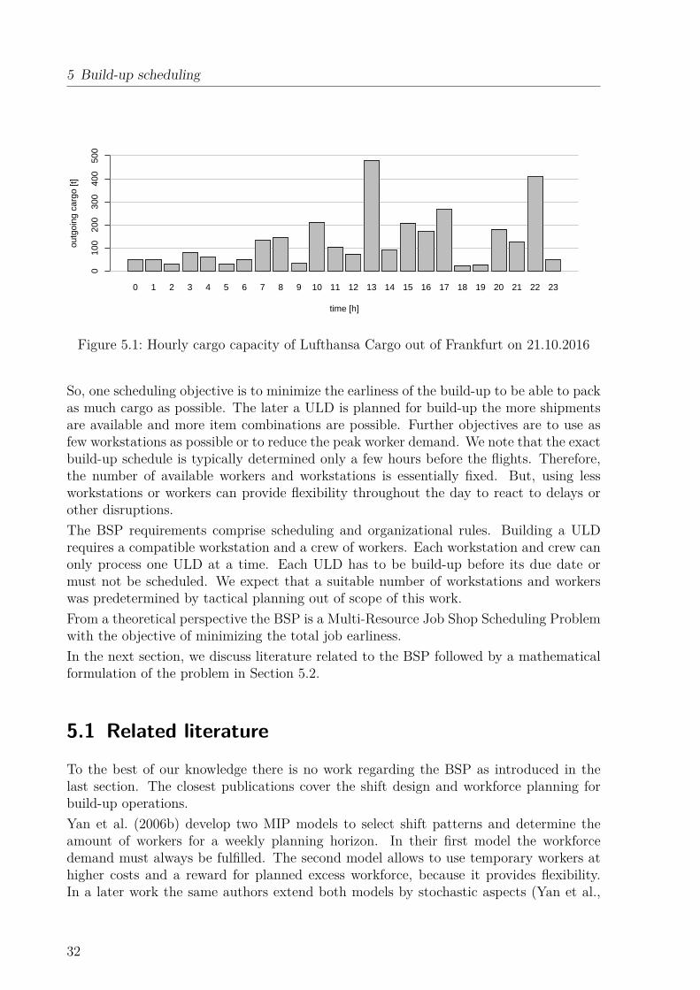
5 Build-up scheduling
0 1 2 3 4 5 6 7 8 9 10 11 12 13 14 15 16 17 18 19 20 21 22 23
time [h]
outg
oing
car
go [t
]
010
020
030
040
050
0
Figure 5.1: Hourly cargo capacity of Lufthansa Cargo out of Frankfurt on 21.10.2016
So, one scheduling objective is to minimize the earliness of the build-up to be able to packas much cargo as possible. The later a ULD is planned for build-up the more shipmentsare available and more item combinations are possible. Further objectives are to use asfew workstations as possible or to reduce the peak worker demand. We note that the exactbuild-up schedule is typically determined only a few hours before the flights. Therefore,the number of available workers and workstations is essentially fixed. But, using lessworkstations or workers can provide flexibility throughout the day to react to delays orother disruptions.The BSP requirements comprise scheduling and organizational rules. Building a ULDrequires a compatible workstation and a crew of workers. Each workstation and crew canonly process one ULD at a time. Each ULD has to be build-up before its due date ormust not be scheduled. We expect that a suitable number of workstations and workerswas predetermined by tactical planning out of scope of this work.From a theoretical perspective the BSP is a Multi-Resource Job Shop Scheduling Problemwith the objective of minimizing the total job earliness.In the next section, we discuss literature related to the BSP followed by a mathematicalformulation of the problem in Section 5.2.
5.1 Related literature
To the best of our knowledge there is no work regarding the BSP as introduced in thelast section. The closest publications cover the shift design and workforce planning forbuild-up operations.Yan et al. (2006b) develop two MIP models to select shift patterns and determine theamount of workers for a weekly planning horizon. In their first model the workforcedemand must always be fulfilled. The second model allows to use temporary workers athigher costs and a reward for planned excess workforce, because it provides flexibility.In a later work the same authors extend both models by stochastic aspects (Yan et al.,
32

5.2 The Build-up Scheduling Model
2008a). Both previous works are also published as Yan et al. (2006a) and Yan et al.(2008b) with negligible changes.Nobert and Roy (1998) present a MIP model to select shift patterns and determine theamount of workers for a typical day. Their goal is to minimize the total shift cost. Thetotal handling demand is given as a matrix of cargo arrivals and their correspondingdepartures for each period. Rong and Grunow (2009) present a similar model but alsoschedule the amount of cargo of each individual flight in the break-down and build-up foreach period.Both models do not consider individual ULDs or workstations. Instead they only limitthe total handling capacity across all flights for each time slot. While this seems fine toestimate the total workforce demand, it is not sufficient to plan ULD build-ups. In ourcase both approaches might lead to undesired solutions where many ULDs are partiallybuilt in each period. In reality, this would lead to many started ULDs blocking theworkstations for several periods before they can be finished. Furthermore, both papersdo not aim at a particular early or late build-up.For further reading, we refer to a recent review of publications concerning air cargo ter-minal operations which is given by Feng et al. (2015).
5.2 The Build-up Scheduling ModelIn this section, we define a mathematical model of the BSP, which we denote as theBuild-up Scheduling Model (BSM) in the following. The goal of the model is to find anassignment of the planned ULDs to build-up periods, while respecting workstation andworker capacity restrictions and performing build-ups as late as possible. We expect thatsufficient workforce is available to handle the total cargo demand throughout the day.This can be ensured by applying the same model earlier during tactical planning with theexpected upper bound of demand. The basis for our model is the model given by Rongand Grunow (2009). Instead of scheduling a certain amount of demand in each period,we schedule the ULDs and their respective workload explicitly.We start by defining the problem parameters. In the following sections we introduce theproblem’s constraints and the objective. At last, we present a short overview of the model.
5.2.1 Input parameters
The BSM considers four sets of entities. Let K denote the set of transport segments forwhich ULDs have to be build, V the set of ULD types, and S the set of shifts of thebuild-up crews. Furthermore, let T denote the periods of the planning horizon. In thefollowing we use the respective lower case indices to represent single elements: k ∈ K,s ∈ S, t ∈ T , v ∈ V .
Segment parameters• availvolk,t ∈ R≥0: cargo volume of segment k arriving up to period t• demvol
k ∈ R≥0: total cargo volume on segment k
33

5 Build-up scheduling
• duek ∈ T : build-up due date of segment k• losscostk ∈ R≥0: expected cost if a unit of the volume on segment k cannot be loaded• splitk ∈ N: maximum number of ULDs to build simultaneously for segment k• uldk,v ∈ N: number of ULDs of type v to schedule for segment k
ULD parameters• durv ∈ N: number of periods to build a ULD of type v• capvolv ∈ R≥0: volume capacity per ULD of type v
Capacity parameters• costs ∈ R≥0: cost of one build-up crew in shift s• ends ∈ T : last period after shift s• maxs ∈ N: maximum available build-up crews in shift s• openv,t ∈ N: number of workstations that can handle ULD type v during period t• starts ∈ T : first period of shift s
5.2.2 Decision variables
The primary decision made by the model is the number of ULDs to start building at eachperiod. To calculate the objective value, we introduce further decision variables. Onepart of the objective is to load as much as possible. There are two reasons that mightprevent us from achieving this goal: First, if not all ULDs can be scheduled for build-up.Second, if a ULD is scheduled before enough cargo is available. We capture the effect ofeach reason in one variable. Furthermore, we decide about the number of build-up crewsto deploy during each shift.• startk,v,t ∈ N: number of ULDs of type v started to build at period t for segment k
(t ≤ duek − durv)• offloadk,v ∈ N: number of not scheduled ULDs of type v on segment k• deadk,t ∈ R≥0: lost volume capacity on segment k if ULDs are built before enough
cargo volume is available• crewss ∈ N: number of selected build-up crews in shift s
5.2.3 Constraints
In the following we define the constraints that define a feasible build-up schedule.
Schedule ULDs All requested ULDs have to be scheduled to a period before the duedate or marked as offloaded.∑
t∈T :t≤duek−durv
startk,v,t = uldk,v − offloadk,v k ∈ K; v ∈ V (5.1)
34
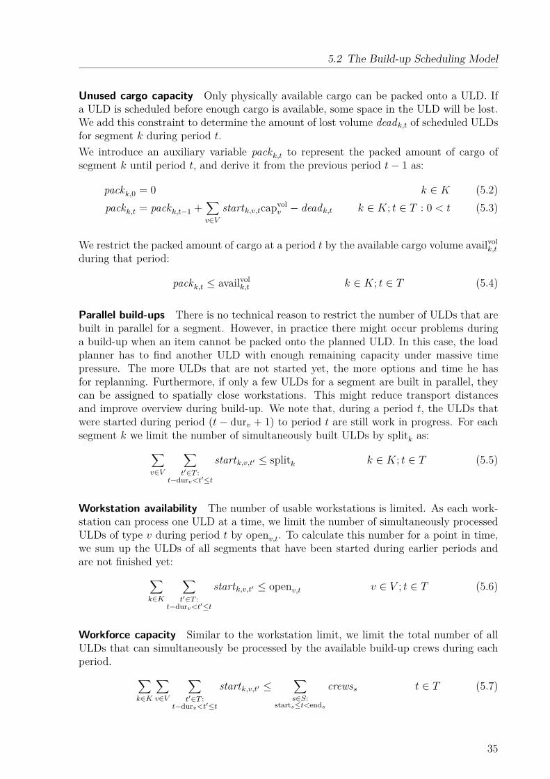
5.2 The Build-up Scheduling Model
Unused cargo capacity Only physically available cargo can be packed onto a ULD. Ifa ULD is scheduled before enough cargo is available, some space in the ULD will be lost.We add this constraint to determine the amount of lost volume deadk,t of scheduled ULDsfor segment k during period t.We introduce an auxiliary variable packk,t to represent the packed amount of cargo ofsegment k until period t, and derive it from the previous period t− 1 as:
packk,0 = 0 k ∈ K (5.2)packk,t = packk,t−1 +
∑v∈V
startk,v,tcapvolv − deadk,t k ∈ K; t ∈ T : 0 < t (5.3)
We restrict the packed amount of cargo at a period t by the available cargo volume availvolk,t
during that period:
packk,t ≤ availvolk,t k ∈ K; t ∈ T (5.4)
Parallel build-ups There is no technical reason to restrict the number of ULDs that arebuilt in parallel for a segment. However, in practice there might occur problems duringa build-up when an item cannot be packed onto the planned ULD. In this case, the loadplanner has to find another ULD with enough remaining capacity under massive timepressure. The more ULDs that are not started yet, the more options and time he hasfor replanning. Furthermore, if only a few ULDs for a segment are built in parallel, theycan be assigned to spatially close workstations. This might reduce transport distancesand improve overview during build-up. We note that, during a period t, the ULDs thatwere started during period (t− durv + 1) to period t are still work in progress. For eachsegment k we limit the number of simultaneously built ULDs by splitk as:∑
v∈V
∑t′∈T :
t−durv<t′≤t
startk,v,t′ ≤ splitk k ∈ K; t ∈ T (5.5)
Workstation availability The number of usable workstations is limited. As each work-station can process one ULD at a time, we limit the number of simultaneously processedULDs of type v during period t by openv,t. To calculate this number for a point in time,we sum up the ULDs of all segments that have been started during earlier periods andare not finished yet:∑
k∈K
∑t′∈T :
t−durv<t′≤t
startk,v,t′ ≤ openv,t v ∈ V ; t ∈ T (5.6)
Workforce capacity Similar to the workstation limit, we limit the total number of allULDs that can simultaneously be processed by the available build-up crews during eachperiod. ∑
k∈K
∑v∈V
∑t′∈T :
t−durv<t′≤t
startk,v,t′ ≤∑s∈S:
starts≤t<ends
crewss t ∈ T (5.7)
35

5 Build-up scheduling
5.2.4 Objective
While satisfying all the given constraints, we want to load as much cargo as possible andrelease not required build-up crews for short-term dispatch. To maximize the load, weminimize the cost of lost capacity. We sum up the lost capacity of ULDs that are notscheduled offloadk,v and where not enough cargo is available deadk,t. At last, we add thecost of the selected crews crewss. In short-term planning this is probably not the real costbut the expected profit of having spare crews.
minimize∑k∈K
losscostk
(∑t∈T
deadk,t +∑v∈V
capvolv offloadk,v)
+∑s∈S
costscrewss (5.8)
5.2.5 Model overview
After introducing all components of the BSM in the last sections, we now give a consoli-dated view of the full model:
minimize∑k∈K
offloadvolk
(∑t∈T
deadk,t +∑v∈V
capvolv offloadk,v)
+∑s∈S
costscrewss (5.9)
subject to
uldk,v = offloadk,v +∑t∈T :
t≤duek−durv
startk,v,t k ∈ K; v ∈ V (5.10)
packk,0 = packk (5.11)packk,t + deadk,t = packk,t−1 +
∑v∈V
startk,v,tcapvolv k ∈ K; t ∈ T : 0 < t (5.12)
availk,t ≥ packk,t k ∈ K; t ∈ T (5.13)splitk ≥
∑v∈V
∑t′∈T :
t−durv<t′≤t
startk,v,t′ k ∈ K; t ∈ T (5.14)
openv,t ≥∑k∈K
∑t′∈T :
t−durv<t′≤t
startk,v,t′ v ∈ V ; t ∈ T (5.15)
∑s∈S:
starts≤t<ends
crewss ≥∑k∈K
∑v∈V
∑t′∈T :
t−durv<t′≤t
startk,v,t t ∈ T (5.16)
startk,v,t ∈ N k ∈ K; v ∈ V ; t ∈ T (5.17)deadk,t ∈ R≥0 k ∈ K; t ∈ T (5.18)offloadk,v ∈ N k ∈ K; v ∈ V (5.19)packk,t ∈ R≥0 k ∈ K; t ∈ T (5.20)crewss ∈ N s ∈ S (5.21)
The objective, given in Equation (5.9), is to minimize the sum of the cost of the lostprofit due to early build-ups or unscheduled ULDs and the cost of the deployed crews.
36

5.3 Summary
Equation (5.10) models the ULD scheduling, Equations (5.11) to (5.13) the unused cargocapacity, Equation (9.20) the parallel build-ups, Equation (9.21) the workstation avail-ability, and Equation (9.22) the workforce capacity.
5.3 SummaryIn this chapter, we introduced the Build-up Scheduling Problem (BSP) in detail, which isto find a feasible and cost-efficient schedule for the assembly of the ULDs of all outgoingflights in a given time horizon. Furthermore, we analyzed the related literature andpresented a formal model, denoted as Build-up Scheduling Model (BSM), of its features.Build-up scheduling itself has not been dealt with in the literature. The closest publica-tions cover the shift design and workforce planning for build-up operations in air cargoterminals where no individual ULDs are considered.The presented model comprises a typical job-shop scheduling, with the extension that upto any point in time no more cargo of a flight can be built than is physically available atthe terminal. The overall objective is to maximize the amount of ULD capacity scheduledon time, i.e., before the respective flight’s departure time, with as few build-up crews aspossible.
37

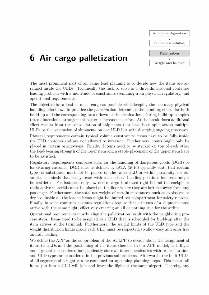
6 Air cargo palletization
Aircraft configuration
Build-up scheduling
Palletization
Weight and balance
The most prominent part of air cargo load planning is to decide how the items are ar-ranged inside the ULDs. Technically the task to solve is a three-dimensional containerloading problem with a multitude of constraints stemming from physical, regulatory, andoperational requirements.The objective is to load as much cargo as possible while keeping the necessary physicalhandling effort low. In practice the palletization determines the handling efforts for bothbuild-up and the corresponding break-down at the destination. During build-up complexthree-dimensional arrangement patterns increase the effort. At the break-down additionaleffort results from the consolidation of shipments that have been split across multipleULDs or the separation of shipments on one ULD but with diverging ongoing processes.Physical requirements contain typical volume constraints: items have to be fully insidethe ULD contours and are not allowed to intersect. Furthermore, items might only beplaced in certain orientations. Finally, if items need to be stacked on top of each otherthe load-bearing strength of the lower item and a stable placement of the upper item haveto be satisfied.Regulatory requirements comprise rules for the handling of dangerous goods (DGR) orfor clearing customs. DGR rules as defined by IATA (2016) typically state that certaintypes of substances must not be placed on the same ULD or within proximity, for ex-ample, chemicals that easily react with each other. Loading positions for items mightbe restricted. For instance, only low dense cargo is allowed right behind the cockpit orradio-active materials must be placed on the floor where they are farthest away from anypassenger. Furthermore, the total net weight of certain substances, such as explosives ordry ice, inside all the loaded items might be limited per compartment for safety reasons.Finally, in some countries customs regulations require that all items of a shipment mustarrive with the same flight, effectively creating an all or nothing rule for the airline.Operational requirements mostly align the palletization result with the neighboring pro-cess steps. Items need to be assigned to a ULD that is scheduled for build-up after theitem arrives at the terminal. Furthermore, the weight limits of the ULD type and theweight distribution limits inside each ULD must be respected, to allow easy and error freeaircraft loading.We define the APP as the subproblem of the ACLPP to decide about the assignment ofitems to ULDs and the positioning of the items therein. In our APP model, each flightand segment is considered independently since all interdependencies with respect to timeand ULD types are considered in the previous subproblems. Afterwards, the built ULDsof all segments of a flight can be combined for upcoming planning steps. This means allitems put into a ULD will join and leave the flight at the same airport. Thereby, any
6 Air cargo palletization
multi-drop restriction is postponed to the weight and balance step, which we present inChapter 7. The input parameters of the APP are the item and ULD attributes as wellas a set of palletization rules. We refrain from modeling logically similar domain specificrules, like net weights or sorting constraints, individually. Instead we present them in anabstract format that can be instantiated as needed.In the next section, we discuss literature related to the APP followed by a mathematicalformulation of the problem in Section 6.2.
6.1 Related literature
There is a vast amount of literature regarding container loading problems. Bortfeldt andWäscher (2013) present a recent review of more than 160 papers. They categorize theworks by their objective, heterogeneity of the considered objects, and constraints. Pollariset al. (2015) update this review and focus on vehicle routing problems. Thereby, theyexplicitly highlight papers with an aircraft loading context.According to these reviews, the typical objectives of container loading problems are eitherto minimize the used number of bins, referred to as input minimization, or maximizingthe utilization of a given set of bins, referred to as output maximization. The problemconsidered in this work combines both objectives. If all items can be loaded, the number ofbins should be small to save handling operations. But, if the aircraft capacity is exceeded,all bins will be used and as many items as possible should be loaded.Furthermore, Bortfeldt and Wäscher (2013) characterize the problems by the level ofheterogeneity of the items and bins. In this respect, the APP falls into the category ofstrongly heterogeneous items with heterogeneous bins, classified as Multiple Bin-Size BinPacking Problem (MBSBPP) and Multiple Heterogeneous Knapsack Problem (MHKP).According to an earlier classification by Hodgson (1982) the APP represents a classicaldistributors packing problem.In Bischoff and Ratcliff (1995) the authors describe a set of twelve practical requirements ofpacking problems: individual allowed item orientations, maximum load-bearing strengthof each item, item positioning inside/outside a certain area, physical stability when stack-ing items, grouping items into the same bin, multi-drop accessibility, item separation,complete shipment, item priorities, complexity of loading arrangements, maximum binweight, and weight distribution inside each bin. Except for multi-drop restrictions all therequirements are present in the APP. A ULD with multiple drops is usually not feasible.In general, ULDs cannot be opened or altered inside the aircraft and the effort of tem-porary unloading a ULD from the aircraft is quite high. Multi-drop constraints betweendifferent ULDs in the aircraft are considered during weight and balance in Chapter 7.There we assign suitable loading positions and hence decide about the loading order.Bortfeldt and Wäscher (2013) pick up the classification presented above and correlate therecent literature to it. They state that there has been only little research that simultane-ously deals with multiple types of practical constraints. However, there are a few paperson general bin packing problems that cover at least some of the constraints present inour problem. Techanitisawad and Tangwiwatwong (2004) and Lin et al. (2006) presenttwo-step solutions: first they distribute items across the bins by solving a MIP model
40
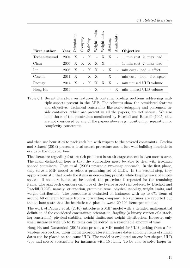
6.1 Related literature
First author Year Orie
ntation
Group
ing
Stab
ility
Weigh
tlim
its
Weigh
tdistr.
Stacking
Availability
ObjectiveTechanitisawad 2004 X - X - X X - 1. min cost, 2. max loadChan 2006 X X X X X - - 1. min cost, 2. max loadLin 2006 X - X X - X - min cost - load + effortCeschia 2011 X - X X - X - min cost - load - free spacePaquay 2014 X - X X X X - min unused ULD volumeHong Ha 2016 - - - X - - X min unused ULD volume
Table 6.1: Recent literature on feature-rich container loading problems addressing mul-tiple aspects present in the APP. The columns show the considered featuresand objective. Technical constraints like non-overlapping and placement in-side container, which are present in all the papers, are not shown. We alsoomit those of the constraints mentioned by Bischoff and Ratcliff (1995) thatare not considered by any of the papers above, e.g., positioning, separation, orcomplexity constraints.
and then use heuristics to pack each bin with respect to the covered constraints. Ceschiaand Schaerf (2013) present a local search procedure and a fast wall-building heuristic toevaluate the updated bins.The literature regarding feature-rich problems in an air cargo context is even more scarce.The main distinction here is that the approaches must be able to deal with irregularshaped containers. Chan et al. (2006) present a two-stage approach. In the first phase,they solve a MIP model to select a promising set of ULDs. In the second step, theyapply a heuristic that loads the items in descending priority while keeping track of emptyspaces. If no more items can be loaded, the procedure is repeated for the remainingitems. The approach considers only five of the twelve aspects introduced by Bischoff andRatcliff (1995), namely: orientation, grouping items, physical stability, weight limits, andweight distribution. The procedure is evaluated on instances with up to 671 items ofaround 50 different formats from a forwarding company. No runtimes are reported butthe authors state that the heuristic can place between 20-100 items per minute.The work of Paquay et al. (2016) introduces a MIP model with a detailed mathematicaldefinition of the considered constraints: orientation, fragility (a binary version of a stack-ing constraint), physical stability, weight limits, and weight distribution. However, onlysmall instances with up to 12 items can be solved in a reasonable amount of time.Hong Ha and Nananukul (2016) also present a MIP model for ULD packing from a for-warders perspective. Their model incorporates item release dates and only items of similardates can be placed on the same ULD. The model is evaluated on one box-shaped ULDtype and solved successfully for instances with 15 items. To be able to solve larger in-
41

6 Air cargo palletization
stances the authors relax the three-dimensional constraints and instead cap the maximumvolume utilization of the ULDs. The three-dimensional packing is then solved for eachULD in a separate postprocessing step. If no feasible solution is found for a ULD, themain MIP model is solved again with a reduced utilization cap.Some more papers deal with palletization problems from a forwarders view: Wu (2008)presents a MIP model and Lau et al. (2009) a genetic algorithm to select ULDs and assignitems to them. However, they do not consider practical constraints. Both papers aim tominimize the rental and transport fees of the built ULDs.Moreover, there exist papers considering packing problems in air cargo in the military do-main like Heidelberg et al. (1998), Guéret et al. (2003), and Nance et al. (2011). However,these problems are fundamentally different because the loaded cargo is homogeneous oris not placed on ULDs such as trucks or large machinery, which are loaded directly.To sum up, there is a large number of publications regarding container loading and themajority of practical constraints is known. But, all the works are missing importantaspects of our problem at hand and only cover parts of the constraints. We give anoverview of the mentioned papers, their covered features and objectives in Table 6.1.
6.2 The Air Cargo Palletization Model
In this section, we define a mathematical model of the APP, which we denote as theAir Cargo Palletization Model (APM) in the following. Its goal is to find an assignmentand arrangement of the items into ULDs, while respecting the physical, regulatory, andoperational constraints. As the majority of items are box-shaped, we only deal withcuboid items here. Accordingly, we model irregular items, cylinders or sacks by theircuboid bounding box with a suitable load-bearing strength.The basis for our model is the one given by Paquay et al. (2016). Our model contains somekey features that have, to the best of our knowledge, not been presented in literature:• We introduce time as a new dimension of packing problems. Each item has an
individual period at which it becomes available for loading. All ULDs have anindividual due date at which they will be built. Consequently, only items that areavailable before the due date of a ULD can be assigned to it.• Next to the item gross weight, we introduce a set of net weights for each item.
These typically represent DGR substances, e.g., dry ice, explosives, or radio-activematerials, whose total weight inside certain ULD subsets must be limited.• We present a formal definition of a load-bearing constraint that allows items to be
stacked with partial support and calculates how the weight is transmitted betweenthe items.• In practice, stacked items do not need a perfectly even surface. It is also acceptable if
the items below vary slightly in their height. Therefore we add a tolerance parameterε and allow stacked items to float "in the air" within the tolerance.• We use a single coordinate system for all ULDs, which allows for an easy integration
of item separation and positioning constraints.
42

6.2 The Air Cargo Palletization Model
• To facilitate fine-grained item sorting, we add soft allocation constraints that canbe seen from two perspectives. On the one hand, we want to split a group of itemsacross as few ULDs as possible. On the other hand, we want to load only fewdifferent groups of items into a ULD.
We start by defining the input parameters and decision variables followed by the problem’sconstraints and objective. At last, we present a short overview of the model.
6.2.1 Parameters
The APM primarily contains two sets of entities, items I and ULDs U , and considers atime horizon t. To describe the constraints we introduce another three sets of entities:• Rotations R: We consider only orthogonal item rotations. Each rotation is de-
scribed by its permutation of item dimensions. Accordingly, there are six possiblerotations: R = {XYZ,XZY,YXZ,YZX,ZXY,ZYX}. XYZ is the original item rota-tion. For example, rotation ZYX represents a turn by 90 degrees around the y-axis.In this case the item’s z-axis corresponds to the bin’s x-axis and vice versa.• Sorting criteria Q: During palletization we want to group or separate certain
items. For example items of the same shipment should be grouped together, whileexpress items should be kept separate from standard items. Each sorting criteriondescribes such a constraint to group or separate by. For each criterion q ∈ Q let Qq
denote the union of groups all the considered items belong to.• Weight categories G: Besides the gross weight of each item we need to consider
the net weight of certain substances inside the items. Each considered substancelike dry ice or explosives represents a weight category.
In the following we use the respective lower case indices to represent single entities: g ∈ G,i, j ∈ I, u ∈ U , q ∈ Q, r ∈ R, t ∈ T .
Item parameters• A ⊆ I × I: pairs of items that are not allowed within one ULD (〈i, j〉 ∈ A)• availi ∈ T : first period that item i is physically available for build-up• cliquei ∈ I: item that must be loaded iff item i is loaded• dimx
i , dimyi , dimz
i ∈ R≥0: dimensions of item i
• disti,j ∈ R≥0: minimum required distance between items i and j• offloadi ∈ R≥0: penalty when item i is offloaded• roti ⊆ R: allowed rotations of item i
• sortq,i ∈ Qq: group of item i for sorting criterion q• suppi ∈ [0, 1]: minimum required supported floor area of item i (ratio)• stackxi , stack
yi , stackzi ∈ R≥0: maximum load-bearing strength of item i
• Ui ⊆ U : ULDs that item i can be loaded into• weightgrsi ∈ R≥0: gross weight of item i
• weightnetg,i ∈ R≥0: net weight of item i for weight category g
43
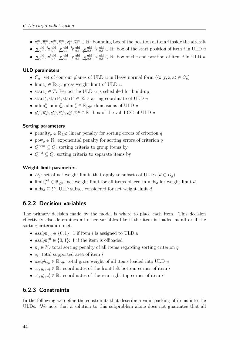
6 Air cargo palletization
• xaci , xaci , yaci , yaci , zaci , zaci ∈ R: bounding box of the position of item i inside the aircraft• x←−
uldu,i ,←−x uld
u,i , y←−uldu,i ,←−y uld
u,i , z←−uldu,i ,←−z uld
u,i ∈ R: box of the start position of item i in ULD u
• x−→uldu,i ,−→x uld
u,i , y−→uldu,i ,−→y uld
u,i , z−→uldu,i ,−→z uld
u,i ∈ R: box of the end position of item i in ULD u
ULD parameters• Cu: set of contour planes of ULD u in Hesse normal form (〈x, y, z, a〉 ∈ Cu)• limitu ∈ R≥0: gross weight limit of ULD u
• startu ∈ T : Period the ULD u is scheduled for build-up• startxu, startyu, startzu ∈ R: starting coordinate of ULD u
• udimzu, udimy
u, udimxu ∈ R≥0: dimensions of ULD u
• xcgu , xcgu , ycgu , ycgu , zcgu , zcgu ∈ R: box of the valid CG of ULD u
Sorting parameters• penaltyq ∈ R≥0: linear penalty for sorting errors of criterion q• powq ∈ N: exponential penalty for sorting errors of criterion q• Qitem ⊆ Q: sorting criteria to group items by• Quld ⊆ Q: sorting criteria to separate items by
Weight limit parameters• Dg: set of net weight limits that apply to subsets of ULDs (d ∈ Dg)• limitnetd ∈ R≥0: net weight limit for all items placed in uldsd for weight limit d• uldsd ⊆ U : ULD subset considered for net weight limit d
6.2.2 Decision variables
The primary decision made by the model is where to place each item. This decisioneffectively also determines all other variables like if the item is loaded at all or if thesorting criteria are met.• assignu,i ∈ {0, 1}: 1 if item i is assigned to ULD u
• assignoffi ∈ {0, 1}: 1 if the item is offloaded
• nq ∈ N: total sorting penalty of all items regarding sorting criterion q• oi: total supported area of item i
• weightu ∈ R≥0: total gross weight of all items loaded into ULD u
• xi, yi, zi ∈ R: coordinates of the front left bottom corner of item i
• x′i, y′i, z′i ∈ R: coordinates of the rear right top corner of item i
6.2.3 Constraints
In the following we define the constraints that describe a valid packing of items into theULDs. We note that a solution to this subproblem alone does not guarantee that all
44

6.2 The Air Cargo Palletization Model
planned ULDs can be loaded into the aircraft. Further constraints regarding the aircraftloading are presented in Chapter 7. Along the upcoming constraints further auxiliaryvariables are defined that are only relevant inside the defining constraint.
ULD assignment Each item i needs either be assigned to a compatible ULD from theset Ui or marked as offloaded:
assignoffi +
∑u∈Ui
assignu,i = 1 i ∈ I (6.1)
Item orientation and size The rotation of each item determines the effective size ofthe item in each dimension. Therefore, we combine the calculation of the start and endcoordinates of each item with the determination of its rotation. To describe the rotationof item i, we use a 3 × 3 rotation matrix ri of auxiliary binary decision variables. Thefollowing examples show such a matrix representing the original item orientation XYZand a horizontal rotation around the y-axis ZYX:
XYZ =
1 0 00 1 00 0 1
ZYX =
0 0 10 1 01 0 0
(6.2)
By using the coordinates of the front left bottom corner (xi, yi, zi) of item i, its dimensions(dimx
i , dimyi , dimz
i ) and the rotation matrix of the item, we calculate the coordinates ofthe rear right top corner (x′i, y′i, z′i) of item i as follows:xiyi
zi
+
r11i r12
i r13i
r21i r22
i r23i
r31i r32
i r33i
dim
xi
dimyi
dimzi
=
x′i
y′iz′i
i ∈ I (6.3)
To give a complete example, let us assume item i has orientation ZYX. Then, the itemdimensions along the x- and z-axis are flipped and the rear right top corner is calculatedas follows:xiyi
zi
+ ZY X
dimxi
dimyi
dimzi
=
xiyizi
+
0 0 10 1 01 0 0
dim
xi
dimyi
dimzi
=
xi + dimzi
yi + dimyi
zi + dimxi
=
x′i
y′iz′i
(6.4)
The matrix only contains a valid orthogonal rotation if each row and column of the matrixcontains exactly one 1. Accordingly, we add the following constraints for each row andcolumn:
3∑b=1
rabi = 1 i ∈ I; a ∈ {1, 2, 3} (6.5)
3∑a=1
rabi = 1 i ∈ I; b ∈ {1, 2, 3} (6.6)
Finally, we restrict the rotation matrix to rotations that are explicitly allowed for item i:
XYZ /∈ roti ⇒ r11i + r22
i + r33i ≤ 1 i ∈ I (6.7)
45
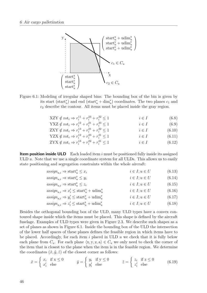
6 Air cargo palletization
startxustartyustartzu
startxu + udimxu
startyu + udimyu
startzu + udimzu
x
y
c1 ∈ Cu
c2 ∈ Cu
Figure 6.1: Modeling of irregular shaped bins: The bounding box of the bin is given byits start (start∗u) and end (start∗u + dim∗u) coordinates. The two planes c1 andc2 describe the contour. All items must be placed inside the gray region.
XZY /∈ roti ⇒ r11i + r23
i + r32i ≤ 1 i ∈ I (6.8)
YXZ /∈ roti ⇒ r12i + r21
i + r33i ≤ 1 i ∈ I (6.9)
ZXY /∈ roti ⇒ r13i + r21
i + r32i ≤ 1 i ∈ I (6.10)
YZX /∈ roti ⇒ r12i + r23
i + r31i ≤ 1 i ∈ I (6.11)
ZYX /∈ roti ⇒ r13i + r22
i + r31i ≤ 1 i ∈ I (6.12)
Item position inside ULD Each loaded item imust be positioned fully inside its assignedULD u. Note that we use a single coordinate system for all ULDs. This allows us to easilystate positioning and segregation constraints within the whole aircraft:
assignu,i ⇒ startxu ≤ xi i ∈ I;u ∈ U (6.13)assignu,i ⇒ startyu ≤ yi i ∈ I;u ∈ U (6.14)assignu,i ⇒ startzu ≤ zi i ∈ I;u ∈ U (6.15)assignu,i ⇒ x′i ≤ startxu + udimx
u i ∈ I;u ∈ U (6.16)assignu,i ⇒ y′i ≤ startyu + udimy
u i ∈ I;u ∈ U (6.17)assignu,i ⇒ z′i ≤ startzu + udimz
u i ∈ I;u ∈ U (6.18)
Besides the orthogonal bounding box of the ULD, many ULD types have a convex con-toured shape inside which the items must be placed. This shape is defined by the aircraftfuselage. Examples of ULD types were given in Figure 2.3. We describe such shapes as aset of planes as shown in Figure 6.1. Inside the bounding box of the ULD the intersectionof the lower half spaces of these planes defines the feasible region in which items have tobe placed. Accordingly, for each item i placed in ULD u we check that it is fully beloweach plane from Cu. For each plane 〈x, y, z, a〉 ∈ Cu we only need to check the corner ofthe item that is closest to the plane when the item is in the feasible region. We determinethe coordinates (x, y, z) of the closest corner as follows:
x ={xi if x ≤ 0x′i else y =
{yi if y ≤ 0y′i else z =
{zi if z ≤ 0z′i else (6.19)
46
6.2 The Air Cargo Palletization Model
The following constraint ensures that the item is placed in the feasible region:
xx+ yy + zz ≤ a (6.20)
Item non-overlapping If two items i, j are loaded, then their positions must not overlap.Note that this constraint is independent of the assigned ULD because all ULDs share thesame coordinate system in our model. We describe the position of item i by its front leftbottom corner (xi, yi, zi) and its rear right top corner (x′i, y′i, z′i). The two items i, j donot overlap with respect to a certain dimension if i is either in front of j (x′i ≤ xj) fordimension x or behind j (x′j ≤ xi). In three-dimensional space items do not overlap ifthey do not overlap in any dimension. Accordingly, we formulate the following constraint:
¬(assignoffi ∨ assignoff
j )⇒
x′i ≤ xj ∨ x′j ≤ xi∨y′i ≤ yj ∨ y′j ≤ yi∨z′i ≤ zj ∨ z′j ≤ zi
i, j ∈ I (6.21)
Item availability Each item i can only be assigned to a ULD u whose build-up periodstartu is not before the item arrival time availi. For transferred items, availi can bedetermined by the inbound connection plus a suitable transfer time. For items deliveredto the terminal by the customer the parameter can be derived from the agreed hand-overtime.
availiassignu,i ≤ startu u ∈ U ; i ∈ I (6.22)
ULD weight limit For each ULD u the sum of the item gross weights weightgrsi of allitems placed on the ULD is limited. We expect that the weight limit limitu is alreadyadjusted to allow for the weight of the ULD itself, the weight of the covering net andstraps, the weight of possibly necessary additional loading devices like wooden boards, aswell as a suitable tolerance. We calculate the total weight of the ULD as weightu and willreuse it in the upcoming weight distribution constraint.
∑i∈I
weightgrsi assignu,i = weightu u ∈ U (6.23)
weightu ≤ limitu u ∈ U (6.24)
Net weight limits Besides the gross weight of each item, some items may contain sub-stances (dry ice, radiation, chemicals, explosives) whose total sum needs to be limitedwithin a subset of ULDs, typically all ULDs that will be put into the same compartmentof the aircraft, for safety reasons.We denote the set of restricted substances as G and the constraints related to substanceg ∈ G as Dg. For each constraint d ∈ Dg the subset of ULDs in which the substance mustbe limited is given as uldsd. The weight limit itself is given as limitnetd . We denote thenet weight of substance g inside item i as weightnetg,i . The loaded net weights can now berestricted as follows:∑
u∈uldsd
∑i∈I
weightnetg,i assignu,i ≤ limitnetd g ∈ G; d ∈ Dg (6.25)
47
6 Air cargo palletization
ULD weight distribution For safety reasons, the items must be packed in a way suchthat the center of gravity (CG) of each ULD u is within a defined bounding box. Wedenote the coordinates of the front left bottom corner of this bounding box as (xcgu , ycgu , zcgu )and the rear right top corner as (xcgu , ycgu , zcgu ). As a simplification, we assume that the CGof each item is at its geometric center. In dimension x, for example, this geometric centercan be calculated as (xi + x′i)/2. To determine the CG of a set of items for a dimensionwe calculate the weighted sum of their geometric centers. Accordingly, for dimension xthe CG can be calculated as:
∑i
(weightgrsi
total weight
)(xi + x′i
2
)(6.26)
To limit the weight distribution inside the ULD u, we restrict the CG for each dimensionto stay within the defined bounding box (xcgu , ycgu , zcgu )− (xcgu , ycgu , zcgu ). Only items loadedinto the ULD u need to be considered which is indicated by variable assignu,i. From theULD weight limit constraint we know the total weight of the loaded items weightu. TheCG can now be restricted for each dimension as follows:
xcgu ≤1
2weightu
∑i∈I
weightgrsi (xi + x′i) assignu,i ≤ xcgu u ∈ U (6.27)
ycgu ≤1
2weightu
∑i∈I
weightgrsi (yi + y′i) assignu,i ≤ ycgu u ∈ U (6.28)
zcgu ≤1
2weightu
∑i∈I
weightgrsi (zi + z′i) assignu,i ≤ zcgu u ∈ U (6.29)
Stacking When loading multiple items into the same ULD, some items might have tobe stacked on top of others. As most items carry significant weight and the load-bearingstrength of each item is limited, we need to properly restrict the stacking in our model.Modeling exact stacking constraints is hard for two reasons. First, modeling the dynamicsbetween stacked items is usually done via finite element simulations. Integrating such asimulation into any optimization model would most probably render it impossible to solve.Second, the real load-bearing strength of each item is seldom known, it depends on wherethe forces act, at the center or along the edges, and it cannot easily be determined withoutbreaking the item.Therefore, we model a simplified stacking constraint that considers only vertical forcesand no torque. We assume that an item’s weight is equally distributed across its volumeand that the load-bearing strength is the same all across the top surface. Each item passesits weight onto the items below proportional to their overlapping area. The item belowadds the received weight to its own weight and again passes the sum to the items below.This way, we can calculate the stress, i.e., the weight per area unit, transferred betweentwo items and limit it to an acceptable level.Figure 6.2 gives an example how the stacking restriction works. There are four items withdifferent weights (A: 100 kg, B: 500 kg, C: 600 kg, D: 1,000 kg). Item A has no items ontop, so its total weight is 100 kg. It passes its weight to item B resulting in a pressure of50 kg ·m−1 at the contact area. The total weight of item B is 600 kg, the weight received
48
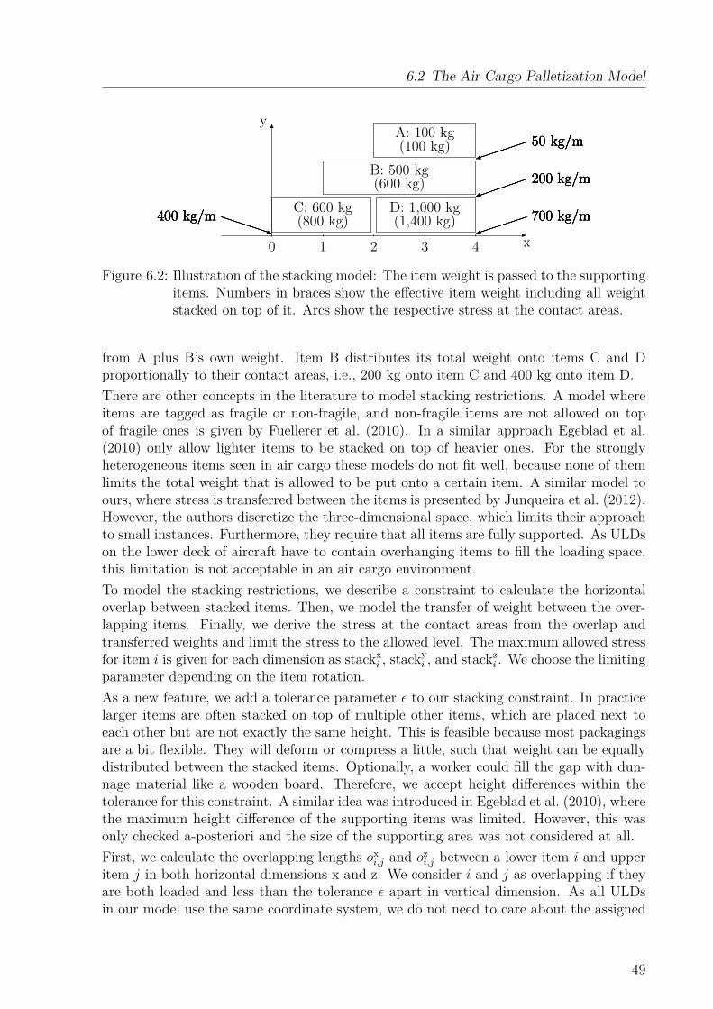
6.2 The Air Cargo Palletization Model
C: 600 kg(800 kg)
D: 1,000 kg(1,400 kg)
B: 500 kg(600 kg)
A: 100 kg(100 kg)
y
x0
50 kg/m
200 kg/m
700 kg/m400 kg/m
1
50 kg/m
200 kg/m
700 kg/m400 kg/m
2
50 kg/m
200 kg/m
700 kg/m400 kg/m
3
50 kg/m
200 kg/m
700 kg/m400 kg/m
4
50 kg/m
200 kg/m
700 kg/m400 kg/m
Figure 6.2: Illustration of the stacking model: The item weight is passed to the supportingitems. Numbers in braces show the effective item weight including all weightstacked on top of it. Arcs show the respective stress at the contact areas.
from A plus B’s own weight. Item B distributes its total weight onto items C and Dproportionally to their contact areas, i.e., 200 kg onto item C and 400 kg onto item D.There are other concepts in the literature to model stacking restrictions. A model whereitems are tagged as fragile or non-fragile, and non-fragile items are not allowed on topof fragile ones is given by Fuellerer et al. (2010). In a similar approach Egeblad et al.(2010) only allow lighter items to be stacked on top of heavier ones. For the stronglyheterogeneous items seen in air cargo these models do not fit well, because none of themlimits the total weight that is allowed to be put onto a certain item. A similar model toours, where stress is transferred between the items is presented by Junqueira et al. (2012).However, the authors discretize the three-dimensional space, which limits their approachto small instances. Furthermore, they require that all items are fully supported. As ULDson the lower deck of aircraft have to contain overhanging items to fill the loading space,this limitation is not acceptable in an air cargo environment.To model the stacking restrictions, we describe a constraint to calculate the horizontaloverlap between stacked items. Then, we model the transfer of weight between the over-lapping items. Finally, we derive the stress at the contact areas from the overlap andtransferred weights and limit the stress to the allowed level. The maximum allowed stressfor item i is given for each dimension as stackxi , stack
yi , and stackzi . We choose the limiting
parameter depending on the item rotation.As a new feature, we add a tolerance parameter ε to our stacking constraint. In practicelarger items are often stacked on top of multiple other items, which are placed next toeach other but are not exactly the same height. This is feasible because most packagingsare a bit flexible. They will deform or compress a little, such that weight can be equallydistributed between the stacked items. Optionally, a worker could fill the gap with dun-nage material like a wooden board. Therefore, we accept height differences within thetolerance for this constraint. A similar idea was introduced in Egeblad et al. (2010), wherethe maximum height difference of the supporting items was limited. However, this wasonly checked a-posteriori and the size of the supporting area was not considered at all.First, we calculate the overlapping lengths oxi,j and ozi,j between a lower item i and upperitem j in both horizontal dimensions x and z. We consider i and j as overlapping if theyare both loaded and less than the tolerance ε apart in vertical dimension. As all ULDsin our model use the same coordinate system, we do not need to care about the assigned
49

6 Air cargo palletization
ULD of each item.
¬(assignoff
i ∨ assignoffj
)∧ (0 ≤ yj − y′i ≤ ε)⇒
oxi,j = max(0,min(x′i, x′j)−max(xi, xj))i, j ∈ I (6.30)
¬(assignoff
i ∨ assignoffj
)∧ (0 ≤ yj − y′i ≤ ε)⇒
ozi,j = max(0,min(z′i, z′j)−max(zi, zj))i, j ∈ I (6.31)
From the overlaps we calculate the total supported area oj of each item j as follows. Wenote that this formulation is non-linear, making this part of the problem intractable forplain LP solving.
oj =∑i∈I
oxi,jozi,j j ∈ I (6.32)
We now model the transfer of weight from upper items j to lower item i. Even if the upperitem is not fully supported, our formulation ensures that all the weight of an upper itemis transferred to the items below it. We introduce an auxiliary variable wi representingthe total weight of item i, which is the sum of the weight of the lower item i plus theweight transferred to it by items above.
wi = weightgrsi +∑j∈I
oxi,jozi,j
ojwj i ∈ I (6.33)
Finally, we restrict the stress of an upper item j onto lower item i by the load-bearingstrength of the vertical orientation of item i. To detect the vertical orientation we reuseauxiliary variables r2∗
i from the rotation matrix of the item orientation constraint. Wedetermine the stress at the contact area by the total weight and the total supported areaof the item above.
oxi,jozi,j > 0⇒ r21
i stackxi + r22i stackyi + r23
i stackzi ≥wjoj
i, j ∈ I (6.34)
Complete shipment There are different variations of complete shipment constraints.According to the classification given by Eley (2003), the problem at hand is of the typewhere subsets of boxes have to be either all loaded or left out completely.Shipments may consist of multiple items that can in theory be shipped individually. But,in some countries customs regulations do not permit the arrival of partial shipments. Insuch countries the airline has to pay a considerable fine if not all items of a shipmentarrive with the same flight. Accordingly, we introduce a constraint that either all or noitems of a certain group are loaded.Therefore, we select one item of each shipment to represent the group that belongs to-gether. Each item i has a parameter cliquei pointing to the master item of its group.For each item we force the offload variable assignoff
i to be equal to the same variable ofthe group’s master item. This effectively creates a clique where either all or no items areloaded.
assignoffi = assignoff
cliqueii ∈ I (6.35)
50

6.2 The Air Cargo Palletization Model
Item sorting Besides the requirement to load only complete shipments, airlines alsowant to spread a shipment with multiple items across as few ULDs as possible. Thisdecreases the risk of disruptions, e.g., if a ULD does not catch its flight, and reduces thehandling effort to consolidate the shipment again at the destination. In practice thereare even more reasons to reduce the spread of a set of items across ULDs. For exampleitems that arrive with the same inbound flight at the terminal, that have the same finaldestination, or items that need special care during flight, like animals. Placing these itemson only a few ULDs saves a lot of handling effort.Item sorting can also be seen from a ULD perspective. Air cargo is often offered withdifferent service levels, say standard and premium. As the premium shipments are soldwith the promise to be processed faster at the destination airport, they should not bemixed with standard cargo. Another good reason for item sorting is to fill a ULD onlywith items that have the same connecting flight after the current one. In this case, aso called thru-unit can be built that can transit the next station without requiring anyhandling effort.While these are different requirements from a business view, they are technically equiv-alent. Therefore, we formulate them all in the same way in our model. We identify twovantage points on the sorting criteria. The first is item-bound: a group of items shouldbe split across as few ULDs as possible. The other is ULD-bound: inside one ULD thereshould be as few different item groups as possible. We denote the corresponding criteriasets as Quld and Qitem (Q = Quld ∪ Qitem). For each sorting criterion q ∈ Q each item ihas a parameter sortq,i ∈ Qq indicating the group it belongs to with respect to criterionq. We add auxiliary variables sortq,u,e for each constraint q indicating if the item groupe ∈ Qq is present in ULD u. This is the case if any item of this group is assigned to u:
assignu,i ≤ sortq,u,e q ∈ Q;u ∈ U ; e ∈ Qq; i ∈ I : sortq,i = e (6.36)
To calculate the degree of sorting nq for each item-bound constraint q we count the numberof ULDs each group is present in. To better express the impact of bad sorting for eachconstraint we add an exponential penalty parameter powq. We note that this non-linearrestriction can be reformulated into piecewise linear restrictions because the number ofULDs a group is spread across will usually be small. We calculate the degree of sortingas:
nq =∑e∈Qq
(∑u∈U
sortq,u,e)powq
q ∈ Qitem (6.37)
To calculate the degree of sorting for ULD-bound constraints, we sum up the same inci-dence matrix as above just in the opposite order of dimensions:
nq =∑u∈U
∑e∈Qq
sortq,u,e
powq
q ∈ Quld (6.38)
Item compatibility Besides the soft item grouping constraints, there are also hard con-straints on items, which must not be placed on the same ULD or in close proximity. Theseconstraints mostly stem from official dangerous goods regulations (DGR). These define
51

6 Air cargo palletization
a long list of items that have to be separated by a minimum distance. Examples arefood and perfumery items, animals and items containing sources of radiation, or itemswith chemicals that could react with each other. There is only one paper by Eley (2003)dealing with this kind of item separation constraint.To split incompatible items onto different ULDs we introduce a constraint for all pairs〈i, j〉 of incompatible items A:
assignu,i + assignu,j ≤ 1 u ∈ U ; 〈i, j〉 ∈ A (6.39)
Item spacing For pairs of items that require a certain minimum distance we introducea parameter disti,j. Remember the coordinates of item i: the front bottom left corner(xi, yi, zi) end the rear top right corner (x′i, y′i, z′i). For this constraint we consider hor-izontal distance only, because vertical distance might not be sufficient for leakages. Tosimplify the model we calculate the Manhattan distance instead of Euclidean distance be-tween the items. Furthermore, multiplying a Euclidean distance by a factor of
√2 yields
a valid upper bound for the distance in Manhattan distance. We define the minimumdistance constraint between two items i and j as:
max(0, xi − x′j, xj − x′i) + max(0, zi − z′j, zj − z′i) ≥√
2disti,j i, j ∈ I (6.40)
Item positioning For some items the allowed position inside the aircraft or inside theassigned ULD needs to be restricted.For example, if radioactive materials are loaded into a passenger aircraft they must havea minimum distance to the passengers’ cabin, i.e., be loaded not above a certain absoluteheight. To model a global positioning constraint of item i we introduce a bounding box(xaci , yaci , zaci ) to (xaci , yaci , zaci ). The item’s position has to stay within this box:
xaci ≤ xi i ∈ I (6.41)x′i ≤ xaci i ∈ I (6.42)yaci ≤ yi i ∈ I (6.43)y′i ≤ yaci i ∈ I (6.44)zaci ≤ zi i ∈ I (6.45)z′i ≤ zaci i ∈ I (6.46)
Similarly, the relative position of an item inside the ULD might need to be constrained.This is usually the case for dangerous goods that need to be placed on the periphery ofthe ULD to be inspected or accessed if necessary. The same applies to living animals thatneed ventilation. On the other hand, items of high value should not be placed on theperiphery to prevent theft. To model this constraint of item i when assigned to ULD u weintroduce two more bounding boxes, one for the item start coordinates ( x←−
uldu,i , y←−
uldu,i , z←−
uldu,i )
to (←−x uldu,i ,←−y uld
u,i ,←−z uld
u,i ) and another for the item end coordinates ( x−→uldu,i , y−→
uldu,i , z−→
uldu,i ) to
(−→x uldu,i ,−→y uld
u,i ,−→z uld
u,i ). We apply the Big M method to relax this constraint if the itemis offloaded at all. The relative position is then limited as:
xi ≥ x←−uldu,i + (assignu,i − 1)M u ∈ U ; i ∈ I (6.47)
52

6.2 The Air Cargo Palletization Model
xi ≤ ←−x uldu,i + (1− assignu,i)M u ∈ U ; i ∈ I (6.48)
yi ≥ y←−uldu,i + (assignu,i − 1)M u ∈ U ; i ∈ I (6.49)
yi ≤ ←−y uldu,i + (1− assignu,i)M u ∈ U ; i ∈ I (6.50)
zi ≥ z←−uldu,i + (assignu,i − 1)M u ∈ U ; i ∈ I (6.51)
zi ≤ ←−z uldu,i + (1− assignu,i)M u ∈ U ; i ∈ I (6.52)
x′i ≥ x−→uldu,i + (assignu,i − 1)M u ∈ U ; i ∈ I (6.53)
x′i ≤ −→x uldu,i + (1− assignu,i)M u ∈ U ; i ∈ I (6.54)
y′i ≥ y−→uldu,i + (assignu,i − 1)M u ∈ U ; i ∈ I (6.55)
y′i ≤ −→y uldu,i + (1− assignu,i)M u ∈ U ; i ∈ I (6.56)
z′i ≥ z−→uldu,i + (assignu,i − 1)M u ∈ U ; i ∈ I (6.57)
z′i ≤ −→z uldu,i + (1− assignu,i)M u ∈ U ; i ∈ I (6.58)
Stability Load stability is required for all ULDs to prevent damage of the cargo andmovements inside the aircraft, which would endanger flight safety. We distinguish betweenvertical and horizontal stability. Vertical stability prevents the items from falling downor tipping. To enforce vertical stability we require that a minimum ratio suppi of itemi’s floor area is supported by other items or the item is placed directly on the ULD floor.In many papers load stability is assured by requiring full support of all items. In an aircargo setup this often not necessary and sometimes even not possible. For example, ULDson the lower deck only have a small floor area and reach their full width only at around50 cm height. Accordingly, there must be overhanging items to fully utilize the loadingspace.In our formulation the minimum support ratio suppi is item dependent, because differentitem geometries might require different supported areas. For a cardboard box with a flatbottom a support of suppi = 0.75 might be sufficient. But, a pallet standing on four feet atits corners only might require full support of suppi = 1.0. For items standing on the ULDfloor we assume full support. Therefore, we assume that items are placed directly on theULD floor if their vertical starting position yi is larger the vertical ULD starting positionstartyu plus the stacking tolerance ε. Accordingly, we restrict the minimum supported areaby the following non-linear constraint:(
yi > assignu,istartyu + ε)⇒ (oi ≥ suppi(x′i − xi)(z′i − zi)) u ∈ U ; i ∈ I (6.59)
Horizontal stability prevents the shifting of items when the ULD is moved or tilted. In aircargo this is usually ensured by the usage of nets and straps after the ULD is build-up.Therefore, we do not model horizontal stability explicitly.
6.2.4 Objective
The objective of the palletization is to load as much as possible while keeping the necessaryphysical handling effort low. Therefore, we penalize all offloaded items, where assignoff
i =1, with their individual penalty offloadi.
53

6 Air cargo palletization
To simplify all handling operations we would also like the load plan to be as sorted aspossible. For each sorting criterion q ∈ Q the variable nq contains a measure how well theitems are sorted. We weight all measures by their individual penalty factors penaltyq.Our objective minimizes the sum of penalties of the offloaded items and violated sortingcriteria:
minimize∑i∈I
offloadiassignoffi +
∑q∈Q
penaltyqnq (6.60)
6.2.5 Model overview
After introducing all components of the APM in the last sections, we now give a consoli-dated view of the full model:
minimize∑i∈I
offloadiassignoffi +
∑q∈Q
penaltyqnq (6.61)
subject to
1 = assignoffi +
∑u∈Ui
assignu,i i ∈ I (6.62)
x′i = xi + r11i dimx
i + r12i dimy
i + r13i dimz
i i ∈ I (6.63)y′i = yi + r21
i dimxi + r22
i dimyi + r23
i dimzi i ∈ I (6.64)
z′i = zi + r31i dimx
i + r32i dimy
i + r33i dimz
i i ∈ I (6.65)
1 =3∑b=1
rabi i ∈ I; a ∈ {1, 2, 3} (6.66)
1 =3∑
a=1rabi i ∈ I; b ∈ {1, 2, 3} (6.67)
XYZ /∈ roti ⇒ r11i + r22
i + r33i ≤ 1 i ∈ I (6.68)
XZY /∈ roti ⇒ r11i + r23
i + r32i ≤ 1 i ∈ I (6.69)
YXZ /∈ roti ⇒ r12i + r21
i + r33i ≤ 1 i ∈ I (6.70)
ZXY /∈ roti ⇒ r13i + r21
i + r32i ≤ 1 i ∈ I (6.71)
YZX /∈ roti ⇒ r12i + r23
i + r31i ≤ 1 i ∈ I (6.72)
ZYX /∈ roti ⇒ r13i + r22
i + r31i ≤ 1 i ∈ I (6.73)
assignu,i ⇒ startxu ≤ xi i ∈ I;u ∈ U (6.74)assignu,i ⇒ startyu ≤ yi i ∈ I;u ∈ U (6.75)assignu,i ⇒ startzu ≤ zi i ∈ I;u ∈ U (6.76)assignu,i ⇒ x′i ≤ startxu + udimx
u i ∈ I;u ∈ U (6.77)assignu,i ⇒ y′i ≤ startyu + udimy
u i ∈ I;u ∈ U (6.78)assignu,i ⇒ z′i ≤ startzu + udimz
u i ∈ I;u ∈ U (6.79)a ≥ xxi + yyi + zzi i ∈ I; 〈x, y, z, a〉 ∈ Cu (6.80)a ≥ xxi + yyi + zz′i i ∈ I; 〈x, y, z, a〉 ∈ Cu (6.81)
54

6.2 The Air Cargo Palletization Model
a ≥ xxi + yy′i + zzi i ∈ I; 〈x, y, z, a〉 ∈ Cu (6.82)a ≥ xxi + yy′i + zz′i i ∈ I; 〈x, y, z, a〉 ∈ Cu (6.83)a ≥ xx′i + yyi + zzi i ∈ I; 〈x, y, z, a〉 ∈ Cu (6.84)a ≥ xx′i + yyi + zz′i i ∈ I; 〈x, y, z, a〉 ∈ Cu (6.85)a ≥ xx′i + yy′i + zzi i ∈ I; 〈x, y, z, a〉 ∈ Cu (6.86)a ≥ xx′i + yy′i + zz′i i ∈ I; 〈x, y, z, a〉 ∈ Cu (6.87)
¬(
assignoffi ∨
assignoffj
)⇒
x′i ≤ xj ∨ x′j ≤ xi∨y′i ≤ yj ∨ y′j ≤ yi∨z′i ≤ zj ∨ z′j ≤ zi
i, j ∈ I (6.88)
startu ≥ availiassignu,i u ∈ U ; i ∈ I (6.89)weightu =
∑i∈I
weightgrsi assignu,i u ∈ U (6.90)
weightu ≤ limitu u ∈ U (6.91)limitnetd ≥
∑u∈uldsd
∑i∈I
weightnetg,i assignu,i g ∈ G; d ∈ Dg (6.92)
2weightuxcgu ≤∑i∈I
weightgrsi (xi + x′i) assignu,i u ∈ U (6.93)
2weightuxcgu ≥∑i∈I
weightgrsi (xi + x′i) assignu,i u ∈ U (6.94)
2weightuycgu ≤∑i∈I
weightgrsi (yi + y′i) assignu,i u ∈ U (6.95)
2weightuycgu ≥∑i∈I
weightgrsi (yi + y′i) assignu,i u ∈ U (6.96)
2weightuzcgu ≤∑i∈I
weightgrsi (zi + z′i) assignu,i u ∈ U (6.97)
2weightuzcgu ≥∑i∈I
weightgrsi (zi + z′i) assignu,i u ∈ U (6.98)
¬(assignoff
i ∨ assignoffj
)∧ (0 ≤ yj − y′i ≤ ε)⇒
oxi,j = max(0,min(x′i, x′j)−max(xi, xj))i, j ∈ I (6.99)
¬(assignoff
i ∨ assignoffj
)∧ (0 ≤ yj − y′i ≤ ε)⇒
ozi,j = max(0,min(z′i, z′j)−max(zi, zj))i, j ∈ I (6.100)
oj =∑i∈I
oxi,jozi,j j ∈ I (6.101)
wi = weightgrsi +∑j∈I
oxi,jozi,j
ojwj i ∈ I (6.102)
oxi,jozi,j > 0⇒ r21
i stackxi + r22i stackyi + r23
i stackzi ≥wjoj
i, j ∈ I (6.103)
assignoffi = assignoff
cliqueii ∈ I (6.104)
assignu,i ≤ sortq,u,sortq,iq ∈ Q;u ∈ U ; i ∈ I (6.105)
55
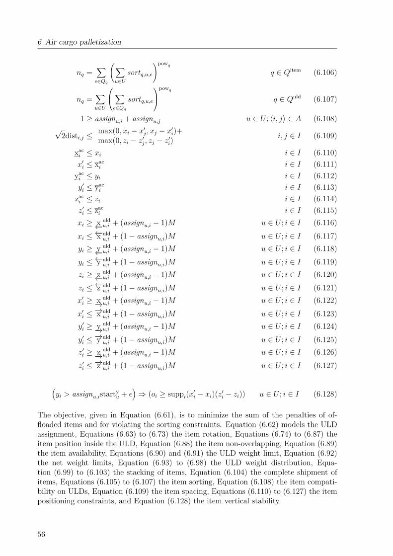
6 Air cargo palletization
nq =∑e∈Qq
(∑u∈U
sortq,u,e)powq
q ∈ Qitem (6.106)
nq =∑u∈U
∑e∈Qq
sortq,u,e
powq
q ∈ Quld (6.107)
1 ≥ assignu,i + assignu,j u ∈ U ; 〈i, j〉 ∈ A (6.108)√
2disti,j ≤max(0, xi − x′j, xj − x′i)+max(0, zi − z′j, zj − z′i)
i, j ∈ I (6.109)
xaci ≤ xi i ∈ I (6.110)x′i ≤ xaci i ∈ I (6.111)yaci ≤ yi i ∈ I (6.112)y′i ≤ yaci i ∈ I (6.113)zaci ≤ zi i ∈ I (6.114)z′i ≤ zaci i ∈ I (6.115)xi ≥ x←−
uldu,i + (assignu,i − 1)M u ∈ U ; i ∈ I (6.116)
xi ≤ ←−x uldu,i + (1− assignu,i)M u ∈ U ; i ∈ I (6.117)
yi ≥ y←−uldu,i + (assignu,i − 1)M u ∈ U ; i ∈ I (6.118)
yi ≤ ←−y uldu,i + (1− assignu,i)M u ∈ U ; i ∈ I (6.119)
zi ≥ z←−uldu,i + (assignu,i − 1)M u ∈ U ; i ∈ I (6.120)
zi ≤ ←−z uldu,i + (1− assignu,i)M u ∈ U ; i ∈ I (6.121)
x′i ≥ x−→uldu,i + (assignu,i − 1)M u ∈ U ; i ∈ I (6.122)
x′i ≤ −→x uldu,i + (1− assignu,i)M u ∈ U ; i ∈ I (6.123)
y′i ≥ y−→uldu,i + (assignu,i − 1)M u ∈ U ; i ∈ I (6.124)
y′i ≤ −→y uldu,i + (1− assignu,i)M u ∈ U ; i ∈ I (6.125)
z′i ≥ z−→uldu,i + (assignu,i − 1)M u ∈ U ; i ∈ I (6.126)
z′i ≤ −→z uldu,i + (1− assignu,i)M u ∈ U ; i ∈ I (6.127)
(yi > assignu,istartyu + ε
)⇒ (oi ≥ suppi(x′i − xi)(z′i − zi)) u ∈ U ; i ∈ I (6.128)
The objective, given in Equation (6.61), is to minimize the sum of the penalties of of-floaded items and for violating the sorting constraints. Equation (6.62) models the ULDassignment, Equations (6.63) to (6.73) the item rotation, Equations (6.74) to (6.87) theitem position inside the ULD, Equation (6.88) the item non-overlapping, Equation (6.89)the item availability, Equations (6.90) and (6.91) the ULD weight limit, Equation (6.92)the net weight limits, Equation (6.93) to (6.98) the ULD weight distribution, Equa-tion (6.99) to (6.103) the stacking of items, Equation (6.104) the complete shipment ofitems, Equations (6.105) to (6.107) the item sorting, Equation (6.108) the item compati-bility on ULDs, Equation (6.109) the item spacing, Equations (6.110) to (6.127) the itempositioning constraints, and Equation (6.128) the item vertical stability.
56

6.3 Summary
6.3 SummaryIn this chapter, we introduced the Air Cargo Palletization Problem (ACP) in detail, whichis to solve a three-dimensional container loading problem while respecting a multitude ofphysical, regulatory, and organizational constraints. Furthermore, we analyzed the relatedliterature and presented a formal model, denoted as the Air Cargo Palletization Model(APM), of the problem features.There is a vast amount of literature regarding container loading problems and most of theconstraints present in air cargo have been mentioned in the literature. However, only fewworks exist that deal with several of the practically relevant constraints simultaneously.Of the twelve types of requirements described by Bischoff and Ratcliff (1995) eleven canbe found in our problem at hand and are built into our model.The presented model is basically a three-dimensional multi-container loading problem,also denoted as Multiple Heterogeneous Knapsack Problem (MHKP) in the literature. Weformally defined all of its constraints, which is especially interesting for the stackabilityand stability constraints, because these are often only described verbally in literature.Besides, our model introduces some new practically relevant features that have not yetbeen presented in the literature. Most notably, we consider time, both of item arrivalsand bin due dates, and we add a small tolerance for the stacking constraint that allowsthe stacked item to be supported by items of slightly different heights.
57


7 Weight and balance
Aircraft configuration
Build-up scheduling
Palletization
Weight and balance
The final step of aircraft load planning is the weight and balance (FAA, 2016), oftenabbreviated as WAB. Here, a set of packed and weighed ULDs has to be arranged on dis-tinct loading positions inside the aircraft’s cargo compartments with respect to structuraland loading constraints. The weight and balance has to be calculated for each flight legindividually. Cargo flights often contain multiple legs. After each leg some ULDs mightbe loaded or unloaded while others continue onto the next flight leg. Rearranging the con-tinuing ULDs between two flight legs is possible. Depending on the situation this mightsave fuel or allow to load more weight. But, it also incurs cost for additional unloadingand loading operations. Therefore, we solve the weight and balance for all legs of a flightwithin one model, to find a cost-optimal assignment for the whole flight.The structural limitations of an aircraft include a total weight limit, weight limits forindividual loading positions as well as subsets of loading positions, and a defined rangefor the aircraft’s CG. The loading restrictions consist of compatibility and assignmentconstraints between the ULDs and the partially overlapping loading positions. Further-more, loading positions must be accessible from the door during loading and unloading,i.e., not be blocked by ULDs staying on board.With regard to the weight and balance objective, the arrangement of ULDs influences theflight in three ways. Firstly, it defines the CG of the aircraft. During flight there is anoptimal CG at which the aircraft consumes the least fuel. Therefore, a good arrangementof ULDs puts the actual CG close to the optimum. Secondly, the assignment defines themoment of inertia (MI) of the aircraft around the CG. A lower MI makes the aircraft easiermaneuverable as less force is necessary to change the direction of flight. Therefore, theMI should be small. Finally, on multi-leg flights where only some ULDs are unloaded orloaded at each stop, the arrangement of ULDs determines the number of ground handlingoperations. Besides the cost, each ground handling operation takes time, increases thewear and tear of the aircraft, and raises the risk of damaging the cargo. Therefore, thenumber of operations should also be minimized. If the right ULDs are placed at the doorsno additional ULD movements are necessary.We define the Weight and Balance Problem (WBP) as the subproblem of the ACLPP todecide about the assignment of ULDs to loading positions on each leg of a multi-leg flight.In the WBP we consider each flight independently, but successive legs must be handledwithin one problem because handling operations take place between the legs.In the next section, we discuss literature related to the WBP followed by a mathematicalformulation of the problem in Section 7.2.

7 Weight and balance
First author Year Optiona
lloading
Cum
ulativewe
ights
Overla
ppingpo
sitions
Mom
entof
inertia
ULD
sepa
ratio
n
Num
berof
legs
ObjectiveBrosh 1981 X - - - - 1 max loadMongeau 2003 X - X - - 1 max loadLimbourg 2012 - X X X - 1 min moment of inertiaVancroonenburg 2014 X X X - X 1 min center of gravity offsetLurkin 2015 - X X - X 2 min costDahmani 2016 X - - - - 1 max load, max priority
Table 7.1: Overview of recent literature on weight an balance problems with ULDs. Thecolumns show the considered features and objective. Technical constraints likecenter of gravity limits, which are present in all the papers, are not shown.
7.1 Related literature
The earliest notable work regarding the loading of ULDs into civilian aircraft was givenby Larsen and Mikkelsen (1980). The authors present an interactive loading procedurethat considers practical constraints like (combined) weight limits, bounds for loadingimbalance, and assignment restrictions between ULDs and loading positions.An early LP formulation was given by Brosh (1981). The model deals with bulk loads, notULDs. The objective is to maximize the profit of the transported cargo while respectingcapacity and balance limits.Mongeau and Bes (2003) consider the loading of ULDs into aircraft compartments, butnot to individual loading positions. The authors present a MIP model where each com-partment’s capacity is limited by a maximum total weight and a set of linear sums on thenumber of certain ULD types. Thus their model only calculates a rough estimation ofthe center of gravity (CG) as the individual loading positions are not considered and thecompartments are rather large. Their single objective is to maximize the loaded weight.Limbourg et al. (2012) present a MIP model for the assignment of ULDs to loading po-sitions. They limit longitudinal and lateral imbalances, introduce load limits on subsetsof ULDs, and incorporate mutually excluding loading positions. The objective is to min-imize the aircraft’s moment of inertia. They solved their model with CPLEX and reportruntimes of a few seconds for large cargo aircraft.Vancroonenburg et al. (2014) extend the work above. Their model selects the mostprofitable subset of ULDs and minimizes the deviation from the optimal CG. Furthermore,
60

7.2 The Weight and Balance Model
they add a set of balance restrictions that apply during different phases of the flight tocater for changing fuel weights.Lurkin and Schyns (2015) also extend the work of Limbourg et al. (2012). They introducemulti-leg flights, however limiting themselves to only two legs, and model the accessibilityof loading positions at the stop-over airport. All given ULDs must be loaded. Theobjective is to minimize the sum of additional fuel cost caused by a suboptimal CG andthe cost of reloading operations at the stop-over airport.Dahmani and Krichen (2016) integrate weight and balance and palletization aspects in atwo-level problem. They assign items to bins and bins to loading positions while maximiz-ing the total weight and priority of loaded cargo. They present a multi-objective particleswarm optimization approach and compare their results to optimal MIP solutions forsmall instances. However, their model lacks most of the features that are presented inother recent papers. The item-to-bin assignment is solved as a one-dimensional packingproblem based on item weights. The bin-to-position assignment is unrestricted and allowsonly a single aircraft configuration.We give an overview of the mentioned papers, their covered features and objectives inTable 7.1. The majority of features that are present in our problem at hand have alreadybeen covered in the literature. However, none of the present papers simultaneously coversall aspects of our problem at hand.
7.2 The Weight and Balance Model
In this section, we define a mathematical model of the WBP, which we denote as theWeight and Balance Model (WBM) in the following. The goal of the WBM is to find anassignment of ULDs to loading positions. The objective is to minimize the fuel consump-tion, additional handling cost and improve the maneuverability of the aircraft. The basisfor our formulation are the models given by Limbourg et al. (2012), Vancroonenburg etal. (2014), and Lurkin and Schyns (2015). In addition to them our model provides thefollowing contributions:• We consider a superset of features presented in the mentioned models: optional load-
ing of the ULDs, cumulative weight limits for loading positions, overlapping loadingpositions, and ULD separation. This set of constraints has not been presented as aunified model yet.• We present a first formulation of the WBP for an arbitrary number of legs. ULDs
can be transported between any pair of stops along the flight.• We add a new constraint that forces certain loading positions to be occupied to use
other loading positions. This requirement stems from a practical safety considera-tion where the loading positions next to the cockpit must be loaded with a ULD tobe allowed to use the positions behind them. In case of an accident the ULDs tothe front should provide a cushion and protect the cockpit.• We standardize the cumulative load constraints. In previous works, weight limits of
individual loading positions, groups of adjacent positions and sections of the aircraftwere specified as different constraints.
61

7 Weight and balance
We start by defining the problem parameters. In the following sections we introduce theproblem’s constraints and objective. At last, we present a short overview of the model.
7.2.1 Parameters
The WBM operates on three sets of entities: the legs of the considered flight L, theloading positions of the aircraft P , and the transported ULDs U . In the following we usethe respective lower case indices to represent single entities: l ∈ L, p ∈ P , u ∈ U .
Aircraft parameters• Bp ⊆ P : set of loading positions that block loading operations on position p• BAac ∈ R: longitudinal balance arm of the aircraft at OEW• BAlat
p ∈ R: lateral balance arm of loading position p• BAlng
p ∈ R: longitudinal balance arm of loading position p• distp ∈ R≥0: distance between loading position p and the compartment door• distp,p′ ∈ R≥0: distance between loading positions p and p′
• fn,p ∈ R: weight factor of loading position p for constraint n• limitn ∈ R: cumulative weight limit of constraint n• N : set of cumulative weight constraints in the aircraft (n ∈ N)• O ⊆ P × P : set of overlapping loading positions (〈p, p′〉 ∈ O)• Rp ⊆ P : set of loading positions that position p depends on• wOEW ∈ R≥0: operating empty weight of the aircraft (OEW)
Flight parameters• acgl ∈ R: cost of additional fuel for deviations from the optimal CG on leg l• adistl ∈ R: cost of working time to move a ULD by one position after leg l• ami
l ∈ R: cost of additional fuel depending on the MI on leg l• aonl ∈ R: cost of one ULD loading operation after leg l• aunl ∈ R: cost of one ULD unloading operation after leg l• BAfuel
l ∈ R: longitudinal balance arm of the fuel tanks on leg l• BAMAX
l ∈ R≥0: maximum allowed lateral CG imbalance on leg l• BAOPT
l ∈ R: optimal longitudinal CG on leg l• FWl ∈ R≥0: total weight of loaded fuel before starting leg l• MAXl ∈ R: maximum loadable total ULD weight on leg l• MAXCGl ∈ R: aft limit of the longitudinal CG on leg l• MINCGl ∈ R: forward limit of longitudinal CG on leg l
ULD parameters• aoffu ∈ R: penalty when offloading ULD u
62

7.2 The Weight and Balance Model
• legsu ⊆ L: legs the ULD u will be on board• loadableu ⊆ P : loading positions available for ULD u
• minu,u′ ∈ R≥0: minimum separation distance between ULD u and u′
• S ⊆ U × U : set of ULDs to separate (〈u, u′〉 ∈ S)• weightu ∈ R≥0: total weight of ULD u
7.2.2 Decision variables
• mlng-l ∈ R≥0: forward deviation of rotational moment from optimal CG on leg l
• mlng+l ∈ R≥0: aft deviation of rotational moment from optimal CGG on leg l
• mmil ∈ R≥0: moment of inertia of the loaded ULDs on leg l
• rdistl : total ULD move distance after leg l• ronl : total number of loaded ULDs after leg l• runl : total number of unloaded ULDs after leg l• xu,p,l ∈ {0, 1}: 1 if ULD u is loaded at position p on leg l• xoffu ∈ {0, 1}: 1 if ULD u is offloaded
7.2.3 Constraints
In the following, we introduce the constraints that define a valid assignment of ULDsto loading positions. Along with the upcoming constraints, we define further auxiliaryvariables that are only relevant inside the defining constraint. We note that in practicethe xu,p,l variables only need to be defined for p ∈ loadableu and l ∈ legsu. To simplifythe notation in the following we assume that non-defined xu,p,l are generously handled aszero values.
ULD assignment Each ULD u must be assigned to at most one loading position oneach of its flown legs legsu. Depending on the ULD type, weight, contour, or containeddangerous goods it might not be loadable at certain loading positions. We denote thefeasible loading positions as loadableu and limit the positions u takes to this set. If u isoffloaded on one of its legs, indicated by xoffu , it must be offloaded on any of its legs.∑
p∈loadableu
xu,p,l = 1− xoffu u ∈ U ; l ∈ legsu (7.1)
Loading position assignment On each flight leg l each loading position p can load atmost one ULD: ∑
u∈Uxu,p,l ≤ 1 p ∈ P ; l ∈ L (7.2)
Overlapping positions As shown in Section 4 on aircraft configuration, several loadingpositions can overlap and mutually exclude each other from being used. We denote the
63
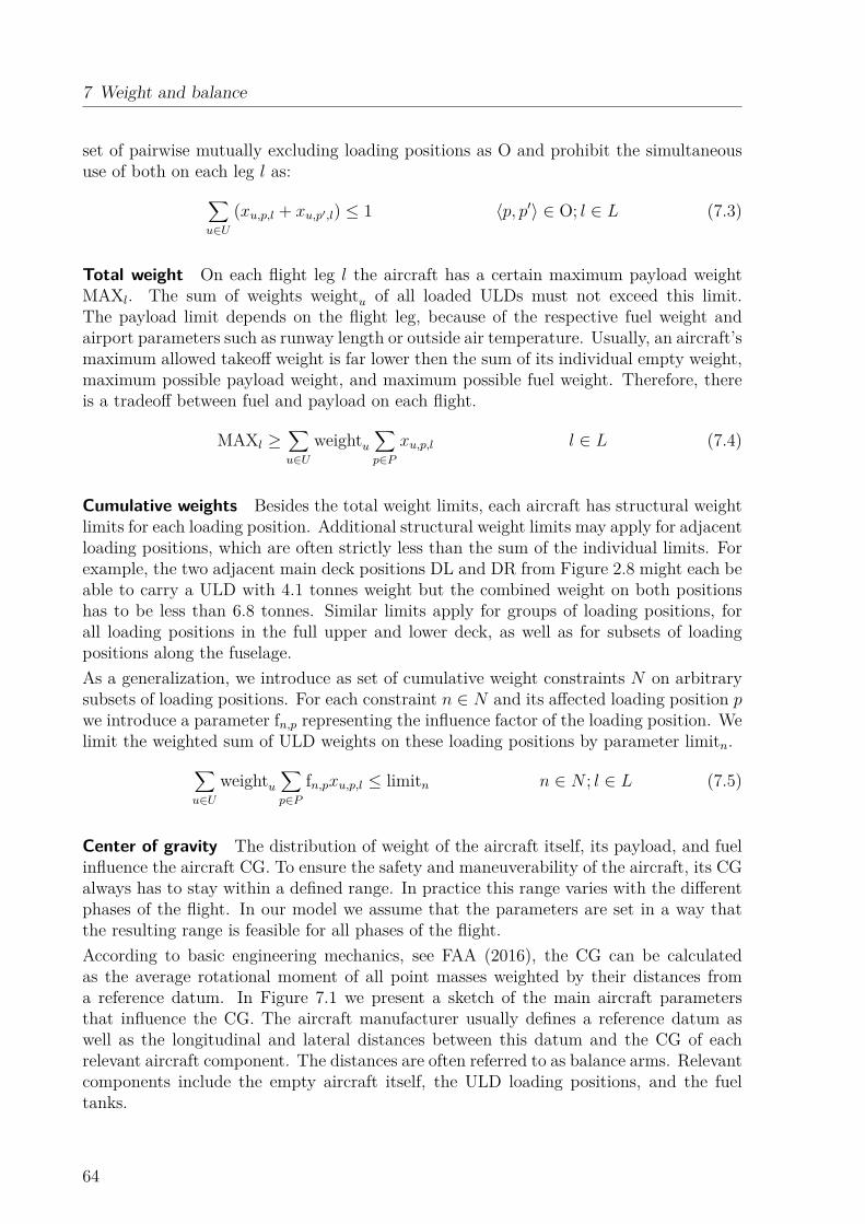
7 Weight and balance
set of pairwise mutually excluding loading positions as O and prohibit the simultaneoususe of both on each leg l as:∑
u∈U(xu,p,l + xu,p′,l) ≤ 1 〈p, p′〉 ∈ O; l ∈ L (7.3)
Total weight On each flight leg l the aircraft has a certain maximum payload weightMAXl. The sum of weights weightu of all loaded ULDs must not exceed this limit.The payload limit depends on the flight leg, because of the respective fuel weight andairport parameters such as runway length or outside air temperature. Usually, an aircraft’smaximum allowed takeoff weight is far lower then the sum of its individual empty weight,maximum possible payload weight, and maximum possible fuel weight. Therefore, thereis a tradeoff between fuel and payload on each flight.
MAXl ≥∑u∈U
weightu∑p∈P
xu,p,l l ∈ L (7.4)
Cumulative weights Besides the total weight limits, each aircraft has structural weightlimits for each loading position. Additional structural weight limits may apply for adjacentloading positions, which are often strictly less than the sum of the individual limits. Forexample, the two adjacent main deck positions DL and DR from Figure 2.8 might each beable to carry a ULD with 4.1 tonnes weight but the combined weight on both positionshas to be less than 6.8 tonnes. Similar limits apply for groups of loading positions, forall loading positions in the full upper and lower deck, as well as for subsets of loadingpositions along the fuselage.As a generalization, we introduce as set of cumulative weight constraints N on arbitrarysubsets of loading positions. For each constraint n ∈ N and its affected loading position pwe introduce a parameter fn,p representing the influence factor of the loading position. Welimit the weighted sum of ULD weights on these loading positions by parameter limitn.∑
u∈Uweightu
∑p∈P
fn,pxu,p,l ≤ limitn n ∈ N ; l ∈ L (7.5)
Center of gravity The distribution of weight of the aircraft itself, its payload, and fuelinfluence the aircraft CG. To ensure the safety and maneuverability of the aircraft, its CGalways has to stay within a defined range. In practice this range varies with the differentphases of the flight. In our model we assume that the parameters are set in a way thatthe resulting range is feasible for all phases of the flight.According to basic engineering mechanics, see FAA (2016), the CG can be calculatedas the average rotational moment of all point masses weighted by their distances froma reference datum. In Figure 7.1 we present a sketch of the main aircraft parametersthat influence the CG. The aircraft manufacturer usually defines a reference datum aswell as the longitudinal and lateral distances between this datum and the CG of eachrelevant aircraft component. The distances are often referred to as balance arms. Relevantcomponents include the empty aircraft itself, the ULD loading positions, and the fueltanks.
64

7.2 The Weight and Balance Model
lng
BAfuell
BAac
MINCGl
MAXCGl
p
BAlngp
Reference datumFuel tank CGEmpty aircraft CGCenters of loading positionsFeasible overall CG
Figure 7.1: Illustration of the components influencing the longitudinal aircraft CG
The CG has to be considered in longitudinal and lateral dimension. The longitudinalCG influences the pitch of the aircraft, while the lateral CG influences the roll. Asthe longitudinal CG has considerably larger balance arms, it is usually of far greaterimportance than the lateral CG. Therefore, we will always refer to the longitudinal CGin the following, if not stated otherwise.We introduce parameters for the longitudinal balance arms of the empty aircraft BAac,each loading position p as BAlng
p , and the fuel as BAfuell on each leg l. The corresponding
weight parameters are the operating empty weight of the aircraft wOEW, the weight offuel FWl on leg l, and the total weight weightu of ULD u. For each leg l we calculate therotational moment of the loaded aircraft ml as:
ml = BAacwOEW + BAfuell FWl +
∑u∈U
weightu∑p∈P
BAlngp xu,p,l l ∈ L (7.6)
To determine the aircraft CG, we need to set the rotational moment in relation to thetotal weight of the aircraft. We calculate the total weight at the beginning of each leg las:
wl = wOEW + FWl +∑u∈U
weightu∑p∈P
xu,p,l l ∈ L (7.7)
The CG on leg l can now be calculated as ml/wl. On each leg the CG has a forward limitMINCGl and aft limit MAXCGl. To avoid the division of variables we limit the rotationalmoments and not the CG itself:
MINCGlwl ≤ ml ≤ MAXCGlwl l ∈ L (7.8)
The lateral CG of the empty aircraft, the fuel weights, and the optimal lateral CG areusually all at the center of the aircraft. Therefore, we only look at the payload for
65

7 Weight and balance
calculating the lateral CG, or rather the payload imbalance. Let BAlatp denote the lateral
balance arm of loading position p. We introduce the auxiliary variables mlat-l and mlat+
l
indicating a lateral moment to the left or right of the aircraft. We calculate the momentof the lateral imbalance as:∑
p∈Pweightu
∑u∈U
BAlatp xu,p,l = mlat+
l −mlat-l l ∈ L (7.9)
The pilots may be able to adjust small lateral imbalances by pumping fuel between thewing tanks. However, the imbalance should be small to maintain flexibility. Therefore,we limit the imbalance on each leg l to BAMAX
l as:
mlat+l +mlat-
l ≤ BAMAXl wl l ∈ L (7.10)
Moment of inertia Weight limits and an ideal CG are not sufficient to describe a goodloading pattern. As an example, a good CG might be reached by placing one ULD onthe front and one at the back of the aircraft and nothing in between. While this mightbe feasible with respect to weight and CG considerations, it would result in a higher thannecessary MI of the aircraft. With a higher MI the aircraft becomes less maneuverableas more power is needed to raise or lower the aircraft’s pitch. Consequently, we want tominimize the MI by placing heavier ULDs closer to the aircraft CG.To simplify the formulation we use the optimal CG of the aircraft BAOPT
l instead of theactual CG, because the former is a constant while the latter is a decision variable. Thisis reasonable because we expect the actual CG to be close to the optimum as this is partof our objective function.We introduce an auxiliary variable mmi
l to approximate the MI added by the loaded ULDson each leg l as:
mmil =
∑u∈U
weightu∑p∈P
(BAOPTl − BAlng
p )2xu,p,l l ∈ L (7.11)
Loading dependencies In practice a loading position might only be usable, if otherloading positions are also in use. The most common use case is that the loading positionsright after the cockpit should be occupied on flights where ULDs are loaded on the loadingpositions behind them. In case of an accident, the ULDs to the front provide a cushionand reduce the impact of broken loose ULDs from behind, to protect the crew and reducedamage to the aircraft.For each loading position p we introduce a set of loading positions Rp the loadability ofp depends on. On each leg l at least one position of Rp must be occupied to be allowedto use p. ∑
u∈Uxu,p,l ≤
∑p′∈Rp
∑u∈U
xu,p′,l p ∈ P ; l ∈ L (7.12)
ULD separation The same item incompatibility constraints that apply during palletiza-tion also apply during flight. Therefore, two ULDs that contain incompatible items mustbe loaded at positions that are a certain minimum distance apart.
66

7.2 The Weight and Balance Model
We introduce the set S of conflicting ULDs and a parameter minu,u′ representing theminimum required distance between the pairs of ULDs. Furthermore, let distp,p′ denotethe distance in the aircraft between loading positions p and p′. On each leg l we restrictthe applicable loading positions as:
∑p′∈P :
distp,p′<minu,u′
xu,p,l + xu′,p′,l ≤ 1 〈u, u′〉 ∈ S; p ∈ P ; l ∈ L (7.13)
Loading operations Cargo flights often contain multiple legs, at which only a part ofthe ULDs are unloaded and others are loaded. As the loading positions are generallyonly accessible in a first-in-last-out style, the assignment of ULDs to loading positionsinfluences the handling effort at each stop. ULDs can be reloaded between the legs, ifthis is beneficial, i.e., it reduces the fuel consumption, or allows to load more cargo.We consider two types of handling operations in the following: unloading a ULD andloading a ULD. We introduce the auxiliary variable ql,p to indicate if the loading positionp needs to be cleared at the stop after leg l. A position needs to be cleared if a ULD isremoved from this position, a ULD is loaded at the position, or if the position is on thepath Bp of another position that needs to be cleared. For all legs but the last, denotedas L′, we add:
ql,p ≥ xu,p,l − xu,p,l+1 u ∈ U ; p ∈ P ; l ∈ L′ (7.14)ql,p ≥ xu,p,l+1 − xu,p,l u ∈ U ; p ∈ P ; l ∈ L′ (7.15)ql,p ≤ ql,p′ p ∈ P ; p′ ∈ Bp; l ∈ L′ (7.16)ql,p ≤ ql,p′ p ∈ P ; p′ ∈ Bp; l ∈ L′ (7.17)
Furthermore, we add auxiliary variables runl,p and ronl,p to indicate if a real handling operationtakes place. These are set to one if a ULD at this position p is loaded or unloaded at thestop after leg l.
runl,p ≥ ql,p +∑u∈U
xu,p,l − 1 p ∈ P ; l ∈ L (7.18)
ronl,p ≥ ql,p +∑u∈U
xu,p,l+1 − 1 p ∈ P ; l ∈ L (7.19)
To sum up the overall loading effort after leg l we use three variables representing the totalnumber of offloaded ULDs runl , the total number of loaded ULDs ronl , and the distance ofmoving ULDs out of and into the aircraft rdistl .
runl =∑p∈P
runl,p l ∈ L (7.20)
ronl =∑p∈P
ronl,p l ∈ L (7.21)
rdistl =∑p∈P
distp(runl,p + ronl,p) l ∈ L (7.22)
67

7 Weight and balance
7.2.4 Objective
There are four factors that make up a good weight and balance solution. First, all ULDsshould be loaded. Second, the longitudinal deviation from the optimal CG should beminimized. Third, the MI of the payload should be small. And last, there should beas few handling operations as possible at each stop-over airport. In our objective weweight these factors by their induced cost. First, we describe how to determine the costparameters.In some setups it might not be possible to load all ULDs. In these cases the least importantULDs should be left behind. Let aoffu denote the penalty cost of offloading ULD u. Inpractice this can be derived from the items loaded into the ULD and the respectivecontracts with the shippers.As mentioned before, the CG also influences the fuel consumption of the aircraft duringflight. Therefore, we estimate the additional fuel consumption attributed to the deviationfrom the optional CG on each flight leg. Let BAOPT
l denote the optimal point at whichthe aircraft consumes the least fuel on leg l. The variable wl denotes the total weight ofthe aircraft and ml its total rotational moment at the beginning of leg l. Let the variablesmlng-l and mlng+
l denote the absolute deviation from the moment of the optimal CG to thefront and aft. We calculate them as:
BAOPTl wl −ml = mlng+
l −mlng-l ∀l ∈ L (7.23)
To transform this into cost, we add parameter acgl for each leg l representing the additionalfuel cost for each unit the moment deviates from the optimum. This cost factor mostlydepends on the aircraft type, the expected flight duration and the fuel price.Nearly the same applies to the MI. A higher MI increases the necessary force to change theaircraft’s direction of flight. This leads to higher drag and additional fuel consumption.To transform the MI into cost, we weight it by a parameter ami
l for each leg l.To determine the cost of loading operations, we introduce parameters that representthe cost at the destination airport of leg l for one unloading operation aunl , one loadingoperation aonl , and the cost of working time when moving a ULD by one loading positionadistl . These costs are usually well known to the airline and defined in the contracts withthe respective ground handling agents or airports.To sum up, we define the total objective function for the WBM to minimize the sum ofcosts stemming from offload penalties, additional fuel consumption on all flight legs, apenalty for the MI, as well as the handling efforts for ULD unloading, loading, and movingefforts at all visited airports along the flight:
minimize∑u∈U
aoffu xoffu +∑l∈L
acgl (mlng-l +mlng+
l )
+amil m
mil + aunl runl + aonl ronl + adistl rdistl
(7.24)
7.2.5 Model overview
After introducing all components of the WBM in the last sections, we now give a consol-idated view of the full model:
68

7.2 The Weight and Balance Model
minimize∑u∈U
aoffu xoffu +∑l∈L
acgl (mlng-l +mlng+
l )
+amil m
mil + aunl runl + aonl ronl + adistl rdistl
(7.25)
subject to
xoffu = 1−∑
p∈loadableu
xu,p,l u ∈ U ; l ∈ legsu (7.26)
1 ≥∑u∈U
xu,p,l p ∈ P ; l ∈ L (7.27)
1 ≥∑u∈U
(xu,p,l + xu,p′,l) 〈p, p′〉 ∈ O; l ∈ L (7.28)
MAXl ≥∑u∈U
weightu∑p∈P
xu,p,l l ∈ L (7.29)
limitn ≥∑u∈U
weightu∑p∈P
fn,pxu,p,l n ∈ N ; l ∈ L (7.30)
ml = BAacwOEW + BAfuell FWl
+∑u∈U weightu
∑p∈P BAlng
p xu,p,ll ∈ L (7.31)
wl = wOEW + FWl +∑u∈U
weightu∑p∈P
xu,p,l l ∈ L (7.32)
BAOPTl wl = ml +mlng+
l −mlng-l l ∈ L (7.33)
ml ≤ MAXCGlwl l ∈ L (7.34)ml ≥ MINCGlwl l ∈ L (7.35)
mlat+l =
∑p∈P
weightu∑u∈U
BAlatp xu,p,l +mlat-
l l ∈ L (7.36)
BAMAXl wl ≥ mlat+
l +mlat-l l ∈ L (7.37)
mmil =
∑u∈U
weightu∑p∈P
(BAOPTl − BAlng
p )2xu,p,l l ∈ L (7.38)∑u∈U
xu,p,l ≤∑p′∈Rp
∑u∈U
xu,p′,l p ∈ P ; l ∈ L (7.39)
1 ≥∑p′∈P :
distp,p′<minu,u′
xu,p,l + xu′,p′,l 〈u, u′〉 ∈ S; p ∈ P ; l ∈ L (7.40)
ql,p ≥ xu,p,l − xu,p,l+1 u ∈ U ; p ∈ P ; l ∈ L (7.41)ql,p ≥ xu,p,l+1 − xu,p,l u ∈ U ; p ∈ P ; l ∈ L (7.42)ql,p ≤ ql,p′ p ∈ P ; p′ ∈ Bp; l ∈ L (7.43)ql,p ≤ ql,p′ p ∈ P ; p′ ∈ Bp; l ∈ L (7.44)runl,p ≥ ql,p +
∑u∈U
xu,p,l − 1 p ∈ P ; l ∈ L (7.45)
ronl,p ≥ ql,p +∑u∈U
xu,p,l+1 − 1 p ∈ P ; l ∈ L (7.46)
rdistl =∑p∈P
distp(runl,p + ronl,p) l ∈ L (7.47)
69
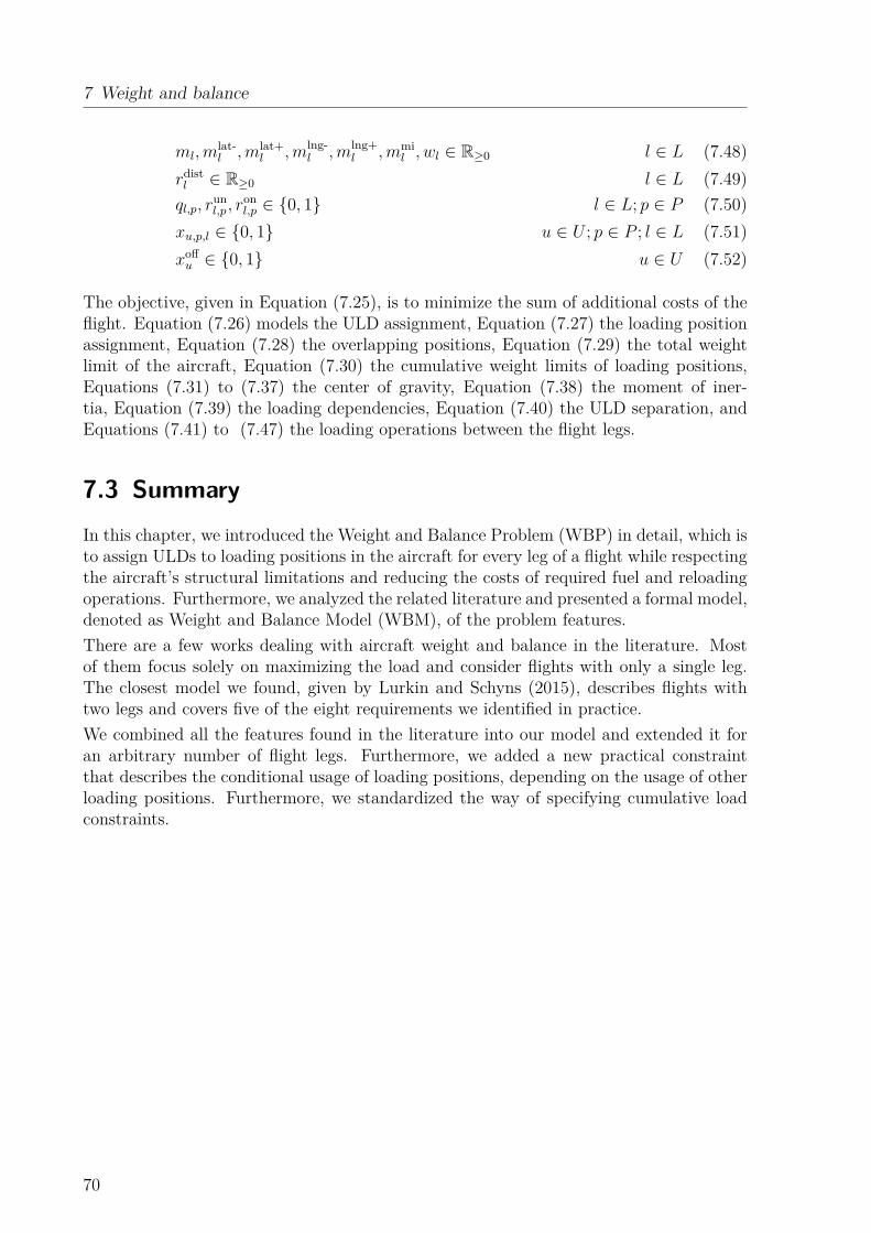
7 Weight and balance
ml,mlat-l ,mlat+
l ,mlng-l ,mlng+
l ,mmil , wl ∈ R≥0 l ∈ L (7.48)
rdistl ∈ R≥0 l ∈ L (7.49)ql,p, r
unl,p , r
onl,p ∈ {0, 1} l ∈ L; p ∈ P (7.50)
xu,p,l ∈ {0, 1} u ∈ U ; p ∈ P ; l ∈ L (7.51)xoffu ∈ {0, 1} u ∈ U (7.52)
The objective, given in Equation (7.25), is to minimize the sum of additional costs of theflight. Equation (7.26) models the ULD assignment, Equation (7.27) the loading positionassignment, Equation (7.28) the overlapping positions, Equation (7.29) the total weightlimit of the aircraft, Equation (7.30) the cumulative weight limits of loading positions,Equations (7.31) to (7.37) the center of gravity, Equation (7.38) the moment of iner-tia, Equation (7.39) the loading dependencies, Equation (7.40) the ULD separation, andEquations (7.41) to (7.47) the loading operations between the flight legs.
7.3 SummaryIn this chapter, we introduced the Weight and Balance Problem (WBP) in detail, which isto assign ULDs to loading positions in the aircraft for every leg of a flight while respectingthe aircraft’s structural limitations and reducing the costs of required fuel and reloadingoperations. Furthermore, we analyzed the related literature and presented a formal model,denoted as Weight and Balance Model (WBM), of the problem features.There are a few works dealing with aircraft weight and balance in the literature. Mostof them focus solely on maximizing the load and consider flights with only a single leg.The closest model we found, given by Lurkin and Schyns (2015), describes flights withtwo legs and covers five of the eight requirements we identified in practice.We combined all the features found in the literature into our model and extended it foran arbitrary number of flight legs. Furthermore, we added a new practical constraintthat describes the conditional usage of loading positions, depending on the usage of otherloading positions. Furthermore, we standardized the way of specifying cumulative loadconstraints.
70

8 Benchmark instancesTo evaluate and compare solution approaches to the ACLPP one needs a set of benchmarkinstances. Unfortunately, there are no suitable instances available yet, neither syntheticones nor instances stemming from practice. We mainly attribute this to the fact thatthe ACLPP has not been considered as a whole in the past. But even in papers dealingwith parts of the problem, like Mongeau and Bes (2003), Rong and Grunow (2009), orLurkin and Schyns (2015), the authors did not publish any of the problem instances theyworked with. From the airline’s point of view, this is comprehensible as booking data areseen as a trade secret. They would allow insights into the airline’s state of business in ahighly competitive market. Furthermore, the concrete shipment data could even allow toidentify the shippers and draw conclusions about their state of business. The same issuesapply in our case. For the development and evaluation of our approach, we work withoriginal datasets provided by our industrial partner, but we cannot publish them.To make our results reproducible, we also create a set of publishable synthetic instances.Simply creating random instances would not be of much use, as the ACLPP exhibitsa lot of structure that can be exploited by a solution approach. Hence, the instancesneed to be carefully designed, to keep a maximum of the typical problem structure of theACLPP in practice. We do this by analyzing the provided real world data, we extracttheir key characteristics and derive new synthetic instances from the given booking datain a suitable way.This chapter is structured as follows. First, we introduce the ACLPP data model inSection 8.1. It combines the models and parameters described in Chapters 4 to 7. After-wards, we present an analysis of the typical properties and problem structure of air cargobookings found at our industrial partner in Section 8.2. We present the actual datasetsused for our evaluation in Section 8.3. Finally, we describe a set of performance indicatorsto compare solutions to the ACLPP and to relate our results to practice in Section 8.4.
8.1 The ACLPP data modelTo describe our data model of the ACLPP, we differentiate three types of relevant in-formation: master data, booking data, and model decisions. In Figure 8.1 we give anoverview of the data model, presenting all entities and their relations.The master data describe all the properties of the aircraft, ULD types, airline objectives,regulatory requirements, terminal workstations, and available workers. We collected andvalidated these data with great effort to evaluate our solution approaches in a realisticsetup. Most of the parameters are similar for many airlines in the industry.The booking data are specific to each flight. All flights together determine the workloadof the air cargo terminal. Each flight’s booking data consists of a list of shipments. A

8 Benchmark instances
Figure 8.1: Data model representing all master data (yellow, green), flight data (red),booking data (violet) and decisions (blue) present in the ACLPP.
72

8.2 Analysis and insights into real world instances
shipment represents a single booking of a shipper with a certain origin, destination, prod-uct, and the expected arrival time at the export terminal. A product defines the servicelevel of the shipment, typically standard or express. Shipments can contain multiple dif-ferent items. Each item type is specified by its dimensions, weight, offload penalty, andhandling requirements. The latter contain information about the allowed item rotations,load-bearing strength, and dangerous goods with their respective net weights. Often, abooking contains multiple items of an item type. Until the airline gets hold of the items,some parameters are still uncertain. The item dimensions and weight might slightlychange and it might turn out that items are not stackable or not rotatable althoughstated differently by the shipper.The model decisions correspond to the subproblems of the ACLPP. They contain theset of used ULDs with their assigned build-up workstation, build-up time, and loadingposition inside the aircraft on each flight leg. For each item of each shipment, the decisionscontain the information if the item is loaded or offloaded and, if loaded, the assigned ULDas well as the placement position and rotation inside the ULD.
8.2 Analysis and insights into real world instancesBefore we introduce our benchmark instances in the next section, we first analyze acollection of real booking data provided by our industrial partner. The main purposeof our analysis is to get an impression of the typical problem structure and the order ofmagnitude of the main parameters.The basis for this analysis is a representative set of booking data of more than 400 flightswith over 35,000 real shipments from the year 2014. The concrete characteristics of thedata will most likely be different for other companies and network structures. An obviousreason is the varying composition of transported commodities between different countriesand continents. The Boeing World Air Cargo Forecast (Crabtree et al., 2014) for examplestates that more than 50 percent of the shipments from Europe to the Americas consist ofchemicals and machinery. On the other hand, shipments from Asia to Europe contain morethan 50 percent computers and apparel. Shipments containing the latter commoditiesare typically lighter, less bulky, and more fragile. Therefore, loading problems betweenAsia and Europe will most likely be of a different nature than between Europe and theAmericas. For further insights into the structure of shipments between different regionsof the world, we refer to the Boeing report mentioned above.We start our analysis by looking at the typical utilization of flights, followed by thestructure of shipments. Afterwards, we investigate the item dimensions, weights, andpresent transfer times in the terminal.
Flight legs A flight might consist of multiple successive legs. The larger the number oflegs the more complex the aircraft configuration and weight and balance decisions, becauseULDs with different origins or destinations must be arranged in the aircraft. Figure 8.2presents the distribution of legs per flight in the typical flight plan of our partner. Lessthan one third of the flights had only one leg. The majority needed to deal with multiplelegs and transport segments.
73
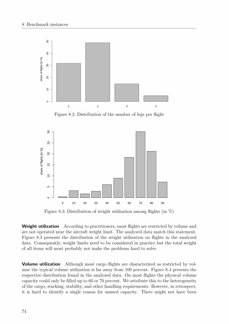
8 Benchmark instances
1 2 3 4
shar
e of
flig
hts
[in %
]
010
2030
4050
Figure 8.2: Distribution of the number of legs per flight
5 15 25 35 45 55 65 75 85 95
weight utilization [in %]
shar
e of
flig
hts
[in %
]
05
1015
2025
30
Figure 8.3: Distribution of weight utilization among flights (in %)
Weight utilization According to practitioners, most flights are restricted by volume andare not operated near the aircraft weight limit. The analyzed data match this statement.Figure 8.3 presents the distribution of the weight utilization on flights in the analyzeddata. Consequently, weight limits need to be considered in practice but the total weightof all items will most probably not make the problems hard to solve.
Volume utilization Although most cargo flights are characterized as restricted by vol-ume the typical volume utilization is far away from 100 percent. Figure 8.4 presents therespective distribution found in the analyzed data. On most flights the physical volumecapacity could only be filled up to 60 or 70 percent. We attribute this to the heterogeneityof the cargo, stacking, stability, and other handling requirements. However, in retrospect,it is hard to identify a single reason for unused capacity. There might not have been
74

8.2 Analysis and insights into real world instances
5 15 25 35 45 55 65 75 85 95
volume utilization [in %]
shar
e of
flig
hts
[in %
]
05
1015
2025
30
Figure 8.4: Distribution of volume utilization on flights (in %)
0 100 300 500 700 900 1100 1300 1500
items per segment
shar
e of
flig
hts
[in %
]
05
1015
20
Figure 8.5: Distribution of the number of items per segment
enough bookings, bookings might have been canceled at short notice, some shipmentsmight have arrived too late, the cargo might have had adverse dimensions or stackingproperties, or it might have been packed in an inefficient way.
Items per segment As packing problems are known to be NP-complete, the numberof items to pack strongly influences the solution complexity. In Figure 8.4 we analyzethe distribution of items per transport segment found in the analyzed data. On average,each segment contained 349 items. Around 3.8 percent of the segments had more than1,000 individual items. The maximum number we found on any segment was close to2,000 items.
75
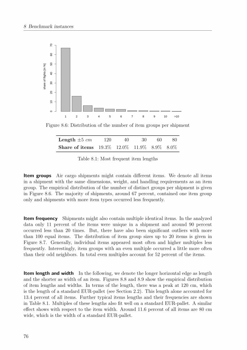
8 Benchmark instances
1 2 3 4 5 6 7 8 9 10 >10
shar
e of
flig
hts
[in %
]
010
2030
4050
6070
Figure 8.6: Distribution of the number of item groups per shipment
Length ±5 cm 120 40 30 60 80Share of items 19.3% 12.0% 11.9% 8.9% 8.0%
Table 8.1: Most frequent item lengths
Item groups Air cargo shipments might contain different items. We denote all itemsin a shipment with the same dimensions, weight, and handling requirements as an itemgroup. The empirical distribution of the number of distinct groups per shipment is givenin Figure 8.6. The majority of shipments, around 67 percent, contained one item grouponly and shipments with more item types occurred less frequently.
Item frequency Shipments might also contain multiple identical items. In the analyzeddata only 11 percent of the items were unique in a shipment and around 90 percentoccurred less than 20 times. But, there have also been significant outliers with morethan 100 equal items. The distribution of item group sizes up to 20 items is given inFigure 8.7. Generally, individual items appeared most often and higher multiples lessfrequently. Interestingly, item groups with an even multiple occurred a little more oftenthan their odd neighbors. In total even multiples account for 52 percent of the items.
Item length and width In the following, we denote the longer horizontal edge as lengthand the shorter as width of an item. Figures 8.8 and 8.9 show the empirical distributionof item lengths and widths. In terms of the length, there was a peak at 120 cm, whichis the length of a standard EUR-pallet (see Section 2.2). This length alone accounted for13.4 percent of all items. Further typical items lengths and their frequencies are shownin Table 8.1. Multiples of these lengths also fit well on a standard EUR-pallet. A similareffect shows with respect to the item width. Around 11.6 percent of all items are 80 cmwide, which is the width of a standard EUR-pallet.
76

8.2 Analysis and insights into real world instances
1 2 3 4 5 6 7 8 9 10 11 12 13 14 15 16 17 18 19 20
shar
e of
item
s [in
%]
02
46
810
12
Figure 8.7: Distribution of item frequencies in all shipments (to be read as: around 9 per-cent of all items belong to a group of 2 items)
0 20 40 60 80 100 120 140 160 180 200 220 240 260 280 300
shar
e of
item
s [in
%]
05
1015
20
Figure 8.8: Distribution of item lengths (in cm)
77

8 Benchmark instances
10 30 50 70 90 110 130 150 170 190 >200
shar
e of
item
s [in
%]
05
1015
20
Figure 8.9: Distribution of item widths (in cm)
0 0.1 0.2 0.3 0.4 0.5 0.6 0.7 0.8 0.9 1
shar
e of
item
s [in
%]
05
1015
20
Figure 8.10: Distribution of width-to-length aspect ratio
Aspect ratio We define the aspect ratio by the ratio between the horizontal edges of theitems, i.e., the item width divided by the item length. Figure 8.10 shows the empiricaldistribution of the aspect ratio. The most frequent ratio was 0.667, accounting for morethan 20 percent of all items. Further typical aspect ratios are shown in Table 8.2.Not surprisingly the most frequent item length (120 cm) and width (80 cm) resemble themost frequent aspect ratio (2:3). Around 10 percent of the items had this base size.
Item height Figure 8.11 shows the empirical distribution of the item heights. The mostfrequent heights were 20 cm to 40 cm and the mean height was 57 cm. Comparing thisto a maximum height of up to 300 cm for main deck ULDs, some stacking seems to benecessary, but there will hardly be more than 10 items on top of each other. In theanalyzed dataset, item heights tend to be higher for larger items. Therefore, we alsolook at the length-to-height ratio of the items. Figure 8.12 shows the corresponding
78

8.2 Analysis and insights into real world instances
Ratio 0.667 0.750 1.000 0.833Alias 2:3 3:4 1:1 5:6Share of items 20.1% 14.7% 14.7% 8.9%
Table 8.2: Popular width-to-length aspect ratios of items
0 20 40 60 80 100 120 140 160 180 200 220 240
shar
e of
item
s [in
%]
05
1015
20
Figure 8.11: Distribution of item heights (in cm)
distribution. The most frequent ratio was 1.5, accounting for 8.6 percent of the items.Furthermore, integer multiples occurred a bit more often than the fractional values close-by. However, it is not clear if this is a real effect or just caused by shippers rounding itemdimensions.
Item weight In the analyzed booking data item weight correlates with item volume.Therefore, we consider the item density in the following. The corresponding distribu-tion is shown in Figure 8.13. The most frequent item densities were between 100 and150 kg ·m−3. From Table 2.4 we know that typical cargo aircraft have a capacity ratio ofaround 180 kg ·m−3. Therefore, we expect the loading problems to be more constrainedby volume than by weight and thus the related three-dimensional packing problems arenon-trivial to solve. This observation is in line with our findings regarding the weightutilization above.
Transfer times Each shipment must be handled in the time between its arrival at theairport and the scheduled departure time of its outgoing flight. We denote this interval astransfer time. In general, a shorter transfer time provides less options to combine itemsonto ULDs and thus makes it harder to find good packing solutions. In the following,we analyze the transfer time of shipments that arrived via an inbound flight or RFS. Inour analysis, we omit shipments that started their journey at the terminal due to missingarrival data. According to practitioners, these shipments typically arrive rather late, mostof them less than 12 hours before the flight departure.
79
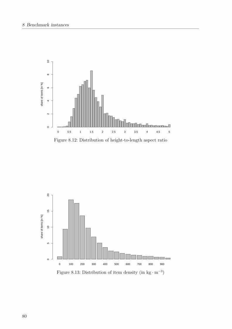
8 Benchmark instances
0 0.5 1 1.5 2 2.5 3 3.5 4 4.5 5
shar
e of
item
s [in
%]
02
46
810
Figure 8.12: Distribution of height-to-length aspect ratio
0 100 200 300 400 500 600 700 800 900
shar
e of
item
s [in
%]
05
1015
20
Figure 8.13: Distribution of item density (in kg ·m−3)
80

8.2 Analysis and insights into real world instances
0−6 6−12 12−18 18−24 24−30 30−36 36−42 42−48 48−54 54−60 60−66 66−72
shar
e of
ava
ilabl
e vo
lum
e [in
%]
020
4060
8010
0
Figure 8.14: Item availability of standard shipments in hours before departure
0−6 6−12 12−18 18−24 24−30 30−36 36−42 42−48 48−54 54−60 60−66 66−72
shar
e of
ava
ilabl
e vo
lum
e [in
%]
020
4060
8010
0
Figure 8.15: Item availability of express shipments in hours before departure
We consider standard and express shipments separately. Express shipments are sold ata premium and allow the shipper to book connections with a shorter transfer time. Forboth product types, the available cargo volume within a certain transfer time is shownin Figures 8.14 and 8.15. As one would expect, express shipments generally exhibit ashorter transfer time than standard shipments. Accordingly, around 42 percent of thestandard volume and 77 percent of the express volume arrives during the last 24 hoursbefore departure.We note that the available time for the actual build-up of the cargo is significantly shorterthan the transfer time. First, the inbound ULDs must be unloaded from the aircraft,transported to the terminal and broken down. The same applies to the aircraft loadingafter the build-up. Accordingly, the handling time window especially for express shipmentscan become really narrow at times.
81

8 Benchmark instances
8.3 Datasets
We present two datasets to evaluate our approach. The first is a set of 89 real historicall-cargo flights (dataset A) provided by our industrial partner. The second set con-tains 82 synthetic flights (dataset B) that we created based on real-world booking data.Dataset B is publicly available under https://github.com/fbrandt/ACLPP. In bothdatasets, the flights add up to a one-week flight schedule. All flights are performed byan MD11F aircraft, whose characteristics we introduced in Section 2.4. Large all-cargoaircraft like the MD11F are the most challenging to plan, because they can load muchmore cargo than smaller or passenger aircraft and a lot more loading constraints mustbe adhered. Accordingly, we expect results to these datasets to be easily transferable toother aircraft types. For evaluation we use the same set of master data for both datasets.
8.3.1 Master data
We created a simplified model of the MD11F aircraft depicted in Figure 2.8. It has53 loading positions and 24 pairs of positions are overlapping. We consider 16 partialweight limits and one net weight constraint. The aircraft can load four different types ofULDs. On the main deck, standard pallets (PMC) and double-sized pallets (PGE) can beloaded. On the lower deck, standard pallets (PMC) and half-size containers (AKE) canbe loaded. Note that the PMC pallets built for the main and lower deck have differentcontours and cannot be loaded into the other deck. All four ULD types have been intro-duced in Section 2.3. Furthermore, we consider the 115 item incompatibility constraintsstemming from the original IATA dangerous goods regulations. We apply two sortingcriteria. The first is to split items of the same shipment across as few ULDs as possible.The second is to avoid mixing standard and express shipments on the same ULD.
8.3.2 Generation of synthetic flights
The basis for dataset B is the pool of real booking data analyzed in Section 8.2. Dataset Ais a one week slice of this pool.The flights of the dataset B are taken from the public flight schedule of Lufthansa CargoAG during calendar week 48 of the year 2015. We selected all flights departing fromFrankfurt Airport that were performed by freighter aircraft.For each flight b in B, we drew a random flight x from the pool that has the same numberof legs. From the flight x we took the total payload and the distribution of payloads amongits transport segments. Then, we iteratively drew random shipments from the flights inthe pool until their sum reached the total payload of flight x. Afterwards, we assignedthe drawn shipments to the transport segments of flight b with the same probability asseen at flight x. Finally, we adjusted the arrival time of the drawn shipments to representthe same transfer time as in their original flight.
82
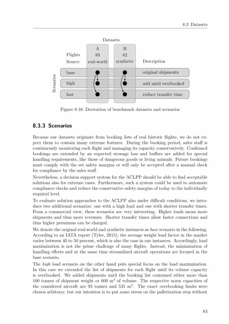
8.3 Datasets
Datasets
Scenarios
DescriptionFlightsSource
A89
real-world
B82
synthetic
base original shipments
high add until overbooked
fast reduce transfer time
Figure 8.16: Derivation of benchmark datasets and scenarios
8.3.3 Scenarios
Because our datasets originate from booking lists of real historic flights, we do not ex-pect them to contain many extreme features. During the booking period, sales staff iscontinuously monitoring each flight and managing its capacity conservatively. Confirmedbookings are extended by an expected stowage loss and buffers are added for specialhandling requirements, like those of dangerous goods or living animals. Future bookingsmust comply with the set safety margins or will only be accepted after a manual checkfor compliance by the sales staff.Nevertheless, a decision support system for the ACLPP should be able to find acceptablesolutions also for extreme cases. Furthermore, such a system could be used to automatecompliance checks and reduce the conservative safety margins of today to the individuallyrequired level.To evaluate solution approaches to the ACLPP also under difficult conditions, we intro-duce two additional scenarios: one with a high load and one with shorter transfer times.From a commercial view, these scenarios are very interesting. Higher loads mean moreshipments and thus more revenues. Shorter transfer times allow faster connections andthus higher premiums can be charged.We denote the original real-world and synthetic instances as base scenario in the following.According to an IATA report (Tyler, 2015), the average weight load factor in the marketvaries between 40 to 50 percent, which is also the case in our instances. Accordingly, loadmaximization is not the prime challenge of many flights. Instead, the minimization ofhandling efforts and at the same time streamlined aircraft operations are focused in thebase scenario.The high load scenario on the other hand puts special focus on the load maximization.In this case we extended the list of shipments for each flight until its volume capacityis overbooked. We added shipments until the booking list contained either more than100 tonnes of shipment weight or 600 m3 of volume. The respective norm capacities ofthe considered aircraft are 93 tonnes and 535 m3. The exact overbooking limits werechosen arbitrary, but our intention is to put some stress on the palletization step without
83
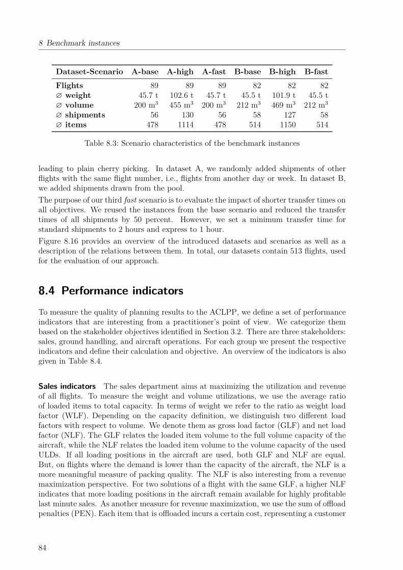
8 Benchmark instances
Dataset-Scenario A-base A-high A-fast B-base B-high B-fastFlights 89 89 89 82 82 82∅ weight 45.7 t 102.6 t 45.7 t 45.5 t 101.9 t 45.5 t∅ volume 200 m3 455 m3 200 m3 212 m3 469 m3 212 m3
∅ shipments 56 130 56 58 127 58∅ items 478 1114 478 514 1150 514
Table 8.3: Scenario characteristics of the benchmark instances
leading to plain cherry picking. In dataset A, we randomly added shipments of otherflights with the same flight number, i.e., flights from another day or week. In dataset B,we added shipments drawn from the pool.The purpose of our third fast scenario is to evaluate the impact of shorter transfer times onall objectives. We reused the instances from the base scenario and reduced the transfertimes of all shipments by 50 percent. However, we set a minimum transfer time forstandard shipments to 2 hours and express to 1 hour.Figure 8.16 provides an overview of the introduced datasets and scenarios as well as adescription of the relations between them. In total, our datasets contain 513 flights, usedfor the evaluation of our approach.
8.4 Performance indicators
To measure the quality of planning results to the ACLPP, we define a set of performanceindicators that are interesting from a practitioner’s point of view. We categorize thembased on the stakeholder objectives identified in Section 3.2. There are three stakeholders:sales, ground handling, and aircraft operations. For each group we present the respectiveindicators and define their calculation and objective. An overview of the indicators is alsogiven in Table 8.4.
Sales indicators The sales department aims at maximizing the utilization and revenueof all flights. To measure the weight and volume utilizations, we use the average ratioof loaded items to total capacity. In terms of weight we refer to the ratio as weight loadfactor (WLF). Depending on the capacity definition, we distinguish two different loadfactors with respect to volume. We denote them as gross load factor (GLF) and net loadfactor (NLF). The GLF relates the loaded item volume to the full volume capacity of theaircraft, while the NLF relates the loaded item volume to the volume capacity of the usedULDs. If all loading positions in the aircraft are used, both GLF and NLF are equal.But, on flights where the demand is lower than the capacity of the aircraft, the NLF is amore meaningful measure of packing quality. The NLF is also interesting from a revenuemaximization perspective. For two solutions of a flight with the same GLF, a higher NLFindicates that more loading positions in the aircraft remain available for highly profitablelast minute sales. As another measure for revenue maximization, we use the sum of offloadpenalties (PEN). Each item that is offloaded incurs a certain cost, representing a customer
84

8.4 Performance indicators
Demand
Shift
Crews
t t+ 1
Demand
Shift
Crews
t t+ 1
Figure 8.17: Sketch of an undesired schedule (left) with peaks and low periods comparedto a desired schedule with even workload (right). Both have the same totalworkload, but the right requires less crews.
refund for late delivery or lost revenue, if an item cannot be transported due to capacityrestrictions. Solutions with a lower PEN are generally preferred by the sales department.
Handling indicators The primary objective of the handling department is to minimizeloading effort, to keep things simple, and to operate with an even workload. To measurehandling effort we introduce four indicators. The first is the total number of used ULDs(UNITS). In a good solution, this should be minimized because each ULD comes with afixed cost as well as the handling effort for preparation and postprocessing. The otherthree indicators relate to item sorting as described in Section 6.2.3. Splitting items thatbelong to the same shipment across multiple ULDs increases the handling effort. For thebuild-up, the shipment needs to be separated and multiple transports to the respectiveworkstations are necessary. This increases the risk that the shipment is partially offloaded.Furthermore, at the next break-down, the items need to be consolidated again. Therefore,we measure the share of splitted shipments (SPLIT) and the average number of differentULDs that the splitted shipments are scattered across (DISP). The last indicator reflectsthe goal that standard and express shipments should not be mixed on the same ULDswhen possible because they will be treated differently at the destination. Therefore,we determine the share of mixed ULDs (MIX) that contain both standard and expressshipments. All sorting indicators should be low in a good solution. To measure theworkload distribution, we introduce a measure for the total number of build-up crewsneeded during all shifts (CREWS). As sketched in Figure 8.17, schedules with an evenworkload during a shift require less crews than schedules containing peak loads and idletimes.
Aircraft operations indicators The aircraft operations department aims at minimizingthe additional fuel consumption, which is induced by aircraft imbalances, and the numberof reloading operations at the stop-over airports. For each type of cost we introduce oneindicator. The extra fuel (FUEL) measures the average cost of kerosene burned, becauseof a suboptimal center of gravity of the aircraft on a flight. The extra loading operations(OPS) measure the cost of unnecessary ULD unloading and loading operations at stop-over airports. We consider a loading operation as unnecessary if a ULD that continues
85

8 Benchmark instances
Name Description Unit ObjectiveWLF avg. weight load factor percent ↗GLF avg. gross load factor percent ↗NLF avg. net load factor percent ↗PEN sum of offload penalty cost ↘UNITS sum of used ULDs #ULDs ↘SPLIT avg. share of split shipments percent ↘DISP avg. split dispersion #ULDs ↘MIX avg. share of mixed ULDs percent ↘CREWS sum of crews in all shifts #crews ↘FUEL sum of extra fuel due to imbalance tonnes ↘OPS sum of unnecessary loading operations #reloads ↘TOTAL sum of total cost of the load plan cost ↘
Table 8.4: Overview of the performance indicators used for evaluation
on the next flight leg needs to be temporarily unloaded or relocated to another loadingposition at a stop-over airport. This might occur because the ULD is blocking anotherULD that needs to be unloaded or to reduce the aircraft’s imbalance on the next flightleg.To combine all the tangible costs of a flight, we further introduce a last indicator of thetotal cost (TOTAL) that combines the penalties of offloaded shipments (PEN), the costof all used ULDs (UNITS), the cost of extra fuel (FUEL), and the cost of unnecessaryloading operations (OPS).
8.5 Summary
In this chapter, we took a look on the data of load planning problems in practice andderived benchmark instances to evaluate our solution approaches.We presented an extensive data model describing the required planning parameters. Onthe one hand, there are a lot of required master data including the aircraft specifications,considered ULD types, workstation setup, regulatory requirements like item incompati-bilities and separation constraints, and commercial objectives. On the other hand, thereare the flight data describing the legs and booked shipments on the respective transportsegments.To get an understanding of the planning challenges, we analyzed a large dataset of realbooking data. We found that flights are often not fully booked. Accordingly, dense packingis not always the prime objective and planning results that lead to efficient handling aswell as aircraft operations are also highly important. Nevertheless, a significant part ofthe items to load is quite large, often exceeding the size of a standard wooden pallet, suchthat finding good three-dimensional packings is non-trivial. Overall, the items to load arestrongly heterogeneous by their dimensions, weight, and density. However, many itemsappear multiple times in a shipment. Furthermore, the planning problems are significantly
86
8.5 Summary
larger than popular benchmark instances for container loading problems. This motivatesthe creation of new benchmark instances of realistic size.From the analyzed booking data, we derived two sets of benchmark instances. Onecontains data of real flights, while the other contains synthesized flights mimicking thereal flights’ properties. The latter dataset is publicly available under https://github.com/fbrandt/ACLPP. For each dataset we created three scenarios to examine interestingvariations from a practical point of view. The first scenario contains just the base data,in the second all flights are overbooked, and in the third scenario the items have shortertransfer times at the terminal. Altogether, we created 513 flights to evaluate our solutionapproaches.In preparation of the evaluation, we discussed suitable performance indicators for loadplanning results from a practical point of view. Fitting to the identified stakeholdersand general objectives, we introduced twelve measures for aircraft utilization, physicalhandling effort, and aircraft operations efficiency.
87


9 A sequential planning approach
In this chapter, we present our first approach to solve the Air Cargo Load Planning Prob-lem (ACLPP). To integrate well with the current manual planning processes of our indus-trial partner introduced in Section 3.3, i.e., the aircraft configuration, build-up scheduling,palletization, and weight and balance, we present a sequential approach that solves thesesteps one by one. The whole process is denoted as SeqACLPP in the following. The maingoal of the SeqACLPP is to automate the manual planning steps of today. Our objectiveis to find a good overall load plan, with respect to all constraints and performance indi-cators presented in Section 8.4. Furthermore, this approach should provide a benchmarkfor process changes.Since the ACLPP cannot be solved independently for each flight and the degree of inter-connection depends on the planning step, we consider three scopes in our solution: theflight plan, flights, and segments. The flight plan usually contains multiple flights, whichcompete for the same resources in the air cargo terminal. A flight potentially consistsof multiple transport segments, which compete for the same resources in the aircraft. InTable 9.1 we give an overview of the planing steps and which scopes are considered in eachindividual run of the respective step. The aircraft configuration is run for each flight. Thebuild-up scheduling is run for the full flight plan at once and considering all the transportsegments. The palletization is run individually for each transport segment. Finally, theweight and balance is solved for each flight.This chapter is organized as follows. In Section 9.1 we present a volume and weightbased approach (VWAC) to solve the Aircraft Configuration Problem (ACP). It decideswhat ULDs should be built for each transport segment of a flight. In Section 9.2 wepresent a rolling horizon planning approach (RHBS) to solve the Build-up SchedulingProblem (BSP). It decides when to build the selected ULDs. After that, we presentour approach to assign and pack items onto the selected and scheduled ULDs (BDAP)by a Logic-based Benders Decomposition (LBBD) solving the Air Cargo Palletization
Problem Aircraft Build-up Air Cargo Weight andConfiguration Scheduling Palletization Balance
Section 9.1 9.2 9.3 9.4Step name VWAC RHBS LBBD UWABFlight plan XFlight X XSegment X X X X
Table 9.1: Entities considered in individual runs of the planning steps
9 A sequential planning approach
Problem (APP). Finally, in Section 9.4 we present our solution step (UWAB) to solve theWeight and Balance Problem (WBP). In this step, the built ULDs are assigned to loadingpositions in the aircraft.
9.1 Volume-and-weight-based aircraft configurationThe first step of our solution approach is to solve the ACP for each flight. In practice,this step is performed multiple times between 24 and 72 hours before a flight. In the earlyruns, not all bookings have arrived and some bookings might still contain placeholders orunconfirmed item data. But, the state of the data continually improves until departure.Accordingly, in the beginning the primary purpose of aircraft configuration is to estimatefuture build-up demands for scheduling build-up workers and ULD provisioning. Only atlater iterations the selected ULDs become more important for palletization preparations.To keep things simple and the amount of required data low, we operate only on sums ofthe booked cargo weight and volume of each transport segment during this step. Giventhe total cargo volume and weight of each transport segment, the aircraft characteristics,and the available ULD types we decide how many ULDs of each type should be built foreach transport segment. We denote this step as VWAC in the following. In the remainderof this section, we introduce some necessary preprocessing steps followed by a descriptionof the employed MIP model.
9.1.1 Preprocessing
The booking data introduced in Section 8.1 contain all the information about the individ-ual shipments. But, as our model operates on aggregated data of each transport segment,we need to derive some model parameters from the input booking data.
Offload penalties Each item to load has a specific penalty offloadi that applies if it isoffloaded. This penalty indicates the lost profit or the refund to the customer. Duringaircraft configuration we only consider the total demand with respect to volume andweight for each transport segment, not the individual items. To do that, we need toderive suitable offload penalties for each segment. In our preprocessing we determine thepenalties as the average penalty across all items Ik on the segment k, weighted by theitem weight and volume respectively:
offloadvolk =
∑i∈Ik
offloadi∑i∈Ik
volumeioffloadwgtk =
∑i∈Ik
offloadi∑i∈Ik
weightgrsik ∈ K (9.1)
Estimated bin capacity In practice it is unlikely that we are able to fill a ULD up toits physical volume capacity. Often the combinatorics between the items and the curvedshape of the ULD will result in some unused space. Therefore, in the following we usethe average achievable volume utilization of each ULD type instead of the real geometric
90

9.1 Volume-and-weight-based aircraft configuration
volume capacity. In practice this utilization can be derived from the built ULDs seen onhistoric flights or earlier iterations of this solution process. We will discuss the impact ofthe estimated capacity on the constructed solutions and the choice of suitable parametersin Section 10.2.1.
Minimum number of required bins The third preprocessing step is to determine theminimum number of ULDs required for certain ULD types. Here, we check for each itemif it would fit into each ULD type. For example, very long items might only fit into PGEULDs and high items that are not rotatable must be placed into the upper deck, thusrequiring a main deck PMC ULD. See Figure 2.3 for an overview of the used ULD types.The geometric volumes of items requiring a special ULD type are summed up and dividedby the average achievable volume utilization for this ULD type. Rounding the result upto the next integer gives us the minimum required number of ULDs of each type.
9.1.2 Mixed-integer model
We solve the aircraft configuration by applying the full Aircraft Configuration Model (ACM)as presented in Section 4.2.5. Table 9.2 recaps the sets and parameters of the model andTable 9.3 presents its decision variables. The model primarily decides about the numberxk,v of ULDs to build for each transport segment k and ULD type v. For completeness,we repeat the ACM with minor adjustments for this step:
minimize∑k∈K
(∑v∈V
xk,vcostv + 12y
wgtk offloadwgtk + 1
2yvolk offloadvolk
)(9.2)
subject to
demwgtk ≤
∑v∈V
xk,vcapwgtv + ywgtk k ∈ K (9.3)
demvolk ≤
∑v∈V
xk,vcapvolv + yvolk k ∈ K (9.4)
limitf ≥∑
k∈K:l∈onk
∑v∈V
mf,vxk,v + (bl,f − 1)M l ∈ L; f ∈ F (9.5)
1 ≤∑f∈G
bl,f l ∈ L;G ∈ F (9.6)
mink,v ≤ xk,v k ∈ K; v ∈ V (9.7)availl,v ≥
∑k∈K:k∈startl
xk,v l ∈ L; v ∈ V (9.8)
bl,f ∈ {0, 1} l ∈ L;G ∈ F (9.9)ywgtk , yvolk ∈ R≥0 k ∈ K (9.10)xk,v ∈ N k ∈ K; v ∈ V (9.11)
The objective, given in Equation (9.2), is to minimize the total cost from the used ULDsand offloaded cargo. Because offloaded items will appear twice, as offloaded volume and
91
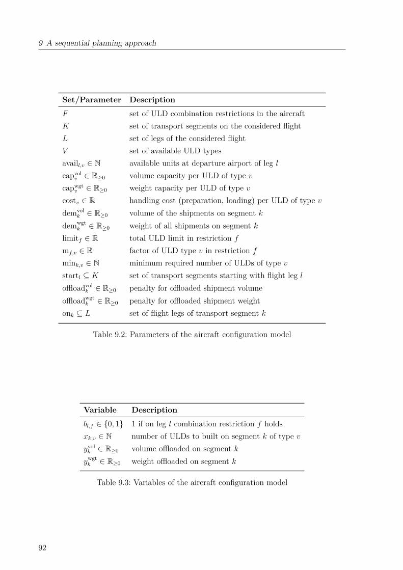
9 A sequential planning approach
Set/Parameter DescriptionF set of ULD combination restrictions in the aircraftK set of transport segments on the considered flightL set of legs of the considered flightV set of available ULD typesavaill,v ∈ N available units at departure airport of leg lcapvolv ∈ R≥0 volume capacity per ULD of type vcapwgtv ∈ R≥0 weight capacity per ULD of type vcostv ∈ R handling cost (preparation, loading) per ULD of type vdemvol
k ∈ R≥0 volume of the shipments on segment kdemwgt
k ∈ R≥0 weight of all shipments on segment klimitf ∈ R total ULD limit in restriction fmf,v ∈ R factor of ULD type v in restriction fmink,v ∈ N minimum required number of ULDs of type vstartl ⊆ K set of transport segments starting with flight leg loffloadvolk ∈ R≥0 penalty for offloaded shipment volumeoffloadwgtk ∈ R≥0 penalty for offloaded shipment weightonk ⊆ L set of flight legs of transport segment k
Table 9.2: Parameters of the aircraft configuration model
Variable Descriptionbl,f ∈ {0, 1} 1 if on leg l combination restriction f holdsxk,v ∈ N number of ULDs to built on segment k of type vyvolk ∈ R≥0 volume offloaded on segment kywgtk ∈ R≥0 weight offloaded on segment k
Table 9.3: Variables of the aircraft configuration model
92
9.2 Rolling horizon build-up scheduling
weight, we multiply the penalties by 12 . In the following we briefly describe the restrictions.
A detailed explanation of the constraints is given in Section 4.2.3.Equations (9.3) and (9.4) make sure that enough weight and volume capacity is reservedor that the cargo is marked as offloaded. Equations (9.5) and (9.6) limit the selected setof ULDs to a valid aircraft configuration. The minimum number of required ULDs pertype on each transport segment are modeled with Equation (9.7). Finally, Equation (9.8)ensures that no more than the available number of ULDs are used at each airport.For simplicity we assume that the handling cost and available ULD types are the same forall visited airports. We note that the model can be easily extended to support differentparameters for each airport.
9.2 Rolling horizon build-up scheduling
All flights departing during the same period compete for the same build-up resources in theair cargo terminal, namely workstations and workers. With a given aircraft configurationfor each flight, we know the number of each ULD type that must be built before eachflight’s departure time. Because only physically available cargo can be loaded into a ULDand each flight has its individual departure time, we need to schedule the ULD build-ups.Furthermore, the schedule must be feasible with respect to the available workstations andworkers.In practice build-up scheduling is a continuous planning process. New jobs to build ULDsfor upcoming flights appear constantly, while the previous flights are already partially builtand ULDs currently in production cannot be changed anymore. To manage this ongoingprocess, we present a planning model with a rolling horizon. We cut the continuous timeinto discrete planning horizons, the build-up crew shifts, and plan each shift after another.We denote this step as RHBS in the following.The remainder of this section is structured as follows. In Section 9.2.1 we introduce somenecessary preprocessing steps to determine suitable parameters for the planning modelsfrom the given flights. Afterwards, we present our MIP model to schedule the build-updemand for a limited time horizon in Section 9.2.2. How this model is used for continuousplanning with a rolling horizon is described in Section 9.2.3.
9.2.1 Preprocessing
Most parameters of the BSP are defined in the booking lists of the flights or are determinedduring the aircraft configuration, see Table 9.3. In this section, we discuss how theremaining parameters, see Section 5.2.1, can be derived from these input data.
Offload penalties Each item to load has a specific offload penalty offloadi. This penaltyindicates the lost profit or the refund to the customer. Due to workstation or workercapacity restrictions we might not be able to schedule all ULDs or we have to schedulethem too early, at a period where not enough cargo is available. In both cases we loosevolume capacity and will have to offload items later. Analog to the offload penalties in
93
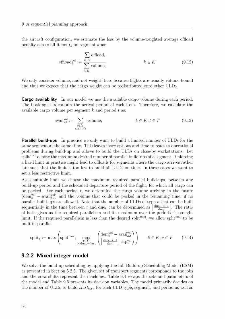
9 A sequential planning approach
the aircraft configuration, we estimate the loss by the volume-weighted average offloadpenalty across all items Ik on segment k as:
offloadvolk :=
∑i∈Ik
offloadi∑i∈Ik
volumeik ∈ K (9.12)
We only consider volume, and not weight, here because flights are usually volume-boundand thus we expect that the cargo weight can be redistributed onto other ULDs.
Cargo availability In our model we use the available cargo volume during each period.The booking lists contain the arrival period of each item. Therefore, we calculate theavailable cargo volume per segment k and period t as:
availvolk,t :=∑i∈Ik:
availi≤t
volumei k ∈ K; t ∈ T (9.13)
Parallel build-ups In practice we only want to build a limited number of ULDs for thesame segment at the same time. This leaves more options and time to react to operationalproblems during build-up and allows to build the ULDs on close-by workstations. Letsplitmax denote the maximum desired number of parallel build-ups of a segment. Enforcinga hard limit in practice might lead to offloads for segments where the cargo arrives ratherlate such that the limit is too low to build all ULDs on time. In these cases we want toset a less restrictive limit.As a suitable limit we choose the maximum required parallel build-ups, between anybuild-up period and the scheduled departure period of the flight, for which all cargo canbe packed. For each period t, we determine the cargo volume arriving in the future(demvol
k − availvolk,t) and the volume that could be packed in the remaining time, if noparallel build-ups are allowed. Note that the number of ULDs of type v that can be builtsequentially in the time between t and duek can be determined as
⌊duek−t−1
durv
⌋. The ratio
of both gives us the required parallelism and its maximum over the periods the soughtlimit. If the required parallelism is less than the desired splitmax, we allow splitmax to bebuilt in parallel.
splitk := maxsplitmax; max
t∈T :t<duek−durv
demvolk − availvolk,t⌊
duek−t−1durv
⌋capvolv
k ∈ K; v ∈ V (9.14)
9.2.2 Mixed-integer model
We solve the build-up scheduling by applying the full Build-up Scheduling Model (BSM)as presented in Section 5.2.5. The given set of transport segments corresponds to the jobsand the crew shifts represent the machines. Table 9.4 recaps the sets and parameters ofthe model and Table 9.5 presents its decision variables. The model primarily decides onthe number of ULDs to build startk,v,t for each ULD type, segment, and period as well as
94

9.2 Rolling horizon build-up scheduling
Set/Parameter DescriptionK set of transport segments to build ULDs forS set of crew shiftsT set of time periodsV set of available ULD typesavailvolk,t ∈ R≥0 demand volume for segment k available at period tcapvolv ∈ R≥0 volume capacity per ULD of type vcosts ∈ R≥0 cost of one build-up crew in shift sdemvol
k ∈ R≥0 total volume of the shipments on segment kduek ∈ T build-up due date of segment kdurv ∈ N number of periods to build-up a ULD of type vends ∈ T last period after shift smaxs ∈ N max build-up crews in shift soffloadvolk ∈ R≥0 offload penalty per volume unit for segment kopenv,t ∈ N open workstations for ULD type v at period tpackk ∈ R≥0 already packed demand volume for segment k at period 0splitk ∈ N max simultaneous build-ups for segment kstarts ∈ T first period of shift suldk,v ∈ N number of ULDs of type v to schedule for segment kδ(v, t) ⊆ T periods when build-ups in progress during period t pot. started
δ(v, t) = {t′ | t′ ∈ T : t− durv < t′ ≤ t}φ(k) ⊆ T periods when ULD build-ups for segment k can be started
φ(k) = {t | t ∈ T : 0 < t ≤ duek}θ(s) ⊆ T periods when workers of shift s can perform build-ups
θ(s) = {t | t ∈ T : starts ≤ t < ends}
Table 9.4: Parameters of the build-up scheduling model
the number of required crews crewss during each shift. Furthermore, it tracks the alreadybuilt volume packk,t for each segment and period. By comparing this with the availablecargo volume in each period, we can derive the lost space inside planned ULDs deadk,tand if necessary the not scheduled ULDs offloadk,v. For completeness, we repeat the BSMwith minor adjustments for this step:
minimize∑k∈K
offloadvolk
(∑t∈T
deadk,t +∑v∈V
capvolv offloadk,v)
+∑s∈S
costscrewss (9.15)
95

9 A sequential planning approach
Variable Descriptioncrewss ∈ N number of crews required during shift sdeadk,t ∈ R≥0 unusable volume capacity during build-ups for segment k in period toffloadk,v ∈ N number of selected but not scheduled ULDs for segment k of type vpackk,t ∈ R≥0 already packed demand volume for segment k prior to period tstartk,v,t ∈ N number of ULDs build-ups started for segment k of type v at period t
Table 9.5: Variables of the build-up scheduling model
subject to
uldk,v = offloadk,v +∑t∈T :
t≤duek−durv
startk,v,t k ∈ K; v ∈ V (9.16)
packk,0 = packk (9.17)packk,t + deadk,t = packk,t−1 +
∑v∈V
startk,v,tcapvolv k ∈ K; t ∈ φ(k) (9.18)
availk,t ≥ packk,t k ∈ K; t ∈ T (9.19)splitk ≥
∑v∈V
∑t′∈δ(v,t)
startk,v,t′ k ∈ K; t ∈ T (9.20)
openv,t ≥∑k∈K
∑t′∈δ(v,t)
startk,v,t′ v ∈ V ; t ∈ T (9.21)∑s∈S:t∈θ(s)
crewss ≥∑k∈K
∑v∈V
∑t′∈δ(v,t)
startk,v,t t ∈ T (9.22)
crewss ∈ N s ∈ S (9.23)deadk,t ∈ R≥0 k ∈ K; t ∈ φ(k) (9.24)offloadk,v ∈ N k ∈ K; v ∈ V (9.25)packk,t ∈ R≥0 k ∈ K; t ∈ φ(k) (9.26)startk,v,t ∈ N k ∈ K; v ∈ V ; t ∈ φ(k) (9.27)
The objective, given in Equation (9.15), is to minimize the sum of the cost of the lostprofit due to early build-ups or unscheduled ULDs and the cost of the deployed crews. Inthe following we briefly describe the restrictions. A detailed explanation of the constraintsis given in Section 5.2.3.Equation (9.16) makes sure that all requested ULDs are built on time or are marked asoffload. Equations (9.17) and (9.18) calculate the already built cargo volume at eachperiod and Equation (9.19) enforces that during each period not more than the alreadyavailable cargo is packed. The number of parallel build-ups for a segment is limited withEquation (9.20). Similar checks make sure that the number of available workstations isrespected in Equation (9.21) and that during each period enough crews are on duty inEquation (9.22).
96
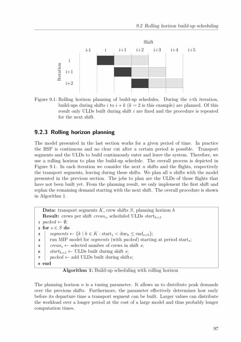
9.2 Rolling horizon build-up scheduling
Shift
Iteration
i-1 i i+1 i+2 i+3 i+4 i+5
i
i+1
i+2
Figure 9.1: Rolling horizon planning of build-up schedules. During the i-th iteration,build-ups during shifts i to i+ k (k = 2 is this example) are planned. Of thisresult only ULDs built during shift i are fixed and the procedure is repeatedfor the next shift.
9.2.3 Rolling horizon planning
The model presented in the last section works for a given period of time. In practicethe BSP is continuous and no clear cut after a certain period is possible. Transportsegments and the ULDs to build continuously enter and leave the system. Therefore, weuse a rolling horizon to plan the build-up schedule. The overall process is depicted inFigure 9.1. In each iteration we consider the next n shifts and the flights, respectivelythe transport segments, leaving during these shifts. We plan all n shifts with the modelpresented in the previous section. The jobs to plan are the ULDs of those flights thathave not been built yet. From the planning result, we only implement the first shift andreplan the remaining demand starting with the next shift. The overall procedure is shownin Algorithm 1.
Data: transport segments K, crew shifts S, planning horizon hResult: crews per shift crewss, scheduled ULDs startk,v,t
1 packed ← ∅;2 for s ∈ S do3 segments ← {k | k ∈ K : starts < duek ≤ ends+h};4 run MIP model for segments (with packed) starting at period starts;5 crewss ← selected number of crews in shift s;6 startk,v,t ← ULDs built during shift s;7 packed ← add ULDs built during shifts;8 end
Algorithm 1: Build-up scheduling with rolling horizon
The planning horizon n is a tuning parameter. It allows us to distribute peak demandsover the previous shifts. Furthermore, the parameter effectively determines how earlybefore its departure time a transport segment can be built. Larger values can distributethe workload over a longer period at the cost of a large model and thus probably longercomputation times.
97
9 A sequential planning approach
9.3 Air cargo palletization
In this section, we present our solution approach to the Air Cargo Palletization Prob-lem (APP). The APP decides which items are placed into which ULD and how they haveto be arranged in the three-dimensional space to fulfill all physical, regulatory, and orga-nizational constraints. In the earlier steps we already selected a suitable superset of ULDsfor each transport segment and assigned a build-up period for each ULD. It is possibleto solve the APP for each transport segment independently, because items for differentsegments must be placed in different ULDs. Therefore, we only consider problems with asingle transport segment in the following.As the three-dimensional packing problem is NP-complete and large real world instancesare typically computationally very hard to solve, we decompose the problem and solveit heuristically. Our approach is known as Logic-based Benders Decomposition (LBBD),which was introduced by Hooker (2007). Its basic idea is to split an optimization probleminto a linear master problem and an arbitrary subproblem. For a given solution to themaster, the subproblem is solved heuristically. If the subproblem turns out to be infeasible,problem-specific heuristic cuts are derived from the subproblem and added to the master.Then the master is solved again and the process is repeated until the subproblem can besolved.In our case, the master problem is a vector container loading problem, denoted as BinAs-sign in the following. It decides, which ULDs to use and how to assign items to them.In the master problem all non-geometric constraints are handled. Our subproblem is athree-dimensional knapsack problem, denoted as CPPack in the following. It needs to besolved for each individual ULD and deals with all the geometric and physical aspects ofthe placement of items inside the ULD. For cases, in which not all boxes can be packedin the subproblem, we derive valid inequalities from the packable subset of items and addthem to the master problem before resolving it. We repeat this process until all ULDscan be successfully packed in the subproblem. On top of the LBBD, we reduce the searchspace heuristically to make the problem solvable within an acceptable time limit. Wedenote this process as BDAP in the following.Our approach implements all but two features of the APP introduced in Section 6.2. Weonly omit item spacing restrictions between ULDs and item positioning restrictions withinthe aircraft, because the ULDs do not have an assigned loading position yet and thus noabsolute coordinates within the aircraft are given. Nevertheless, both restrictions will bemodeled and thus be respected as ULD spacing constraints in the final weight and balancestep. We give an overview which constraints are handled by which part of our solution inTable 9.6.The remainder of this section is structured as follows. In Section 9.3.1 we introducethe MIP formulation of the BinAssign master problem. In Section 9.3.2 we present theconstraint program of the CPPack subproblem. In Section 9.3.3 we describe the cutgeneration and LBBD. Afterwards, we present two methods to reduce the search spaceand to speed up our approach. In Sections 9.3.4 we introduce a decomposition by itemvolume and in Section 9.3.5 the estimation of stowage loss for the items. At last, we recapthe overall procedure in Section 9.3.6.
98
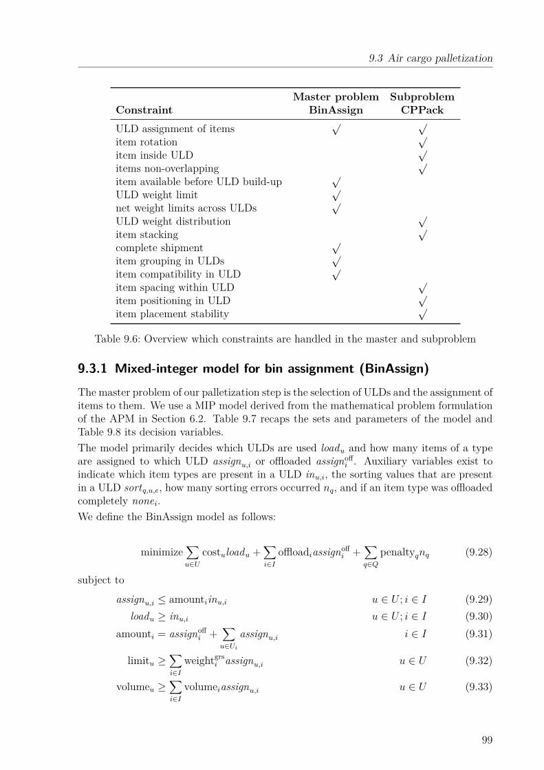
9.3 Air cargo palletization
Master problem SubproblemConstraint BinAssign CPPackULD assignment of items
√ √
item rotation√
item inside ULD√
items non-overlapping√
item available before ULD build-up√
ULD weight limit√
net weight limits across ULDs√
ULD weight distribution√
item stacking√
complete shipment√
item grouping in ULDs√
item compatibility in ULD√
item spacing within ULD√
item positioning in ULD√
item placement stability√
Table 9.6: Overview which constraints are handled in the master and subproblem
9.3.1 Mixed-integer model for bin assignment (BinAssign)
The master problem of our palletization step is the selection of ULDs and the assignment ofitems to them. We use a MIP model derived from the mathematical problem formulationof the APM in Section 6.2. Table 9.7 recaps the sets and parameters of the model andTable 9.8 its decision variables.The model primarily decides which ULDs are used loadu and how many items of a typeare assigned to which ULD assignu,i or offloaded assignoff
i . Auxiliary variables exist toindicate which item types are present in a ULD inu,i, the sorting values that are presentin a ULD sortq,u,e, how many sorting errors occurred nq, and if an item type was offloadedcompletely nonei.We define the BinAssign model as follows:
minimize∑u∈U
costuloadu +∑i∈I
offloadiassignoffi +
∑q∈Q
penaltyqnq (9.28)
subject to
assignu,i ≤ amountiinu,i u ∈ U ; i ∈ I (9.29)loadu ≥ inu,i u ∈ U ; i ∈ I (9.30)
amounti = assignoffi +
∑u∈Ui
assignu,i i ∈ I (9.31)
limitu ≥∑i∈I
weightgrsi assignu,i u ∈ U (9.32)
volumeu ≥∑i∈I
volumeiassignu,i u ∈ U (9.33)
99

9 A sequential planning approach
Set/Parameter DescriptionDg set of net weight limits applying to subsets of ULDs (d ∈ Dg)G set of considered net weight categories (g ∈ G)I set of item types to load (i ∈ I)Q set of sorting criteria (q ∈ Q)Qq value domain of sorting criterion qU set of available ULDs (u ∈ U)A ⊆ I × I pairs of item types not allowed within one ULD (〈i, j〉 ∈ A)amounti number of items of type icliquei ∈ I item type that must be loaded completely to also load type icostu ∈ R≥0 cost when using ULD u
limitnetd ∈ R≥0 net weight limit for all items placed in uldsd for weight limit dlimitu ∈ R≥0 gross weight limit of ULD u
offloadi ∈ R≥0 penalty for each item of type i that is offloadedpenaltyq ∈ R≥0 linear penalty for sorting errors of criterion qpowq ∈ N exponential penalty for sorting errors of criterion qsortq,i ∈ Qq group of item type i w.r.t. sorting criterion qQitem ⊆ Q set of sorting criteria to group items byQuld ⊆ Q set of sorting criteria to separate items byUi ⊆ U ULDs that item type i can be packed intouldsd ⊆ U ULDs considered for net weight limit dvolumei ∈ R≥0 volume of each item of type ivolumeu ∈ R≥0 maximum usable volume of ULD u
weightgrsi ∈ R≥0 gross weight of each item of type iweightnetg,i ∈ R≥0 weight of each item of type i w.r.t. weight category g
Table 9.7: Parameters of the BinAssign model
100

9.3 Air cargo palletization
Variable Descriptionassignu,i ∈ N number of items of type i loaded into ULD u
assignoffi ∈ N number of items of type i that are offloaded
inu,i ∈ {0, 1} is item i present in ULD u
loadu ∈ {0, 1} 1 if ULD u is loadednq ∈ N number of penalties w.r.t. sorting criterion qnonei ∈ {0, 1} 1 if item i is completely loadedsortq,u,e ∈ {0, 1} 1 if sorting value nq is present in ULD u
Table 9.8: Decision variables of the BinAssign model
limitnetd ≥∑
u∈uldsd
∑i∈I
weightnetg,i assignu,i g ∈ G; d ∈ Dg (9.34)
assignoffi = amountinonei i ∈ I (9.35)
nonei = nonecliqueii ∈ I (9.36)
inu,i ≤ sortq,u,sortq,iq ∈ Q;u ∈ U ; i ∈ I (9.37)
nq =∑e∈Qq
(∑u∈U
sortq,u,e)powq
q ∈ Qitem (9.38)
nq =∑u∈U
∑e∈Qq
sortq,u,e
powq
q ∈ Quld (9.39)
1 ≥ inu,i + inu,j u ∈ U ; 〈i, j〉 ∈ A (9.40)assignu,i ∈ N i ∈ I;u ∈ Ui (9.41)assignoff
i ∈ N i ∈ I (9.42)nonei ∈ {0, 1} i ∈ I (9.43)nq ∈ N q ∈ Q (9.44)inu,i ∈ {0, 1} i ∈ I;u ∈ Ui (9.45)loadu ∈ {0, 1} u ∈ U (9.46)sortq,u,e ∈ {0, 1} q ∈ Q;u ∈ U ; e ∈ Qq (9.47)
The objective, given in Equation (9.28), is to minimize the sum of cost of the used ULDs,the penalties of offloaded items, and the penalties for violating the sorting constraints. Inthe following we briefly describe the restrictions. A detailed explanation of the constraintsis given in Section 6.2.3.Equation (9.29) tracks what item types are present in a ULD. According to Equa-tion (9.30) items can only be assigned to a loaded ULD. Equation (9.31) models theassignment of items to ULDs. Equations (9.32) and (9.33) ensure that the ULD’s weightand volume capacity is respected. Complete shipment constraints are enforced by Equa-tions (9.35) and (9.36). Equations (9.37) to (9.39) calculate the penalties with respect tothe different item and bin sorting criteria. Finally, Equation (9.40) models incompatibilityconstraints between items that must not be placed in the same ULD.
101

9 A sequential planning approach
Set/Parameter DescriptionCu set of contour planes of ULD u (〈x, y, z, a〉 ∈ Cu)I the items to pack (i ∈ I)dimx
i , dimyi , dimz
i ∈ R≥0 dimensions of item i
disti,j ∈ R≥0 minimum required distance between items i and joffloadi ∈ R≥0 penalty when item i is offloadedroti ⊆ R allowed rotations of item i
rotationsi ⊆ R4≥0 rotated dimensions and load-bearing strength of item i
stackxi , stackyi , stackzi ∈ R≥0 maximum load-bearing strength of item i
startxu, startyu, startzu ∈ R start coordinate of ULD u
suppi ∈ R≥0 minimum supported area of item i (ratio)udimz
u, udimyu, udimx
u ∈ R≥0 dimensions of ULD u
weightgrsi ∈ R≥0 gross weight of item i
(xcgu , ycgu , zcgu ) ∈ R3 lower bound of the valid CG of ULD u
(xcgu , ycgu , zcgu ) ∈ R3 upper bound of the valid CG of ULD u
( x←−uldu,i , y←−
uldu,i , z←−
uldu,i ) ∈ R3 lower bound of item i start position inside ULD u
(←−x uldu,i ,←−y uld
u,i ,←−z uld
u,i ) ∈ R3 upper bound of item i start position inside ULD u
( x−→uldu,i , y−→
uldu,i , z−→
uldu,i ) ∈ R3 lower bound of item i end position in ULD u
(−→x uldu,i ,−→y uld
u,i ,−→z uld
u,i ) ∈ R3 upper bound of item i end position in ULD u
ε packing height tolerance
Table 9.9: Parameters of the CPPack model for ULD u
9.3.2 Constraint program for the 3D knapsack problem (CPPack)
In the master problem we assigned items to bins with respect to the total volume, weight,and further domain specific constraints. In this section, we present a constraint program-ming model to determine the three-dimensional positions of the items inside the bin withrespect to the geometric and physical constraints. The model considers only one bin, i.e.,it must be run for each bin from the solution of the master problem. We derive our modelfrom the mathematical formulation of the APM in Section 6.2.Table 9.9 introduces the sets and parameters of the model and Table 9.10 presents itsdecision variables. The model decides which of the items assigned to the bin are actuallypacked packi, at which position (xi, yi, zi), and orientation (sizexi , sizeyi , sizezi ). Auxiliaryvariables track the mechanical relations, like the actual load-bearing strength of the itemstacki, how much an item weighs including items stacked on top of it wi, if an item isplaced on the floor floor i, or if it supports another item basei,j. For the calculation ofthe contact areas between two items we track the overlap along the x-axis oxi,j and z-axisozi,j as well as the total supported area of an item oi. Finally, to limit the bin’s center of
102

9.3 Air cargo palletization
Name Min Max Descriptionbasei,j 0 1 1 if item i supports item j
floor i 0 1 1 if item i is placed on the ULD floormx −∞ ∞ moment of packed items on x-axis (2×)my −∞ ∞ moment of packed items on y-axis (2×)mz −∞ ∞ moment of packed items on z-axis (2×)oi 0 max(dim∗i )2 supported floor area of item i
oxi,j 0 max(dim∗i ) overlap of items i and j along x-axisozi,j 0 max(dim∗i ) overlap of items i and j along z-axispacki 0 1 1 if the item is packedsizexi min(dim∗i ) max(dim∗i ) size of item i along x-axissizeyi min(dim∗i ) max(dim∗i ) size of item i along y-axissizezi min(dim∗i ) max(dim∗i ) size of item i along z-axisstacki min(stack∗i ) max(stack∗i ) vertical load-bearing strength of item i
wu 0 ∑weightgrsi total item weight packed on ULD u
wi weightgrsi∑weightgrsi weight of item i including stacked items
xi startxu startxu + udimxu start coordinate of item i on x-axis
x′i startxu startxu + udimxu end coordinate of item i on x-axis
yi startyu startyu + udimyu start coordinate of item i on y-axis
y′i startyu startyu + udimyu end coordinate of item i on y-axis
zi startzu startzu + udimzu start coordinate of item i on z-axis
z′i startzu startzu + udimzu end coordinate of item i on z-axis
Table 9.10: Decision variables of the CPPack model for ULD u
103

9 A sequential planning approach
gravity (CG), we keep the total bin weight wu as well as the moment of force of all packeditems (mx,my,mz).
Data: item dimensions dim∗i , load-bearing strength stack∗i , allowed rotations rotiResult: set of tuples of possible item dimensions and load-bearing strength
rotationsi1 rotationsi ← ∅;2 if XYZ ∈ roti then3 add (dimx
i , dimyi , dimz
i , stackyi ) to rotationsi;
4 end5 if XZY ∈ roti then6 add (dimx
i , dimzi , dim
yi , stackzi ) to rotationsi;
7 end8 if YXZ ∈ roti then9 add (dimy
i , dimxi , dimz
i , stackxi ) to rotationsi;10 end11 if YZX ∈ roti then12 add (dimy
i , dimzi , dimx
i , stackzi ) to rotationsi;13 end14 if ZYX ∈ roti then15 add (dimz
i , dimyi , dimx
i , stackyi ) to rotationsi;
16 end17 if ZXY ∈ roti then18 add (dimz
i , dimxi , dim
yi , stackxi ) to rotationsi;
19 endAlgorithm 2: Preprocessing for generating all allowed dimensions and the corre-sponding load-bearing strength of the vertical axis for an item
To simplify the modeling of item rotations, we use a preprocessing step to create a set oftuples (x, y, z, s) containing all valid rotations of the item with its respective dimensions(x, y, z) and the corresponding load-bearing strength (s) of the vertical dimension. Toassemble the set we iterate over all possible rotations. See Algorithm 2 for a pseudo-codedescription of the preprocessing.We define the CPPack constraint optimization model as follows:
minimize∑i∈I
(1− packi)offloadi (9.48)
subject to
(sizexi , sizeyi , sizezi , stacki) ∈ rotationsi i ∈ I (9.49)x′i = xi + sizexi i ∈ I (9.50)y′i = yi + sizeyi i ∈ I (9.51)z′i = zi + sizezi i ∈ I (9.52)a ≥ xxi + yyi + zzi i ∈ I; 〈x, y, z, a〉 ∈ Cu (9.53)
104

9.3 Air cargo palletization
a ≥ xxi + yyi + zz′i i ∈ I; 〈x, y, z, a〉 ∈ Cu (9.54)a ≥ xxi + yy′i + zzi i ∈ I; 〈x, y, z, a〉 ∈ Cu (9.55)a ≥ xxi + yy′i + zz′i i ∈ I; 〈x, y, z, a〉 ∈ Cu (9.56)a ≥ xx′i + yyi + zzi i ∈ I; 〈x, y, z, a〉 ∈ Cu (9.57)a ≥ xx′i + yyi + zz′i i ∈ I; 〈x, y, z, a〉 ∈ Cu (9.58)a ≥ xx′i + yy′i + zzi i ∈ I; 〈x, y, z, a〉 ∈ Cu (9.59)a ≥ xx′i + yy′i + zz′i i ∈ I; 〈x, y, z, a〉 ∈ Cu (9.60)
(packi ∧ packj)⇒(x′i ≤ xj) ∨ (x′j ≤ xi)∨(y′i ≤ yj) ∨ (y′j ≤ yi)∨(z′i ≤ zj) ∨ (z′j ≤ zi)
i, j ∈ I (9.61)
mx =∑i∈I
weightgrsi (xi + x′i) packi (9.62)
my =∑i∈I
weightgrsi (yi + y′i) packi (9.63)
mz =∑i∈I
weightgrsi (zi + z′i) packi (9.64)
wu =∑i∈I
weightgrsi packi (9.65)
2wuxcgu ≤ mx ≤ 2wuxcgu (9.66)2wuycgu ≤ my ≤ 2wuycgu (9.67)2wuzcgu ≤ mz ≤ 2wuzcgu (9.68)basei,j ⇔ packi ∧ packj ∧ (0 ≤ yj − y′i ≤ ε) i, j ∈ I (9.69)
oxi,j = basei,j max(0,min(x′i, x′j)−max(xi, xj)) i, j ∈ I (9.70)ozi,j = basei,j max(0,min(z′i, z′j)−max(zi, zj)) i, j ∈ I (9.71)oj =
∑i∈I
oxi,jozi,j j ∈ I (9.72)
wi = weightgrsi +∑j∈I
oxi,jozi,j
ojwj i ∈ I (9.73)
oxi,jozi,j > 0⇒ stackioj ≥ wj i, j ∈ I (9.74)
(packi ∧ packj)⇒ dist2i,j ≤
max(0, xi − x′j, xj − x′i)2
+ max(0, zi − z′j, zj − z′i)2 i, j ∈ I (9.75)
packi ⇒( x←−
uldu,i ≤ xi ≤ ←−x uld
u,i )∧( y←−
uldu,i ≤ yi ≤ ←−y uld
u,i )∧( z←−
uldu,i ≤ zi ≤ ←−z uld
u,i )u ∈ U ; i ∈ I (9.76)
packi ⇒( x−→
uldu,i ≤ x′i ≤ −→x uld
u,i )∧( y−→
uldu,i ≤ y′i ≤ −→y uld
u,i )∧( z−→
uldu,i ≤ z′i ≤ −→z uld
u,i )u ∈ U ; i ∈ I (9.77)
floor i ⇔ packi ∧ (yi ≥ startyu + ε) i ∈ I (9.78)¬floor i ⇒ oi ≥ suppisizexi sizezi i ∈ I (9.79)
basei,j ∈ {0, 1} i, j ∈ I (9.80)
105

9 A sequential planning approach
floor i, packi ∈ {0, 1} i ∈ I (9.81)mx,my,mz ∈ R (9.82)oi, sizexi , sizeyi , sizezi , stacki, wi ∈ R≥0 i ∈ I (9.83)oxi,j, o
zi,j ∈ R≥0 i, j ∈ I (9.84)
wu ∈ R≥0 (9.85)xi, x
′i, yi, y
′i, zi, z
′i ∈ R i ∈ I (9.86)
The objective, given in Equation (9.48), is to minimize the penalty from offloaded items.As soon as a solution without offloaded items is found the subproblem is solved successfullyand the search can be stopped. In the following we briefly describe the constraint groups.A detailed explanation of the constraints is given in Section 6.2.3.Equation (9.49) selects a valid rotation and the corresponding load-bearing strength foreach item. It is implemented as a table constraint. Equations (9.50) to (9.52) set theitem start and end coordinates in relation to the item size. Equations (9.53) to (9.60)ensure that the item is fully inside the bins contour shape, see the explanation alongEquation (6.20) and Figure 6.1. Furthermore, Equation (9.61) checks that packed itemsdo not overlap.Equations (9.62) to (9.68) take care of a valid CG of the packed bin. Therefore, Equa-tions (9.62) to (9.64) calculate the combined moment of force of all packed items for eachaxis, Equation (9.65) calculates the weight of the packed bin, and Equations (9.66) to(9.68) check that the CG, which is defined as the moment of force divided by the weight,is within the allowed limits for each axis.Equations (9.69) to (9.74) model the load-bearing of the stacked items. Equation (9.69)detects if two items have suitable vertical positions to form a stack and Equations (9.70)and (9.71) calculate the horizontal overlap along the x and z-axis. Equation (9.72) sums upthe overlaps to calculate the total supported area of an item. Equation (9.73) determinesthe effective weight of an item, i.e., including the weight stacked on top of it. Finally,Equation (9.74) ensures that the load-bearing strengths of all items are respected.Beyond that, Equation (9.75) enforces the minimum spacing between two packed items,if the items must not be placed in close proximity. Equations (9.76) to (9.77) check thatthe items are placed within their positioning limits. Finally, Equation (9.78) and (9.79)assure a minimum supported area for each item that is not placed on the floor of theULD.
Solution search To find valid packings we apply a depth first search on the constraintmodel. Our branching strategy fixes the items in descending order of their volume. Foreach item we first fix the variable packi followed by the coordinates y, x, z and finallyselect a rotation. In the left (right) branch packi is set to 1 (0). For each axis thebranching decision is chosen in the same way. We create a set of points of interest (POI),which contains promising coordinates for placing the considered item. The set containsthe end coordinates of the already placed items along the given axis plus the lower andupper bounds to place the current item. See Figure 9.2 for an illustration. Crainic etal. (2008) introduced a similar concept called Extreme Points. They show that placingitems at these points provides an efficient way to utilize the bin volume. However, in our
106

9.3 Air cargo palletization
1
2
3
item to pack
bin size
lb P1 P2 P3 ubpoints of interest:
Figure 9.2: Points of interest (POI) along a given axis. Positions considered for branchingare the end coordinates of all placed items (P1, P2, P3) as well as the lower (lb)and upper bound (lb) to place the item into the bin.
case we refrain from just placing items at the chosen points because the irregular shapedULDs and the weight distribution constraints might allow or require different coordinates.Instead, we will use the POI for branching.Let p denote the integer domain variable of the starting coordinate the considered itemshould be placed on an axis and P the set of POI along the same axis. In the left branchwe set p to its domain minimum:
p = min(p) (9.87)
and in the right branch we constrain p to be at least at its next POI:
p ≥ min({p′|p′ ∈ P : p′ > p}) (9.88)
If a solution is found that packs all items, the search is finished. For each found solutionthat does not pack all items, we restrict the remaining search to solutions that strictlypack more volume than the current solution.If the search did not finish after a given time limit, we stop it and return the best solutionfound so far. Furthermore, to save time during future iterations we cache all successfullypacked ULDs. Preliminary experiments have shown that a significant part of the BinAs-sign solution does not change between the iterations of the master problem and thus alot of time in the subproblem can be saved by caching its results.
9.3.3 Logic-based Benders Decomposition
If the CPPack search presented in the last section can pack all the items assigned to eachbin by the master problem, we found a solution to the APP. But, as our master problemonly considers the item volume and weight it is likely that the subproblem will not beable to pack all items of a BinAssign solution without further restrictions.In this section, we introduce a heuristic to generate such restrictions, also known as cuts.Adding those to the BinAssign model will prune infeasible packings from the BinAssign
107

9 A sequential planning approach
search space. The assignment and the packing phase are then repeated. It can be easilyshown that this process will lead to a feasible packing after a finite number of iterations.We note that this procedure has no optimality guarantee, because the constraint programgenerating the cuts is a heuristic. The overall procedure is known as logic-based BendersDecomposition (LBBD) and was first described by Hooker (2007).In a setup similar to ours Pisinger and Sigurd (2007) applied LBBD to a two-dimensionalknapsack problem. They introduced a valid inequality to their one-dimensional knapsackmaster problem if a set of items I ′ assigned to a bin could not be fully loaded in thesubproblem, which was a constraint satisfaction problem for two-dimensional packing.Denoting xi as indicator that item type i is loaded, they add the inequality
|I ′| − 1 ≥∑i∈I′
xi (9.89)
to the master problem and solve it again. In their setup each item type represents a singleitem. Therefore, the inequality forbids the current unsuccessful solution in the next runand forces the master problem to assign at least one item less into the bin. Repeatingthis procedure leads to a feasible solution of the master problem and subproblem inthe end. However, this approach would be highly ineffective in our case, because ourproblems at hand typically contain multiple items of the same type and the inequalityin Equation (9.89) does not cut off symmetric solutions. Furthermore, we deal withheterogeneous bins, i.e., each inequality is only valid for one ULD type.Therefore, we propose an adapted inequality. The underlying idea is the same: if only asubset of the assigned items I ′ can be packed in a CPPack solution, we add cuts to theBinAssign model, which forbid solutions dominating the packable subset. Let assignu,idenote the number of items of type i assigned to a bin u in a BinAssign solution andactualu,i denote the number of items that could be packed in the CPPack solution.Technically, we forbid solutions dominating the set of actualu,i for item types whereactualu,i < assignu,i in the next LBBD iteration. Therefore, we add one cut for eachitem type i where actualu,i < assignu,i. This cut allows to assign a number of actualu,iitems of type i to the bin. More than actualu,i items can only be packed, if at least oneof the other item types in I ′ is assigned strictly less than in the current solution. Anillustration of the generated cuts and how they interact is given in Figure 9.3. For itemtypes that could be packed completely, i.e., where actualu,i = assignu,i, no cut is added,because packing more items of this type might be possible.Next, we describe how to model the cut for an item type i that could not be packedcompletely. Let cutj denote the allowed number of items of type j ∈ I ′ in the cut. Forthe item type i we set cuti = actualu,i + 1 and for all other item types j ∈ I ′ we setcutj = actualu,j. Let U ′ be the set of ULDs of the type that I ′ could not be packed into.For each ULD u ∈ U ′ and item type j ∈ I ′ we introduce a new variable facetu,j indicatingthat the item type j is packed with a number complying with the cut. Finally, we need tomake sure that at least one facetu,j holds for each ULD u. Formally, we add the followingheuristic cut to the BinAssign model:
assignu,j ≤ cutj − 1 + (1− facetu,j)amountj j ∈ I ′;u ∈ U ′ (9.90)1 ≤
∑j∈I′
facetu,j u ∈ U ′ (9.91)
108

9.3 Air cargo palletization
item i cut
i
jas
sign
u,j
actu
alu,j
assignu,iactualu,i0
item j cut
i
j
assignu,iactualu,i0
effective solution space
i
j
assignu,iactualu,i0
Figure 9.3: Illustration of the created cuts: Two item types i and j are assigned to a binassignu,∗ times by the master problem, but can only be packed actualu,∗ timesby the subproblem. For each item we add a cut (left and center sketch) withtwo facets (one for i and another for j). Thereby, the crossed out solutionsare cut off. The solution space for the BinAssign (right sketch) is reduced tothe current packable solution or to solutions where at least one item is strictlyless often packed into the bin.
9.3.4 Sliding window of item sizes
On average our instances contain more than 700 items compared to a maximum of100 items used by Pisinger and Sigurd (2007). Due to the large problem sizes, the runsof the LBBD with the cut generation presented in the last section did often not termi-nate in our preliminary experiments. To reach acceptable runtimes, we therefore furtherdecompose the problem to reduce the search space of each LBBD run.The idea is to run multiple successive LBBD, which consider only a subset of the items. Inthe beginning, we consider only large items and move to smaller items after valid packingsfor the larger items have been found. Therefore, we introduce a sliding window of the itemvolume starting with the largest present item volume. Items below the window volumeare considered in the master problem but not in the subproblems. As soon as a validpacking of the larger items is found the window is moved towards smaller items and allitems larger than the window are fixed to their current bins. This way, we care for thehardest to pack items first, which is also the usual approach in practice.For the width of the window we introduce a parameter wsize. Let ub denote the upperbound of the volume window, which is initialized to the largest volume of any item typein I. The lower bound of the window is set to ub/wsize, which also becomes the upperbound after moving the window. The general procedure of the sliding window is depictedin Figure 9.4. We analyze suitable values for the wsize in our evaluation in Section 10.2.3.One technical remark: For items larger than ub, we set the variable packi in the CPPackmodel to 1. Otherwise, the subproblem might offload an item already fixed to the ULDin the BinAssign model.
109
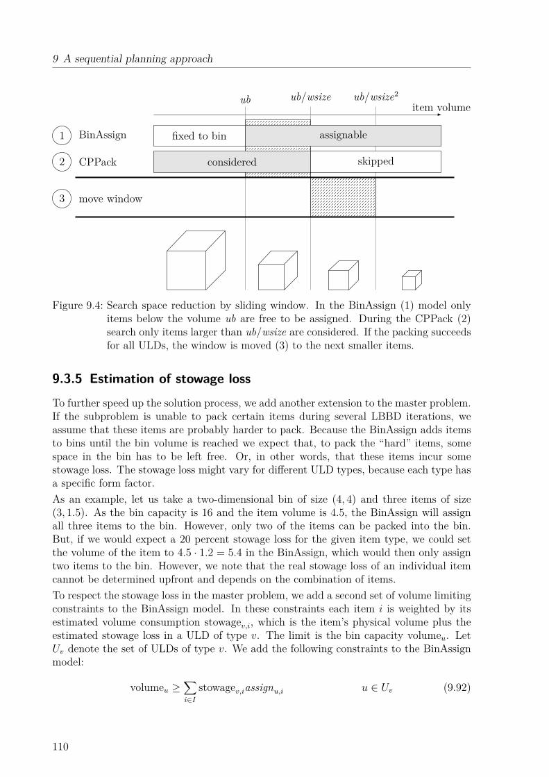
9 A sequential planning approach
ub ub/wsize ub/wsize2
item volume
1 BinAssign fixed to bin assignable
2 CPPack considered skipped
3 move window
Figure 9.4: Search space reduction by sliding window. In the BinAssign (1) model onlyitems below the volume ub are free to be assigned. During the CPPack (2)search only items larger than ub/wsize are considered. If the packing succeedsfor all ULDs, the window is moved (3) to the next smaller items.
9.3.5 Estimation of stowage loss
To further speed up the solution process, we add another extension to the master problem.If the subproblem is unable to pack certain items during several LBBD iterations, weassume that these items are probably harder to pack. Because the BinAssign adds itemsto bins until the bin volume is reached we expect that, to pack the “hard” items, somespace in the bin has to be left free. Or, in other words, that these items incur somestowage loss. The stowage loss might vary for different ULD types, because each type hasa specific form factor.As an example, let us take a two-dimensional bin of size (4, 4) and three items of size(3, 1.5). As the bin capacity is 16 and the item volume is 4.5, the BinAssign will assignall three items to the bin. However, only two of the items can be packed into the bin.But, if we would expect a 20 percent stowage loss for the given item type, we could setthe volume of the item to 4.5 · 1.2 = 5.4 in the BinAssign, which would then only assigntwo items to the bin. However, we note that the real stowage loss of an individual itemcannot be determined upfront and depends on the combination of items.To respect the stowage loss in the master problem, we add a second set of volume limitingconstraints to the BinAssign model. In these constraints each item i is weighted by itsestimated volume consumption stowagev,i, which is the item’s physical volume plus theestimated stowage loss in a ULD of type v. The limit is the bin capacity volumeu. LetUv denote the set of ULDs of type v. We add the following constraints to the BinAssignmodel:
volumeu ≥∑i∈I
stowagev,iassignu,i u ∈ Uv (9.92)
110
9.4 Weight and balance
The question remains how to choose a suitable stowage loss for a given item. For itemsoutside the sliding window we assume no stowage loss. The larger items have already beensuccessfully packed to their assigned bin and smaller items are not considered for packingyet, i.e., we have no information about their packing behavior. We estimate the stowageloss of an item within the sliding window based on the frequency the item appears in thecuts for a specific ULD type. Starting with the original item volume, we multiply theparameter stowagev,i by a constant factor each time the item is part of a generated cut.Hence, the more often an item occurs in an unpackable bin, the higher its stowage lossgets. We reset the stowage loss of each item when the sliding window is moved forward,i.e., when a packable assignment for all currently considered items is found. We analyzesuitable values for the stowage loss factor in our evaluation in Section 10.2.3.
9.3.6 Overall procedure
Finally, we put all the introduced components together and describe our overall procedurefor solving the air cargo palletization. We give a pseudocode description in Algorithm 3.The outer loop (Lines 3 to 21) realizes the sliding window of item sizes. For each entity ofthe sliding window we start with a reset stowage loss and perform an LBBD run (Lines 7to 18) until all items inside the window can be packed. In each LBBD iteration (Lines 10to 17) we solve the BinAssign model and try to pack all selected bins with one CPPacksearch per bin. If the CPPack cannot pack all items, we derive suitable cuts and increasethe items’ stowage loss. If no feasible packing solution is found for a bin, we add the fullset of items assigned to the bin as a cut. The full procedure ends, when the sliding windowreached the smallest items, i.e., when all items have been packed in the subproblem.
9.4 Weight and balance
The final step of our sequential load planning approach is the weight and balance for eachflight. At this stage the ULDs for the different transport segments have been assembledand weighed. Now, for each ULD we need to select a loading position in the aircraft oneach leg of of the flight, such that all technical and regulatory restrictions are fulfilled.We denote this step as UWAB in the following.The remainder of this section is structured as follows. In Section 9.4.1 we introduce somenecessary preprocessing steps to determine suitable model parameters. After that, wepresent the employed MIP model to assign the ULDs to loading positions in Section 9.4.2.
9.4.1 Preprocessing
Before introducing the model itself, we present two preprocessing steps. These stepsderive required model parameters from the solution of the previous air cargo palletizationstep.
111

9 A sequential planning approach
Data: problem instance for one transport segment k, items IkResult: air cargo palletization solution
1 ub ← max({volumei | i ∈ Ik});2 lb ← min({volumei | i ∈ Ik});3 while ub ≥ lb do4 stowage← volume;5 set sliding window of item sizes (Section 9.3.4);6 items ← {i | i ∈ Ik : ub/wsize < volumei ≤ ub};7 do8 solve BinAssign model (Section 9.3.1);9 offloads ← false;
10 for each bin in BinAssign solution do11 solve CPPack model (Section 9.3.2) for items in bin;12 if not all items could be packed then13 generate cuts from bin and add to BinAssign (Section 9.3.3);14 increment stowage loss of items in bin (Section 9.3.5);15 offloads ← true;16 end17 end18 while offloads = true;19 fix items to their currently assigned bin;20 ub ← ub/wstep;21 end
Algorithm 3: Overall procedure to solve the air cargo palletization
112

9.4 Weight and balance
Offload penalties Each item to load has a specific penalty that applies if it is offloaded.As we only deal with ULDs during weight and balance, we sum up the penalties of theitems packed into each ULD to determine the offload penalty of the ULD.
Minimum spacing of ULDs During air cargo palletization we already dealt with in-compatible items that have to be placed into separate ULDs. Some goods also requirenot to be loaded into adjacent ULDs or to have a minimum spacing within the aircraft.Accordingly, we calculate a minimum spacing between two ULDs as the maximum of allpairwise minimum distances of items in the considered ULDs.
9.4.2 Mixed-integer model
We solve the weight and balance by applying the full Weight and Balance Model (WBM)as presented in Section 7.2.5. Table 9.11 recaps the sets and parameters of the model andTable 9.12 presents its decision variables. The model primarily decides about the loadingposition of each ULD on each leg xu,p,l or if the ULD is offloaded xoffu . Auxiliary variableslimiting the aircraft center of gravity (CG) capture the rotational moment of the loadedaircraft ml, the forward (aft) deviation from the optimal CG mlng-
l (mlng+l ), the moment of
inertia mmil , and the total weight of the aircraft wl. Further variables track the necessary
reloading operations after each leg (ql,p, runl,p , ronl,p, rdistl ), the related loading costs opsl, andthe required extra fuel cost due to imbalances fuel+
l .For completeness, we repeat the WBM with minor adjustments for this step:
minimize∑u∈U
aoffu xoffu +∑l∈L
fuel+l +
∑l∈L
opsl +∑l∈L
amil m
mil (9.93)
subject to
xoffu = 1−∑
p∈loadableu
xu,p,l u ∈ U ; l ∈ legsu (9.94)
1 ≥∑u∈U
xu,p,l p ∈ P ; l ∈ L (9.95)
1 ≥∑u∈U
(xu,p,l + xu,p′,l) 〈p, p′〉 ∈ O; l ∈ L (9.96)
MAXl ≥∑u∈U
weightu∑p∈P
xu,p,l l ∈ L (9.97)
limitn ≥∑u∈U
weightu∑p∈P
fn,pxu,p,l n ∈ N ; l ∈ L (9.98)
ml = BAacwOEW + BAfuell FWl
+∑u∈U weightu
∑p∈P BAlng
p xu,p,ll ∈ L (9.99)
wl = wOEW + FWl +∑u∈U
weightu∑p∈P
xu,p,l l ∈ L (9.100)
BAOPTl wl = ml +mlng+
l −mlng-l l ∈ L (9.101)
fuel+l = costfuel−l mlng-
l + costfuel+l mlng+l l ∈ L (9.102)
113

9 A sequential planning approach
Set/Parameter DescriptionL flight legsN set of cumulative weight constraints in the aircraft (n ∈ N)P loading positions in aircraftU ULDs to loadadistl ∈ R cost of working time to move a ULD by one position after leg lamil ∈ R cost of additional fuel depending on the MI on leg laoffu ∈ R penalty when offloading ULD u
aonl ∈ R cost of one ULD loading operation after leg launl ∈ R cost of one ULD unloading operation after leg lBp ⊆ P blocking positions when (un)loading a ULD at position pBAac ∈ R longitudinal balance arm of the empty aircraft (OEW)BAfuel
l ∈ R≥0 longitudinal balance arm of the aircraft’s fuel tanksBAlat
p ∈ R lateral balance arm of loading position pBAlng
p ∈ R longitudinal balance arm of loading position pBAMAX
l ∈ R≥0 maximum allowed lateral CG imbalance on leg lBAOPT
l ∈ R optimal longitudinal CG on leg lcostfuel−l ∈ R≥0 cost of extra fuel for forward CG deviations on leg lcostfuel+l ∈ R≥0 cost of extra fuel for aft CG deviations on leg ldistp ∈ R≥0 distance between position and doordistp,p′ ∈ R≥0 distance between loading positionsfn,p ∈ R factor of loading position p for constraint nFWl ∈ R≥0 fuel weight loaded on leg llegsu ⊆ L legs the ULD will be on boardlimitn ∈ R cumulative weight limit of constraint nloadableu ⊆ P loading positions available for ULD u
MAXl ∈ R maximum loadable ULD weight on leg lMAXCGl ∈ R aft limit of the longitudinal CG on leg lminu,u′ ∈ R≥0 minimum distance of separation constraintMINCGl ∈ R forward limit of longitudinal CG on leg lO ⊆ P × P set of overlapping loading positions (〈p, p′〉 ∈ O)Rp ⊆ P set of loading positions that position p depends onS ⊆ U × U set of ULDs to separate (〈u, u′〉 ∈ S)wOEW ∈ R≥0 operating empty weight (OEW) of the aircraftweightu ∈ R≥0 total weight of ULD u
Table 9.11: Parameters of the weight and balance model
114

9.4 Weight and balance
Variable Descriptionfuel+
l ∈ R≥0 cost of required extra fuel on leg lml ∈ R≥0 longitudinal rotational moment of loaded aircraft on leg lmlat-l ∈ R≥0 left lateral imbalance from aircraft center on leg l
mlat+l ∈ R≥0 right lateral imbalance from aircraft center on leg l
mlng-l ∈ R≥0 forward deviation of rotational moment from optimal CG on leg l
mlng+l ∈ R≥0 aft deviation of rotational moment from optimal CG on leg l
mmil ∈ R≥0 moment of inertia of the loaded ULDs on leg l
opsl ∈ R≥0 extra handling cost after leg lql,p ∈ {0, 1} 1 if loading position p needs to be cleared after leg lrunl,p ∈ {0, 1} 1 if a ULD is unloaded from position p after leg lronl,p ∈ {0, 1} 1 if a ULD is loaded on position p after leg lrdistl ∈ R≥0 total ULD move distance after leg lwl ∈ R≥0 total weight of loaded aircraft of leg lxu,p,l ∈ {0, 1} 1 if ULD u is loaded at position p on leg lxoffu ∈ {0, 1} 1 if ULD u is not transported
Table 9.12: Decision variables of the weight and balance model
ml ≤ MAXCGlwl l ∈ L (9.103)ml ≥ MINCGlwl l ∈ L (9.104)
mlat+l =
∑p∈P
weightu∑u∈U
BAlatp xu,p,l +mlat-
l l ∈ L (9.105)
BAMAXl wl ≥ mlat+
l +mlat-l l ∈ L (9.106)
mmil =
∑u∈U
weightu∑p∈P
(BAOPTl − BAlng
p )2xu,p,l l ∈ L (9.107)∑u∈U
xu,p,l ≤∑p′∈Rp
∑u∈U
xu,p′,l p ∈ P ; l ∈ L (9.108)
1 ≥∑p′∈P :
distp,p′<minu,u′
xu,p,l + xu′,p′,l 〈u, u′〉 ∈ S; p ∈ P ; l ∈ L (9.109)
ql,p ≥ xu,p,l − xu,p,l+1 u ∈ U ; p ∈ P ; l ∈ L (9.110)ql,p ≥ xu,p,l+1 − xu,p,l u ∈ U ; p ∈ P ; l ∈ L (9.111)ql,p ≤ ql,p′ p ∈ P ; p′ ∈ Bp; l ∈ L (9.112)ql,p ≤ ql,p′ p ∈ P ; p′ ∈ Bp; l ∈ L (9.113)runl,p ≥ ql,p +
∑u∈U
xu,p,l − 1 p ∈ P ; l ∈ L (9.114)
ronl,p ≥ ql,p +∑u∈U
xu,p,l+1 − 1 p ∈ P ; l ∈ L (9.115)
115

9 A sequential planning approach
rdistl =∑p∈P
distp(runl,p + ronl,p) l ∈ L (9.116)
opsl = aunl∑p∈P
runl,p + aonl∑p∈P
ronl,p + adistl rdistl l ∈ L (9.117)
fuel+l , opsl, rdistl ∈ R≥0 l ∈ L (9.118)
ml,mlat-l ,mlat+
l ,mlng-l ,mlng+
l ,mmil , wl ∈ R≥0 l ∈ L (9.119)
ql,p, runl,p , r
onl,p ∈ {0, 1} l ∈ L; p ∈ P (9.120)
xu,p,l ∈ {0, 1} u ∈ U ; p ∈ P ; l ∈ L (9.121)xoffu ∈ {0, 1} u ∈ U (9.122)
The objective, given in Equation (9.93), is to minimize the sum of additional costs ofthe flight. These costs may arise from offloaded ULDs, the extra fuel consumed due toimbalance, extra handling operations to reload ULDs inside the aircraft between legs, anda penalty proportional to the moment of inertia of the aircraft. In the following we brieflydescribe the restrictions. For an in depth explanation and motivation of the constraintswe refer to Section 7.2.3.The unique assignment of each ULD is modeled in Equations (9.94) and (9.95). Themutual exclusion of overlapping loading positions is enforced by Equation (9.96). Equa-tions (9.97) and (9.98) track the total and cumulative weights of loaded ULDs. Equa-tions (9.99) to (9.104) model the extra fuel required due to the position of the longitu-dinal CG of the aircraft. The lateral imbalance of the aircraft is restricted with Equa-tions (9.105) and (9.106). Equation (9.107) models the moment of inertia of the aircraft.Interdependent loading positions are enforced by Equation (9.108). Minimum requireddistances of ULDs are handled within Equation (9.109). Finally, Equations (9.110) to(9.117) model the required handling operations to load and unload the ULDs between therespective legs of the flight.
9.5 SummaryIn this chapter, we introduced a first solution approach for the Air Cargo Load PlanningProblem (ACLPP) denoted as SeqACLPP. It consists of a sequential four-step planningpipeline that follows the current manual processes in operational practice.For the first step, dealing with the aircraft configuration, denoted as VWAC, we presenteda MIP model that selects the number of ULDs of each type to build for each transportsegment of a flight based on aggregated booking data. The selected ULDs together withthe arrival times of the cargo and departure time of the flights build the input for thenext step.To solve the second step, dealing with the build-up scheduling, denoted as RHBS, weintroduced a rolling horizon planning approach that determines the ULD build-up starttimes for all flights departing during the planning horizon. In each round we apply a MIPmodel solving one shift while also taking the demand of the next n shifts into account.For the third step, dealing with the air cargo palletization, denoted as BDAP, we realizeda Logic-based Benders Decomposition approach. The LBBD master problem is a MIP
116

9.5 Summary
containing a vector container loading problem that assigns items to ULDs. In the masterproblem all non-geometric aspects like weights, time, sorting and compatibilities are han-dled. The LBBD subproblem, which is solved for each ULD individually, is implementedas a constraint program and solves the three-dimensional knapsack problem. In it wedeal with all the geometric aspects as well as stacking and stability issues. If some itemscannot be packed into the ULD in a subproblem, we heuristically derive cuts, add themto the master problem, and solve it again. To make the solution process come to an endwithin a reasonable amount of time we introduced two extensions. The first reduces thesearch space by considering only a part of the items during each iteration. The secondincreases the virtual volume of items that repeatedly cause problems during the packing.For the forth step, dealing with the weight and balance, denoted as UWAB, we presenteda MIP model that assigns the weighed ULDs to loading positions of the aircraft. Themodel can handle flights with an arbitrary number of legs at once and minimizes the totalcost caused by additional fuel required due to aircraft imbalances and necessary reloadingoperations at stop-over airports to access ULDs.
117

10 Evaluation
In this chapter, we describe our experimental setup and the achieved results. We im-plemented the SeqACLPP approach introduced in Chapter 9 and evaluated it on thebenchmark instances described in Chapter 8. To evaluate its applicability for operationalpractice, we compare the achieved solution quality to real-world solutions. Furthermore,we survey the achieved solution quality for the introduced scenarios and discuss the re-quired runtimes. Before we ran our experiments, we performed an extensive parametertuning to choose suitable configuration settings for the SeqACLPP approach.This chapter is organized as follows: First, we describe our implementation and testingenvironment in Section 10.1. Afterwards, we introduce our preliminary tests to determinesuitable parameter settings values for the SeqACLPP approach in Section 10.2. Finally,we describe the results achieved with the SeqACLPP approach in Section 10.3.
10.1 Implementation and testing environment
We implemented all presented models in C++ using the Visual Studio 2012 compilerwith standard Release mode settings. All executables were built in 32-bit mode. As MIPsolver we employed Gurobi in version 7.0.1. Gurobi was set to use only a single thread,to stop at a 1 percent MIP gap, and to spend 95 percent of the time with heuristics. Allother parameters remained at their default values. For the constraint program introducedin Section 9.3.2 we used Gecode, an open-source constraint programming framework, inversion 4.4.0 with its standard branch and bound search.We performed our experiments on two types of machines. The smaller machines had oneIntel Core i5-760 processor with 4 cores clocked at 2.8 GHz and equipped with 8 MBcache. Each machine had 8 GB main memory and was running on a 64-bit Windows 7Professional. The bigger machine had two Intel Xeon E5-2650 v2 processors each with8 cores clocked at 2.6 GHz and equipped with 20 MB cache. The machine had 128 GBmain memory and was running on a 64-bit Windows Server 2012. In total we employedsix machines of the smaller and one of the bigger type. All machines were simultane-ously executing as many solution processes as they had cores, i.e., all experiments wereperformed under full load. Accordingly, the presented runtimes can be seen as a con-servative benchmark originating from adverse conditions. The differences of the averageruntimes seen across all the used machines were less than 15 percent. Therefore, we omita breakdown of the runtimes by machines in the following.

10 Evaluation
Option ValueAircraft configuration (VWAC)
estimated achievable volume utilization in percent 66Build-up scheduling (RHBS)
planning horizon in shifts 3MIP time limit in seconds 900
Palletization (BDAP)size of the sliding window of item sizes 1.1stowage loss increment factor 1.02BinAssign initial time limit in seconds 300BinAssign warm start time limit in seconds 60CPPack time limit in seconds 1
Weight and balance (UWAB)MIP time limit in seconds 300
Table 10.1: Parameters of the SeqACLPP and their values chosen for evaluation
10.2 Preliminary parameter tuning
As shown in Table 10.1 the SeqACLPP approach is configurable in many ways. Beforerunning our main evaluation, we performed preliminary experiments to identify and selectsuitable values for those parameters. In the following we describe those experiments andintroduce the chosen parameter values for the aircraft configuration, build-up scheduling,palletization, and weight and balance steps.
10.2.1 Aircraft configuration
The volume-and-weight-based aircraft configuration (VWAC) step, presented in Sec-tion 9.1, operates on the estimated achievable volume utilization of the ULDs. In thissection, we discuss how to find a suitable utilization parameter value. Our hypothesis isthat the net load factor (NLF) of previous flights provides a good estimate.In a first test, we verified this hypothesis by performing tests for different parametersettings on the real world flights of our dataset A base scenario (A-base). In the solutionsseen in practice for the A-base flights, the NLF was around 55 percent. Therefore, wevaried the utilization parameter around this value in our experiments. The resultingnumbers of selected ULDs are shown in Figure 10.1. As one would expect, lower achievableutilizations lead to more selected ULDs. Furthermore, the aircraft configurations selectedby the model with 55 percent utilization come closest to the real-world results. Therefore,we argue that the VWAC produces realistic configurations if it is parameterized with arealistic NLF.Looking into the details at 55 percent utilization we see that the VWAC selects about24 percent more of the large PGE ULDs (141 instead of 114) and about 34 percent lessof the small AKE ULDs (52 instead of 79) than were built in reality. We attribute this to
120
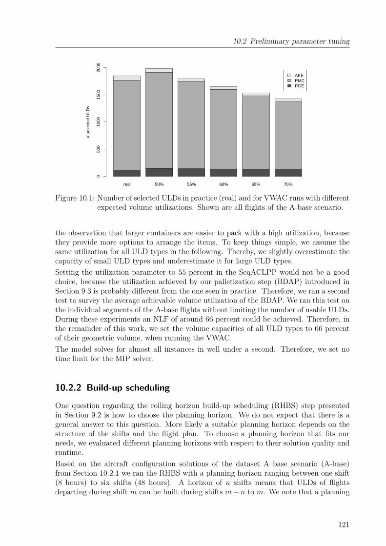
10.2 Preliminary parameter tuning
real 50% 55% 60% 65% 70%
AKEPMCPGE
avg. expected ULD utilization
# se
lect
ed U
LDs
050
010
0015
0020
00
Figure 10.1: Number of selected ULDs in practice (real) and for VWAC runs with differentexpected volume utilizations. Shown are all flights of the A-base scenario.
the observation that larger containers are easier to pack with a high utilization, becausethey provide more options to arrange the items. To keep things simple, we assume thesame utilization for all ULD types in the following. Thereby, we slightly overestimate thecapacity of small ULD types and underestimate it for large ULD types.Setting the utilization parameter to 55 percent in the SeqACLPP would not be a goodchoice, because the utilization achieved by our palletization step (BDAP) introduced inSection 9.3 is probably different from the one seen in practice. Therefore, we ran a secondtest to survey the average achievable volume utilization of the BDAP. We ran this test onthe individual segments of the A-base flights without limiting the number of usable ULDs.During these experiments an NLF of around 66 percent could be achieved. Therefore, inthe remainder of this work, we set the volume capacities of all ULD types to 66 percentof their geometric volume, when running the VWAC.The model solves for almost all instances in well under a second. Therefore, we set notime limit for the MIP solver.
10.2.2 Build-up scheduling
One question regarding the rolling horizon build-up scheduling (RHBS) step presentedin Section 9.2 is how to choose the planning horizon. We do not expect that there is ageneral answer to this question. More likely a suitable planning horizon depends on thestructure of the shifts and the flight plan. To choose a planning horizon that fits ourneeds, we evaluated different planning horizons with respect to their solution quality andruntime.Based on the aircraft configuration solutions of the dataset A base scenario (A-base)from Section 10.2.1 we ran the RHBS with a planning horizon ranging between one shift(8 hours) to six shifts (48 hours). A horizon of n shifts means that ULDs of flightsdeparting during shift m can be built during shifts m− n to m. We note that a planning
121

10 Evaluation
1 (8H) 2 (16H) 3 (24H) 4 (32H) 5 (40H) 6 (48H)
nightlateearly
cost
s re
lativ
e to
bes
t sol
utio
n
124.8%
102.4% 100.5% 100% 100.5% 100.5%
Figure 10.2: Costs of crews required for different planning horizons
1 (8H) 2 (16H) 3 (24H) 4 (32H) 5 (40H) 6 (48H)
planning horizon
runt
ime
per
itera
tion
[sec
]
050
100
150
200
0 2.5
22.5
46.3
68
182
Figure 10.3: Runtimes per shift for different planning horizons
horizon of 0 is not useful. In this case it would not be possible to build ULDs of flightsdeparting early in a shift during the previous shift, which is necessary in practice.As it is common practice we use three shifts per day: an early (06:00 to 14:00), late (14:00to 22:00), and night (22:00 to 06:00) shift. For our experiments, we expect the cost of anight shift to be 20 percent above the cost of the other shifts. An overview of the costsof the selected crews per shift for different planning horizons is given in Figure 10.2. Allnumbers are given relative to the best found solution, which had a planning horizon offour shifts (32 hours).As expected, shorter planning horizons give worse results, but from three shifts on thequality is nearly constant. Interestingly, the number of late shifts for a planning horizonof one shift is almost twice as high as for all others. We attribute this to two effects. First,instead of the more expensive night shifts the model selects more late shifts. Accordingly,a planning horizon of 1 shift shows the lowest number of night shifts. The second effect isthat, with a planning horizon of one shift, flights departing during the late shifts cannotbe built during the night shift before, although a significant amount of their cargo has
122

10.2 Preliminary parameter tuning
already arrived. But, during the night there are only a few departing flights in the scheduleof the A-base scenario and thus the selected crews often cannot be fully utilized.Besides the solution quality, we are interested in the runtime of the RHBS to decideabout a suitable planning horizon. Remember from Figure 9.1, that we solve the Build-up Scheduling Model (BSM) in a rolling horizon approach, i.e., we execute it successivelyfor each shift with a lookahead of a planning horizon of n shifts. Figure 10.3 shows theaverage runtime required for one BSM run for different planning horizons. We stoppedthe search after 900 seconds or when the MIP gap became smaller than 1 percent. Asone would expect the runtime grows exponentially for larger planning horizons. We notethat for planning the shifts of one week we must run 21 iterations, i.e., planning with a48 hours horizon takes more than 1 hour.Given the above insights into solution quality and runtime we select a planning horizonof 3 shifts, or 24 hours respectively, for the remainder of this work.
10.2.3 Palletization
The Logic-based Benders Decomposition (LBBD) solving the palletization (BDAP), whichwe presented in Section 9.3.3, has five parameters for which we need to identify suitablevalues. First, there is the size of the sliding window of item volume. During each iteration,only items within the window are considered for assignment and packing. Larger itemshave a fixed assignment while smaller items are not considered during packing.The second parameter is the stowage loss factor. After each failed ULD packing, i.e.,where some items could not be placed into the assigned ULD, we multiply the virtualvolume of all items assigned to this ULD by an expected stowage loss factor. Accordingly,in upcoming BinAssign iterations, less of these items will be assigned to the ULD andthus it should become easier to find a feasible packing.The other parameters limit the runtime: a cold start and warm start time limit for theBinAssign MIP model and a time limit for the CPPack search.To find suitable parameter settings with tolerable effort we randomly selected 30 flightsfrom our datasets, 5 of each scenario, and solved those flights for different parametervalues. We repeated the experiments three times and show the average values in thefollowing. In the remainder of this section we present the achieved results and justify ourchoice of parameters.
Sliding window size
First, we analyze the effects of different sizes of the sliding window of item volume. Asintroduced in Algorithm 3, the window size determines the number of successive runs ofthe LBBD to process all items, starting with the biggest items in the first run and thenmoving to smaller items. The window during an LBBD run is defined as (ub/wsize, ub]for a window size wsize and upper bound ub. As stated above, only items with a volumewithin the window are considered for the bin assignment and packing. Thus, the windowsize determines the number of items handled during each iteration. A larger window sizeleads to larger subproblems in each iteration, but also fewer shifts of the window are
123

10 Evaluation
1.05 1.1 1.25 1.5 1.75 2 2.5
avg.
pen
alty
per
inst
ance
020
0040
0060
0080
0010
000
1200
09692
9119
990510356
9563 972110391
Figure 10.4: Penalties for different window sizes
necessary until all items have been covered. On our sample instances we evaluated theSeqACLPP approach for varying values of wsize ranging between 1.05 and 2.5. In thefollowing, we discuss the impact of the different values on solution quality and requiredeffort.The first thing we note is that there is no clear relationship between the window size andsolution quality. Figure 10.4 shows the average offload penalty of our sample instancesfor the different sizes. All values are within a range of 12 percent. One explanation ofthis effect might be the large number of items in the instances. Even if only a part of theitems is considered at each sliding window position, the remaining solution space seemsto contain many alternative solutions of similar quality.As one would expect, the required number of total LBBD iterations, i.e., the sum of iter-ations of all LBBD runs, of Algorithm 3 decreases with a larger window size. Figure 10.5shows the average total LBBD iterations it takes to solve the sample instances for dif-ferent window sizes. However, this decrease is not linear. Larger window sizes requireless LBBD runs with different volume windows, but lead to more infeasible packings andthus more LBBD iterations in each run for adding cuts before a feasible packing is found.Figure 10.6 presents the average number of iterations the LBBD takes for a run beforethe packings can be solved successfully.Furthermore, there is a tradeoff between window size and solution runtime, with a windowsize of 1.25 showing the shortest runtimes. Figure 10.7 shows the respective averageruntimes. At small window sizes, the high number of total LBBD iterations lead to highruntimes. Larger window sizes also increase runtimes, because more items have to beconsidered in the BinAssign model and thus each iteration takes longer. Given the resultsabove, we choose a value of 1.1 as the size of the sliding window in the remainder of thiswork. This setting showed the lowest penalty and the second best runtimes.
Stowage loss factor
Next, we analyze the impact of different settings for the stowage loss factor on solutionquality and effort. As introduced in Section 9.3.1, in the LBBD master problem, the
124
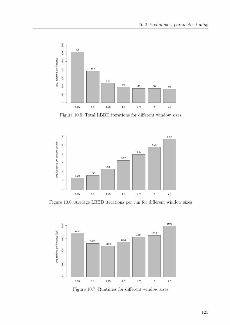
10.2 Preliminary parameter tuning
1.05 1.1 1.25 1.5 1.75 2 2.5
avg.
iter
atio
ns p
er in
stan
ce
050
100
150
200
250
300
350
309
193
118
9586 86 83
Figure 10.5: Total LBBD iterations for different window sizes
1.05 1.1 1.25 1.5 1.75 2 2.5
avg.
iter
atio
ns p
er w
indo
w p
ositi
on
01
23
45
6
1.291.58
2.3
3.27
3.97
4.76
5.67
Figure 10.6: Average LBBD iterations per run for different window sizes
1.05 1.1 1.25 1.5 1.75 2 2.5
avg.
run
time
per
inst
ance
[sec
]
050
010
0015
0020
00
1680
13031198
1351
15541616
1976
Figure 10.7: Runtimes for different window sizes
125

10 Evaluation
1 1.01 1.02 1.05 1.1 1.2 1.5
avg.
pen
alty
per
inst
ance
020
0040
0060
0080
0010
000
1200
09823 10060
91199756 9510 9594 9566
Figure 10.8: Penalties for different stowage loss factors
BinAssign model, we solve a vector container loading problem with respect to item volumeand weight. If the assignment result cannot be packed by the CPPack subproblem, weassume that the assigned items incur some stowage loss. To overcome this in the nextLBBD iteration, we increase the item volume considered in the master problem by a factorstow. The more often an item occurs in unpackable bins, the higher its stowage loss gets.Accordingly, larger factors should result in less required iterations before a feasible three-dimensional packing can be found. On our sample instances we evaluated the SeqACLPPapproach for varying values of stow between 1.0 and 1.5, representing a volume incrementbetween 0 and 50 percent for each failed packing attempt.As the first result we note, similar to the window size, that there is no clear relationshipbetween the stowage loss factor and solution quality. Figure 10.8 shows the average offloadpenalty of our sample instances for different factors. As for the window size, we assumethat this effect stems from the large number of items in the instances. Even if an increasedstowage loss cuts of promising solutions, the remaining solution space seems to containmany alternative solutions of similar quality.The required number of total LBBD iterations, i.e., the sum of iterations of all LBBDruns, of Algorithm 3 decreases slightly for higher stowage loss factors. Figure 10.9 showsthe average number of total iterations it takes to solve the sample instances. For smallvalues between 1.01 and 1.05 the number of required iterations does not change at all.The same picture shows for the average number of iterations the LBBD takes for a run,i.e., before the packings can be solved successfully, which is shown in Figure 10.10. Again,higher values lead to less iterations, because the stowage loss rises faster.Regarding the total solution runtime, we see a clear drop from more than 1,600 seconds toaround 1,300 seconds when the stowage loss factor is used. For larger factors the runtimedecreases slowly in the same way as the number of required iterations. Figure 10.11 showsthe respective average runtimes. According to the found results, we choose a value of 1.02for the stowage loss factor in the remainder of this work.
126

10.2 Preliminary parameter tuning
1 1.01 1.02 1.05 1.1 1.2 1.5
avg.
iter
atio
ns p
er in
stan
ce
050
100
150
200 201
193 193 193184
177167
Figure 10.9: Total LBBD iterations for different stowage loss factors
1 1.01 1.02 1.05 1.1 1.2 1.5
avg.
iter
atio
ns p
er w
indo
w p
ositi
on
0.0
0.5
1.0
1.5
1.671.58 1.58 1.6
1.511.44
1.35
Figure 10.10: Average LBBD iterations per run for different stowage loss factors
1 1.01 1.02 1.05 1.1 1.2 1.5
avg.
run
time
per
inst
ance
[sec
]
050
010
0015
00
1656
1288 1303 13441249 1254
1132
Figure 10.11: Runtimes for different stowage loss factors
127
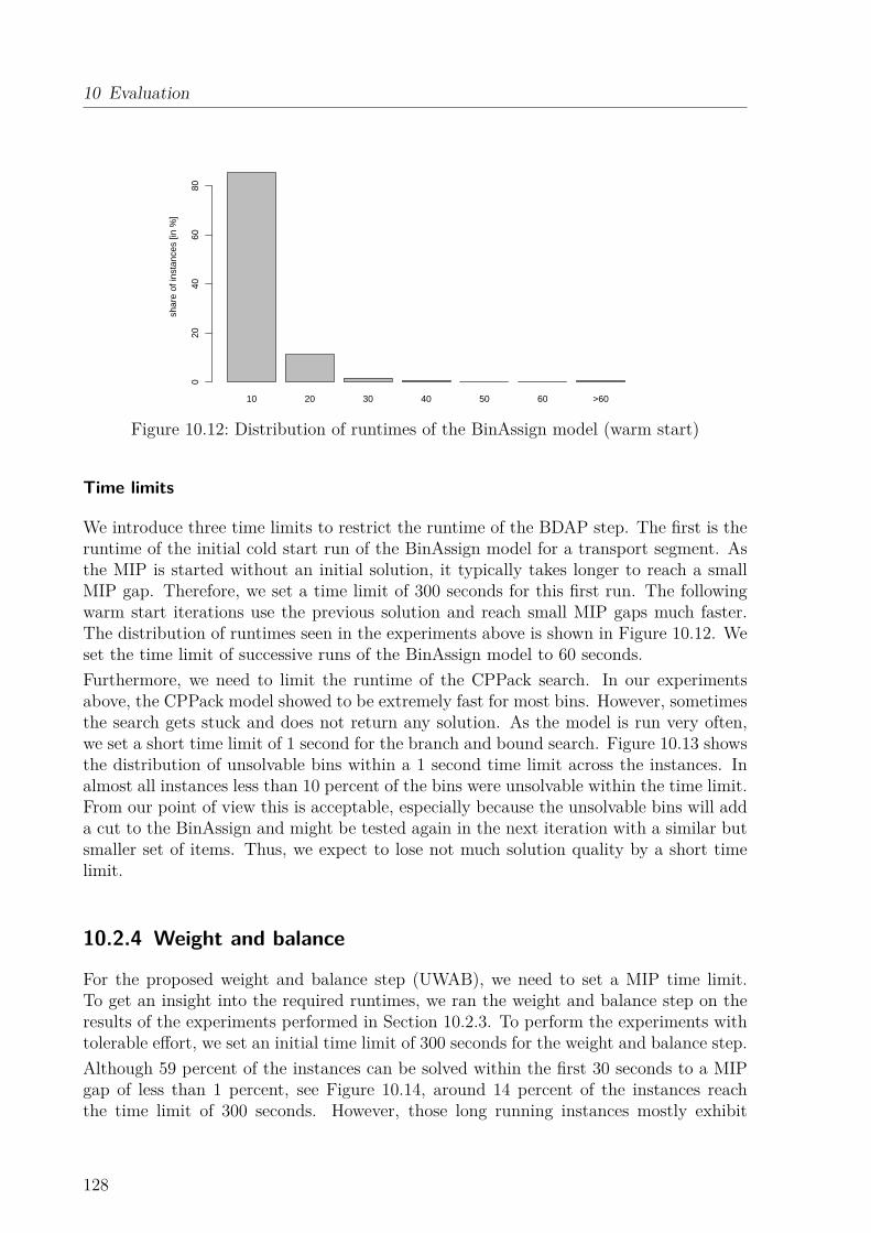
10 Evaluation
10 20 30 40 50 60 >60
shar
e of
inst
ance
s [in
%]
020
4060
80
Figure 10.12: Distribution of runtimes of the BinAssign model (warm start)
Time limits
We introduce three time limits to restrict the runtime of the BDAP step. The first is theruntime of the initial cold start run of the BinAssign model for a transport segment. Asthe MIP is started without an initial solution, it typically takes longer to reach a smallMIP gap. Therefore, we set a time limit of 300 seconds for this first run. The followingwarm start iterations use the previous solution and reach small MIP gaps much faster.The distribution of runtimes seen in the experiments above is shown in Figure 10.12. Weset the time limit of successive runs of the BinAssign model to 60 seconds.Furthermore, we need to limit the runtime of the CPPack search. In our experimentsabove, the CPPack model showed to be extremely fast for most bins. However, sometimesthe search gets stuck and does not return any solution. As the model is run very often,we set a short time limit of 1 second for the branch and bound search. Figure 10.13 showsthe distribution of unsolvable bins within a 1 second time limit across the instances. Inalmost all instances less than 10 percent of the bins were unsolvable within the time limit.From our point of view this is acceptable, especially because the unsolvable bins will adda cut to the BinAssign and might be tested again in the next iteration with a similar butsmaller set of items. Thus, we expect to lose not much solution quality by a short timelimit.
10.2.4 Weight and balance
For the proposed weight and balance step (UWAB), we need to set a MIP time limit.To get an insight into the required runtimes, we ran the weight and balance step on theresults of the experiments performed in Section 10.2.3. To perform the experiments withtolerable effort, we set an initial time limit of 300 seconds for the weight and balance step.Although 59 percent of the instances can be solved within the first 30 seconds to a MIPgap of less than 1 percent, see Figure 10.14, around 14 percent of the instances reachthe time limit of 300 seconds. However, those long running instances mostly exhibit
128

10.3 Results of the sequential approach
1 2 3 4 5 6 7 8 9 10 >10
shar
e of
inst
ance
s [in
%]
05
1015
2025
Figure 10.13: Distribution of the share of unsolvable bins per instance for CPPack with atime limit of 1 second (in %)). To be read as: in 24 percent of all instancesbetween 1 and 2 percent of the bins could not be solved within 1 second.
30 60 90 120 150 180 210 240 270 300 >300
shar
e of
inst
ance
s [in
%]
010
2030
4050
60
Figure 10.14: Distribution of runtimes of the weight and balance step (in sec)
small MIP gaps, see Figure 10.15. Around 70 percent of them have a gap smaller than10 percent. Therefore, in our evaluation we keep the initial time limit of 300 seconds.
10.3 Results of the sequential approach
We evaluated our approach on the two datasets introduced in Section 8.3. First, we relateour results to actual load plans seen in practice to check the plausibility of our solutions.Afterwards, we discuss the results achieved for the different scenarios.
129

10 Evaluation
10 20 30 40 50 60 70 80 90 100
shar
e of
inst
ance
s [in
%]
010
2030
4050
6070
Figure 10.15: Distribution of the remaining MIP gap of flights reaching a time limit of300 seconds for the weight and balance step (in %)
Real-world SeqACLPP ∆solutions approach
WLF 0.495 0.493 -0.4%GLF 0.327 0.322 -1.5%NLF 0.546 0.662 +21.2%UNITS 23.000 15.685 -31.8%SPLIT 0.283 0.201 -29.0%DISP 3.100 2.585 -16.6%MIX 0.173 0.116 -32.9%CREWS n/a 211 n/a
Table 10.2: Performance of the SeqACLPP approach compared to results seen in practice
Comparison to practice
We compare our results of the real world dataset base scenario (A-base) with the actualsolutions created by load planners and palletization workers in practice. Table 10.2 givesan overview of the respective performance indicators.With regard to the aircraft utilization indicators, the weight load factor (WLF) andvolume gross load factor (GLF) cannot be further improved, because the given flightinstances contained only the transported items of the real flights. Some items, representingaround 0.4 percent of the weight and 1.5 percent of the volume, that were loaded inpractice were offloaded by our approach. For these cases we identify three reasons. First,the workers in practice are more flexible than the SeqACLPP approach. For example,they can postpone a ULD to wait for a late item or add dunnage material to provide aneven surface for a large and light item. Second, there might be errors in the booking datathat made the real packing easier. Maybe, some items in reality were smaller than in thebooking data or one large booked item turned out to be a set of smaller items. Third,
130
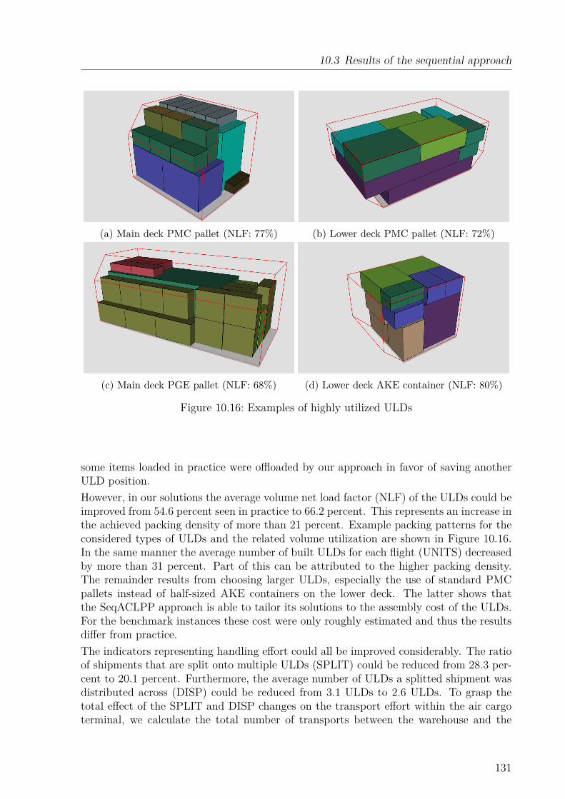
10.3 Results of the sequential approach
(a) Main deck PMC pallet (NLF: 77%) (b) Lower deck PMC pallet (NLF: 72%)
(c) Main deck PGE pallet (NLF: 68%) (d) Lower deck AKE container (NLF: 80%)
Figure 10.16: Examples of highly utilized ULDs
some items loaded in practice were offloaded by our approach in favor of saving anotherULD position.However, in our solutions the average volume net load factor (NLF) of the ULDs could beimproved from 54.6 percent seen in practice to 66.2 percent. This represents an increase inthe achieved packing density of more than 21 percent. Example packing patterns for theconsidered types of ULDs and the related volume utilization are shown in Figure 10.16.In the same manner the average number of built ULDs for each flight (UNITS) decreasedby more than 31 percent. Part of this can be attributed to the higher packing density.The remainder results from choosing larger ULDs, especially the use of standard PMCpallets instead of half-sized AKE containers on the lower deck. The latter shows thatthe SeqACLPP approach is able to tailor its solutions to the assembly cost of the ULDs.For the benchmark instances these cost were only roughly estimated and thus the resultsdiffer from practice.The indicators representing handling effort could all be improved considerably. The ratioof shipments that are split onto multiple ULDs (SPLIT) could be reduced from 28.3 per-cent to 20.1 percent. Furthermore, the average number of ULDs a splitted shipment wasdistributed across (DISP) could be reduced from 3.1 ULDs to 2.6 ULDs. To grasp thetotal effect of the SPLIT and DISP changes on the transport effort within the air cargoterminal, we calculate the total number of transports between the warehouse and the
131

10 Evaluation
A-base A-high A-fast B-base B-high B-fastWLF 0.493 0.969 0.492 0.501 0.966 0.506GLF 0.322 0.680 0.322 0.346 0.672 0.346NLF 0.662 0.709 0.668 0.664 0.695 0.661UNITS 15.685 31.854 15.607 16.585 32.549 16.793SPLIT 0.201 0.259 0.210 0.206 0.256 0.198DISP 2.585 2.966 2.554 2.552 2.849 2.577MIX 0.116 0.119 0.119 0.117 0.141 0.124CREWS 211 410 227 215 391 276
Table 10.3: Performance of the SeqACLPP approach across all scenarios
workstations, which can be defined as:
SPLIT ·DISP + (1− SPLIT) · 1 (10.1)
It represents the average number of warehouse to ULD workstation transports for splittedshipments and a single transport for non-splitted shipments. Compared to the currentpractice, our results realize a reduction of transports of more than 17 percent.The ratio of ULDs that contain both standard and premium shipments (MIX) couldbe reduced from 17.3 percent to 11.6 percent. Together with the reduction of handledUNITS, this results in around 2 ULDs less per flight that would need preferred expresshandling and thus incur higher cost.With respect to the required crews, we cannot make any statement. In practice, thebuild-up crews are also used for other tasks, for example, in the break-down of incomingULDs, and thus no specific number of build-up crews was available to us.Besides the numbers, we also discussed individual load plans with the respective expertsof our industrial partner who found the results to be reasonable. In general, we can saythat the SeqACLPP approach works and provides solutions showing better performancevalues than the current practice.
Scenario evaluation
As the second step of our evaluation, we analyze the results of the SeqACLPP approachfor the respective scenarios defined in Section 8.3.3. Table 10.3 shows the achieved per-formance values.In the base and fast scenarios of both datasets the achieved utilization with respect tothe aircraft weight (WLF) and volume (GLF and NLF) capacity is pretty stable. Almostall items are loaded and an NLF between 66.1 percent and 66.8 percent is achieved. Inthe high-load scenarios much more cargo has to be offloaded, because all the flights areoverbooked. Nevertheless, our approach utilizes more than 96 percent of the aircraftweight capacity (WLF) and fills on average 69.5 percent and 70.9 percent of the physicalvolume of the ULDs (NLF), which is slightly better than in the base and fast scenarios.According to practitioners, utilizing 70 percent of the volume of a single ULD is alreadya very good result.
132

10.3 Results of the sequential approach
A-base A-high A-fast B-base B-high B-fastPEN 2807.000 20407.000 2774.000 3006.000 40035.000 2200.000UNITS 3680.899 7238.202 3633.708 4070.732 7531.707 3950.000FUEL 20.438 417.213 38.169 56.988 465.890 44.500OPS 83.258 166.506 68.652 91.939 247.293 99.854TOTAL 6591.595 27310.921 6513.529 7225.659 48279.890 6294.354
Table 10.4: Cost of the SeqACLPP approach across all scenarios
The aircraft type used in our experiments had a standard configuration of 3 PGE, 20 maindeck PMC, and 10 lower deck PMC ULDs, totaling 33 units. Accordingly, almost all load-ing positions are used in the high-load flights. Therefore, we conclude that the SeqACLPPapproach is able to find good solutions, which are also well-balanced with respect to theweight and volume capacities of the aircraft.The indicators representing handling effort, namely SPLIT, DISP, and MIX, are simi-lar across all scenarios, indicating that these objectives can also be robustly improvedcompared to the current manual practice.The number of crews employed in the scenarios correlates with the built ULDs. Crewproductivity for all scenarios ranges between 5.0 and 6.9 ULDs per crew and shift. Thefast scenarios show the lowest productivity with 6.1 and 5.0 ULDs per crew and shift.The reason here clearly is the unleveled workload stemming from the short transfer timesof the cargo. During rush hours a high number of crews is needed, but before and afterthe crews are idling.Next, we look at the total costs achieved by the SeqACLPP approach. Table 10.4 showsthe respective average values for each scenario. A significant part of the costs stems fromthe penalties of offloaded items (PEN). While this is reasonable for the overbooked high-load scenarios, this result is not satisfactory for the base and fast scenarios. Analyzingthe results in detail, we identified two primary reasons for offloaded items.First, during aircraft configuration the capacity to accommodate large items is overes-timated. We only consider the item volume and weight here, neglecting the real itemdimensions. Thereby, the model is too optimistic when selecting ULDs for large items.Later, during palletization these items cannot be combined on ULDs and some of themmust be offloaded. In the fast scenarios, we see less offloads, because the ULDs aregenerally built later and therefore more combinations of items are possible.The second reason causing significant offloads in our solutions are too heavy ULDs createdby the palletization step for which no loading position in the aircraft can be found duringthe weight and balance step. While the individual weight limit of a ULD type is quitehigh, for example, a main deck PMC pallet can weight up to 6,800 kg, the possible loadingpositions for heavy ULDs are very limited. Only four of the 26 positions on the maindeck of our sample MD11F aircraft can handle this weight. Furthermore, the cumulativeload limits of adjacent positions reduce the solution space significantly. For example,only two of the four positions mentioned above can be used simultaneously for suchheavy ULDs without violating the maximum running load along the aircraft fuselage. Onsome positions the combined weight limit of two adjacent ULDs is less than 125 percent
133
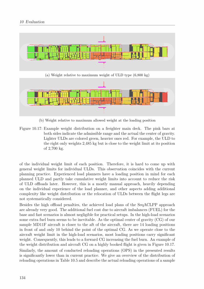
10 Evaluation
(a) Weight relative to maximum weight of ULD type (6,800 kg)
(b) Weight relative to maximum allowed weight at the loading position
Figure 10.17: Example weight distribution on a freighter main deck. The pink bars atboth sides indicate the admissible range and the actual the center of gravity.Lighter ULDs are colored green, heavier ones red. For example, the ULD tothe right only weights 2,485 kg but is close to the weight limit at its positionof 2,700 kg.
of the individual weight limit of each position. Therefore, it is hard to come up withgeneral weight limits for individual ULDs. This observation coincides with the currentplanning practice. Experienced load planners have a loading position in mind for eachplanned ULD and partly take cumulative weight limits into account to reduce the riskof ULD offloads later. However, this is a mostly manual approach, heavily dependingon the individual experience of the load planner, and other aspects adding additionalcomplexity like weight distribution or the relocation of ULDs between the flight legs arenot systematically considered.Besides the high offload penalties, the achieved load plans of the SeqACLPP approachare already very good. The additional fuel cost due to aircraft imbalances (FUEL) for thebase and fast scenarios is almost negligible for practical setups. In the high-load scenariossome extra fuel burn seems to be inevitable. As the optimal center of gravity (CG) of oursample MD11F aircraft is closer to the aft of the aircraft, there are 14 loading positionsin front of and only 10 behind the point of the optimal CG. As we operate close to theaircraft weight limit in the high-load scenarios, most loading positions carry significantweight. Consequently, this leads to a forward CG increasing the fuel burn. An example ofthe weight distribution and aircraft CG on a highly booked flight is given in Figure 10.17.Similarly, the amount of conducted reloading operations (OPS) in the presented resultsis significantly lower than in current practice. We give an overview of the distribution ofreloading operations in Table 10.5 and describe the actual reloading operations of a sample
134

10.3 Results of the sequential approach
(a) After leg 1/3: Four ULDs (white) need to be unloaded. Therefore, three additional ULDsmust be temporarily removed.
(b) After leg 2/3: Eight ULDs (light blue) need to be unloaded. One ULD must be temporarilyremoved and is reloaded at another loading position to reduce lateral imbalance.
(c) After leg 3/3: All remaining ULDs are unloaded
Figure 10.18: Loading patterns on a freighter main deck over a three-leg flight. Colorsindicate the port of unloading of the ULD: after the first leg (white), thesecond (light blue), or third (dark blue). The large arrows show the positionof the cargo door. The pink bars at both sides indicate the admissible rangeand the actual the center of gravity.
135

10 Evaluation
Handling Legsoperations 1 2 3 4
0 100% 67% 31% 0%1 0% 19% 15% 0%2 0% 8% 33% 0%3 0% 4% 18% 0%4 0% 1% 3% 33%≥5 0% 1% 0% 67%
Table 10.5: Distribution of reloading operations per flight
Step name A-base A-high A-fast B-base B-high B-fast ∅
VWAC [sec] 0 0 0 0 0 0 0BDAP [sec] 746 2,080 776 748 2,186 769 1,218UWAB [sec] 40 65 35 58 113 53 61Total [sec] 786 2,145 811 806 2,299 822 1,278LBBD iterations 158 241 158 162 276 165 193
Table 10.6: Computational effort per flight of the SeqACLPP approach
flight in Figure 10.18. On most flights with two or three legs, up to two reloaded ULDswere sufficient. Instances with four legs, always exhibited reloading operations. Duringthese flights, it is hardly possible to place ULDs destined for the last stop without blockingULDs that need to be unloaded at earlier stops. Even if it would be possible, the causedshifts of aircraft CG at each stop might already justify the cost of the reloading operationsto save fuel. The highest number of reloading operations we found on any resulting flightwas 13. Therefore, we argue that the model finds a good tradeoff between the extra fuelburned due to aircraft imbalances and the effort to establish a lower imbalance betweentwo legs. This poses a significant improvement to the current practice, where sometimesthe complete aircraft is unloaded and reloaded again at a stop-over airport.At last we give an overview of the computational effort required to solve the instances inthe different scenarios, see Table 10.6. Solving a flight of the base or fast scenario takes onaverage 14 minutes (806 seconds). Assuming that load planning starts around 24 hoursbefore a flight, this amount of time is acceptable in practice to create good initial loadplans. However, the shown runtimes are too long to be used in an interactive process withthe load planner. Therefore, our solution is not yet suitable for handling frequent updatesdue to changed booking data or manual interventions by the load planner. Runtimes forthe high-load scenarios are even longer and take on average 37 minutes (2,222 seconds)per flight. The main cause is that the generated cuts cannot effectively reduce the searchspace of the overbooked flights as there are a lot of alternative items and thus manyLBBD iterations are necessary until a feasible packing is found. An easy way to startspeeding up the solution approach is to introduce parallelization. All our experimentswere performed with a single thread. Nevertheless, our BDAP approach can easily beparallelized at multiple points. For example, the branch-and-bound part of the BinAssign
136

10.4 Summary
MIP can be multi-threaded with current MIP solvers. Also, the CPPack search can berun independently for each ULD.
10.4 SummaryIn this chapter, we evaluated the SeqACLPP approach with respect to solution qualityand runtime by solving the benchmark instances from Chapter 8.To find suitable parameter settings for the planning steps, we described a set of preliminaryexperiments. We ran those experiments on a subset of the benchmark instances, showedhow different settings impact solution performance, and chose suitable values for ourgeneral evaluation. Nevertheless, we expect that in other setups, i.e., with respect to thestructure of the shipments, aircraft, or flight plans, different parameters might producebetter results and the presented experiments should be rerun to identify them.In our main evaluation we compared the benchmark results to actual load plans seen inpractice. We found that the SeqACLPP approach performs well and is able to improvemost performance indicators. The average packing density of the ULDs (NLF) can beimproved by more than 21 percent compared to current practice. In parallel, the itemsorting (SPLIT and MIX) can be improved by around 30 percent, which results in lessand cheaper handling operations. In our results, the absolute cost for extra fuel due toaircraft imbalance and reloading operations is very low for most flights.On many flights of the high-load scenarios the aircraft capacity can be fully utilized.However, in the base and fast scenarios sometimes items are offloaded, although there isenough aircraft capacity. We identified two causes. In the first case not enough ULDswere selected during the aircraft configuration. At this step the items are not individuallyconsidered and therefore the capacity is overestimated. In the second case a set of heavyULDs, which were created at the palletization step, cannot be placed together in theaircraft during the weight and balance step. Although the individual weights of theULDs are fine, no combination can be found that meets all the cumulative structural loadlimits of the aircraft. We address these issues in the next chapter.The average solution runtimes range between 13 and 38 minutes per flight. In practice thisis acceptable to provide non-interactive initial solutions for the load planners. However,it is too slow for interactive usage and a further speed up, for example by parallelizationwould be necessary.
137

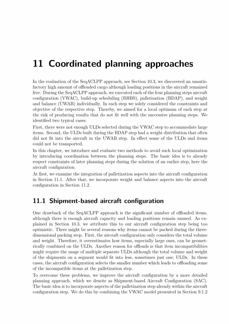
11 Coordinated planning approachesIn the evaluation of the SeqACLPP approach, see Section 10.3, we discovered an unsatis-factory high amount of offloaded cargo although loading positions in the aircraft remainedfree. During the SeqACLPP approach, we executed each of the four planning steps aircraftconfiguration (VWAC), build-up scheduling (RHBS), palletization (BDAP), and weightand balance (UWAB) individually. In each step we solely considered the constraints andobjective of the respective step. Thereby, we aimed for a local optimum of each step atthe risk of producing results that do not fit well with the successive planning steps. Weidentified two typical cases.First, there were not enough ULDs selected during the VWAC step to accommodate largeitems. Second, the ULDs built during the BDAP step had a weight distribution that oftendid not fit into the aircraft in the UWAB step. In effect some of the ULDs and itemscould not be transported.In this chapter, we introduce and evaluate two methods to avoid such local optimizationby introducing coordination between the planning steps. The basic idea is to alreadyrespect constraints of later planning steps during the solution of an earlier step, here theaircraft configuration.At first, we examine the integration of palletization aspects into the aircraft configurationin Section 11.1. After that, we incorporate weight and balance aspects into the aircraftconfiguration in Section 11.2.
11.1 Shipment-based aircraft configurationOne drawback of the SeqACLPP approach is the significant number of offloaded items,although there is enough aircraft capacity and loading positions remain unused. As ex-plained in Section 10.3, we attribute this to our aircraft configuration step being toooptimistic. There might be several reasons why items cannot be packed during the three-dimensional packing step. First, the aircraft configuration only considers the total volumeand weight. Therefore, it overestimates how items, especially large ones, can be geomet-rically combined on the ULDs. Another reason for offloads is that item incompatibilitiesmight require the usage of multiple separate ULDs although the total volume and weightof the shipments on a segment would fit into less, sometimes just one, ULDs. In thesecases, the aircraft configuration selects the smaller number which leads to offloading someof the incompatible items at the palletization step.To overcome these problems, we improve the aircraft configuration by a more detailedplanning approach, which we denote as Shipment-based Aircraft Configuration (SAC).The basic idea is to incorporate aspects of the palletization step already within the aircraftconfiguration step. We do this by combining the VWAC model presented in Section 9.1.2

11 Coordinated planning approaches
A-base A-high A-fast B-base B-high B-fastWLF 0.495 0.971 0.499 0.505 0.961 0.507GLF 0.322 0.683 0.322 0.346 0.688 0.346NLF 0.665 0.708 0.666 0.665 0.703 0.662UNITS 16.090 32.157 16.056 16.915 34.439 16.890SPLIT 0.208 0.263 0.212 0.204 0.276 0.195DISP 2.569 2.940 2.578 2.578 2.941 2.584MIX 0.086 0.112 0.106 0.095 0.155 0.099CREWS 216 415 227 225 409 283
Table 11.1: Performance of SeqACLPP-SAC across all scenarios
A-base A-high A-fast B-base B-high B-fast ∅
WLF 0.406 0.206 1.423 0.798 -0.518 0.198 0.419GLF 0.000 0.441 0.000 0.000 2.381 0.000 0.470NLF 0.453 -0.141 -0.299 0.151 1.151 0.151 0.244UNITS 2.582 0.951 2.877 1.990 5.807 0.578 2.464SPLIT 3.483 1.544 0.952 -0.971 7.812 -1.515 1.884DISP -0.619 -0.877 0.940 1.019 3.229 0.272 0.661MIX -25.862 -5.882 -10.924 -18.803 9.929 -20.161 -11.950CREWS 2.370 1.220 0.000 4.651 4.604 2.536 2.564
Table 11.2: Performance improvement of SeqACLPP-SAC compared to SeqACLPP
and the BinAssign model presented in Section 9.3.1. The objective stays the same as in theoriginal aircraft configuration step, but the added constraints of the bin assignment mustbe fulfilled. By doing this we still do not create three-dimensional load plans during theSAC. The items are only assigned to a ULD considering the ULD capacity, required ULDtypes, and item incompatibilities. Thereby, we expect to get a more realistic estimate ofthe number of required ULDs.Besides the aircraft configuration step, all other steps remain the same as in the SeqA-CLPP approach, presented in Chapter 9. In particular, during palletization items mustnot be packed into the same ULD to which they were assigned by the SAC model. In thefollowing we denote the SeqACLPP approach with the new SAC aircraft configurationstep as SeqACLPP-SAC.
Evaluation
To evaluate the SeqACLPP-SAC approach, we repeated the experiments introduced inSection 10.3. We give an overview of the absolute performance indicators achieved inTable 11.1 and their relative deviation compared to the SeqACLPP approach in Table 11.2.There are only minor variations in the utilization indicators. Most notably, the number ofbuilt ULDs (UNITS) increased by 2.5 percent across all scenarios. However, this does notmean that the ULD capacity increased. More often, PMC ULDs were replaced by multiple
140
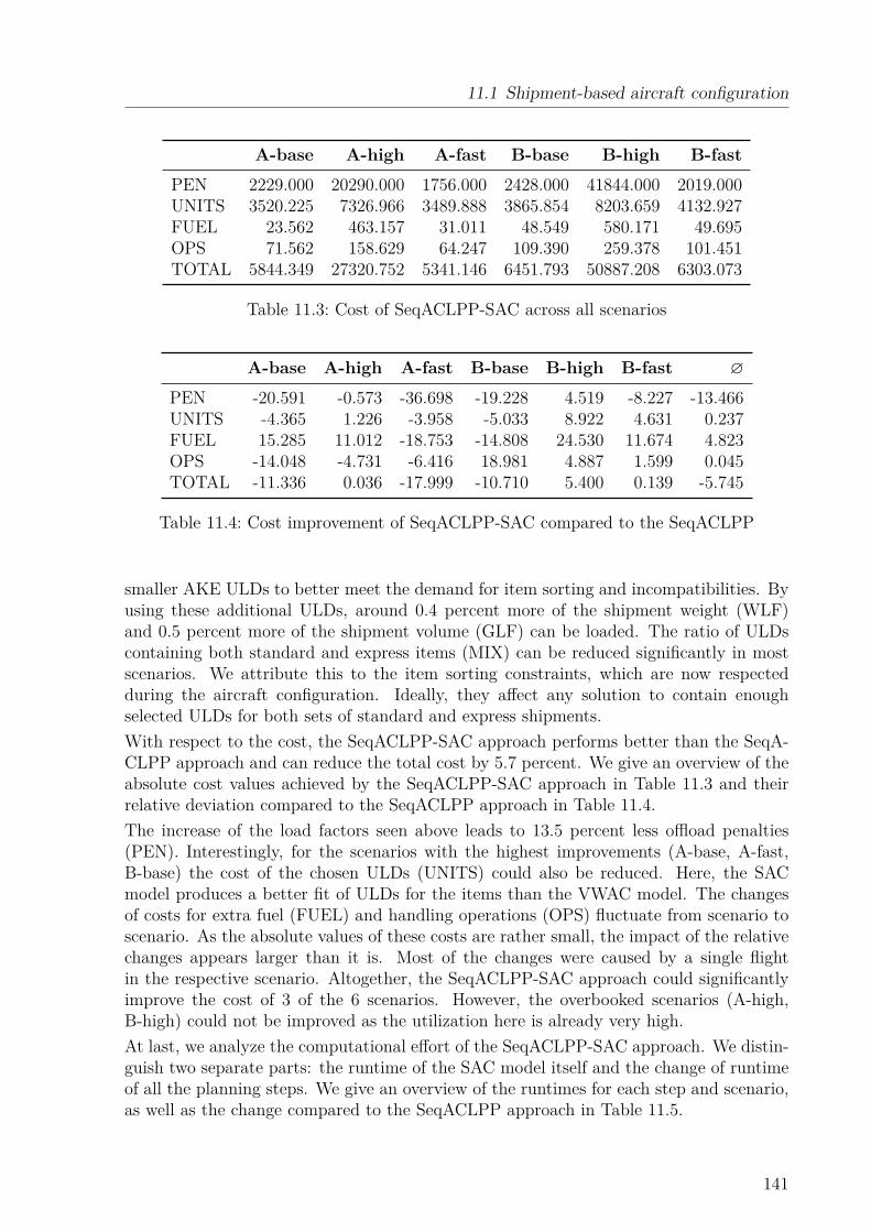
11.1 Shipment-based aircraft configuration
A-base A-high A-fast B-base B-high B-fastPEN 2229.000 20290.000 1756.000 2428.000 41844.000 2019.000UNITS 3520.225 7326.966 3489.888 3865.854 8203.659 4132.927FUEL 23.562 463.157 31.011 48.549 580.171 49.695OPS 71.562 158.629 64.247 109.390 259.378 101.451TOTAL 5844.349 27320.752 5341.146 6451.793 50887.208 6303.073
Table 11.3: Cost of SeqACLPP-SAC across all scenarios
A-base A-high A-fast B-base B-high B-fast ∅
PEN -20.591 -0.573 -36.698 -19.228 4.519 -8.227 -13.466UNITS -4.365 1.226 -3.958 -5.033 8.922 4.631 0.237FUEL 15.285 11.012 -18.753 -14.808 24.530 11.674 4.823OPS -14.048 -4.731 -6.416 18.981 4.887 1.599 0.045TOTAL -11.336 0.036 -17.999 -10.710 5.400 0.139 -5.745
Table 11.4: Cost improvement of SeqACLPP-SAC compared to the SeqACLPP
smaller AKE ULDs to better meet the demand for item sorting and incompatibilities. Byusing these additional ULDs, around 0.4 percent more of the shipment weight (WLF)and 0.5 percent more of the shipment volume (GLF) can be loaded. The ratio of ULDscontaining both standard and express items (MIX) can be reduced significantly in mostscenarios. We attribute this to the item sorting constraints, which are now respectedduring the aircraft configuration. Ideally, they affect any solution to contain enoughselected ULDs for both sets of standard and express shipments.With respect to the cost, the SeqACLPP-SAC approach performs better than the SeqA-CLPP approach and can reduce the total cost by 5.7 percent. We give an overview of theabsolute cost values achieved by the SeqACLPP-SAC approach in Table 11.3 and theirrelative deviation compared to the SeqACLPP approach in Table 11.4.The increase of the load factors seen above leads to 13.5 percent less offload penalties(PEN). Interestingly, for the scenarios with the highest improvements (A-base, A-fast,B-base) the cost of the chosen ULDs (UNITS) could also be reduced. Here, the SACmodel produces a better fit of ULDs for the items than the VWAC model. The changesof costs for extra fuel (FUEL) and handling operations (OPS) fluctuate from scenario toscenario. As the absolute values of these costs are rather small, the impact of the relativechanges appears larger than it is. Most of the changes were caused by a single flightin the respective scenario. Altogether, the SeqACLPP-SAC approach could significantlyimprove the cost of 3 of the 6 scenarios. However, the overbooked scenarios (A-high,B-high) could not be improved as the utilization here is already very high.At last, we analyze the computational effort of the SeqACLPP-SAC approach. We distin-guish two separate parts: the runtime of the SAC model itself and the change of runtimeof all the planning steps. We give an overview of the runtimes for each step and scenario,as well as the change compared to the SeqACLPP approach in Table 11.5.
141

11 Coordinated planning approaches
5% 10% 15% 20% 25% 30% >30%
shar
e of
inst
ance
s [in
%]
010
2030
4050
31.1
46.3
13.4
4.73.2
0.3 0.9
Figure 11.1: SAC MIP gap distribution after 30 seconds runtime (rounded up)
A-base A-high A-fast B-base B-high B-fast ∅ ∆SAC [sec] 26 30 26 28 30 28 28 +∞BDAP [sec] 825 1,991 805 740 2,029 745 1,189 -2.4%UWAB [sec] 47 72 56 66 117 65 71 +16.4%Total [sec] 898 2,093 887 834 2,176 838 1,288 +0.8%
Table 11.5: Computational effort of SeqACLPP-SAC across all scenarios
142

11.2 Weight-and-balance-based aircraft configuration
The runtime of the VWAC model, which we presented in Section 9.1, was negligible. Foralmost all flights, the model solved in well under a second. The SAC model on the otherhand takes much longer to be solved to optimality. Therefore, we stop the MIP searchafter 30 seconds. Around 10 percent of the instances can be solved down to a 1 percentMIP gap until the time limit is reached. The distribution of the resulting MIP gaps ofthe remaining flights is shown in Figure 11.1. Of those flights about 90 percent can besolved with a MIP gap of less than 15 percent.The computational effort required to solve the palletization (BDAP) and weight andbalance (UWAB) steps does not change substantially. The number of LBBD iterationsduring palletization slightly changes for each scenario but on average it stays the same.The average runtime across all scenarios increases by 0.8 percent, a deviation well withinmeasuring tolerance.Accordingly, we can say that the incorporation of palletization aspects into the aircraftconfiguration step works and can be done with acceptable computational effort, albeit itseffects on solution quality are limited.
11.2 Weight-and-balance-based aircraft configuration
The second reason for offloaded items in the SeqACLPP approach, which we identified inSection 10.3, is the offloading of ULDs in the weight and balance step. In the palletizationstep highly utilized and heavy ULDs are created, but afterwards they cannot be loadedinto the aircraft during the weight and balance step. The reason are the cumulativeweight limits of adjacent loading positions, which are not taken into consideration in thefirst three planning steps as no loading positions for the ULDs are assigned yet. Duringpalletization we calculate solutions for each transport segment individually. Therefore,the number and weight distribution of the ULDs of other transport segments on the sameflight is not known during the palletization step for a segment. Consequently, some heavyULDs might be built for each segment.To be able to build ULDs of different segments with a more suitable weight distribution,we present another extension of the aircraft configuration, which we denote as Weight-and-balance-based Aircraft Configuration (WAC). The basic idea is to allot a loading positionand choose a target weight for each ULD already during the aircraft configuration step.Then, in the palletization step exceeding the selected target weight will be penalized.Technically, we create the aircraft configuration by solving a simplification of the weightand balance model (WBM), which we presented in Section 9.4.2. To keep the modelsimple, we only consider the first leg of the flight. This is reasonable, because we expectthat for all ULDs, which are loadable on the first leg, it is possible to find a feasibleloading position on subsequent legs. Furthermore, we omit all aspects modeling reloadingoperations. The model decides for each loading position of the aircraft, for which transportsegment it is used and how much weight should be placed on it. Thereby, we expect toreceive a realistic set of selected ULDs with target weights that can be loaded in theweight and balance step.Table 11.6 introduces the parameters specific to the WAC model. All other parametershave been introduced in Tables 9.2 and 9.11. The model decides about the weight wp,k
143

11 Coordinated planning approaches
Set/Parameter Descriptioncapwgtp ∈ R≥0 weight capacity at loading position pcapvolp ∈ R≥0 volume capacity at loading position pcostp ∈ R handling cost for a ULD on loading position p
Table 11.6: New parameters of the WAC model
placed on loading position p by transport segment k. Besides, auxiliary variables existcapturing the transport segment that is placed on a loading position (xp,k), if a loadingposition is used at all (xp), and what amount of weight is placed on a loading positionirrespective of the transport segment (wp).We formally define the WAC model as follows:
minimize∑k∈K
12y
wgtk offloadwgtk + 1
2yvolk offloadvolk +
∑p∈P
xpcostp
+ fuel+l (11.1)
subject to
demwgtk =
∑p∈P
wp,k + ywgtk k ∈ K (11.2)
demvolk ≤
∑p∈P
xp,kcapvolp + yvolk k ∈ K (11.3)
xp =∑k∈K
xp,k p ∈ P (11.4)
1 ≥ xp + xp′ 〈p, p′〉 ∈ O (11.5)xp ≤
∑p′∈Rp
xp′ p ∈ P (11.6)
wp,k ≤ xp,kcapwgtp p ∈ P (11.7)wp =
∑k∈K
wp,k p ∈ P (11.8)
MAXl ≥∑p∈P
wp (11.9)
limitn ≥∑p∈P
fn,pwp n ∈ N (11.10)
ml = BAacwOEW + BAfuell FWl +
∑p∈P
BAlngp wp (11.11)
wl = wOEW + FWl +∑p∈P
wp (11.12)
Equations (9.101) to (9.107) to calculate fuel+l (11.13)
xp;xp,k ∈ {0, 1} (11.14)ywgtk ; yvolk ;wp;wp,k ∈ R≥0 (11.15)
The objective, given in Equation (11.1), minimizes the total cost from the penalties ofoffloaded cargo weight and volume, the used ULDs, and the extra fuel cost caused by
144

11.2 Weight-and-balance-based aircraft configuration
a suboptimal center of gravity (CG) of the aircraft. Equations (11.2) and (11.3) makesure that the segment demand weight and volume is distributed onto the loading posi-tions or is marked as offloaded. Equation (11.4) marks a loading position if it is used forany transport segment. Mutual exclusions of overlapping loading positions are enforcedby Equation (11.5). The usage order of interdependent loading positions is respectedby Equation (11.6). Equation (11.7) enforces that weight is only placed on used load-ing positions and that the individual weight limit of each loading position is respected.Equation (11.8) collects the weight on each loading position irrespective of the allot-ted transport segment. Equation (11.9) limits the total weight loaded into the aircraft.Equation (11.10) ensures that the cumulative weight limits of the loading positions hold.Equations (11.11) and (11.12) calculate the longitudinal balance arm and the total weightof the loaded aircraft. Both values are input variables for Equations (9.101) to (9.107) tocalculate the extra fuel required due to a suboptimal CG of the loaded aircraft.After the aircraft configuration step, we insert the chosen ULD weights as target weightsfor the ULDs to build during the palletization step. Therefore, we add a target weightparameter targetu for each selected ULD u. Given this parameter, we add the followingconstraint to the BinAssign model from Section 9.3.1 to calculate the excess weight devufor each ULD u:
targetu ≥∑i∈I
weightgrsi assignu,i − devu u ∈ U (11.16)
We do not consider negative deviations, i.e., when the ULD is too light. First, becauseit would generally not limit the loadability of the ULD. Second, these cases already leadto penalties at other parts of the model. If a ULD weight is lower than the target weightbut the same amount of total weight is transported on all ULDs, then another ULD willbe heavier than its target weight and incur penalty cost. Or, if a ULD weight is lowerthan the target weight because some items are offloaded, this also leads to offload penaltycost.At last, we add the deviation from the target weight as cost to the objective of the binassignment model:
Equation (9.28) + α∑u∈U
dev2u (11.17)
In our actual implementation we approximated the penalty by a piecewise linear functionin steps of 100 kg. Furthermore, we add a factor α to weight the total penalty of targetweight deviations because it can not be directly translated into cost. Weighting thedeviations too high would lead to offloads during the palletization step although moreweight could be loaded into the aircraft. On the other hand, if the deviations are weightedtoo low, it becomes easy for the model to disregard the target weights. In our experimentswe set α to 0.01, which produced reasonable results.Let BDAP+ denote the updated palletization step, i.e., where the BinAssign model isextended by Equations (11.16) and (11.17). The build-up scheduling (RHBS) and weightand balance (UWAB) steps remain the same as in the SeqACLPP approach, presentedin Chapter 9. In the following we denote the SeqACLPP approach with the new WACaircraft configuration step as SeqACLPP-WAC.
145

11 Coordinated planning approaches
A-base A-high A-fast B-base B-high B-fastWLF 0.509 0.919 0.513 0.514 0.934 0.517GLF 0.322 0.639 0.322 0.346 0.650 0.346NLF 0.655 0.676 0.658 0.661 0.689 0.656UNITS 16.090 34.787 16.067 17.110 34.354 17.354SPLIT 0.274 0.287 0.266 0.277 0.297 0.285DISP 2.647 3.035 2.658 2.640 3.026 2.633MIX 0.123 0.095 0.130 0.139 0.176 0.140CREWS 215 428 231 216 403 272
Table 11.7: Performance of SeqACLPP-WAC across all scenarios
A-base A-high A-fast B-base B-high B-fast ∅
WLF 3.245 -5.160 4.268 2.595 -3.313 2.174 0.635GLF 0.000 -6.029 0.000 0.000 -3.274 0.000 -1.550NLF -1.057 -4.654 -1.497 -0.452 -0.863 -0.756 -1.546UNITS 2.582 9.208 2.947 3.166 5.545 3.341 4.465SPLIT 36.318 10.811 26.667 34.466 16.016 43.939 28.036DISP 2.398 2.326 4.072 3.448 6.213 2.173 3.438MIX 6.034 -20.168 9.244 18.803 24.823 12.903 8.607CREWS 1.896 4.390 1.762 0.465 3.069 -1.449 1.689
Table 11.8: Performance improvement of SeqACLPP-WAC compared to SeqACLPP
Evaluation
To evaluate the SeqACLPP-WAC approach, we repeated the experiments introduced inSection 10.3. We follow the same evaluation scheme as used in Section 11.1 for theShipment-based Aircraft Configuration. We give an overview of the absolute performanceindicators achieved in Table 11.7 and their relative deviation compared to the SeqACLPPapproach in Table 11.8.With respect to the solution quality, we get a heavily diverging picture for the base andfast scenarios on one side and the high scenarios on the other. The weight load factor(WLF) can be improved in all base and fast scenarios, on average by more than 3 percent.However, the WLF decreases in the high scenarios by 4.2 percent. For these overbookedflights, the WAC seems to be too conservative, when assigning weight to the ULDs. Theaim of the WAC is the creation of loadable ULD target weights that result in a wellbalanced aircraft, but in these cases balancing should not the prime concern. Also thevolume net load factor (NLF) reduces across all scenarios by around 1.5 percent while4.5 percent more ULDs are built (UNITS). However, this is reasonable, as the chosentarget weights are often significantly below the weight limit of a ULD type and thus theload needs to be split across more ULDs. This also has a negative impact on the handlingindicators. The share of shipments that are split (SPLIT) increases significantly in allscenarios, on average by 28 percent. The increase of dispersion of splitted shipments
146

11.2 Weight-and-balance-based aircraft configuration
A-base A-high A-fast B-base B-high B-fastPEN 958.000 27786.000 598.000 586.000 47863.000 405.000UNITS 3844.944 7575.281 3851.685 4278.049 7991.463 4014.634FUEL 13.933 390.225 11.449 18.927 429.220 19.341OPS 64.258 146.067 62.809 76.098 236.220 64.976TOTAL 4881.135 34979.573 4523.943 4960.074 56519.903 4503.951
Table 11.9: Cost of SeqACLPP-WAC across all scenarios
A-base A-high A-fast B-base B-high B-fast ∅
PEN -65.871 36.159 -78.443 -80.506 19.553 -81.591 -41.783UNITS 4.457 4.657 5.999 5.093 6.104 1.636 4.658FUEL -31.828 -6.469 -70.004 -66.788 -7.871 -56.537 -39.916OPS -22.821 -12.275 -8.511 -17.230 -4.478 -34.929 -16.707TOTAL -25.949 28.079 -30.545 -31.355 17.067 -28.445 -11.858
Table 11.10: Cost improvement of SeqACLPP-WAC compared to SeqACLPP
(DISP) by 3.4 percent and share of ULDs with both standard and express shipments(MIX) by 8.6 percent is also noticeable albeit less drastic.In the base and fast scenarios the disadvantage of a higher handling effort is compensatedby a significant reduction of most cost components. On average the penalties for offloadeditems can be reduced by more than 76 percent in those scenarios. The bad performanceof the WAC for the high scenarios also shows in the penalty cost, which are 27.9 percenthigher than in the SeqACLPP approach. The cost for built ULDs increases across allscenarios. This effect is in line with the rise in the number of used ULDs. The costfor extra fuel due to imbalances (FUEL) can be reduced by 39.9 percent and handlingoperations (OPS) by 16.7 percent from their already low absolute levels. Thus, in the baseand fast scenario an almost ideal balance can be achieved for most of the flights, whilethe number of performed reloading operations is less than one ULD per flight on average.Altogether, the total cost for flights in the base and fast scenarios could be reduced bymore than 29 percent compared to the SeqACLPP approach. But, for highly bookedflights the total cost is around 22.6 percent higher than in the SeqACLPP approach, dueto the increased offloads. Therefore, it seems beneficial to choose the concrete solutionapproach on a flight-per-flight basis, depending on the respective utilization.At last, we analyze the runtime of the WAC approach. As in the last section, we firstlook at the runtime of the WAC model itself. After that, we discuss the impact on theruntime of the other planning steps.Similar to the SAC model, the WAC model takes a noticeable amount of time to be solvedto optimality for most flights. Therefore, we also set a time limit of 30 seconds for theaircraft configuration step. Around 50 percent of the flights can be solved down to a1 percent MIP gap until this time limit is reached. The distribution of the resulting MIPgaps of the remaining flights is shown in Figure 11.2. Almost all of those flights show aMIP gap of less than 10 percent.
147
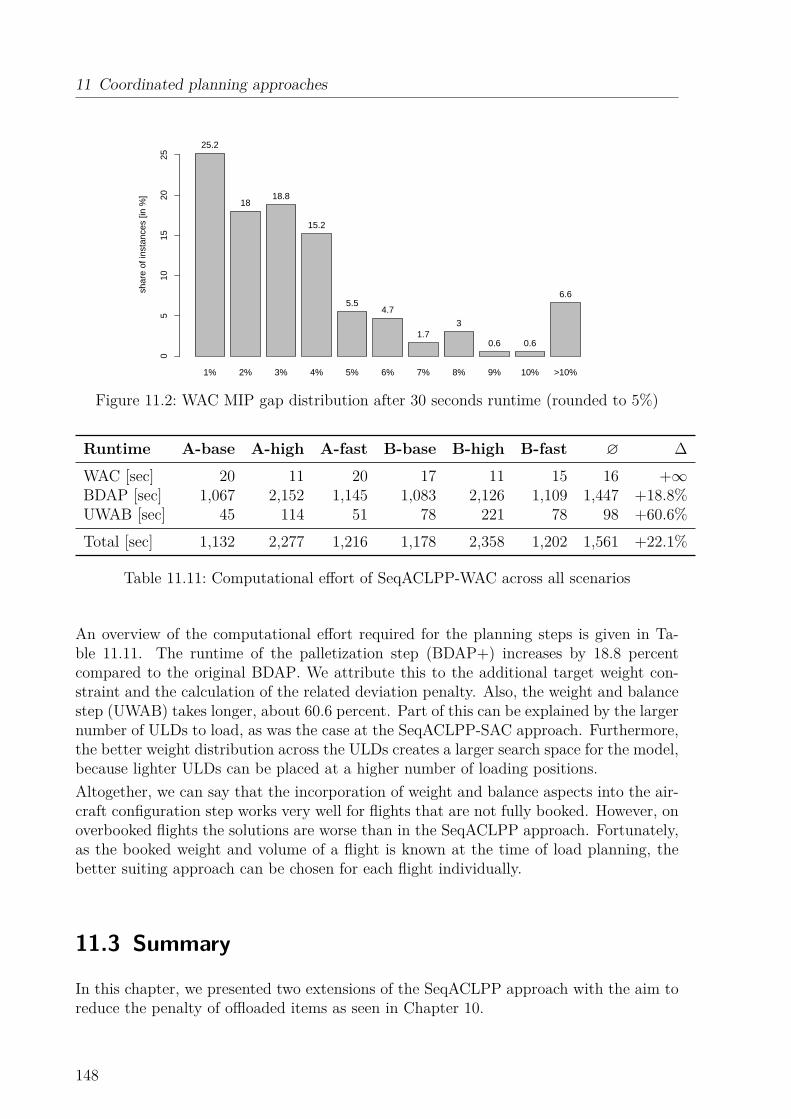
11 Coordinated planning approaches
1% 2% 3% 4% 5% 6% 7% 8% 9% 10% >10%
shar
e of
inst
ance
s [in
%]
05
1015
2025
25.2
1818.8
15.2
5.54.7
1.73
0.6 0.6
6.6
Figure 11.2: WAC MIP gap distribution after 30 seconds runtime (rounded to 5%)
Runtime A-base A-high A-fast B-base B-high B-fast ∅ ∆WAC [sec] 20 11 20 17 11 15 16 +∞BDAP [sec] 1,067 2,152 1,145 1,083 2,126 1,109 1,447 +18.8%UWAB [sec] 45 114 51 78 221 78 98 +60.6%Total [sec] 1,132 2,277 1,216 1,178 2,358 1,202 1,561 +22.1%
Table 11.11: Computational effort of SeqACLPP-WAC across all scenarios
An overview of the computational effort required for the planning steps is given in Ta-ble 11.11. The runtime of the palletization step (BDAP+) increases by 18.8 percentcompared to the original BDAP. We attribute this to the additional target weight con-straint and the calculation of the related deviation penalty. Also, the weight and balancestep (UWAB) takes longer, about 60.6 percent. Part of this can be explained by the largernumber of ULDs to load, as was the case at the SeqACLPP-SAC approach. Furthermore,the better weight distribution across the ULDs creates a larger search space for the model,because lighter ULDs can be placed at a higher number of loading positions.Altogether, we can say that the incorporation of weight and balance aspects into the air-craft configuration step works very well for flights that are not fully booked. However, onoverbooked flights the solutions are worse than in the SeqACLPP approach. Fortunately,as the booked weight and volume of a flight is known at the time of load planning, thebetter suiting approach can be chosen for each flight individually.
11.3 Summary
In this chapter, we presented two extensions of the SeqACLPP approach with the aim toreduce the penalty of offloaded items as seen in Chapter 10.
148

11.3 Summary
In our first extension, denoted as Shipment-based Aircraft Configuration (SeqACLPP-SAC), we integrated the non-geometric aspects of the palletization step into the aircraftconfiguration step. Besides selecting the ULDs, the model also assigns items to ULDs.Thereby, it obtains a more detailed view of the problem that results in a more suitable setof selected ULDs. Across all scenarios, this approach could reduce the penalty of offloadeditems (PEN) by 13.5 percent. This resulted in a reduction of the total cost by 5.7 percent.The increased load resulted in about 2.5 percent more ULDs to be built (UNITS) andthe intended separation of items (MIX) could be improved by 12 percent. Besides, thesolution quality and runtime showed no significant changes to the SeqACLPP approach.The second extension, denoted as Weight-and-balance-based Aircraft Configuration (Se-qACLPP-WAC), integrates weight and balance aspects like the weight distribution andstructural aircraft limits into the aircraft configuration step. Besides the ULD selection,each ULD is now assigned to a loading position and given a target weight. If the targetweights are met during the palletization step, all ULDs are loadable and lead to a goodaircraft balance. Therefore, we also extended the palletization step, to respect the tar-get weights as a soft constraint. This approach worked very well for the base and fastscenarios. Over all scenarios the penalties of offloaded items (PEN) could be reduced by41.8 percent and resulted in 4.7 percent more ULDs (UNITS) to be built. The cost foradditional fuel due to imbalance (FUEL) could be significantly reduced by 39.9 percent.Furthermore, the cost of reloading operations (OPS) could be reduced by 16.7 percent.This led to a reduction of total costs by 29 percent across the base and fast scenarios. How-ever, over all scenarios the total cost improvement was only 11.9 percent, as the approachdid not produce good results for the high-load scenarios. Here, on average 4.2 percentless weight could be loaded per flight. In this case, the new model focuses too much oncheap aircraft operations, which is not the prime concern on the highly utilized flights.Altogether, we find that a coordination of the planning steps seems to be a promisingway to improve solution quality with reasonable implementation and computational effort.While the proposed extensions work well for ordinary utilized flights, for highly bookedflights the SeqACLPP approach should be preferred.
149


12 Conclusion
In this chapter, we summarize the main contributions and results of this thesis. Wediscuss our findings regarding the stated research questions and conclude with an outlookon promising future research.
12.1 Summary
The goal of this work was to understand the load planning problem faced by cargo airlinesand develop suitable solution approaches by using operations research methods to createa decision support system. Along this way, we generated several contributions to thestate of research, which we introduce in the following in the order of their appearance inthis thesis. Besides, we give a graphical overview of the developed models and solutionapproaches in Figure 12.1.In Chapter 2, we presented a brief introduction into the air cargo business as well asthe operational handling processes of airlines that transport cargo. After that, we gavea comprehensive overview of the Air Cargo Load Planning Problem (ACLPP) and itsfour subproblems: the Aircraft Configuration Problem (ACP), the Build-up SchedulingProblem (BSP), the Air Cargo Palletization Problem (APP), and the Weight and BalanceProblem (WBP) in Chapter 3. We identified the three main stakeholders of load planning:sales, handling, and aircraft operations. Their respective objectives on the problem aremaximizing revenue, minimizing physical handling effort, and minimizing operationalcost of the flight. Furthermore, we discussed the challenges of current manual planningapproaches.In the next four Chapters 4 to 7 we introduced the ACLPP subproblems one by one indetail. For each subproblem, we reviewed the existing literature and formally specified anoptimization model (ACM, BSM, APM, WBM). The ACM and BSM are the first modelstackling the respective problems. For the APP and WBP only models partially coveringthe aspects of our problem at hand could be found. The APM especially introduces thefollowing features that have not yet been dealt with in the literature:• It considers time as a new dimension of the packing problem. Only items that are
available before the assembly time of a ULD can be assigned to it.• The stacking and stability constraints track the statics between the items and allow
for partial support as well as placement on uneven surfaces.• To cover item allocation restrictions, a soft item sorting constraint is added. It
allows for groups of items to be packed preferably together or onto separate ULDs.In the WBM we consider the union of constraints found in the literature. Besides, weadded the following practical aspects:

12 Conclusion
Problem / Model
Aircraft configurationACP / ACM (4.2)
Build-up schedulingBSP / BSM (5.2)
Air cargo palletizationAPP / APM (6.2)
Weight and balanceWBP / WBM (7.2)
ACLP
PSolution
VWAC (9.1)
RHBS (9.2)
BDAP (9.3)
UWAB (9.4)
SeqA
CLP
P(9)
Extensions
SeqA
CLP
P-SAC
(11.1) SAC
RHBS
BDAP
UWAB
SeqA
CLP
P-W
AC
(11.2) WAC
RHBS
BDAP+
UWAB
Figure 12.1: Components presented in this work, along with the sections they are intro-duced in.
• The formulation accommodates an arbitrary number of flight legs.• A new dependency constraint is added that forces certain loading positions to be
occupied to be allowed to use other dependent positions.• A variety of formulations of cumulative load constraints have been presented in the
literature. In our formulation, one standardized constraint is present that handlesall cumulative weight limits with maximum flexibility.
To evaluate solution approaches to the ACLPP, we introduced a set of benchmark in-stances in Chapter 8. Therefore, we created a data model covering all the consideredaircraft and ULD characteristics, regulatory requirements, and booking data. Further-more, we presented an analysis of real world air cargo booking data to grasp the problemstructure and planning difficulties. We found that the flights are often not fully booked.Accordingly, dense packing is not always the prime objective and planning results thatlead to efficient handling as well as aircraft operations are also highly important. Theitems to be loaded are strongly heterogeneous in their dimensions, weight, and densityand a significant part of the items is quite large, often exceeding the size of a standardwooden pallet. We introduced two benchmark datasets, one non-public set based on realflight data and a public set created by us that contains sampled booking data. Fromboth sets we generated two additional scenarios of use cases that are interesting from apractical point of view. The first contains only overbooked flights and in the other thebookings have shorter transfer times at the terminal. From the public dataset, we providea dataset of 246 realistic flights for future research.To solve the ACLPP in practice, we designed and implemented a decision support system.Its details are presented in Chapter 9. Our approach, denoted as SeqACLPP, consists
152

12.2 Research questions
of a sequential four-step planning pipeline that follows the current manual processes inpractice. The ACP is solved for each flight by a MIP model implementing a Weight-and-Volume-based Aircraft Configuration (VWAC). For the BSP we presented a rollinghorizon approach (RHBS) considering all flights in the planning horizon. It solves one shiftper iteration by also employing a MIP model. We realized the APP with a Logic-basedBenders Decomposition approach, denoted as BDAP, which is solved for each transportsegment of a flight. It consists of a MIP master problem and subproblems solved via aconstraint program. The master problem, denoted as BinAssign, distributes the itemsamong the ULDs and covers all non-geometric aspects of the problem. The subproblem,denoted as CPPack, captures all the three-dimensional packing aspects. Finally, the WBPis solved for each flight by a MIP model, denoted as ULD-based Weight and Balance(UWAB).We successfully evaluated the SeqACLPP approach on the introduced benchmark in-stances and reported the results in Chapter 10. As the approach contains a number ofparameters, we introduced a set of methods to determine suitable settings. Furthermore,we discussed the achieved results with respect to solution quality and effort and identifiedareas for improvement.Based on identified weaknesses of the SeqACLPP approach, we introduced and evaluatedtwo coordinated planning approaches in Chapter 11. In the SeqACLPP-SAC approachwe incorporate aspects of the APP into the ACP by replacing the VWAC with a newShipment-based Aircraft Configuration (SAC). In the same way, in the SeqACLPP-WACapproach we replace the VWAC with a Weight-and-balance-based Aircraft Configuration(WAC) to consider WBP aspects within the ACP step. Finally, we analyzed the effectsof both approaches on the solution quality and runtimes. Both approaches can furtherimprove the solutions.
12.2 Research questionsIn this work, we followed three research questions introduced in Section 1.2. As indicatedin the previous summary section we found satisfactory answers to all of them. In thefollowing, we give a brief statement of the results and point out the parts of this workwhere detailed information can be found.
1) What are the requirements and drivers of air cargo load planning in practice?The ACLPP affects three airline departments: sales, handling, and aircraft operations.All three have partially conflicting objectives on the subject. We identified four parts ofthe problem: aircraft configuration, build-up scheduling, palletization, and weight andbalance. After introducing the general planning process in Chapter 3, we described thefour parts in detail and formally in Chapters 4 to 7.
2) Can valid and competitive load plans be generated with reasonable effort? Fromthe identified parts of the problem, we derived the four-step planning approach SeqA-CLPP. We implemented it and evaluated its performance on real and synthetic benchmarkinstances. Compared to real load plans seen in practice, the average packing density could
153

12 Conclusion
be improved by more than 20 percent and the performance with respect to the requiredhandling effort and aircraft operations could be significantly improved. The required run-times range between 13 and 38 minutes per flight, which is acceptable for non-interactiveplanning. We described our solution approach in Chapter 9 and its evaluation in Chap-ter 10.
3) Does splitting the problem lead to adverse effects and what can we do aboutit? During the evaluation of the SeqACLPP approach we found that considering eachsolution step independently leads to a higher than necessary amount of offloaded items.The reason typically is an overestimation of the capabilities of later steps. For example,the volume capacity of a single ULD is easily overestimated if only the volume of theitems to be loaded is considered. Furthermore, the aircraft capacity for heavy ULDs isoverestimated if only a subset of the ULDs to load is considered. To overcome thoseeffects, we incorporated constraints of later planning steps into the aircraft configurationstep. Thereby, we could improve the solution quality for four out of six scenarios. Thesecoordinated planning approaches are presented in detail in Chapter 11.
12.3 Future workThe presented approaches provide numerous opportunities for improvement and futureresearch. Our first set of suggestions targets technical aspects of the presented approaches.During the Logic-based Benders Decomposition of the palletization step (BDAP), theheuristic cuts added in each iteration are not always effective and therefore many iterationsare necessary before the process comes to an end. Here, improved cuts, ideally representingminimal infeasible sets of items, could be advantageous. Especially in the high-loadscenarios, the offloaded items provided many alternatives to bypass the cuts and stillproduce unpackable results. For these cases, a dual perspective for cuts that limit theusable bin capacity might be promising.Furthermore, the runtimes need to be improved to make the solution process interactivelyusable. Besides better cuts, this could be achieved through parallelization or furtherdecomposition of the problems. In the BDAP we decomposed the problem by the volumeof the items. Besides that, the separate planning of express items or dangerous goodsmight be conceivable.The second area for enhancements we identified is to improve the solution quality andreduce the search space by a further integration of the planning steps. Most obvious,the presented coordinated solution approaches, i.e., the shipment-based and weight-and-balance-based aircraft configuration, could be put into one model. Besides that, schedul-ing aspects, like item availability or shortages of the build-up capacity, could be addedto the aircraft configuration. Furthermore, the combined weight limits of the weight andbalance step could be integrated into the palletization step, to provide a more detailedpicture of loadable ULD weights.A third field of future research is the integration of additional practical aspects into themodel. In the palletization step, we introduced a stacking constraint with a certain heighttolerance. In practice the emerging vertical gaps can be filled by using dunnage material
154

12.4 Outlook
if necessary. However, an explicit planning of dunnage material could also be interesting.Especially on lower deck ULDs, where only overhanging items can fill the full contour,a scaffold made of wooden pallets or boards is sometimes used in practice to be able topack more items onto the ULD.Next, during the build-up scheduling we assumed a constant assembly time for eachULD type to keep things simple. However, discussions with practitioners suggest thatthe structure of the items assigned to a ULD also has an impact on the assembly time.Furthermore, it is also occasional practice to assign multiple crews to a ULD build-up tospeed up the process to a certain extent. Incorporating these aspects adds more degreesof freedom to the designed load plans and could therefore improve solution quality.Finally, our model assumed full knowledge of all item properties. Although accurate datais increasingly available, items might always differ from the shippers statement or statedproperties like the load-bearing strength might turn out to be wrong. To cope with suchuncertain data, an idea would be to introduce some kind of Monte Carlo sampling of itemproperties, solve the three-dimensional packing problem for multiple scenarios and onlyaccept solutions with a certain feasibility probability.
12.4 OutlookOur evaluation showed that the presented approaches are suitable to automatically gen-erate load plans for cargo flights. The generated load plans are significantly better thanplans manually created by load planning experts. Compared to the current operationalpractice, we could, for example, achieve a 20 percent higher packing density and reducethe required warehouse to workstation transports in the air cargo terminal by more than17 percent due to better item sorting. The costs of additional fuel burn due to aircraftimbalances or ULD reloading operations at stop-over airports in our solutions are almostnegligible.This shows that cargo airlines can significantly profit from employing the presented ap-proaches in their operational practice. More and especially the profitable last-minutecargo can be transported. Furthermore, the costs of load planning, handling effort, andaircraft operations can be significantly reduced. In the highly competitive air cargo busi-ness this can provide airlines with a competitive edge to operate profitably.Besides the operational load planning, further use cases of the presented approaches areimaginable. They could be used throughout the booking process to estimate the actualaircraft utilization of a flight or to calculate the effective space required by a new booking.On a tactical level new products or routes could be evaluated by exemplary load plan-ning. Even the aircraft can be optimized by simulating the effects of added or removedequipment, like floor locks or additional fuel tanks, on the load plans in practice. Thesechanges modify the aircraft configuration space and hence its loading capabilities, butthey also alter the weight of the unloaded aircraft and thus its fuel consumption on anyflight.
155


BibliographyAmadeus (2015). Amadeus Flight Management. Technical report, Amadeus IT GroupSA. Available online from: www.amadeus.com, last accessed: 18.05.2017.
Bischoff, E. and M. Ratcliff (1995). Issues in the development of approaches to containerloading. Omega 23 (4), p. 377 – 390.
Boeing (2011). MD-11 airplane characteristics for airport planning. Technical report,Boeing Commercial Airplanes. Available online from: www.boeing.com, last accessed:18.05.2017.
Bortfeldt, A. and G. Wäscher (2013). Constraints in container loading: A state-of-the-artreview. European Journal of Operational Research 229 (1), p. 1 – 20.
Brandt, F., J.-N. Popratnjak and E. Schulz (2014, 3). Packing with Item Availability andBin Due Dates. Presentation at the 11th Meeting of the EURO Special Interest Groupon Cutting and Packing.
Brosh, I. (1981). Optimal cargo allocation on board a plane: a sequential linear program-ming approach. European Journal of Operational Research 8 (1), p. 40 – 46.
Burnson, P. (2013). Top 25 Freight Forwarders: Top 25 prevail despite market divergence.Logistics Management. Available online from: www.logisticsmgmt.com, last accessed:18.05.2017.
Ceschia, S. and A. Schaerf (2013). Local search for a multi-drop multi-container loadingproblem. Journal of Heuristics 19 (2), p. 275–294.
Chan, F. T., R. Bhagwat, N. Kumar, M. Tiwari and P. Lam (2006). Development of adecision support system for air-cargo pallets loading problem: A case study. ExpertSystems with Applications 31 (3), p. 472 – 485.
Crabtree, T., T. Hoang, J. Edgar and R. Tom (2014). Boeing World Air Cargo Forecast2014-2015. Technical report, Boeing Commercial Airplanes. Available online from:www.boeing.com, last accessed: 18.05.2017.
Crabtree, T., T. Hoang, R. Tom and G. Gildemann (2016). Boeing World Air CargoForecast 2016-2017. Technical report, Boeing Commercial Airplanes. Available onlinefrom: www.boeing.com, last accessed: 18.05.2017.
Crainic, T. G., G. Perboli and R. Tadei (2008). Extreme Point-Based Heuristics forThree-Dimensional Bin Packing. INFORMS Journal on Computing 20 (3), p. 368–384.
157

Bibliography
Dahmani, N. and S. Krichen (2016). Solving a load balancing problem with a multi-objective particle swarm optimisation approach: application to aircraft cargo trans-portation. International Journal of Operational Research 27 (1-2), p. 62–84.
de Cleyn, S., K. de Vos, T. Kallstenius, E. van Bruystegem, W. van Daele and S. Ver-meulen (2014). Optimization takes flight with weight and balance software for airlines.Technical report, iMinds insights. Available online from: www.iminds.be, last accessed:24.04.2017.
Egeblad, J., C. Garavelli, S. Lisi and D. Pisinger (2010). Heuristics for container loadingof furniture. European Journal of Operational Research 200 (3), p. 881 – 892.
Eley, M. (2003). A bottleneck assignment approach to the multiple container loadingproblem. OR Spectrum 25 (1), p. 45–60.
FAA (2016). Aircraft Weight and Balance Handbook. Technical report, Federal AviationAdministration. Available online from: www.faa.gov, last accessed: 18.05.17.
Feng, B., Y. Li and Z.-J. M. Shen (2015). Air cargo operations: Literature review andcomparison with practices. Transportation Research Part C: Emerging Technologies 56,p. 263 – 280.
Fuellerer, G., K. F. Doerner, R. F. Hartl and M. Iori (2010). Metaheuristics for vehi-cle routing problems with three-dimensional loading constraints. European Journal ofOperational Research 201 (3), p. 751 – 759.
Grandjot, H., I. Roessler and A. Roland (2007). Air Cargo Guide: An Introduction to theAir Cargo Industry. Huss.
Guéret, C., N. Jussien, O. Lhomme, C. Pavageau and C. Prins (2003). Loading Aircraftfor Military Operations. The Journal of the Operational Research Society 54 (5), p.458–465.
Heidelberg, K. R., G. S. Parnell and J. E. Ames (1998). Automated air load planning.Naval Research Logistics (NRL) 45 (8), p. 751–768.
Hodgson, T. J. (1982). A Combined Approach to the Pallet Loading Problem. AIIETransactions 14 (3), p. 175–182.
Hong Ha, H. T. and N. Nananukul (2016). Air Cargo Loading Management Systemfor Logistics Forwarders. In: Proceedings of 2016 International Conference on UrbanPlanning, Transport and Construction Engineering, Pattaya, p. 51–58.
Hooker, J. N. (2007). Planning and Scheduling by Logic-Based Benders Decomposition.Operations Research 55 (3), p. 588–602.
IATA (2016). Dangerous Goods Regulations. International Air Transport Association.Available online from: www.iata.org, last accessed: 18.05.2017.
158

Bibliography
ISO (2003). ISO 6780:2003: Flat pallets for intercontinental materials handling – Principaldimensions and tolerances. Technical report, International Organization for Standard-ization.
Junqueira, L., R. Morabito and D. S. Yamashita (2012). Three-dimensional containerloading models with cargo stability and load bearing constraints. Computers and Op-erations Research 39 (1), p. 74 – 85.
Larsen, O. and G. Mikkelsen (1980). An interactive system for the loading of cargoaircraft. European Journal of Operational Research 4 (6), p. 367 – 373.
Lau, H. C. W., T. M. Chan, W. T. Tsui, G. T. S. Ho and K. L. Choy (2009). An AIapproach for optimizing multi-pallet loading operations. Expert Systems with Applica-tions 36 (3), p. 4296–4312.
Limbourg, S., M. Schyns and G. Laporte (2012). Automatic aircraft cargo load planning.Journal of the Operational Research Society 63 (9), p. 1271–1283.
Lin, J. L., C. H. Chang and J. Y. Yang (2006). A study of optimal system formultiple-constraint multiple-container packing problems. Lecture Notes in ComputerScience 4031 LNAI, p. 1200–1210.
Lurkin, V. and M. Schyns (2015). The Airline Container Loading Problem with pickupand delivery. European Journal of Operational Research 244 (3), p. 955 – 965.
Mongeau, M. and C. Bes (2003). Optimization of aircraft container loading. Aerospaceand Electronic Systems 39 (1), p. 140–150.
Murray, G. (2016). Load factors at historic lows, says IATA. Air Cargo News. Availableonline from: www.aircargonews.net, last accessed: 18.05.2017.
Nance, R., A. Roesener and J. Moore (2011). An advanced tabu search for solvingthe mixed payload airlift loading problem. The Journal of the Operational ResearchSociety 62 (2), p. 337–347.
Nobert, Y. and J. Roy (1998). Freight Handling Personnel Scheduling at Air CargoTerminals. Transportation Science 32 (3), p. 295–301.
Paquay, C., M. Schyns and S. Limbourg (2016). A mixed integer programming formulationfor the three-dimensional bin packing problem deriving from an air cargo application.International Transactions in Operational Research 23 (2), p. 187–213.
Pisinger, D. and M. Sigurd (2007). Using decomposition techniques and constraint pro-gramming for solving the two-dimensional bin-packing problem. INFORMS Journal onComputing 19 (1), p. 36–51.
Pollaris, H., K. Braekers, A. Caris, G. K. Janssens and S. Limbourg (2015). Vehiclerouting problems with loading constraints: state-of-the-art and future directions. ORSpectrum 37 (2), p. 297–330.
159
Bibliography
Rong, A. and M. Grunow (2009). Shift designs for freight handling personnel at air cargoterminals. Transportation Research Part E: Logistics and Transportation Review 45 (5),p. 725 – 739.
Techanitisawad, A. and P. Tangwiwatwong (2004). A GA-based Heuristic for the Inter-related Container Selection Loading Problems. IEMS 3 (1), p. 22–37.
The Economist (2016). Too little freight, too much space. The Economist. Availableonline from: www.economist.com, last accessed: 24.04.2017.
Tyler, T. (2015). IATA Annual Review 2015. Technical report, International Air Trans-port Association. Available online from: www.iata.org, last accessed: 18.05.2017.
Vancroonenburg, W., J. Verstichel, K. Tavernier and G. V. Berghe (2014). Automaticair cargo selection and weight balancing: A mixed integer programming approach.Transportation Research Part E: Logistics and Transportation Review 65, p. 70 – 83.
Wikipedia (2016). Pallet — Wikipedia, The Free Encyclopedia. Available online at:http://en.wikipedia.org/wiki/Pallet, last accessed 31.10.2016.
Wu, Y. (2008). Modelling containerisation of air cargo forwarding problems. ProductionPlanning & Control 19 (1), p. 2–11.
Yan, S., C.-H. Chen and C.-K. Chen (2006a). Long-term manpower supply planning forair cargo terminals. Journal of Air Transport Management 12 (4), p. 175–181.
Yan, S., C.-H. Chen and C.-K. Chen (2008a). Short-term shift setting and manpowersupplying under stochastic demands for air cargo terminals. Transportation 35 (3), p.425–444.
Yan, S., C.-H. Chen and M. Chen (2008b). Stochastic models for air cargo terminal man-power supply planning in long-term operations. Applied Stochastic Models in Businessand Industry 24, p. 261–275.
Yan, S., C. K. Chen and C. H. Chen (2006b). Cargo terminal shift setting and manpowersupplying in short-term operations. Journal of Marine Science and Technology 14 (2),p. 109–118.
Yan, S., C.-T. Lo and Y.-L. Shih (2006). Cargo Container Loading Plan Model andSolution Method for International Air Express Carriers. Transportation Planning andTechnology 29 (6), p. 445–470.
160
List of Figures2.1 Illustration of flights, legs, and segments . . . . . . . . . . . . . . . . . . . 82.2 Images of packed ULDs . . . . . . . . . . . . . . . . . . . . . . . . . . . . . 102.3 Examples of ULD types . . . . . . . . . . . . . . . . . . . . . . . . . . . . 102.4 Air cargo modes of transport . . . . . . . . . . . . . . . . . . . . . . . . . . 112.5 Material flow in an air cargo terminal . . . . . . . . . . . . . . . . . . . . . 132.6 Build-up workstations in a cargo terminal . . . . . . . . . . . . . . . . . . 142.7 Images of aircraft loading . . . . . . . . . . . . . . . . . . . . . . . . . . . 152.8 Deck layout of an MD11F aircraft . . . . . . . . . . . . . . . . . . . . . . . 16
3.1 Load planning stakeholders and objectives . . . . . . . . . . . . . . . . . . 183.2 Workflow of load planning in practice . . . . . . . . . . . . . . . . . . . . . 22
4.1 Example aircraft configuration . . . . . . . . . . . . . . . . . . . . . . . . . 234.2 Alternative configurations inside a compartment . . . . . . . . . . . . . . . 25
5.1 Example build-up demand curve . . . . . . . . . . . . . . . . . . . . . . . . 32
6.1 Modeling of irregular shaped bins . . . . . . . . . . . . . . . . . . . . . . . 466.2 Illustration of the stacking model . . . . . . . . . . . . . . . . . . . . . . . 49
7.1 Illustration of the aircraft center of gravity . . . . . . . . . . . . . . . . . . 65
8.1 ACLPP data model . . . . . . . . . . . . . . . . . . . . . . . . . . . . . . . 728.2 Distribution of the number of legs per flight . . . . . . . . . . . . . . . . . 748.3 Distribution of weight utilization among flights (in %) . . . . . . . . . . . . 748.4 Distribution of volume utilization on flights (in %) . . . . . . . . . . . . . . 758.5 Distribution of the number of items per segment . . . . . . . . . . . . . . . 758.6 Distribution of the number of item groups per shipment . . . . . . . . . . . 768.7 Distribution of item frequencies in all shipments . . . . . . . . . . . . . . . 778.8 Distribution of item lengths . . . . . . . . . . . . . . . . . . . . . . . . . . 778.9 Distribution of item widths . . . . . . . . . . . . . . . . . . . . . . . . . . 788.10 Distribution of width-to-length aspect ratio . . . . . . . . . . . . . . . . . . 788.11 Distribution of item heights . . . . . . . . . . . . . . . . . . . . . . . . . . 798.12 Distribution of height-to-length aspect ratio . . . . . . . . . . . . . . . . . 808.13 Distribution of item density . . . . . . . . . . . . . . . . . . . . . . . . . . 808.14 Item availability of standard shipments . . . . . . . . . . . . . . . . . . . . 818.15 Item availability of express shipments . . . . . . . . . . . . . . . . . . . . . 818.16 Derivation of benchmark datasets and scenarios . . . . . . . . . . . . . . . 838.17 Illustration of schedule quality . . . . . . . . . . . . . . . . . . . . . . . . . 85
9.1 Rolling horizon planning of build-up schedules . . . . . . . . . . . . . . . . 97
161

List of Figures
9.2 Points of interest for branching . . . . . . . . . . . . . . . . . . . . . . . . 1079.3 Heuristic cut creation . . . . . . . . . . . . . . . . . . . . . . . . . . . . . . 1099.4 Search space reduction by sliding window . . . . . . . . . . . . . . . . . . . 110
10.1 ULDs selected for different utilization parameters . . . . . . . . . . . . . . 12110.2 Costs of crews required for different planning horizons . . . . . . . . . . . . 12210.3 Runtimes per shift for different planning horizons . . . . . . . . . . . . . . 12210.4 Penalties for different window sizes . . . . . . . . . . . . . . . . . . . . . . 12410.5 Total LBBD iterations for different window sizes . . . . . . . . . . . . . . . 12510.6 Average LBBD iterations per run for different window sizes . . . . . . . . . 12510.7 Runtimes for different window sizes . . . . . . . . . . . . . . . . . . . . . . 12510.8 Penalties for different stowage loss factors . . . . . . . . . . . . . . . . . . 12610.9 Total LBBD iterations for different stowage loss factors . . . . . . . . . . . 12710.10Average LBBD iterations per run for different stowage loss factors . . . . . 12710.11Runtimes for different stowage loss factors . . . . . . . . . . . . . . . . . . 12710.12Distribution of runtimes of the BinAssign model (warm start) . . . . . . . 12810.13Share of unsolvable bins for CPPack . . . . . . . . . . . . . . . . . . . . . 12910.14Runtimes of UWAB step . . . . . . . . . . . . . . . . . . . . . . . . . . . . 12910.15Residual MIP gap at UWAB time limit . . . . . . . . . . . . . . . . . . . . 13010.16Examples of highly utilized ULDs . . . . . . . . . . . . . . . . . . . . . . . 13110.17Example weight distribution on a freighter main deck . . . . . . . . . . . . 13410.18Loading patterns on a freighter main deck over a three-leg flight. . . . . . . 135
11.1 MIP gap distribution for SAC . . . . . . . . . . . . . . . . . . . . . . . . . 14211.2 MIP gap distribution for WAC . . . . . . . . . . . . . . . . . . . . . . . . . 148
12.1 Components presented in this work . . . . . . . . . . . . . . . . . . . . . . 152
162

List of Tables
2.1 Main differences between the passenger airline and air cargo business . . . 62.2 Specifications of common ULD container types . . . . . . . . . . . . . . . . 102.3 Specifications of common ULD pallet types . . . . . . . . . . . . . . . . . . 112.4 Common aircraft types and their cargo capacities . . . . . . . . . . . . . . 12
3.1 Overview of subproblem objectives and stakeholder goals . . . . . . . . . . 19
4.1 Example aircraft configuration . . . . . . . . . . . . . . . . . . . . . . . . . 24
6.1 Recent literature with regard to the air cargo palletization . . . . . . . . . 41
7.1 Recent literature with regard to weight and balance . . . . . . . . . . . . . 60
8.1 Most frequent item lengths . . . . . . . . . . . . . . . . . . . . . . . . . . . 768.2 Popular width-to-length aspect ratios of items . . . . . . . . . . . . . . . . 798.3 Scenario characteristics of the benchmark instances . . . . . . . . . . . . . 848.4 Overview of the performance indicators used for evaluation . . . . . . . . . 86
9.1 Entities considered in individual runs of the planning steps . . . . . . . . . 899.2 Parameters of the aircraft configuration model . . . . . . . . . . . . . . . . 929.3 Variables of the aircraft configuration model . . . . . . . . . . . . . . . . . 929.4 Parameters of the build-up scheduling model . . . . . . . . . . . . . . . . . 959.5 Variables of the build-up scheduling model . . . . . . . . . . . . . . . . . . 969.6 Overview of palletization constraints . . . . . . . . . . . . . . . . . . . . . 999.7 Parameters of the BinAssign model . . . . . . . . . . . . . . . . . . . . . . 1009.8 Decision variables of the BinAssign model . . . . . . . . . . . . . . . . . . 1019.9 Parameters of the CPPack model for ULD u . . . . . . . . . . . . . . . . . 1029.10 Decision variables of the CPPack model . . . . . . . . . . . . . . . . . . . . 1039.11 Parameters of the weight and balance model . . . . . . . . . . . . . . . . . 1149.12 Decision variables of the weight and balance model . . . . . . . . . . . . . 115
10.1 Parameters of the seqACLPP approach . . . . . . . . . . . . . . . . . . . . 12010.2 Performance of the SeqACLPP approach compared to practice . . . . . . . 13010.3 Performance of the SeqACLPP approach across all scenarios . . . . . . . . 13210.4 Cost of the SeqACLPP approach across all scenarios . . . . . . . . . . . . 13310.5 Distribution of reloading operations per flight . . . . . . . . . . . . . . . . 13610.6 Computational effort per flight of the SeqACLPP approach . . . . . . . . . 136
11.1 Performance of SeqACLPP-SAC across all scenarios . . . . . . . . . . . . . 14011.2 Performance improvement of SeqACLPP-SAC compared to SeqACLPP . . 14011.3 Cost of SeqACLPP-SAC across all scenarios . . . . . . . . . . . . . . . . . 141
163

List of Tables
11.4 Cost improvement of SeqACLPP-SAC compared to the SeqACLPP . . . . 14111.5 Computational effort of SeqACLPP-SAC across all scenarios . . . . . . . . 14211.6 New parameters of the WAC model . . . . . . . . . . . . . . . . . . . . . . 14411.7 Performance of SeqACLPP-WAC across all scenarios . . . . . . . . . . . . 14611.8 Performance improvement of SeqACLPP-WAC compared to SeqACLPP . . 14611.9 Cost of SeqACLPP-WAC across all scenarios . . . . . . . . . . . . . . . . . 14711.10Cost improvement of SeqACLPP-WAC compared to SeqACLPP . . . . . . 14711.11Computational effort of SeqACLPP-WAC across all scenarios . . . . . . . . 148
164

GlossaryACLPP Air Cargo Load Planning ProblemACM Aircraft Configuration Model (see Section 4.2.5)ACP Aircraft Configuration ProblemAKE standard half-width ULD container with dimensions 200.7x153.4 cm (79x60.4 in)APM Air Cargo Palletization Model (see Section 6.2.5)APP Air Cargo Palletization Problem
BDAP LBBD for air cargo palletization step (see Section 9.3)BinAssign Bin Assignment Model (see Section 9.3.1)BSM Build-up Scheduling Model (see Section 5.2.5)BSP Build-up Scheduling Problem
CG center of gravityCPPack Constraint Program 3D Packing Model (see Section 9.3.2)CREWS sum of required build-up crews (perf. indicator, see Section 8.4)
DGR Dangerous Goods RegulationsDISP dispersion of splitted shipments (perf. indicator, see Section 8.4)
EUR-pallet standard wooden pallet 80x120 cm (ISO 6780)
Flight a sequence of legs performed under the same flight numberFUEL cost of extra fuel due to aircraft imbalance (perf. indicator, see Section 8.4)
GLF volume gross load factor (perf. indicator, see Section 8.4)
IATA International Air Transport Association
LBBD Logic-based Benders Decomposition (see Section 9.3.3)Leg non-stop aircraft movement between two airportsLTC long-term contract
MD11F McDonnell Douglas MD-11 freighter aircraftMHKP Multiple Heterogeneous Knapsack ProblemMI moment of inertiaMIP mixed-integer linear program
165
Glossary
MIX share of ULDs with multiple products (perf. indicator, see Section 8.4)
NLF volume net load factor (perf. indicator, see Section 8.4)
OEW operating empty weight of an aircraftOPS sum of unnecessary ULD loading operations (perf. indicator, see Section 8.4)
PEN penalty of offloaded cargo (perf. indicator, see Section 8.4)PGE large ULD pallet with dimensions 243.8x605.8 cm (96x238.5 in)PMC standard ULD pallet with dimensions 243.8x317.5 cm (96x125 in)POI Point of interest
RFS road feeder service (trucking services between airports)RHBS Rolling horizon build-up scheduling step (see Section 9.2)
SAC Shipment-based Aircraft Configuration (see Section 11.1)Segment sequence of legs on which cargo can be transportedSeqACLPP Sequential planning approach to the ACLPPSPLIT share of shipments split across multiple ULDs (perf. indicator, see Section 8.4)
ULD unit load deviceUNITS sum of used ULDs (perf. indicator, see Section 8.4)UWAB ULD weight and balance step (see Section 9.4)
VWAC Volume-and-weight-based aircraft configuration step (see Section 9.1)
WAB weight and balanceWAC Weight-and-balance-based Aircraft Configuration (see Section 11.2)WBM Weight and Balance Model (see Section 7.2.5)WBP Weight and Balance ProblemWLF weight load factor (perf. indicator, see Section 8.4)
166