The Adaptive Nature of Human...
21
Psychological Review Copyrigh1199t by the American PsychologicalAssociation, Inc. 1991, Vot. 98, No. 3, 409-429 0033-295X/91/$3.00 The Adaptive Nature of Human Categorization John R. Anderson Carnegie Mellon University A rational model of human categorization behavior is presented that assumes that categorization reflects the derivation of optimal estimates of the probability of unseen features of objects. A Bayesian analysis is performed of what optimal estimations would be if categories formed a disjoint partitioning of the object space and if features were independently displayedwithin a category. This Bayesian analysis is placed within an incremental categorization algorithm. The resulting rational model accounts for effects of central tendency of categories, effects of specific instances, learning of linearly nonseparable categories, effects of category labels, extraction of basic level categories, base-rate effects, probability matching in categorization, and trial-by-trial learning functions. Al- though the rational model considers just I level of categorization, it is shown how predictions can be enhanced by considering higher and lower levels. Considering prediction at the lower, individual level allows integration of this rational analysisof categorization with the earlier rational analysisof memory (Anderson & Milson, 1989). Anderson (1990) presented a rational analysis ot 6 human cog- nition. The term rational derives from similar "rational-man" analyses in economics. Rational analyses in other fields are sometimes called adaptationist analyses. Basically, they are ef- forts to explain the behavior in some domain on the assump- tion that the behavior is optimized with respect to some criteria of adaptive importance. This article begins with a general char- acterization ofhow one develops a rational theory of a particu- lar cognitive phenomenon. Then I present the basic theory of categorization developed in Anderson (1990) and review the applications from that book. Since the writing of the book, the theory has been greatly extended and applied to many new phenomena. Most of this article describes these new develop- ments and applications. A Rational Analysis Several theorists have promoted the idea that psychologists might understand human behavior by assuming it is adapted to the environment (e.g., Brunswik, 1956; Campbell, 1974; Gib- son, 1966; Marr, 1982). Shepard (198 l, 1987 ) has been a partic- ularly articulate proponent of this approach. In 1981 he stated the basic premise of such an approach: "We cannot gain a full understanding by simply guessing at the form and level of orga- nizational principles without recognizing their role in the adap- tation of the species to its environment" (p. 307). There are six This research was supported by BNS Grant 8705811 from the Na- tional Science Foundation and by Contract N00014-90-J-1489 from the Office of Naval Research. I would like to acknowledge the contribution of Mike Matessa in programming many of the simulations. I also thank Evan Helt, Ken Koedinger, Roger Shepard, and Chin-fan Sheu for their comments on this article. Correspondence concerning the article should be addressed to John R. Anderson, Department of Psychology, Carnegie Mellon University, Pittsburgh, Pennsylvania 15213. steps involved in a research program that attempts to under- stand cognition in terms of its adaptation to the environment: 1. The first task is to specify what the system is trying to optimize. Perhaps such models are ultimately to be justified in terms of maximizing some evolutionary criterion like number of surviving offspring. However, this is not a very workable criterion in most applications. Thus, economics uses wealth as the variable to be optimized; optimal foraging theory (Stephens & Krebs, 1986) often uses caloric intake; and the rational theory of memory (Anderson & Milson, 1989) uses retrieval of relevant experiences from the past. 2. The second step requires making some assumptions about the structure of the environment to which the system is adapted. In my efforts to develop rational theories this is where the real effort has gone. The environment in question is not the experimental situation but rather the environment in which the cognitive processes evolved. This is the role for "ecological valid- ity" in such an application. The argument is not that re- searchers should only study natural situations but rather that it is the structure of the natural situation that drives the behav- ioral phenomena in and out of the laboratory. A major charac- teristic of the environments that are relevant to human cogni- tion turns out to be that they are fundamentally probabilistic. Given the cues in the environment one cannot know for sure what to expect. What one can do is start out with some weak assumptions about the environment and with experience make these increasingly strong. This process of updating one's proba- bilistic model of the environment naturally leads one to a Baye- sian statistical inference scheme. 3. The third step requires making some assumptions about the nature of the costs that the system faces in achieving opti- mal performance. These costs need to be integrated into the solution to the optimization problem. Economic theories often have been criticized for not considering the costs of decision making (e.g., Hogarth & Reder, 1986). Optimal foraging the- ories take into account the caloric cost of finding food in deriv- ing their optimal solutions. Some such constraints are required 409
Transcript of The Adaptive Nature of Human...
Psychological Review Copyrigh1199t by the American Psychological Association, Inc. 1991, Vot. 98, No. 3, 409-429 0033-295X/91/$3.00
The Adaptive Nature of Human Categorization
John R. Anderson Carnegie Mellon University
A rational model of human categorization behavior is presented that assumes that categorization reflects the derivation of optimal estimates of the probability of unseen features of objects. A Bayesian analysis is performed of what optimal estimations would be if categories formed a disjoint partitioning of the object space and if features were independently displayed within a category. This Bayesian analysis is placed within an incremental categorization algorithm. The resulting rational model accounts for effects of central tendency of categories, effects of specific instances, learning of linearly nonseparable categories, effects of category labels, extraction of basic level categories, base-rate effects, probability matching in categorization, and trial-by-trial learning functions. Al- though the rational model considers just I level of categorization, it is shown how predictions can be enhanced by considering higher and lower levels. Considering prediction at the lower, individual level allows integration of this rational analysis of categorization with the earlier rational analysis of memory (Anderson & Milson, 1989).
Anderson (1990) presented a rational analysis ot 6 human cog- nition. The term rational derives from similar "rational-man" analyses in economics. Rational analyses in other fields are sometimes called adaptationist analyses. Basically, they are ef- forts to explain the behavior in some domain on the assump- tion that the behavior is optimized with respect to some criteria of adaptive importance. This article begins with a general char- acterization ofhow one develops a rational theory of a particu- lar cognitive phenomenon. Then I present the basic theory of categorization developed in Anderson (1990) and review the applications from that book. Since the writing of the book, the theory has been greatly extended and applied to many new phenomena. Most of this article describes these new develop- ments and applications.
A R a t i o n a l Analys i s
Several theorists have promoted the idea that psychologists might understand human behavior by assuming it is adapted to the environment (e.g., Brunswik, 1956; Campbell, 1974; Gib- son, 1966; Marr, 1982). Shepard (198 l, 1987 ) has been a partic- ularly articulate proponent of this approach. In 1981 he stated the basic premise of such an approach: "We cannot gain a full understanding by simply guessing at the form and level of orga- nizational principles without recognizing their role in the adap- tation of the species to its environment" (p. 307). There are six
This research was supported by BNS Grant 8705811 from the Na- tional Science Foundation and by Contract N00014-90-J-1489 from the Office of Naval Research.
I would like to acknowledge the contribution of Mike Matessa in programming many of the simulations. I also thank Evan Helt, Ken Koedinger, Roger Shepard, and Chin-fan Sheu for their comments on this article.
Correspondence concerning the article should be addressed to John R. Anderson, Department of Psychology, Carnegie Mellon University, Pittsburgh, Pennsylvania 15213.
steps involved in a research program that attempts to under- stand cognition in terms of its adaptation to the environment:
1. The first task is to specify what the system is trying to optimize. Perhaps such models are ultimately to be justified in terms of maximizing some evolutionary criterion like number of surviving offspring. However, this is not a very workable criterion in most applications. Thus, economics uses wealth as the variable to be optimized; optimal foraging theory (Stephens & Krebs, 1986) often uses caloric intake; and the rational theory of memory (Anderson & Milson, 1989) uses retrieval of relevant experiences from the past.
2. The second step requires making some assumptions about the structure of the environment to which the system is adapted. In my efforts to develop rational theories this is where the real effort has gone. The environment in question is not the experimental situation but rather the environment in which the cognitive processes evolved. This is the role for "ecological valid- ity" in such an application. The argument is not that re- searchers should only study natural situations but rather that it is the structure of the natural situation that drives the behav- ioral phenomena in and out of the laboratory. A major charac- teristic of the environments that are relevant to human cogni- tion turns out to be that they are fundamentally probabilistic. Given the cues in the environment one cannot know for sure what to expect. What one can do is start out with some weak assumptions about the environment and with experience make these increasingly strong. This process of updating one's proba- bilistic model of the environment naturally leads one to a Baye- sian statistical inference scheme.
3. The third step requires making some assumptions about the nature of the costs that the system faces in achieving opti- mal performance. These costs need to be integrated into the solution to the optimization problem. Economic theories often have been criticized for not considering the costs of decision making (e.g., Hogarth & Reder, 1986). Optimal foraging the- ories take into account the caloric cost o f finding food in deriv- ing their optimal solutions. Some such constraints are required
409
410 JOHN R. ANDERSON
in a cognitive model. Presumably, one could embed into a ratio- nal model extremely complex assumptions about computa- tional costs, which would amount to proposing a cognitive ar- chitecture. I have tried to avoid this because I would like to see the predictions flow as much as possible from the structure of the environment.
4. Given a satisfactory specification in Steps 1-3, one can then proceed to derive what the optimal behavioral functions are. This derivation typically involves use of Bayesian decision theory (e.g., Berger, 1985). Such derivations of optimal behavior are often difficult. The goal of deriving predictions will often force simplifying assumptions in Steps 1-3. Simplification for purposes of analytic tractability is typical of scientific en- deavors and is not unique to rational analyses.
5. One can then proceed to look at empirical results and see if the predictions of the theory are confirmed. Thus, the princi- pal way of testing a rational theory is no different than the principal method in other psychological approaches.
6. If the predictions are off, one can try recasting the as- sumptions in Steps 1-3, Such iterative approaches to adaptation- ist theory construction have been criticized in other fields as showing that these approaches are fatally flawed (Gould & Le- wontin, 1979, hut see Mayr, 1983). However, iterative theory development is the way of science. In point of fact, my experi- ence so far has been that I have needed little revision in the initial assumptions. This reflects an advantage of the rational approach, which will be discussed shortly
Anderson (1990) has referred to the outcome o f Steps 1-3, from which the predictions flow, as the framing of the informa- tion-processing problem. To the extent that the structure of this framing lies in Step 2 and not Step 3, this becomes a very differ- ent sort of theory than the mechanistic theories common in cognitive psychology The structure of such a theory is con- cerned with the outside world rather than what is inside the head. There are four advantages to such a theory over a mecha- nistic theory:
1. To the extent that its claims about the environment are independently verifiable, it is subject to the kind of converging test that mechanistic theories find very difficult.
2. Because it rests on claims about the external world it does not have the same identifiability problems that haunt mechanistic theories (e.g., Anderson, 1978; Townsend, 1974). The identifiability problems arise in mechanistic theories be- cause alternative sets of mechanisms will produce the same behavior, l
3. The search for scientific explanation is easier in this ap- proach. In a mechanistic approach, we must consider any com- bination of mechanisms as basically equivalent to any other, and this creates an enormous search space of possible mecha- nisms with no heuristics for searching it for an explanation. I f the goal of the system were known, the structure of the environ- ment known, the computational limitations known, and opti- mization perfect, there would be no search at all except the intellectual search associated with solving the optimization problem. In practice things are not always so transparent or perfect. Nonetheless, the experience has been much less search in finding rational theories than mechanistic theories. This ac- counts for the relative lack of iterative effort in theory construc- tion. Indeed most of the iterative work has been developing better and better approximations to the ideal solution, that is,
getting better approximations to the predictions of a fixed theory rather than changing the theory
4. There is a sense in which rational explanations are more satisfying than mechanistic explanations. A mechanistic expla- nation treats the configuration of mechanisms as arbitrary The justification for the mechanisms is that they fit the facts at hand. There is no explanation for why they have the form they do rather than an alternative form. In contrast, a rational expla- nation tells why the mind does what it does.
The previous remarks notwithstanding, it also needs to be acknowledged that there is a sense in which mechanistic expla- nations seem to be more satisfying. One wants to know what is inside the black box, not just what it does and why it does it. The rational and mechanistic approaches need not be in con- flict. Marr 0982) argued for an approach in which one would first do a rational analysis followed by work on mechanisms that would implement the specification of the rational ap- proach. This offers the mechanistic approach the advantage of some guidance in the search for mechanisms (see the preceding point 3). In fact, I have begun the enterprise of considering how the rational derivations might inform the development of the ACT theory of cognitive architecture (Anderson, 1983a). How- ever, as evidence that a rational analysis can stand on its own without aid of mechanistic considerations, this article does not present such architectural considerations.
With these preliminary remarks out of the way, I turn to developing a rational analysis of categorization. People appear to organize objects into categories. This phenomenon has been researched from many perspectives. I focus mainly on the exper- imental research studying the acquisition of artificial categories in the laboratory. The typical experiment presents a subject with a series of training instances that vary on a number of dimensions and looks at how subjects extrapolate from this ex- perience to new instances. For instance, in their classic experi- ment, Posner and Keele (1968) trained subjects to categorize dot patterns and then looked at how their classification of new dot patterns varied as a function of the distance from the cate- gory prototypes. To understand such laboratory experiments it is important to understand the role of categorization in the world at large. That is, the researcher must pose a framing of the information-processing problem involved in categorization. This involves three components: specifying the goals of the sys- tem in categorization, characterizing the relevant structure of the environment, and considering computational costs and pos- sible limitations.
T h e G o a l o f Ca tegor iza t ion
Why do people form categories (assuming that they do)? There are at least three views of the origins of categories:
Linguistic'. A linguistic label provides a cue that a category exists, and people proceed to learn to identify it. This is the view at least implicit in most experimental research on categori- zation.
Equivalently, it is true that alternative physical laws might produce the same environment, but from a psychological point of view we only care about the resultant environment and not the mechanisms that produce it. Those identifiability problems are the domain of other sciences.

HUMAN CATEGORIZATION 411
Feature overlap. People notice that a number of objects overlap substantially and proceed to form a category to include these items. This seems essentially the position of Rosch (Rosch, Mervis, Gray, Johnson, & Boyes-Braem, 1976) and clos- est to my own. There is experimental research (e.g., Fried & Holyoak, 1984) to show that people can learn categories in the absence of category labeling. Common experience also says this is true.
Similar function. People notice that a number of objects serve similar functions and proceed to form a category to in- clude them. This, for instance, is the position advocated by Nelson (1974). It involves distinguishing the features of an ob- ject into those that are functional (e.g., it can be used for sitting) and those that are not (e.g., it has four legs).
These three views need not be in opposition. They are all special cases of the predictive nature of categories. Categoriza- tion is justified by the observation that objects tend to cluster in terms of their attributes, be these physical features, linguistic labels, functions, or whatever. Thus, if one can establish that an object is in a category, one is in a position to predict a lot about that object. From this point of view the linguistic label asso- ciated with the category is just another feature to be predicted. Perhaps certain features are more important to predict (i.e., the functional ones and linguistic labels) than others, but this turns out to have no impact on the logic of how one goes about mak- ing the statistical inferences underlying prediction.
Although it is easy to say prediction is the goal, it remains to be precise about what the goal means. I have operationalized this as minimizing mean squared error of prediction in a Baye- sian inference scheme. The implications of this operationaliza- tion will become clear as the article progresses.
The S t ruc tu re o f the E n v i r o n m e n t
It is an interesting question what kind of structure we can assume of the enviroment in order to drive prediction. Ideally, one would want to consider all the objects within the experi- ence of evolving humans. However, I have focused on living objects (arguably, the largest portion) because of the aid science and biology gives in objectively specifying the organization of these objects. In particular, the theory developed rested on the structure of living objects produced by the phenomenon of spe- cies. Species form a nearly disjoint partitioning of the natural objects because of the inability to interbreed. Within a species there is a common genetic pool, which means that individual members of the species will display particular feature values with probabilities that reflect the proportion of that phenotype in the population. Another useful feature of species structure is that the display of features within a freely interbreeding species is largely independent. Thus, there is little relationship between size and color in freely interbreeding species where those two dimensions vary. Thus, the critical aspects ofspeciation are the disjoint partitioning of the object set and the independent prob- abilistic display of features within a species.
An interesting question is whether other types of objects dis- play these same properties. The other common type of object is the artifact. Artifacts approximate a disjoint partitioning, but there are occasional exceptions--for instance, mobile homes, which are both homes and vehicles. Other types of objects (stones, geological formations, heavenly bodies, etc.) seem to
approximate a disjoint partitioning, but here it is hard to know whether this is just a matter of perceptions or whether there is any objective sense in which they do. One can use the under- standing of speciation for natural kinds and the understanding of the intended function in manufacture in the case of artifacts to objectively test the hypothesis of disjoint partitioning.
Psychologists have used this disjoint, probabilistic model of categories as a framework within which to derive predictions about object features. To maximize the prediction of features of objects, we need to induce a disjoint partitioning of the object set into categories and determine what the probability of fea- tures will be for each category.
C o m p u t a t i o n a l Cons t r a in t s
The basic goal of categorization is to predict the probability of various unexperienced features of objects. The situation can be characterized as one in which n objects have been observed, they have an observed feature structure Fn, and one wants to predict whether a particular object will display some value j on dimension i unobserved for that object. The ideal way to do this would be to consider all the different ways that the objects seen so far could be broken up into categories, determine the proba- bility of each such partitioning, and use this to weight the proba- bility that the object will display a particular feature if that were the partition. Formally, this amounts to calculating
Pi(JlFn) = Z P(xlFn)P,(j lx) , (1) x
where P~(j] Fn) is the probability that an object will display a value j on a dimension i given Fn, the observed feature struc- ture. The summation is across all possible partitionings x of the n objects into disjoint sets, P(xl F.) is the probability of parti- tioning x given the objects display feature structure Fn, and P~(jlx) is the probability that the object in question would display value j on dimension i if x were the partition. The problem with trying to calculate this quantity is that the num- ber of partitions of n objects grows exponentially as the Bell exponential number (Berge, 1971 ).2 This makes the quantity in Equation I impossible to compute in reasonable time for all but very small n. Besides having acceptable computational cost, there are two other "form" constraints I would like to place on the nature of the computation that serve to limit possible catego- rization algorithms.
The first constraint, which is perhaps controversial, is that the algorithm commit to some specific hypothesis as to the category structure of the objects seen. The ideal algorithm is also objectionable on this score because it considers all possible category structures. The motivation for this constraint is to match the intuition that people tend to perceive objects as com- ing from specific categories. It can also be seen as derivative from the previous basic computational constraint in that by not allowing alternative hypotheses it helps to minimize computa- tional cost, which is linear in number of categories.
The second form constraint is that the algorithm be incre-
2 For example, there is I partitioning of one object, 2 partitionings of two objects, 5 of three, 15 of four, and 52 of five. As an illustration, the five possible partitionings of the objects a, b, and c are (abc), (a, bc), (ab, c), (ac, b), and (a, b, c).

412 JOHN R. ANDERSON
mental and commit to a hypothesis after every object seen. This contrasts to a good many artificial intelligence programs (Cheeseman et al., 1988; Michalski & Chilausky, 1980; Quinlan, 1986), which take in a large number of objects, process them, and then deliver a set of categorical hypotheses. It is also in contrast to typical clustering algorithms (Anderberg, 1973). The reason for insisting on such an iterative algorithm is the simple fact that people need to be able to make predictions all the time not just at particular junctures after seeing many ob- jects and much deliberation.
An Iterative Algorithm
These computational considerations strongly constrain the kinds of categorization algorithms that can be used. At each point in time, one needs to have a fixed set of categories, one needs to update these categorical hypotheses as each object comes in, and one needs to do so with a substantially bounded amount of computation. There is a type of iterative algorithm that has appeared in the artificial intelligence literature (e.g., Fisher, 1987; Lebowitz, 1987)that satisfies these constraints. I have adapted this algorithm to fit the framework I have set forth. Although I have no formal proof, I strongly suspect that this is the optimal algorithm that satisfies these form con- straints. The following is a formal specification of this algo- rithm.
1. Before seeing any objects, the category partitioning of the objects is initialized to be the empty set of no categories.
2. Given a partitioning for the first m objects, calculate for each category k the probability P(klF) that the m + 1st object comes from category k given that the object has features F. Let P(01 F) be the probability that the object comes from a com- pletely new category.
3. Create a partitioning of the rn + 1 objects with the m + 1st object assigned to the category with maximum probability.
4. To predict value j on an unobserved dimension i for the n + 1st object with observed features F, calculate
P~(j IF) = Z P(kl F)P~(jIk), (2) k
where Pg ( k l F) is the probability that the n + Ist object comes from category k, and P~(jlk) is the probability of an object from category k displaying value j on dimension i.
The basic algorithm is one in which the category structure is grown by assigning each incoming object to the category it is most likely to come from. Thus, a specific partitioning of the objects is produced. Note, however, that the prediction for the new n + 1st object is not calculated by determining its most likely category and the probability of j given that category. Rather, a weighted average is calculated over all categories. This gives a much more accurate approximation to the ideal Pi (j] F , ) because it handles situations where the new object is ambiguous among multiple categories. It will weight these com- peting categories approximately equally.
It is an interesting question just how much accuracy of pre- diction is lost because of the iterative algorithm in Equation 2 over the ideal algorithm in Equation 1. Because of the computa- tionaly intractable nature of the ideal algorithm it is not possi- ble typically to answer this question. However, Anderson and Matessa (in press) report explorations of the question for partic-
ular small samples and conclude that not much is lost. The correlations with the ideal algorithm were well above .90.
It is also worth noting that this algorithm is order sensitive, and different categorical structures can appear when instances appear in different orders. However, it is important to realize that the goal is to deliver cost-effective, accurate predictions and not to discover the "true" categorical structure of the environ- ment. Anderson and Matessa (1991 ) report a series of studies that show that, although category structure can vary substan- tially as a function of order, the predictions delivered from those different categories do not differ much themselves.
As a final point it is worth commenting that no strong com- mitments are being made as to the implementation details of this algorithm. The P(klF) could be calculated in parallel or serial. In Anderson (1990, in press) I described a parallel net- work for doing such calculations.
P robab i l i t y Ca lcu la t ions
It remains to come up with a formula for calculating P (k I F ) and P~(jlk) in Equation 2. Because P~(jlk) turns out to be involved in the definition o f P ( k l F) . I will start with P(kl F). In Bayesian terminology P(kl F) is a posterior probability that the object belongs to category k given that it has feature struc- ture F. Bayes's formula can be used to express this in terms of a prior probability P(k) of coming from category k before the feature structure is inspected and a conditional probability P(FI k) of displaying the feature structure Fgiven that it comes from category k.
P(k)e(FIk) e(kl F) = ~ e (k )e(FIk) ' (3)
k
where the summation in the denominator is over all categories k currently in the partitioning including the potential new one. This then focuses our analysis on the derivation of a prior proba- bility P(k) and a conditional probability P(FI k).
Prior Probability
With respect to prior probabilities the critical assumption is that there is fixed probability c that two objects come from the same category, and this probability does not depend on the number of objects seen so far. This is called the coupling proba- bility If one take this assumption about the coupling probability between two objects being independent of the other objects and generalize it, one can derive a simple form for P(k) (see Ander- son, 1990, for the derivation).
C n k
e(k) - (1 - c) + cn' (4)
where c is the coupling probability, nk is the number of objects assigned to category k so far, and n is the total number of objects seen so far. Note that for large n this closely approximates nk/n, which means that there is a strong base rate effect in these calculations with a bias to put new objects into large categories. Presumably the rational basis for this is apparent.
A formula is needed also for P (0 ) , which is the probability that the new object comes from an entirely new category. This is

HUMAN CATEGORIZATION 413
f ( P ~ , P2, • " ", Pml Cl, c2, " " ° , Cm)
f M ( c l , C2, " " ", C m l P l , P2, " " ", P m ) f D ( P l , P2, " " ", Pm l C t|, a2, " " ", OLm)
f l fl-p, f l-p,- . . . . ~m • " " f g ( C I , C 2 , " " " , c m [ P l , P 2 , " " " , P m ) f D ( P l , P 2 , " " " ,PmlOt l , Ot2, " " ",am)dpl,dP2, " " " , d P m - I '~'0
= f o ( P l , P2, " " ", Pml° t l -t- Cl, °t2 q- C2, " " ", °lm -}- Cm)" (9)
( 1 - c ) P(0) (1 - c) + c n " (5)
For large n this closely approximates (1 - c ) / c n , which is again a reasonable form (i.e., the probability of a brand new category depends on the coupling probability and number of objects seen). The greater the coupling probability and the more objects, the less likely it is that the new object comes from an entirely new category
C o n d i t i o n a l P r o b a b i l i t y
The probability of displaying features on various dimensions given category membership is assumed to be independent of the probabilities on other dimensions. Thus,
P ( F I k ) = [-[ P i ( j l k ) , (6) i
where the values j on dimensions i constitute the feature set F. The reader will recognize Pi ( J I k ) from Equation (3), which is the probability of displaying value j on dimension i given that one comes from category k. This independence assumption is reasonably justified for freely interbreeding species) It is less clear how well justified it is for other categories.
This independence assumption does not prevent one from recognizing categories with correlated features. Thus, one may know that being black and retrieving sticks are highly corre- lated for labradors. This would be represented by high probabili- ties of the stick-throwing and the black features in the labrador category. 4 What the independence assumption prevents one from doing is representing categories where values on two di- mensions are either both one way or both the opposite. Thus, it would prevent one from recognizing a single category of ani- mals that were either large and fierce or small and gentle, for instance. Later in this article I discuss how serious a limitation this really is.
The effect of Equation 6 is to focus on an analysis of the individual Pi ( i l k ) . Derivation of this quantity is itself an exer- cise in Bayesian analysis. A special case derivation for a discrete dimension is described in Anderson (1990 ). This article gives a more general derivation. The major mathematical steps in this derivation are given for the discrete case to show how the Baye- sian analysis works. The mathematical detail is not given in the derivation of the continuous case, which is more complex. There the final result is stated.
D i s c r e t e D i m e n s i o n s
There are three major steps in any Bayesian inference scheme. The first is to specify some priors about the structure of the world. The second is to specify how probable various observations would be conditional on various structures. The third is to combine these priors and conditional probabilities to
form posterior probabilities about the structure of the world. In the case of discrete dimensions, one needs to start with some prior probabilities that members of the category would display various values on the dimension. For instance, what is the prior probability of a member of a new species being brown, versus yellow, versus black, and so forth? There is some probability, pj, of displaying color, j, which represents the proportion of that phenotype in the population. However, before experience with the population pj is a random variable that takes on various values with various probabilities. Note that one constraint on the values ofpj is that Zp~ = 1. The typical prior density for the pj is the Dirichlet density (Berger, 1985):
f D ( P t , P 2 , " ' " P m l a l , a 2 , " ' " a m ) - mr(Ot°) f i p f f j - l ,
I-[ r(~j) j-' jff i l
(7) where a 0 = ,~aj and F(fl) = (fl - 1 )! in the case of integer/~. In this distribution the expected value for pj is a J a o. a o is a measure of the strength of belief in these priors. If one does not have very strong expectations and does not have any expectations that some values are more likely than others, it is common to use a noninformative prior obtained by setting all aj = 1. This was what was generally used in Anderson (1990), but other possibil- ities are considered in this article.
The next step in a Bayesian analysis is to specify the condi- tional probability of the observed distribution of values on di- mension i given a set of probabilities pj. Let c1, c2, "', Cm be frequency counts for the number of objects showing each of the m values on dimension i. What we have observed is n multino- mial trials corresponding to the objects, and the probability of this sequence is described by
fM(cl, c2 . . . . . Cml P , , P2 . . . . . Pro) = pjC.i. C I C 2 , * * " , C n j f f i l
(8)
The next step is to calculate the posterior distribution of the pj given the observed cj. This is calculated above by the stan- dard Bayesian formula for probability densities.
3 The major constraint on the validity of this independence assump- tion for species is that the dimensions that we use to describe objects must correspond to distinct phenotypic traits. If the description had separate dimensions for color of left eye and color of right eye, for instance, there would be a strong correlation.
4 As this example makes clear, human intervention has created the breed (e.g., labrador), a specialization within the species (i.e., dog). It is the breed and not the species that defines the freely interbreeding unit and for the purposes of this aricle, the category.

414 JOHN R. ANDERSON
The posterior distribution of probabilities is also a Dirichlet distribution but with parameters % + cj (Berger, 1985)J This implies that the mean expected value of displaying value j on dimension i is (aj + cj)/~j(% + c j). This is Pi ( j [k) for Equation 6:
P t ( j l k ) = cj+ ~j (10) n k + ot 0 '
where nk is the number of objects in category k that have a value on dimension i, and c~ is the number of objects in category k with the same value as the object to be classified. For large nk this approximates C/nk, which one frequently sees promoted as the rational probability However, it has to have this more com- plicated form to deal with problems of small samples. For in- stance, if one has just seen one object in a category and it has had the color red, one would not want to guess that all objects are red. If there were seven colors equally probable on prior grounds and the % were 1, the formula would give one fourth as the posteriori probability of red and one eighth for the other six colors unseen as yet. Equation 10 can be seen as a weighted combination of ones prior probability, %/ao, and the empirical proportion c/nk. The rate of movement to the empirical pro- portion from the prior is controlled by a0, which is a measure of one's strength of belief in these priors.
Continuous Dimensions
What follows here is probably the most useful Bayesian analy- sis for continuous distributions (for details see Lee, 1989). The natural assumption is that the variable is distributed normally and the induction problem is to infer the mean and variance of that distribution. In standard Bayesian inference methodology one must begin with some prior assumptions about what the mean and variance of this distribution are. It is unreasonable to assume advance knowledge of precisely what the mean or vari- ance will be. Prior knowledge must take the form of probability densities over possible means and variances. This is basically the same idea as in the discrete case where there was a Dirichlet distribution giving priors about probabilities of various values. The major complication is the need to separately state prior distributions for mean and variance.
One suggestion for the prior distributions is that the variance ~2 is distributed according to an inverse chi-square distribu- tion, or more specifically,
~ 2 ~ aoao2Xao-2 ,
where ~o 2 reflects the mean prior variance and ao reflects the confidence in that prior variance. The obvious suggestion for the prior distribution of the mean, M, is that it has a normal distribution. One manifestation of this is the following assump- tion:
M ~ ~0, given that N = eo,
where #o is the prior mean and h0 reflects confidence in this prior. This makes M conditional on 2;, which proves to be un- avoidable in making inferences about a normal distribution with both unknown mean and variance.
Given these joint prior distributions, the probability of dis- playing value x on dimension i in category k after n observa- tions has the following t distribution (Lee, 1989):
£ ( x l k ) ~ ta,(# i, aiVl + I/hi) , (11)
where c i are the degrees of freedom, ui is the mean, and aca2(1 + 1/hi)/(ai - 2) is the variance. This defines Pi ( i l k ) for purposes of Equation 6. The parameters ai, #~, at, and h~ are defined as follows:
and
k i = k 0 + n, (12)
a i = a o + n , (13)
k0# 0 + n ~ - , ( 1 4 )
~i ho + n
. kon a0go 2 + (n - 1 )3 ,2 "t- ~ ( # 0 -- X---) 2
O'i 2 = , (15) a o + n
where Sis the mean of the n observations and s 2 is the variance. These equations basically provide us a formula for merging the prior mean and variance, ~o and ao 2, with the empirical mean and variance, Yand s 2, in a manner that is weighted by confi- dences in these priors, k 0 and a 0.
Equation 11 for the continuous case describes a probability density in contrast to Equation 10 for the discrete case, which gives a probability. The product of conditional probabilities in Equation 6 can then be a mixture of probabilities and density values if there are both continuous and discrete dimensions. Equations 6, 10, and 11 give a basis for judging how similar an object is to the category's central tendency
In terpre ta t ion o f the Theo ry
This completes the specification of the theory of categoriza- tion. Before looking at its application to various empirical phe- nomena, a word of caution is in order. The claim is not that the human mind performs any of the Bayesian mathematics that fill the preceding pages. Rather the claim of the rational analy- sis is that, whatever the mind does, its output must be optimal within the constraints of this iterative algorithm. The mathemat- ical analyses of the preceding pages serve the function of allow- ing theorists to determine what is optimal.
A second comment is in order concerning the output of the rational analysis. It delivers a probability that an object will display a particular feature. There remains the issue of how this relates to behavior. The basic assumption will only be that there is a monotonic relationship between these probabilities and behavioral measures such as response probability, response la- tency, and confidence of response. The exact mapping will de- pend on such things as the subject's utilities for various possible outcomes, the degree to which individual subjects share the
5 Because the posterior distribution is of the same form as the prior distribution, the Dirichlet distribution is referred to as the conjugate prior for the multinomial.

HUMAN CATEGORIZATION 415
same priors and experiences, and the computational costs of achieving various possible mappings from rational probability to behavior. These are all issues for future exploration. What is remarkable is how well the data can be fit without addressing these issues.
Appl icat ion o f the Algor i thm
This algorithm is potentially order sensitive in that different partitionings may be uncovered for different orderings of in- stances. In the presence of a strong categorical structure, the algorithm picks out the obvious categories, and there usually is little practical consequence to the different categories it extracts in the case of weak category structure. The iterative algorithm is also extremely fast. A Franz LISP implementation categorized the 290 items from Michalski and Chilausky's (t980) data set on soybean disease (each with 36 values) in 1 central-processing unit (CPU) minute on a Vax 780. An Allegro CommonLISP implementation performed comparably on a Macintosh II. This is without any special effort to optimize the code. It also diagnosed the test set of 340 soybean instances with as much accuracy as apparently did the specially crafted system of Mi- chalski and Chilausky.
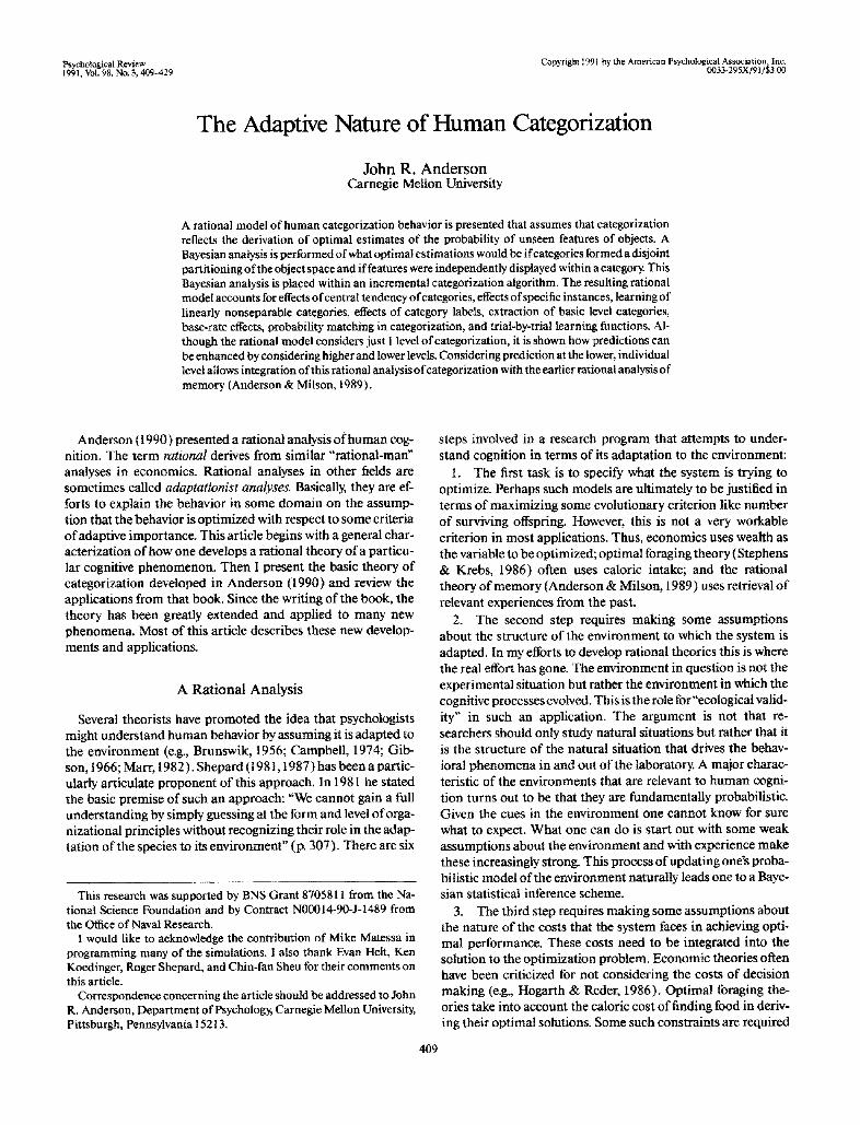
The first experiment in Medin and Schaffer (1978) is a nice one for illustrating the detailed calculations of the algorithm. They had subjects study the following six instances each with binary features:
1 1 1 1 1 1 0 1 0 1 0 1 0 1 1 0 0 0 0 0 0 1 0 0 O 1 0 1 1 0 .
The first four binary values were choices on visual dimensions of size, shape, color, and number. The fifth dimension reflected the category label. They then presented these six objects with- out their category label plus six new objects without a label: 0111-- , 1101--, 1110--, 1000--, 0010--, and 0001--. Sub- jects were to predict the missing category label.
The experiment was simulated by running the program across various random orderings of the stimuli and averaging the results. Figure 1 shows one simulation run where the order was 11111, 10101, 10110, 00000, 01011, and 01000; the cou- pling probability c was .5 (see Equations 4 and 5); and all ai were I (see Equation 10). What is illustrated in Figure 1 is the search behavior of the algorithm as it considers various possible partitionings. The numbers associated with each partition are measures of how probable the new item is, given the category to which it is assigned in that partition. These are the values P(k)P(FIk) calculated by Equations 4-11. Thus, the algo- rithm starts out with categorizing 11111 in the only possible way, that is, assigning it to its own category. The probability of this is the prior probability o fa 1 on each dimension, or (.5)~ = .0313. Then, the two ways to expand this to include 10101, are considered, and the categorization that has both objects in the same category is chosen because that is more likely Each new object is incorporated by considering the possible extensions of the best partition so far. The final choice is the partition (11111,
10101,10110), (00000, 0 I000), (01011 ), which has three cate- gories. Note the system's categorization does not respect the categorization of Medin and Schaffer (1978 ).
Having come up with a particular categorization, the model was tested by presenting it with the 12 test stimuli and assessing the probabilities it would assign to the two possible values for the fifth dimension, which is label. Figure 2 relates the behavior of the algorithm to their data. Plotted along the abscissa are the 12 test stimuli of Medin and Schaffer (1978) in their rank order determined by subjects' confidence that the category label was a 1. The ordinate is the algorithm's probability that the missing value was a 1. Figure 2 illustrates three functions for different ranges of the coupling probability The best rank order correla- tion was obtained for coupling probabilities in the range of .3 and below. At these values the algorithm creates a separate cate- gory for each stimulus, which is what, in effect, the Medin and Schaffer theory claims. However, as shown later, the algorithm does not create singleton categories for all types ofexperimen- tai material at c = .3.
Using a coupling probability of.3 the rank order correlation was .87. Using a coupling probability of.3, rank order correla- tions of.98 and .78 were obtained for two slightly larger experi- mental sets used by Medin and Schaffer (1978). These rank order correlations are as good as those obtained by Medin and Schaffer with their many-parameter model. It also does better than the ACT* simulation reported in Anderson, Kline, and Beasley (1979 ). The coupling probability c is set to. 3 through- out the applications in this article.
The reader will note that the actual probabilities of category labels estimated by the model in Figure 2 only deviate weakly above and below .5. This reflects the very poor category struc- ture of these objects. With better structured material, much higher prediction probabilities are obtained.
Survey o f the Exper imenta l Literature
Anderson (1990) provided a survey of the application of the model to discrete dimensions. This article briefly reviews the results and discusses in more detail some applications that in- volve continuous dimensions.
Central Tendencies
The strongest phenomenon in the literature on human cate- gorization is that the reliability with which an instance is classi- fied decreases as a function of its distance from the central tendency of the category. This trend is so well established now that it is largely ignored in current research, which focuses on the second-order effects. It should be clear that this analysis does predict this main effect. The probability of an item com- ing from a category is a function of its feature similarity (see Equations 6, 10, and 11 ). Anderson (1990) described several cases involving discrete dimensions; this article describes its application to one of the original experiments of prototype for- mation, that of Reed (1972).
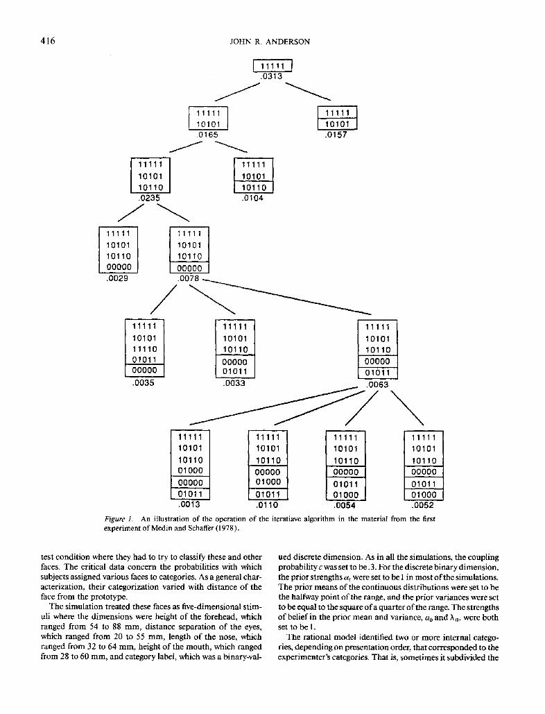
Reed (1972) had subjects learn to categorize the 10 faces that are illustrated in Figure 3. The first row of faces are in one category and the second row of faces are in another category. The two sets of faces are derivations from the prototypes illus- trated in Figure 4. After studying these faces subjects went to a
416 JOHN R. ANDERSON
I 11111 I
J L l1111
10101 .0165
J 11111 I 10101 10110 .0235
11111 i1111 10101 10101 10110 10110 00000 00000 .0029 .0078-.-...
11111
10101 10110 .0104
.0313
11111 10101 .0157
11111 10101 11110 01011 00000
.0035
11111 10101 10110
00000 01011
.0033
11111
10101 10110 00000 01011 .0063
11111 10101 10110 01000
00000 01011 .0013
11111 10101
10110 00000 01000
01011 .0110
11111 10101
10110 00000
01011 O1OO0 .0054
11111 10101 10110 00000
01011 01000 .0052
An illustration of the operation of the iteratiave algorithm in the material from the first Figure 1. experiment of Medin and Schaffer (1978 ).
test condition where they had to try to classify these and other faces. The critical data concern the probabilities with which subjects assigned various faces to categories. As a general char- acterization, their categorization varied with distance of the face from the prototype.
The simulation treated these faces as five-dimensional stim- uli where the dimensions were height of the forehead, which ranged from 54 to 88 ram, distance separation of the eyes, which ranged from 20 to 55 mm, length of the nose, which ranged from 32 to 64 mm, height of the mouth, which ranged from 28 to 60 ram, and category label, which was a binary-val-
ued discrete dimension. As in all the simulations, the coupling probability c was set to be .3. For the discrete binary dimension, the prior strengths a~ were set to be I in most of the simulations. The prior means of the continuous distributions were set to be the halfway point of the range, and the prior variances were set to be equal to the square of a quarter of the range. The strengths of belief in the prior mean and variance, a0 and X o, were both set to be 1.
The rational model identified two or more internal catego- ries, depending on presentation order, that corresponded to the experimenter's categories. That is, sometimes it subdivided the

HUMAN CATEGORIZATION 417
.60
T -
.55
I0
2 . s o
E .45
I,U
• 40 -
I I I 1 I I I I I I I I 1 0 1 1 0 0 1 1 0 1 0 0 1 1 0 1 1 0 1 0 0 0 1 0 1 0 1 0 1 0 1 0 1 1 0 0 1 1 0 1 1 1 0 0 0 1 0 0
c = . 7 - . 8 r = .43
c .2 .3 r .87
c .4 .5 r .66
Figure 2. Estimated probabili~ ~ ofCmegory I for the 12 test stimuli in the first experiment of Medin and Schaffer (1978). (Different functions are for different ranges of the coupling probabiliLv.)
experimenter's categories into subcategories, but it almost never merged items from the two experimenter categories into an internal category Reeds subjects were asked to classify 25 test stimuli, and the major test of the model was its classifica- tion of these test stimuli. Overall its confidence of category membership (calculated by Equation 2) correlated .90 with Reeds data.6
Effects o jSpeci j ic Instances
Although experiments like those of Reed show that human categorization is sensitive to central tendencies, there also has
Fig ure 3. The stimuli used by Reed (I 972 ). (The faces in the first row are in one category and the faces in the second row are in another category. From "Pattern Recognition and Categorization" by S. K Reed, 1972, Cognitive Psychology 3, p. 384. Copyright 1972 by Aca- demic Press. Adapted by permission.)
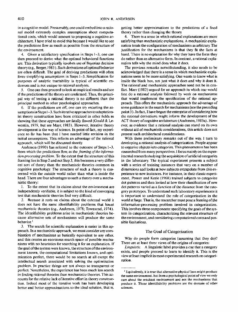
been a great deal of research showing that subjects are sensitive to specific instances that they have studied. Anderson (1990) described simulations of the Medin and Schaffer (1978) experi- ments that demonstrated this effect for discrete dimensions. Here I would like to describe some sinmlations of research by Nosofsky. Figure 5 illustrates the material used by Nosofsky (1988). Subjects were trained to classify 12 colors that varied in brightness and saturation. The colors varied in brightness on the Munsell scale from 3 to 7 and in saturation from 4 to 12. Again in the model of this task, the prior means were set to be the means ofthe dimensions and the prior variances were set to be the squares of one quarter of the ranges. The values for the other parameters were a, = 1, ao = 1, and ~,0 = 1.
In the base condition (B)subjects had four trials on each item and were then tested, in the first experiment there was a Condi- tion E2 in which subjects saw Stimulus 2 approximately 5 times as frequently and a Condition E7 in which they saw Stimulus 7 approximately 5 times as frequently The top panel of Figure 6 illustrates probability of classification in Category 2. As can be seen, subjects are sensitive to the frequency manipulation. The bottom panel of Figure 6 shows the probability that the model assigned to a Category 2 response given the same experience. In Experiment 2, Nosofsky manipulated the frequency of Stimu- lus 6 to be either 3 or 5 times the average (Conditions E6 [ 3 ] and E6 [5 ] ). Figure 7 shows the result and the simulation. In both cases there is sensitivity to the manipulation of the frequency' of Stimulus 6. The overall correlation between data and theory across the two experiments is .98.
Nosofsky took these data as indicating that subjects made
61 thank Stephen Reed for making his data available.
418 JOHN R. ANDERSON
Figure 4. The prototypes for the two categories in Figure 3. (From "Pattern Recognition and Categorization" by S. K. Reed, t972, Cogni- tivePsychology. 3, p. 39 I. Copyright 1972 by Academic Press+ Adapled by permission.)
their judgments o fcategory membership on the basis of similar- ity to individual instances. It is interesting to inquire as to what the rational model was doing. It typically extracted two, three, or four major categories depending on order. For instance, in one run it extracted a category for Stimuli 2, 3, 4, 6, 7, and 9, a category for I and 5, and another category for 8, 10, 11, and 12. In another run it extracted a category for 1, 2, 3, and 5, a cate- gory for 6, a category for 4, 7, and 9, and a category for 8, 10,11, and ) 2. Its category extraction behaviors did not vary as a func- tion of condition. The effect of condition was to bias the center of one of the categories toward the value of the repeated stimu- lus. This would enhance classification of that stimulus.
Linearly Nonseparable Categories
The experiment o fNosofsky (1988) just reviewed is an exam- ple o f an experiment using linearly separable categories, in that
03
W Z
I
ol
| I I I @ I - -1
A ® (9
A ® ®
A ®
A
, , , . A . A , _ _ i
S A T U R A T I O N
Figvre 5. A representation of the material used by Nosofsky 0988). (The circles represent members of one's own category. The triangles represent members of the other category: From "Similarity, Frequency, and Category Representations," by R. M. Nosofsky, 1988, Journal of Experimental Psychology: Learning, Memory, and Cognition. 14, p. 56. Copyright 1988 by the American Psychological Association. Re- printed by permission from the author.)
1.0
• - 0.8 ,,Q t~ .Q o 0.6
0.4 > ,
~ o.2 0
0.0
O b s e r v e d D a t a
E7
. . . . . . . . . . ~. .[}11.~.
1 2 3 4 5 6 7 8 9 10 11 12
c o l o r
P r e d i c t e d D a t a 1 . o -
.-- 0 . 8 - [ ] B pred
E2 pred 0.6 - E7 pred
o 0 . 4 -
~ 0.2
O0 1 2 3 4 5 6 7 8 9 10 11 12
COlOr
Figure 6. Simulation of the first experiment of Nosofsky (1988). (Top: The portion of assignments by subjects of the 12 stimuli to Cate- gory 2 in each of the three conditions. Bottom: The estimated probabil- ity of Category 2 responses by the rational model, B = base condition; E2 = presentation of stimulus 2 approximately 5 times as frequently; E7 = presentation of stimulus 7 approximately 5 times as frequently.)
it is possible to draw a line that separates the two categories. Categories that are linearly separable are easier to learn than categories that are not linearly separable for many categoriza- tion models. However, Medin and Schwanenffugel (1981) showed that subjects can in some circumstances learn linearly nonseparabIe categories more easily than separable categories. This occurs when the instances in the separable categories are all far apart from one another, whereas clusters of within-cate- gory stimuli are close together in the case o f the nonseparable categories. The model reproduces this result because it forms separate internal categories for every cluster of the stimuli. In the case of widely spaced separable stimuli this means a sepa- rate category for every stimulus. In the case o f the nonseparable categories with clusters this means one category for each dus- ter. Thus, there are fewer internal categories to learn in the case of nonseparable external categories.
Table I illustrates the material used by Medin and Schwanen- flugel (1981). In the case of the linearly separable categories it formed separate categories for each stimulus. In the case of linearly nonseparable categories, it merged the first two in Care-

HUMAN CATEGORIZATION 419
Table 1 Abstract Representation of the Alternative Categorization Tasks Used in Experiment 2
Dimension
Exem#ar DI D2 D3 D 4
Linearly separable categories
Category A At 1 1 1 0 A 2 1 0 1 1 A3 1 1 0 1 A4 0 1 1 1
Category B Bl 1 0 1 0 B 2 0 1 1 0 B3 0 0 0 1 B4 1 1 0 0
Categories not linearly separable Category A
Aj 1 0 0 0 A 2 1 0 1 0 A 3 1 1 1 1 A4 0 1 1 1
Category B Bi 0 0 0 1 B2 0 1 0 0 B 3 1 0 1 1 B4 0 0 0 0
Note. Each task involved eight stimuli varying along four dimensions.
Figure 7. Simulation of the second experiment by Nosofsky (1988). (Top: The portion of assignments by subjects of the 12 stimuli to Cate- gory 2 in each of the three conditions. Bottom: The estimated probabil- ity of Category 2 responses by the rational model. B = base condition; E6(3) = Stimulus 6 presented 3 times the average; E6(5) = Stimulus 6 presented 5 times the average.)
gory A into an internal category, the second two in Category A, and the first, second, and fourth in Category B. Thus, only Stimulus 3 in Category B was in a singleton category, and this was the st imulus that produced the highest error rate in their experiment.
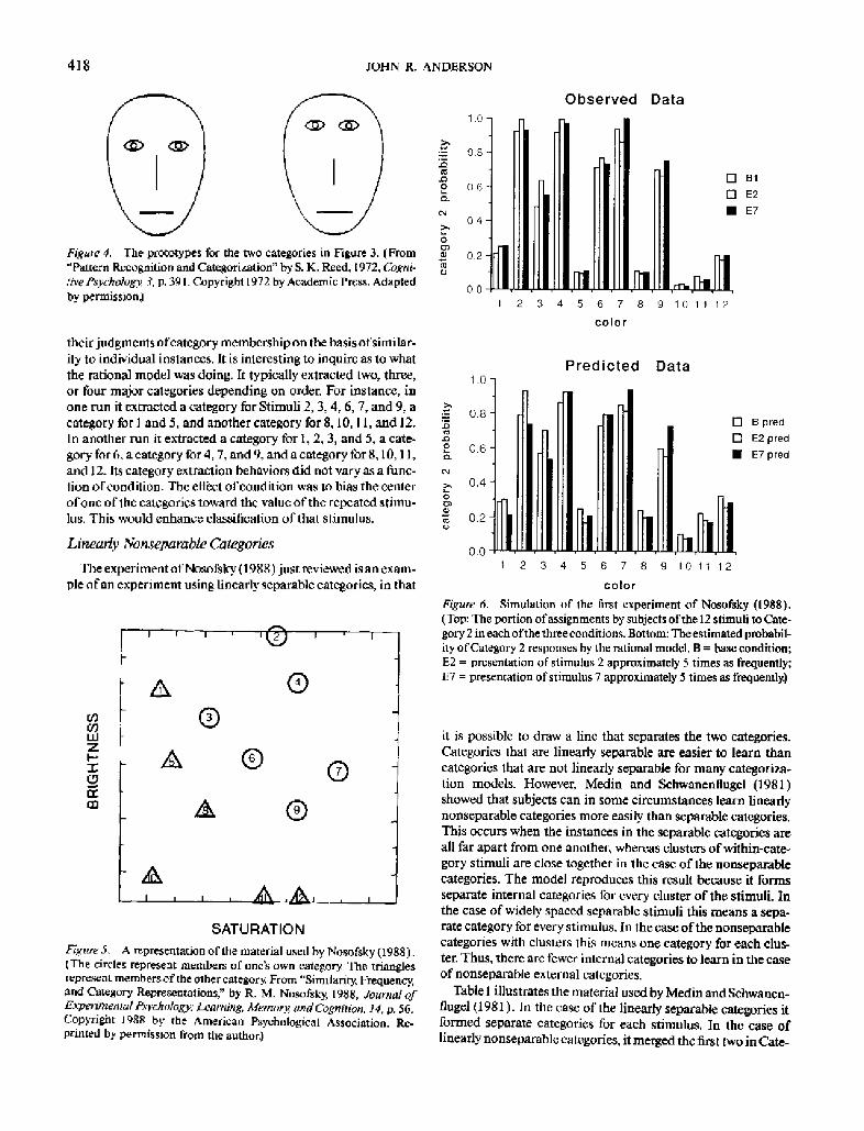
Medin's demonstrat ion was with discrete stimuli. Recently, Nosofsky, et al. (1989) reported a study with cont inuous stim- uli. They had subjects learn to categorize seven circles which varied in size and angle of orientation of a radial line. The four possible sizes were 4.94, 6.17, 8.81, and 10.05 mm, and the four possible angles were 25O, 50 °, 130 °, and 155 °. Figure 8 illustrates the 16 stimuli that resulted from combining these two d imen- sions. Stimuli 1 or 2 were studied and assigned to Category 1 or 2. Subjects were given 150 training trials on these st imuli and then were transferred to a condi t ion where they had to catego- rize all 16 stimuli. Note there is no line that will separate Cate- gory 1 stimuli from Category 2 stimuli.
In typical runs of the model, the simulation extracted four categories, one to contain 1 and 13, one to contain 6 and 10, one to contain 3 and 8, and one to contain 11. In fitting his model to
these data, Nosofsky (1988) had to allow for different atten- t ional sensitivity to the two dimensions of size and angle of rotation and found that the data could be better fit by greater sensitivity to angle. This was modeled in the current framework by allowing separate estimates ofao for the variances on the two dimensions (see Equation 15). The larger a0, the harder it is for a category to have a tight variance, and the category has less sensitivity to that dimension. There was a single estimate of~,o for both dimensions. The parameter a for category label was held at 1 as before, and the coupling parameter c was held at.3 as before. The Stepit program of Chandler (1965 ) was used to find the best fitting values (correlation is.98) of the three free param- eters. The best fitting parameter values were ~o = 31.08, a0 = 2.74 for angle, and a0 = 9.13 for size. Thus, as postulated, the differential sensitivity to dimensions was reproduced by differ- ent prior strengths of the variances. Basically, the model has a stronger belief that a wide range of distances will be equivalent than its belief that a wide range of angles will be equivalent.
Category Labels
The models for the experiments in the last subsection typi- cally extracted more categories than the number of category labels the experimenters use. In the extreme we can induce a separate category for each instance, in which case the model becomes basically indistinguishable from instance-based mod- els (e.g., Medin & Schaffer, 1978; Nosofsky, 1988). It is also possible for the model to merge instances with different cate- gory labels into the same internal category. The likelihood of

420 JOHN R. ANDERSON
A 14 15 16
® ® 12
5 @
A , A
A
1 5.5 12.5 17
ANGLE
Figure 8. The 16 stimuli used by Nosofsky, Clark, and Shin (1989). (The circles were stimuli trained as in Category I and the triangles were stimuli trained as in Category 2. From "Rules andF.~emplars in Cate- gorization, Identification, and Recognition" by R. M.~osofsky, S. E. Clark, and H. J. Shin, 1989, JournalofExperimentalPsych~logy: Learn- ing, Memory, and Cognition, 15, p. 285. Copyright 1989 b~( the Ameri- can Psychological Association. Panel A adapted by p es~ission from the authors.) ' "
j r
this is controlled by a o level for the label dimension; a 0 is the measure of the strength of beliefs in the priors. If this has a low value, there will be a strong bias against merging instances with different category values. Thus, there can be differential sensi- tivity to a dimension like category label. A person is less sensi- tive to empirical data for dimensions about which the person has stronger priors.
It is reasonable that one should have weak priors about a category label. There is no reason to expect that a novel creature encountered in Australia will be called an echidna. It just is. Thus, the general expectation is that internal categories will be at least as refined as the experimenter's category labels. Often they will be more refined, however. It is possible that the setting o fa = l for the category labels in.previous experiments was too high. However, the impact of lowering a would be to decrease the tendency to merge stimuli with different labels. As not much merging occurred with a = l, lowering a would not have substantially changed the behavior.
It is also the capacity to form multiple categories per label that allowed us to fit the data of Medin, Altom, Edelson, and Freko (1982) on correlated features (described in more detail in Anderson, 1990). The problem of characterizing a correlated category structure is very much like solving an exclusive-or problem. The category is defined not by single combination of values on the dimensions but by the fact that when an instance takes a particular value on one dimension it takes a particular value on another dimension. The way the model handles this is to break out a separate internal category for each combination of values. It does this because this maximizes the predictive structure of the instances.
Role of Category Label Feedback
The experiment by Homa and Cultice (1984) is an interesting one for illustrating the role of feedback as to category labels. Figure 9 illustrates their stimulus material. They are derived from the random nine-dot patterns introduced by Posner and Keele (1968), but Homa introduced the feature of drawing lines to connect the dots. This makes it relatively cheap to write a computer program that will determine how to map the points of one into another in a way as to achieve maximal fit. Given such a mapping, one can describe each stimulus according to 18 ordered dimensions, which are the x and y coordinates of each point. The rational categorization model was applied to these materials under such descriptions.
There are three categories in Figure 9 - -one category repre- sented by nine items, one by six, and one by three. In one condi- tion of their experiment, subjects were given category labels and trained to sort the stimuli into three categories. In another condition they were free to sort the stimuli into whatever catego- ries they wanted. Homa and Cultice (1984) were interested in determining how well subjects did at recovering the category structure without feedback. In the case of feedback, Homa and Cultice just measured accuracy of assignment in a final crite- rion test. In the case of no feedback, they tried to discover some way of assigning labels to the categories in the subjects' sort that made their categorization look optimal. It is hard to know how comparable the two measures are.
In the simulation, when there was feedback, the probability of a category label was measured according to Equation 2. When there was no feedback, labels were assigned to internal
Figure 9. (1984).
I I
Examples of low-distortion stimuli from Homa and Cultice

HUMAN CATEGORIZATION 421
- i
*a 0 .60
0 .50
"e 0.40 O = 0.30 (.) "o 0.20 e -
¢= 0.10 ¢= E 0.00 O "I-
(a)
.60 ~ ~ c k
.21
.40 ~edback .04 i |
LOW HIGH Distortion
0.60
= 0 .50 e ) M
0.40
" 0.30 0
m
== 0.20 D _E o.1o (/}
0.00
(b)
Feedback ---<. i ~ b a c k
LOW HIGH Distortion
FigurelO. The results from Homa and Cultice (1984) and the simulation: Performance when the training set is low or high distortion and when there is label feedback or not.
categories in such a way as to maximize probability of a correct label assignment when Equation 2 was used. Again, it is unclear how comparable the two measures were. The measures from the simulation were corrected for guessing. A control condition was run where, rather than letting the algorithm decide which items go together, items were randomly assigned to internal categories. Then performance scores were obtained in the same way as when the algorithm did the assignment. Thus, there were two measures--P, a mean probability of the correct category label when the algorithm did the clustering and G, a mean probability of category labeling in the control condition when the clustering was done randomly The final measure was ( P - G)/(1 - G), which is a standard correction-for-guessing for- mula.
Homa and Cultice (1984) used several different training sets, including a low distortion training set where the points were perturbated 1.1 units (the examples in Figure 9 are 1.1 distor- tions) and a high distortion set where they were perturbated 4.8 units. Figure 10 compares the performance of the subjects and the simulation for high- and low-distortion training stimuli in the presence of label feedback or not. In the case of Homa and Cultice, a correction for guessing measure was used with G set to be .33, because there were three categories. Both subjects and simulations show approximately additive effects of the two di- mensions. Both the subjects and the simulation are nearly at chance in the presence of high distortion stimuli with no label feedback. However, the model shows greater sensitivity to feed- back.
In summary, subjects and the model appear capable of iden- tifying category structure in the absence of feedback when there is a relatively obvious category structure. When such an obvious structure is missing, the category label provides a neces- sary cue. Even when there is a relatively obvious category struc- ture, a category label provides yet an additional correlated cue and so enhances categorization.
Learning Trends
The results to this point have been concerned with compar- ing the final performance of the algorithm with the final perfor- mance of humans. However, recently there has been growing interest in comparing the course of learning in categorization.
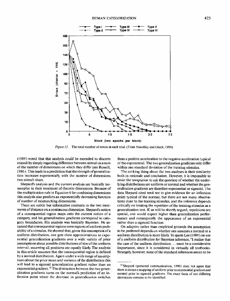
Some of the most intricate data on this score are unpublished data by Nosofsky and Gluck (1989 ), who did a further analysis of learning with the stimuli ofShepard, Hovland, and Jenkins, (1961 ) illustrated in Figure 11. They looked at the task of trying to categorize eight stimuli defined by binary values on three dimensions into two categories of four items. Figure 11 illus- trates the six logically possible ways of dividing these catego- ries. Shepard et al. found that Category I was easiest to learn; followed by II; followed by III, IV, and V, which were essentially equivalent; followed by VI. Figure 12 shows the learning data recently obtained by Nosofsky and Gluck for 25 trials. 7 The superiority of Class II emerges relatively late in the categoriza- tion, but otherwise the results of Shepard et al. are confirmed. Kruschke (1990) noted that the ease of the Class II structure relative to the more prototypical structures like IV is problemat- ical for a good many category models (although his ALCOVE model with attentional parameters is able to handle these re- sults). Basically, Type II involves two distant clusters within a category The categories in Type II are not linearly separable. On the other hand, the stimuli can be categorized by only pay- ing attention to two dimensions.
Figure 13 displays the learning results of the application of the model with the parameters cq = .01 for the category label and 1.0 for all other dimensions. As can be seen the model does a good job of replicating the learning trends including the late emergence of the superiority of Type II? It will also be noted that the model produces an interesting pattern with Type IV where it starts out as one of the best but shows a residual diffi- culty so that it becomes as bad as Type VI. This pattern also appears in the data.
Each trial was modeled as another presentation of the eight
7 Each subject was in all six conditions, but Nosofsky and Gluck (1989 ) presented the results from the last three conditions a particular subject was in. Error rate was higher in the first three than the last three.
8 Figure 13 plots estimated probability of the incorrect category la- bel. These probabilities remain above zero even after 25 exposures to each stimulus, in contrast to Figure 12 where most conditions go down to zero error rate. However, it is not unreasonable to suppose that once estimated probability gets to something like 90% for a category label, subjects will always assign that label, thereby producing zero error rate.
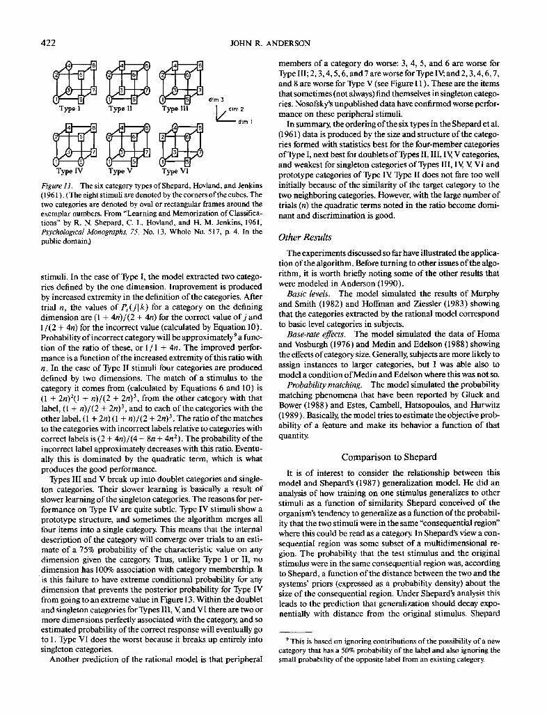
422 JOHN R. ANDERSON
Type I Type I! Type III ~/dim 2
d~m I
Type IV Type V Type Vl
Figure 11. The six category types ofShepard, Hovland, and Jenkins (1961 ). ( The eight stimuli are denoted by the corners of the cubes. The two categories are denoted by oval or rectangular frames around the exemplar numbers. From "Learning and Memorization of Classifica- tions" by R. N. Shepard, C. L. Hovland, and H. M. Jenkins, 1961, Psychological Monographs, 75, No. 13, Whole No. 517, 13. 4. In the public domain.)
stimuli. In the case of Type I, the model extracted two catego- ries defined by the one dimension. Improvement is produced by increased extremity in the definition of the categories. After trial n, the values of Pi (Jl k) for a category on the defining dimension are (1 + 4n)/(2 + 4n) for the correct value o f j and l / ( 2 + 4n) for the incorrect value (calculated by Equation 10). Probability of incorrect category will be approximately 9 a func- tion of the ratio of these, or 1 / 1 + 4n. The improved perfor- mance is a function of the increased extremity of this ratio with n. In the case of Type II stimuli four categories are produced defined by two dimensions. The match of a stimulus to the category it comes from (calculated by Equations 6 and 10) is (1 + 2n)2(1 + n)/(2 + 2n) 3, from the other category with that label, (1 + n)/(2 + 2n) 3, and to each of the categories with the other label, (1 + 2n) (1 + n)/(2 + 2n) 3. The ratio of the matches to the categories with incorrect labels relative to categories with correct labels is (2 + 4n)/(4 + 8n + 4n2). The probability of the incorrect label approximately decreases with this ratio. Eventu- ally this is dominated by the quadratic term, which is what produces the good performance.
Types III and V break up into doublet categories and single- ton categories. Their slower learning is basically a result of slower learning of the singleton categories. The reasons for per- formance on Type IV are quite subtle. Type IV stimuli show a prototype structure, and sometimes the algorithm merges all four items into a single category. This means that the internal description of the category will converge over trials to an esti- mate of a 75% probability of the characteristic value on any dimension given the category Thus, unlike Type I or II, no dimension has 100% association with category membership. It
i s this failure to have extreme conditional probability for any dimension that prevents the posterior probability for Type IV from going to an extreme value in Figure 13. Within the doublet and singleton categories for Types III, V, and VI there are two or more dimensions perfectly associated with the category, and so estimated probability of the correct response will eventually go to 1. Type VI does the worst because it breaks up entirely into singleton categories.
Another prediction of the rational model is that peripheral
members of a category do worse: 3, 4, 5, and 6 are worse for Type III; 2, 3, 4, 5, 6, and 7 are worse for Type I ~ and 2, 3, 4, 6, 7, and 8 are worse for Type V (see Figure 11 ). These are the items that sometimes (not always) find themselves in singleton catego- ries. Nosofsky's unpublished data have confirmed worse perfor- mance on these peripheral stimuli.
In summary, the ordering of the six types in the Shepard et al. (1961) data is produced by the size and structure of the catego- ries formed with statistics best for the four-member categories of Type I, next best for doublets of Types II, III, IV, V categories, and weakest for singleton categories of Types III, IV, V, VI and prototype categories of Type IV. Type II does not fare too well initially because of the similarity of the target category to the two neighboring categories. However, with the large number of trials (n) the quadratic terms noted in the ratio become domi- nant and discrimination is good.
Other Results
The experiments discussed so far have illustrated the applica- tion of the algorithm. Before turning to other issues of the algo- rithm, it is worth briefly noting some of the other results that were modeled in Anderson (1990).
Basic levels. The model simulated the results of Murphy and Smith (1982) and Hoffman and Ziessler (1983) showing that the categories extracted by the rational model correspond to basic level categories in subjects.
Base-rate effects. The model simulated the data of Homa and Vosburgh (1976) and Medin and Edelson (1988) showing the effects of category size. Generally, subjects are more likely to assign instances to larger categories, but I was able also to model a condition of Medin and Edelson where this was not so.
Probability matching. The model simulated the probability matching phenomena that have been reported by Gluck and Bower (1988) and Estes, Cambell, Hatsopoulos, and Hurwitz (1989 ). Basically, the model tries to estimate the objective prob- ability of a feature and make its behavior a function of that quantity
C o m p a r i s o n to S h e p a r d
It is of interest to consider the relationship between this model and Shepard's (1987) generalization model. He did an analysis of how training on one stimulus generalizes to other stimuli as a function of similarity Shepard conceived of the organism's tendency to generalize as a function of the probabil- ity that the two stimuli were in the same "consequential region" where this could be read as a category. In Shepard's view a con- sequential region was some subset of a multidimensional re- gion. The probability that the test stimulus and the original stimulus were in the same consequential region was, according to Shepard, a function of the distance between the two and the systems' priors (expressed as a probability density) about the size of the consequential region. Under Shepard's analysis this leads to the prediction that generalization should decay expo- nentially with distance from the original stimulus. Shepard
9 This is based on ignoring contributions of the possibility of a new category that has a 50% probability of the label and also ignoring the small probability of the opposite label from an existing category.
180"
162"
144
126"
II
~ 108" o C
o 90"
P 8 72- L.
54'
36"
18"
O+ 0
Figure 12.
HUMAN CATEGORIZATION
A Type I • Type III : Type V Type II o----- Type IV ----m---- Type VI
5 1 0 1 5 2 0 2 5
Block ( two e p o c h s per b lock)
The total number of errors in each trial. (From Nosofsky and Gluck, 1989.)
423
(1989) noted that this analysis could be extended to discrete stimuli by simply regarding difference between stimuli as a sum of the number of dimensions on which they differ (see Russell, 1986). This leads to a prediction that the strength of generaliza- tion increases exponentially with the number of dimensions two stimuli share.
Shepard's analysis and the current analysis are basically iso- morphic in their treatment of discrete dimensions. Because of the multiplication rule in Equation 6 for combining dimensions this analysis also predicts an exponentially decreasing function of number of mismatching dimensions.
There are subtle but informative contrasts in the two treat- ments of distance on a continuous dimension. Shepard's notion of a consequential region maps onto the current notion of a category, and his generalization gradients correspond to cate- gory boundaries. His analysis was basically Bayesian. He as- sumed that consequential regions were regions of uniform prob- ability of a stimulus. He showed that, given this assumption of a uniform distribution, one gets close approximations to expo- nential generalization gradients over a wide variety of prior assumptions about possible distributions of size of the uniform interval, assuming all positions are equally likely. The analysis in this article assumes that the consequential region is defined by a normal distribution. Again under a wide range of assump- tions about the prior mean and variance of the distribution this will lead to a sigmoid generalization gradient rather than an exponential gradient.I° The distinction between the two gener- alization gradients turns on the normal's prediction of an in- flection point where the decrease in generalization switches
from a positive acceleration to the negative acceleration typical of the exponential. The two generalization gradients only differ within one standard deviation of the training stimulus.
The striking thing about the two analyses is their similarity both in rationale and conclusion. However, it is impossible to resist the temptation to ask the question of whether the under- lying distributions are uniform or normal and whether the gen- eralization gradients are therefore exponential or sigmoid. The data Shepard cited tend not to give evidence for an inflection point typical of the normal, but there are not many observa- tions close to the training stimulus, and the inference depends critically on treating the repetition of the training stimulus as a generalization test. If, as will be shortly argued, repetitions are special, one would expect higher than generalization perfor- mance and consequently the appearance of an exponential rather than a sigmoid function.
On adaptive rather than empirical grounds the assumption to be preferred depends on whether one assumes a normal or a uniform distribution is more likely. To quote Lee (1989) on use of a uniform distribution for Bayesian inference, "I realize that the case of the uniform dis t r ibut ion . . , must be a considerable importance, since it is considered in virtually all textbooks. Strangely, however, none of the standard references seems to be
~0 Shepard (personal communication, 1990) does not agree that there is always a mapping of uniform prior to exponential gradient and normal prior to sigmoid gradients. The exact basis of our differing derivations remains to be identified.
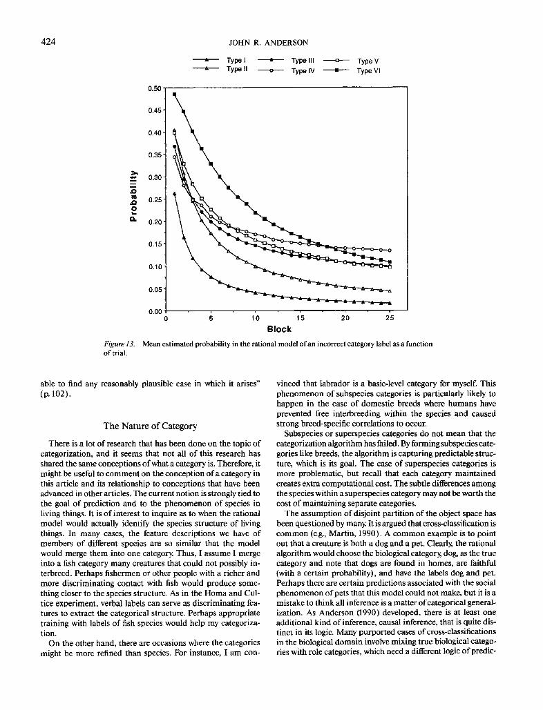
424 JOHN R. ANDERSON
. D
B
° n e ~
e ~
o i .
o.
A Typel • Typell l ~ TypeV A Type II ~ Type IV • Type Vl
Figure 13. of trial.
0.50"
0.45'
0.40
0.35
0.30
0.25
0.20
0.15
0.10
0.05
0.00 0 5 1 '0 1 '5 2'0 2'5
B l o c k
Mean estimated probabil i ty in the rational model o f an incorrect category label as a function
able to find any reasonably plausible case in which it arises" (p. 102).
The Na tu re o f Ca tegory
There is a lot of research that has been done on the topic of categorization, and it seems that not all of this research has shared the same conceptions of what a category is. Therefore, it might be useful to comment on the conception of a category in this article and its relationship to conceptions that have been advanced in other articles. The current notion is strongly tied to the goal of prediction and to the phenomenon of species in living things. It is of interest to inquire as to when the rational model would actually identify the species structure of living things. In many cases, the feature descriptions we have of members of different species are so similar that the model would merge them into one category. Thus, I assume I merge into a fish category many creatures that could not possibly in- terbreed. Perhaps fishermen or other people with a richer and more discriminating contact with fish would produce some- thing closer to the species structure. As in the Homa and Cul- tice experiment, verbal labels can serve as discriminating fea- tures to extract the categorical structure. Perhaps appropriate training with labels of fish species would help my categoriza- tion.
On the other hand, there are occasions where the categories might be more refined than species. For instance, I am con-
vinced that labrador is a basic-level category for myself. This phenomenon of subspecies categories is particularly likely to happen in the case of domestic breeds where humans have prevented free interbreeding within the species and caused strong breed-specific correlations to occur.
Subspecies or superspecies categories do not mean that the categorization algorithm has failed. By forming subspecies cate- gories like breeds, the algorithm is capturing predictable struc- ture, which is its goal. The case of superspecies categories is more problematic, but recall that each category maintained creates extra computational cost. The subtle differences among the species within a superspecies category may not be worth the cost of maintaining separate categories.
The assumption of disjoint partition of the object space has been questioned by many. It is argued that cross-classification is common (e.g., Martin, 1990). A common example is to point out that a creature is both a dog and a pet. Clearly, the rational algorithm would choose the biological category, dog, as the true category and note that dogs are found in homes, are faithful (with a certain probability), and have the labels dog and pet. Perhaps there are certain predictions associated with the social phenomenon of pets that this model could not make, but it is a mistake to think all inference is a matter of categorical general- ization. As Anderson (1990) developed, there is at least one additional kind of inference, causal inference, that is quite dis- tinct in its logic. Many purported cases of cross-classifications in the biological domain involve mixing true biological catego- ries with role categories, which need a different logic of predic-
HUMAN CATEGORIZATION 425
tion. Just because language treats both dog and pet as nouns does not mean the mind treats their referents identically.
This confusion of linguistic labeling and categories is at the heart of Barsalou's (1983) point about ad hoc categories. He claimed people can make up categories on the spur of the mo- ment, such as "things to take from a burning house" However, just because one can create an appropriate noun phrase, its referent does not become a mental category. To be sure, we can reason about such ad hoc categories, but such reasoning in- volves causal inference and not categorical inference.
Some people (e.g., Murphy & Medin, 1985) have questioned the extent to which similarity-based categories exist and have argued that most categories are theory based. They point out that people display rich rules for reasoning about objects and can, for instance, overcome visual appearance to infer bats and dolphins are mammals (rather than birds and fish) and hence suckle their young. Most cited cases of such theory-based cate- gories involve levels of aggregation much higher than would be produced by the rational model. For instance, mammal is un- likely to be a category in the model at hand--dolphins and bats are more likely (and both of which are still superspecies catego- ries). One could capture these facts by just storing the mammal label and the suckle-their-young property as features of the bat and dolphin category. However, this would miss the point of such examples, which is that one can infer that a bat suckles it young from the fact that it is a mammal without any direct evidence that bats suckle their young. Such predictions are not captured in this rational model of categorization. However, it is an open question whether the ability to make such predictions reflects anything about natural categories or whether it reflects the application of schoolroom knowledge acquired quite sepa- rately
As noted throughout the article, category labels are treated as just another feature to be predicted that may differ in their prior parameters but that do not differ in their logical role. It is remarkable that very little laboratory research has been done to see if category labels are in fact special. Recently, Heit (1990) looked at the question of whether category labels are different from any other stimulus feature in terms of serving as a cue for prediction or as a feature to be predicted. His result was that category labels are not different.
It should be acknowledged however that there are a strong set of linguistic phenomena associated closely with categories (e.g., Markman, 1989). These linguistic categories are presumably quite functional in communicating information. It is legitimate to try to study and understand these phenomena surrounding these linguistic categories. However, I question what they have to do with the sense of category that is the topic of this article. The categories of this article are potentially nonverbal, non- conscious, and need only be implicit in prediction behavior.
H ie r a r ch i ca l S t ruc tu re
Another peculiar feature of this model is that it identifies a particular distinguished level that is the basic level. Language, on the other hand, allows for a hierarchy of categorical expres- sions. A natural question is whether there is any role for such a hierarchy of categories in the rational model. In fact, one could achieve some greater predictive accuracy by considering levels of aggregation above and below the category. I consider what
could be gained by having a level of aggregation above the cate- gory, called the genus 1~ level, and a level below, which is the individual level (corresponding to different appearances of the same object).
Genus-Level Identification
The genus level offers a level of aggregation above the species. A genus corresponds to a group of biologically related species that are more similar to one another than are arbitrary pairs of species. The significance of the genus level does not come in making predictions about known properties of known species. For instance, we are much better off predicting the cat-chasing propensity of Fido knowing that he is a dog than knowing he is a mammal. The significance of the genus level comes in mak- ing predictions about unknown properties of a known species (e.g., whether Fido has a spleen) and making predictions about unknown species.
In Bayesian terms, the significance of the genus level is that it can be used to set more informed priors for the species under the genus. This will help in making predictions about new spe- cies and about unexperienced properties of existing species. The interesting complication is that these priors themselves depend on estimates of the parameters for the existing species, which in turn depend on the priors. Thus, it might seem that there is a difficult joint estimation problem. The typical Baye- sian approaches to such estimation problems are called hierar- chical methods (Berger, 1985, Section 4.6). The technical devel- opment of such methods can be quite complex and is not justi- fied here, because data have not yet been gathered that require such complex quantitative analysis. It is enough to note for current purposes that there is a rationale for making estimates of the mean and variance within a species sensitive to estimates of means and variances for other species within a genus.
There certainly is evidence that people have this sensitivity. Even young children have expectations about the properties of new types of animals on the basis of animals that they have seen (Carey, 1985). They also have expectations that certain dimen- sions are less variable for certain types of categories. Thus, there is the expectation that animals within a category will have the same constitution, whereas artifacts within a category will have the same function (Gelman, 1988). Moreover, these ex- pectations show developmental trends to more accurate forms as experience accumulates.
The experiment of Nisbett, Krantz, Jepson, and Kunda (1983 ) also illustrated differential sensitivity to variance in cate- gories of different kinds. They asked subjects to suppose that they had a sample of a new mineral, a new bird, or a new tribe of people from a new island. They were given samples of different sizes and told that all the objects within the sample had some property. Subjects were willing to extrapolate from a single ob- servation for some dimensions, like conductivity of the mineral or skin color of the tribe of people, whereas they required 20
tl My use of the term genus is in its more general sense to refer to a kind and does not imply the precision that is involved in the distinction among genus, family, order, class, and phylum in biology. I suspect that the level useful in prediction might be considerably above the biologi- cal genus level and actually closer to the phylum level.

426 JOHN R. ANDERSON
observations before they were able to extrapolate with any con- fidence for other dimensions, like the obesity of the people.
This ability to show sensitivity to variance is one thing that distinguishes this hierarchical Bayesian approach to categoriza- tion from most others. Many approaches (e.g., instance-based models) would predict that subjects would be biased in their estimate of the mean of a new species by the mean of existing species. These other approaches do not have the mechanisms, however, for showing a similar sensitivity to variance.
Individual-Level Identification
The individual level provides a much lower level of aggrega- tion below the category. For purposes of prediction, there is a real advantage to identifying a repetition of an individual and making predictions from the individual rather than the cate- gory. This is because the individual may reliably deviate from the mean of the category and because many features are much more certain at the individual level than at the category.
Retrieving an individual and making a prediction on this basis corresponds to a memory retrieval. From this perspective the difference between memory and categorization concerns whether prediction is being made at the individual level or the category level. It is basically the same logic of prediction; how- ever, it needs to be parameterized differently. To reflect the fact that individuals repeat themselves much less often than catego- ries, a lower value of the coupling parameter c should be used. Also, the features are much less likely to change, and to accom- modate this fact, there should be lower values of the ai for discrete dimensions and much smaller values of %2 for con- tinuous.
Thus, the identification of the individual is modeled in the same way as identification of a category except that the assump- tion is that individuals repeat themselves less frequently-- hence, the lower c value. This perspective takes the point of view that when people encounter a new instance it is ambigu- ous whether it is a new individual or some old individual just as it is ambiguous whether it is a new category or some old cate- gory The prior probability of an individual and the similarity of the presented instance to the remembered individual are used to decide if the presented instance is an old individual in just the way a category is recognized.
There has been a lot of speculation as to how categorization behavior relates to memory behavior. The instance-based mod- els (Medin & Schaffer, 1978; Nosofsky, 1986) would argue that everything is really instance based, whereas connectionist mod- els (McClelland, Rumelhart, & Hinton, 1986) would argue that there are no separate representations of instances and every- thing is merged together. They try to account for differences between categorization and memory by arguing that a single representation is differently processed. The current rational ap- proach offers a representation that distinguishes the two levels but uses the same Bayesian logic at both levels. Of course, the rational representation is only an acknowledgment of the fact that there are individuals and categories in the real world. It does not really make any claims about how they are processed in the head.
There is one analysis and prediction that does follow from a rational analysis that does not seem to flow from the other models. This concerns the fan effect (Anderson, 1983b). Typi-
caUy it is described in other terms, but in current terminology it is concerned with the effect of repeating a value on a dimension for multiple individuals or items. Memory for specific items is hurt by repeating a feature across multiple items. On the other hand, if the feature is consistently associated with a category, categorization is enhanced when the feature is repeated (Reder & Ross, 1983). The contrast between these two fan effects can be illustrated with respect to the material in Table 2 typical of those used in Reder and Anderson (1980) or Reder and Ross (1983).
Subjects studied a set of target sentences. In terms of the analysis in this article, each sentence is like an item composed of features. Table 2 gives the feature code used for each sentence in the simulation. There are four dimensions: The first corre- sponds to the person; the second to the theme of the predicate; the third to the specific predicate; and the fourth to whether the item was studied. Thus "George bought a train ticket" is en- coded as (2 0 5 0), where 2 refers to George, the first 0 to the train theme, the 5 to the specific predicate, and the 0 to the fact that it was studied. Table 2 also gives the fan of these materials, which is the number of items in which the person occurs.
When subjects are in a memory experiment, they are asked to judge whether specific sentences had been studied. In this case related foils such as those in Table 2 are used. A related foil is created by pairing persons with predicates of the same theme that had been studied with other persons. When subjects are in a categorization experiment, they are asked to judge whether the sentence is like the sentences they had studied. In this case an unrelated foil is created by pairing persons with predicates of different themes.
These two conditions were simulated not just by presenting the different sets of materials that the subject saw to the model but also by adjusting the parameters. In the case of a categoriza- tion task, c was set to .3 as usual, whereas it was set to .03 in the case of a memory task. 12 In both experiments the o/i corre- sponding to the fourth dimension was set very low at .001. This reflects the idea that sentences cannot both be studied and not studied. The setting of the ai for the other dimensions de- pended on the task. In the case of categorization, the usual value of 1.0 was used, whereas in the memory task the more extreme value of 0.1 was used to reflect constancy of features across repetitions of an instance. These differences seemed a priori plausible ways to model the task, but the results depend critically only on the setting of the c parameter.
In the category condition, the model extracts four categories defined by crossing the two sets of thematically related sen- tences crossed with whether they are studied or not. In the memory condition the various true and false sentences are identified as the individuals.
The model was tested by presenting it with stimuli with the last dimension (presentation status) omitted and asking the model to predict the presentation status. The results are shown in Figure 14(right panel) in terms of the models estimation of the probability of a correct response. For the sake of compari- son, the left panel gives the data from Reder and Ross in terms
~2 At this value of c, the system will treat a repetition of an item as the same category. It will not at c = .01. At c = .10, it will not extract the items as categories.

HUMAN CATEGORIZATION
Table 2 Materials Used in Simulation of Positive and Negative Fan Effects
Item Fan Feature code
Target Marly arrived at the train station Marly heard the train conductor Marly took the train to Grand Central Fred checked the train schedule Fred waited for the train George bought a train ticket
Tom preferred to run on the inside lane Tom did sprints to improve speed Tom bought a new pair of Adidas Bill warmed up by jogging Bill ran five miles Mike wanted to make the track team
Related foil Marly checked the train schedule Marly waited for the train Marty bought a train ticket Fred arrived at the train station Fred heard the train conductor George took the train to Grand Central
Tom warmed up by jogging Tom ran five miles Tom wanted to make the track team Bill preferred to run on the inside lane Bill did sprints to improve speed Mike bought a new pair of Adidas
Unrelated foil Marly warmed up by jogging Marry ran five miles Marly wanted to make the track team Fred preferred to run on the inside lane Fred did sprints to improve speed George bought a new pair of Adidas
Tom checked the train schedule Tom waited for the train Tom bought a train ticket
Bill arrived at the train station Bill heard the train conductor Mike took the train to Grand Central
3 (00 00) 3 (00 10) 3 (00 20) 2 (10 30) 2 (10 40) 1 ( 2 0 50 )
3 (31 60) 3 (31 70) 3 (31 80) 2 (41 90) 2 (41100) 1 ( 5 1 1 1 O)
3 (00 31) 3 (00 41) 3 (00 5 0 2 (10 01) 2 (1 o 1 1) 1 (20 21)
3 (31 91) 3 (31101) 3 (31111) 2 (41 61) 2 (41 71) 1 (51 81)
3 (01 91) 3 (0110 l) 3 (0111 l) 2 (11 61) 2 (1 1 7 I) 1 (21 81)
3 (30 31) 3 (30 41) 3 (30 51)
2 (40 01) 2 (40 11) 1 ( 5 0 21)
427
of mean time for a correct response. The correspondence is compelling. In the case of a categorical response, repetition of an item leads to an increased certainty of the response, because this increases the match to the theme category. In the case of a memory response, increased fan means increased match to ir- relevant foils and hence lower certainty of a match to the item. Thus, the interaction with fan and task is a reasonable statisti- cal response to the task structure.
This points the way to a merging of the rational model of memory (Anderson & Milson, 1989) and this rational model of categorization. Anderson and Milson calculated the probabil- ity of a memory trace being needed as a product of prior proba- bility and a conditional probability of a trace given cues. This maps onto Equation 3 in the current analysis. Casting memory in the current categorization framework enables a much more sophisticated analysis of the conditional probabilities. More- over, the point of memory retrieval is better articulated, which is not just to get at a needed trace but to use these traces to make predictions (e.g., where the car is parked). On the other hand,
the memory model had a much more sophisticated analyses of the prior probability, incorporating recency, frequency, and spacing. It also offered a model of how the internal probabilities mapped onto dependent measures like probability correct and reaction time. Although development of a complete integration of the two models remains a future goal, it does appear a promis- ing direction.
Conc lus ion
Although more research remains to be done on this rational model of categorization, a good case has been made for the proposition that categorization behavior can be predicted from the structure of the environment at least as well as it can from the structure of the mind. Most of the studies reviewed in this article already had been fitted to one or more categorization models. The typical observation when the rational model is compared with one of these models is that the two models corre- late better with each other than either do with the data. This
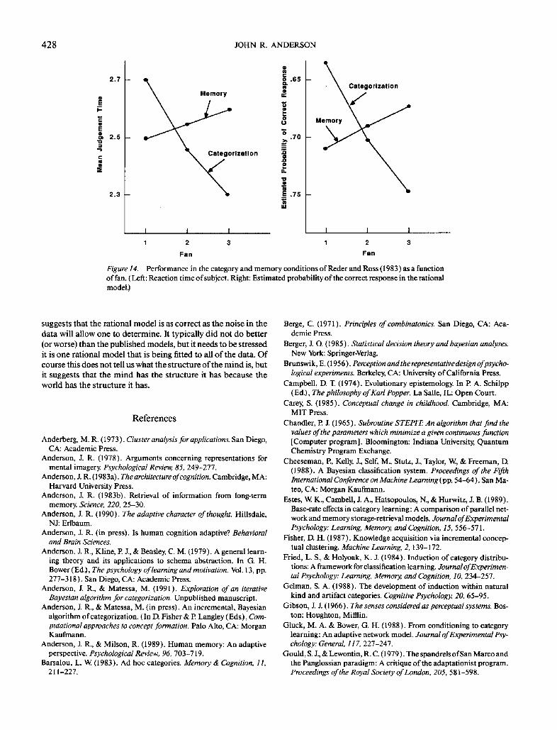
428 JOHN R. ANDERSON
2.7
o E I -
Q 2.5
i - 1o o :E
2.3
.~ .ss
orlzatlon
a .
E.75 IlJ
- M ~ ~tg°rizatl°n
I I I I I I
1 2 3 1 2 3 Fan Fan
Figure 14. Performance in the category and memory conditions of Reder and Ross (1983) as a function of fan. (Left: Reaction time of subject. Right: Estimated probability of the correct response in the rational model.)
suggests that the rational model is as correct as the noise in the data will allow one to determine. It typically did not do better (or worse) than the published models, but it needs to be stressed it is one rational model that is being fitted to all o f the data. Of course this does not tell us what the structure o f the mind is, but it suggests that the mind has the structure it has because the world has the structure it has.
References
Anderberg, M. R. (1973). Cluster analysis for applications. San Diego, CA: Academic Press.
Anderson, J. R. (1978). Arguments concerning representations for mental imagery. Psychological Review, 85, 249-277.
Anderson, J. R. (1983a). The architecture of cognition. Cambridge, MA: Harvard University Press.
Anderson, J. R. (1983b). Retrieval of information from long-term memory. Science, 220, 25-30.
Anderson, J. R. (1990). The adaptive character of thought. Hillsdale, N J: Erlbaum.
Anderson, J. R. (in press). Is human cognition adaptive? Behavioral and Brain Sciences.
Anderson, J. R., Kline, P. J., & Beasley, C. M. (1979). A general learn- ing theory and its applications to schema abstraction. In G. H. Bower (Ed.), The psychology of learning and motivation. Vol. 13, pp. 277-318). San Diego, CA: Academic Press.
Anderson, J. R., & Matessa, M. (1991). Exploration of an iterative Bayesian algorithm for categorization. Unpublished manuscript.
Anderson, J. R., & Matessa, M. (in press). An incremental, Bayesian algorithm of categorization. (In D. Fisher & P. Langley (Eds.), Com- putational approaches to concept formation. Palo Alto, CA: Morgan Kaufmann.
Anderson, J. R., & Milson, R. (1989). Human memory: An adaptive perspective. Psychological Review., 96, 703-719.
Barsalou, L. W. (1983). Ad hoc categories. Memory & Cognition, 11, 211-227.
Berge, C. (1971). Principles ofcombinatonics. San Diego, CA: Aca- demic Press.
Berger, J. O. (1985 ). Statistical decision theory and bayesian analyses. New York: Springer-Verlag.
Brunswik, E. (1956). Perception and the representative design of psycho- logical experiments. Berkeley, CA: University of California Press.
Campbell, D. T. (1974). Evolutionary epistemology. In P. A. Schilpp (Ed.), The philosophy of Karl Popper. La Salle, IL: Open Court.
Carey, S. (1985). Conceptual change in childhood. Cambridge, MA: MIT Press.
Chandler, E J. (1965). Subroutine STEPIT." An algorithm that find the values of the parameters which minimize a given continuous function [Computer program]. Bloomington: Indiana University, Quantum Chemistry Program Exchange.
Cheeseman, P., Kelly, J., Self, M., Stutz, J., Taylor, W., & Freeman, D. (1988). A Bayesian classification system. Proceedings of the Fifth International Conference on Machine Learning ( pp. 54-64). San Ma- teo, CA: Morgan Kaufmann.
Estes, W. K., CambeU, J. A., Hatsopoulos, N., & Hurwitz, J. B. (1989). Base-rate effects in category learning: A comparison of parallel net- work and memory storage-retrieval models. Journal of Experimental Psychology: Learning, Memory, and Cognition, 15, 556-571.
Fisher, D. H. (1987). Knowledge acquisition via incremental concep- tual clustering. Machine Learning, 2, 139-172.
Fried, L. S., & Holyoak, K. J. (1984). Induction of category distribu- tions: A framework for classification learning. JournalofExperimen- tal Psychology: Learning, Memory, and Cognition, 10, 234-257.
Gelman, S. A. (1988). The development of induction within natural kind and artifact categories. Cognitive Psychology, 20, 65-95.
Gibson, J. J. (1966). The senses considered as perceptual systems. Bos- ton: Houghton, Mifflin.
Gluck, M. A. & Bower, G. H. (1988). From conditioning to category learning: An adaptive network model. Journal of Experimental Psy- chology: General 117, 227-247.
Gould, S. J., & Lewontin, R. C. (1979). The spandrels of San Marco and the Panglossian paradigm: A critique of the adaptationist program. Proceedings of the Royal Society of London, 205, 581-598.
HUMAN CATEGORIZATION 429
Heit, E. (1990). Reasoning from examples. Unpublished doctoral dis- sertation, Stanford University.
Hoffman, J., & Ziessler, C. (1983). Objectidentifikation in kunstlichen Bergriffshierarcchien [Object identification ] Zeitschrift fur Psycho- logie, 194, 135-167.
Hogarth, R. M., & Reder, M. W. (1986 ). The behavioral foundations of economic theory. Journal of Business, 59(4, Pt. 2).
Homa, D., & Cultice, J. (1984). Role of feedback, category size, and stimulus distortion in the acquisition and utilization of ill-defined categories. Journal of Experimental Psychology: Learning, Memory, and Cognition, I0, 83-94.
Homa, D., & Vosburgh, R. (1976). Category breadth and abstraction of prototypical information. Journal of Experimental Psychology." Hu- man Learning and Memory, 2, 322-330.
Kruschke, J. K. (1990, June). ALCOVE: A connectionist model of cate- gorylearning(Tech. Rep. No. 19). Cognitive Science, Indiana Univer- sity, Bloomington, IN.
Lebowitz, M. (1987). Experiments with incremental concept forma- tion: UNIMEM. Machine Learning, 2, 103-138.
Lee, E M. (1989). Bayesian statistics. New York: Oxford University Press.
Markman, E. M. (1989 ). Categorization and naming in children: Prob- lems of induction. Cambridge, MA: MIT Press.
Mart, D. (1982). Vision. San Francisco: Freeman. Martin, J. D. (1990). Learning overlapping categories. Proceedings of
the 12th Annual Conference of the Cognitive Science Society (pp. 166- 173 ). Hillsdale, N J: Erlbaum.
Mayr, E. (1983). How to carry out the adaptationist program? Ameri- can Naturalist, 121, 324-334.
McClelland, J. L., Rumelhart, D. E., & Hinton, G. E. (1986). The ap- peal of parallel distributed processing. In D. E. Rumelhart & J. L. McClelland (Eds.), Parallel distributed processing (pp. 3-44). Cam- bridge, MA: MIT Press.
Medin, D. L., Aitom, M. W., Edelson, S. M., & Freko, D. (1982). Corre- lated symptoms and simulated medical classification. Journal of Ex- perimental Psychology." Learning, Memory, and Cognition, 8, 37-50.
Medin, D. L., & Edeison, S. M. (1988). Problem structure and the use of base-rate information from experience. Journal of Experimental Psychology. General, 117, 68-85.
Medin, D. L., & Schaffer, M. M. (1978). Context theory of classifica- tion learning. Psychological Review, 85, 207-238.
Medin, D. L., & Schwanenflugel, E J. (1981). Linear separability in classification learning. Journal of Experimental Psychology." Human Learning and Memory, 7, 355-368.
Michalski, R. S., & Chilausky, R. L. (1980). Learning by being told and learning from examples: An experimental comparison of the two methods of knowledge acquisition in the context of developing an expert system for soybean disease diagnosis. International Journal of Policy Analysis and Information Systems, 4, 125-161.
Murphy, G. L., & Medin, D. L. (1985 ). The role of theories in concep- tual coherence. Psychological Review, 92, 289-316.
Murphy, G. L., & Smith, E. E. (1982 ). Basic level superiority in picture categorization. Journal of Verbal Learning and Verbal Behavior, 21, 1-20.
Nelson, K. E. (1974). Concept, word, and sentence: Interrelations in acquisition and development. Psychological Review, 81, 267-285.
Nisbett, R. E., Krantz, D. H., Jepson, D., & Kunda, Z. (1983). The use of statistical heuristics in everyday inductive reasoning. Psychologi- cal Review, 90, 339-363.
Nosofsky, R. M. (1986). Attention, similarity, and the identification- categorization relationship. Journal of Experimental Psychology: General, 115, 39-57.
Noso fsky, R. M. (1988 ). Similarity, frequency, and category representa- tions. Journal of Experimental Psychology." Learning, Memory, and Cognition, 14, 54-65.
Nosofsky, R. M., Clark, S. E., & Shin, H. J. (1989). Rules and exemplars in categorization, identification, and recognition. Journal of Experi- mental Psychology: Learning, Memory, and Cognition, 15, 282-304.
Nosofsky, R. M., & Gluck, M. A. (1989 ). Adaptive networks, exemplars, and classification rule learning. Paper presented at the 30th annual meeting of the Psychonomic Society, Atlanta.
Posner, M. I., & Keele, S. W. (1968). On the genesis of abstract ideas. Journal of Experimental Psychology, 77, 353-363.
Quinlan, J. R. (1986). Induction of decision trees. Machine Learning, 1, 81-106.
Reder, L. M., & Anderson, J. R. (1980). A partial resolution of the paradox o finterference: The role of integrating knowledge. Cognitive Psychology, 12, 447-472.
Reder, L. M., & Ross, B. H. (1983). Integrated knowledge in different tasks: The role of retrieval strategy on fan effects. Journal of Experi- mental Psychology: Learning, Memory, and Cognition, 9, 55-72.
Reed, S. K. (1972). Pattern recognition and categorization. Cognitive Psychology, 3, 382-407.
Rosch, E., Mervis, C. B., Gray, W., Johnson, D., & Boyes-Braem, P. (1976 ). Basic objects in natural categories. Cognitive Psychology, 7, 573-605.
Russell, S. J. (1986). A quantitative analysis of analogy by similarity. Proceedings of the National Conference on Artificial Intelligence. Phil- adelphia: American Association for Artificial Intelligence.
Shepard, R. N. (1981 ). Psychophysical complementarity. In M. Ku- bovy & J. Pomerantz (Eds.), Perceptualorganization (pp. 279-341 ), HiUsdale, NJ: Erlbaum.
Shepard, R. N. (1987). Towards a universal law of generalization for psychological science. Science, 23 7, 1317-1323.
Shepard, R. N. (1989, August 18). A law of generalization and connec- tionist learning. Plenary address to the Cognitive Science Society, Ann Arbor, MI.
Shepard, R. N., Hovland, C. L., & Jenkins, H. M. (1961 ). Learning and memorization of classifications. Psychological Monographs, 75 (l 3, Whole No. 517).
Stephens, D. W., & Krebs, J. R. (1986). Foraging Theory. Princeton, NJ: Princeton University Press.
Townsend, J. T. (1974). Issues and models concerning the processing of a finite number of inputs. In B. H. Kantowitz (Ed.), Human infor- mation processing: Tutorials in performance and cognition. Hillsdale, N J" Erlbaum.
Received March 23, 1990 Revision received September 27, 1990
Accepted October 29, 1990 •