THB-splines: An effective mathematical technology for ...

HAL Id: hal-02271957https://hal.inria.fr/hal-02271957

Submitted on 27 Aug 2019

HAL is a multi-disciplinary open accessarchive for the deposit and dissemination of sci-entific research documents, whether they are pub-lished or not. The documents may come fromteaching and research institutions in France orabroad, or from public or private research centers.

L’archive ouverte pluridisciplinaire HAL, estdestinée au dépôt et à la diffusion de documentsscientifiques de niveau recherche, publiés ou non,émanant des établissements d’enseignement et derecherche français ou étrangers, des laboratoirespublics ou privés.

THB-splines: An effective mathematical technology foradaptive refinement in geometric design and

isogeometric analysisCarlotta Giannelli, Bert Jüttler, Stefan Kleiss, Angelos Mantzaflaris, Bernd

Simeon, Jaka Špeh

To cite this version:Carlotta Giannelli, Bert Jüttler, Stefan Kleiss, Angelos Mantzaflaris, Bernd Simeon, et al.. THB-splines: An effective mathematical technology for adaptive refinement in geometric design and iso-geometric analysis. Computer Methods in Applied Mechanics and Engineering, Elsevier, 2016, 299,pp.337-365. 10.1016/j.cma.2015.11.002. hal-02271957

https://hal.inria.fr/hal-02271957

https://hal.archives-ouvertes.fr

THB-splines: An Effective Mathematical Technology for AdaptiveRefinement in Geometric Design and Isogeometric Analysis

Carlotta Giannellia, Bert Juttlerb, Stefan K. Kleissb, Angelos Mantzaflarisc, Bernd Simeond,Jaka Spehb

aIstituto Nazionale di Alta Matematica, Unita di Ricerca di Firenze c/o DiMaI ‘U. Dini’, Universita di Firenze, ItalybInstitute of Applied Geometry, Johannes Kepler University Linz, Austria

cRadon Institute for Computational and Applied Mathematics, Austrian Academy of Sciences, Linz, AustriadDepartment of Mathematics, Technische Universitat Kaiserslautern, Germany

Abstract

Local refinement with hierarchical B-spline structures is an active topic of research in the contextof geometric modeling and isogeometric analysis. By exploiting a multilevel control structure, weshow that truncated hierarchical B-spline (THB-spline) representations support interactive modelingtools, while simultaneously providing effective approximation schemes for the manipulation of complexdata sets and the solution of partial differential equations via isogeometric analysis. A selection ofillustrative 2D and 3D numerical examples demonstrates the potential of the hierarchical framework.

Keywords: Adaptivity, Isogeometric analysis, Hierarchical B-splines, Truncated hierarchicalB-splines, Local refinement

1. Introduction

Isogeometric Analysis (IgA) is a powerful approach to numerical simulation based on partial dif-ferential equations which has attracted substantial interest from the scientific community since itsintroduction in 2005 [9, 22]. It adopts the mathematical technology of spline functions for repre-senting the unknown quantities that occur in the simulation and for describing the geometry of thecomputational domain.

The multivariate splines used in geometric design are often based on tensor-product constructionsexpressed in terms of B-spline representations. These constructions, however, preclude the possibilityof adaptive local refinement, since the insertion of a knot in one of the defining univariate splinespaces necessarily introduces new degrees of freedom along an entire hyper-plane in the parameterdomain. In order to provide more flexible solutions that may break the rigidity of classical tensor-product construction, an active area of research is currently devoted to the identification of suitableadaptive spline bases which allow to locally refine the numerical approximation of the solution withoutincreasing the number of degrees of freedom in the area of the mesh where this is not necessary. Theneed of reliable adaptive refinement schemes has triggered the introduction of different generalizationsof the B-spline model. Several relevant constructions are receiving particular attention: T-splines,hierarchical splines, PHT-splines, LR splines.

T-splines were introduced in [39, 40] as splines based on local knot vectors, which are defined bycontrol meshes that may possess T-junctions. Their first application in IgA was reported in [1, 13]. In

Email addresses: [email protected] (Carlotta Giannelli), [email protected] (Bert Juttler),[email protected] (Stefan K. Kleiss), [email protected] (Angelos Mantzaflaris),[email protected] (Bernd Simeon), [email protected] (Jaka Speh)

Preprint submitted to Elsevier

order to obtain nested spaces and to guarantee linear independence, the restricted class of analysis-suitable T-splines was introduced [31]. Later, it was proposed to characterize them as dual-compatibleT-splines [2, 3]. Recently, a refinement algorithm in the bivariate case for this class of T-splines withlinear complexity has been described [33].

A classical approach to obtain local refinement in geometric modeling is provided by hierarchicalB-splines [16, 20, 29]. The construction of the basis guarantees nested spaces and linear indepen-dence of the basis functions. The use of hierarchical constructions in isogeometric analysis is a verypromising approach [14, 38, 43]. Unfortunately, the partition of unity property is not preserved bythe standard hierarchical construction. For this reason, a new hierarchical basis — the truncated ba-sis for hierarchical splines (THB-splines) — has recently been introduced [18]. THB-splines, definedas suitable linear combinations of refined B-splines, form a convex partition of unity, exhibit goodstability and approximation properties [17, 42], and are suitable for applications in computer aideddesign [28]. By providing a way to define an adaptive extension of the B–spline framework which isalso suitable for geometric modeling applications, THB-splines satisfy both the demands of adaptivenumerical simulation and geometric design, making them well suited for isogeometric analysis. Thegeneralization of THB-splines to the more general context of generating systems and also to geometrieswith arbitrary topologies was recently addressed [46, 48, 49].

Polynomial splines over hierarchical T-meshes [30] are based on a different paradigm to constructbases for the entire space of piecewise polynomials with a given smoothness on a certain subdivisionof the domain. Consequently, nested meshes automatically generate nested spaces. However, theconstruction of the basis — which is especially tailored to each specific case — either assumes reducedregularity [11] or the satisfaction of certain constraints on the admissible mesh configurations [47].Applications in isogeometric analysis were reported in [34, 44].

Finally, locally refined (LR) splines rely on the idea of splitting basis functions, and resolve theissue of nested spaces but create difficulties with linear independence [12] that have been furtherinvestigated [4, 5]. The use of LR splines in the isogeometric setting was also discussed [23]. Acomparison between hierarchical splines, THB-spline, and LR splines with respect to sparsity andcondition numbers was presented in [24]. Even if LR splines have smaller supports than THB-splines,that comparison did not reveal significant advantages with respect to sparsity patterns and conditionnumbers of mass and stiffness matrices.

The present paper is devoted to the truncated basis of hierarchical spline spaces. We show thatTHB-splines

• possess a firm theoretical foundation with regard to basis construction, nested spaces, partitionof unity, stability and approximation properties;

• admit an efficient implementation using standard data structures and require only a modestincrease in the computational effort for evaluation compared to standard hierarchical splines;

• are well-suited for geometric modeling and surface reconstruction, due to the convex hull prop-erty and the possibility of local refinement;

• are well-suited for adaptive refinement in isogeometric analysis and lead to discretizations thatpossess good numerical properties.

The structure of the paper is the following. Section 2 introduces the fundamental concepts relatedto the theory and implementation of THB-splines. Geometric design with THB-splines is discussedin Section 3, while Section 4 is devoted to applications in the context of isogeometric analysis.

2. THB-splines: theory and implementation

We recall the definition and the basic properties of THB-splines and discuss their efficient imple-mentation.

2

2.1. Definition and basic properties

We define hierarchical B-splines (HB-splines) and truncated hierarchical B-splines (THB-splines)by describing an algorithm for their evaluation. For a detailed definition and an extensive discussionof (T)HB-splines, we refer to [18, 19] and the references therein. A detailed construction for thebivariate case of bidegree (p, p) has been presented in [28].

We consider a finite sequence of nested d-variate tensor-product spline spaces

V 0 ⊂ V 1 ⊂ . . . ⊂ V N (1)

defined on the domain Ω0 which is an axis aligned box in Rd. Let

βì , i ∈ I` (2)

be the normalized tensor-product B-spline basis of the space V ` of degree p` = (p`1, . . . , p`d). The set

I` of multi-indices is defined as

I` = i = (i1, . . . , id), ik = 1, . . . , n`k, for k = 1, . . . , d,

where n`k denotes the number of univariate B-spline basis functions in the k-th coordinate direction.We assume a fixed ordering of the index set I`. We can then rewrite the basis (2) as

b`(x) =(βì(x)

)i∈I` (3)

and consider b`(x) as a column vector of basis functions. Using this notation, a spline functions : Ω0 → Rm defined by the basis b`(x) and the coefficient matrix C`, whose rows are the coefficientscì ∈ Rm, for i ∈ I`, can be written as

s(x) =∑i∈I`

βì(x) cì = b`(x)T C`, (4)

where the dimension m of the image of s(x) is determined by the dimension of the coefficients cì.Since V ` ⊂ V `+1, we can express the basis functions b` as a linear combination of the basis functionsb`+1, namely

s`(x) = b`(x)TC` = b`+1(x)TR`+1C`, (5)

where the entries of the refinement matrix R`+1 can be obtained from well-known B-spline refinementrules, see e.g., [35].

We also consider a corresponding sequence of nested domains

Ω0 ⊇ Ω1 ⊇ . . . ⊇ ΩN , (6)

where each Ω` represents the subset of Rd covered by a certain collection of cells with respect to thetensor-product grid of level `. An example of a nested sequence of knot lines related to the bivariatecase together with a corresponding hierarchical configuration composed of three nested domains isshown in Fig. 1.

Remark 2.1. The multivariate hierarchical model allows to consider different kinds of refinement,degrees, and smoothness as long as the nested nature of the spline spaces (1) is preserved. However, forsimplicity, in our examples we will only focus on dyadic cell refinement for the bivariate and trivariatecases with uniform degrees for all levels and coordinates.

Analogously to [27], we define the characteristic matrix X` of b` (with respect to Ω` and Ω`+1)as the diagonal matrix

X` = diag(xì)i∈N ` ,3

(a) knot lines and domains (shaded areas) for ` = 0, 1, 2 (b) hierarchical meshes for ` = 0, 1, 2

Figure 1: Example of a bivariate hierarchical configuration. The knot lines of the spaces V `, for ` = 0, 1, 2, are shownfrom left to right (a) together with three nested domains Ω0 ⊇ Ω1 ⊇ Ω2 — shaded areas in (a). The hierarchical meshesat the three refinement levels are shown from left to right in (b).

where

xì =

1, if suppβì ⊆ Ω` ∧ suppβì * Ω`+1,0, otherwise.

For each level `, let I`∗ be the set of indices of active functions so that xì = 1, i.e.,

I`∗ = i ∈ I` : xì = 1.

The index set I of the (T)HB-spline basis functions contains the indices of all active functions atdifferent hierarchical levels. It is defined as follows

I =

(`, i) : ` ∈ 0, . . . , N, i ∈ I`∗.

The (T)HB-spline basis related to the domain hierarchy (6) is defined as

t(x) =(τ ì (x)

)(`,i)∈I , (7)

where the hierarchical basis functions τ ì (x) are given by

τ ì (x) =

βì(x), for HB-splines,truncN (truncN−1(. . . trunc`+1(βì(x)) . . .)), for THB-splines,

and the truncation of any s(x) ∈ V ` as in (4) with respect to level `+ 1 is defined by

trunc`+1s(x) = b`+1(x)T (I`+1 −X`+1)R`+1 C`, (8)

with I`+1 indicating the identity-matrix of size |I`+1| × |I`+1|. By multiplying the refinement matrixR`+1 with the coarse coefficient matrix C` as in (5), we represent s(x) with respect to the finer level` + 1. In (8), the additional multiplication with (I`+1 − X`+1) realizes the truncation operation bysetting all coefficients which correspond to active basis functions β`+1

i to zero. A detailed discussion ofthe truncation operation trunc`(·) has been presented in [18, 19]. Figure 2 illustrates the effect of thetruncation mechanism for a quadratic example in the univariate case. An example of hierarchical andtruncated hierarchical B-splines for the bivariate mesh configuration presented in Figure 1 is shownin Figure 3, where the active B-splines of level 0 and 1 are shown before and after truncation.

A multilevel spline function s(x) can be expressed in terms of the basis t(x) and a coefficient

matrix C = (cì)(`,i)∈I , as

s(x) =∑

(`,i)∈I

τ ì (x) cì = t(x)T C. (9)

4

(a) HB-splines on 2, 3, 4 levels (from left to right)

(b) THB-splines on 2, 3, 4 levels (from left to right)

(c) THB-splines of level 1, 2, 3 influenced by the truncation (from left to right)

Figure 2: Comparison of HB-splines (a) and THB-splines (b) at different refinement levels. THB-splines of coarserlevels influenced by the truncation mechanism are also shown (c).

We relate the coefficient matrix C to level-wise coefficient matrices C`, ` = 0, . . . , N as follows,

C` = (cì)i∈I` , cì =

cì, if i ∈ I`∗,0 , otherwise.

(10)

All entries of C` related to inactive basis functions at level ` are zero, while the entries correspondingto active functions are defined by the corresponding coefficients in C. Consequently, the identity

C` = X`C` (11)

holds. We are now able to formulate Algorithm 1 for evaluating a multilevel spline function s(x) as in(9) in terms of the tensor-product B-spline basis bN (x) of the finest level N . It proceeds by iterativelyevaluating intermediate spline coefficients D` using different rules for HB- and THB-splines.

Data: C` for ` = 0, . . . , N ;

R`, X` for ` = 1, . . . , N ;

Result: DN so that v(x) = bN (x)T DN

D0 = C0;for ` = 1 to N do

(a) HB-splines: D` = R`D`−1 + C`;

(b) THB-splines: D` = (I` −X`)R`D`−1 +X`C`;

end

return DN

Algorithm 1: (T)HB-spline evaluation.

Once the refinement and characteristic matrices given by R` and X`, respectively, as well as thecoefficient matrices C` are available, the algorithm is straightforward. The coefficients D` associatedto the (T)HB-spline representation at a given level ` > 0 is just a sum of two contributions. The firstone determines the carry-over from the previous level ` − 1, while the second one takes into accountthe new contributions arising from the current level `. The resulting intermediate coefficient matrixD` at level ` represents the function s(x) at level ` and at all coarser levels, i.e., the identity

s|Ω0\Ω`+1 = (b`)T D` (12)

holds.5

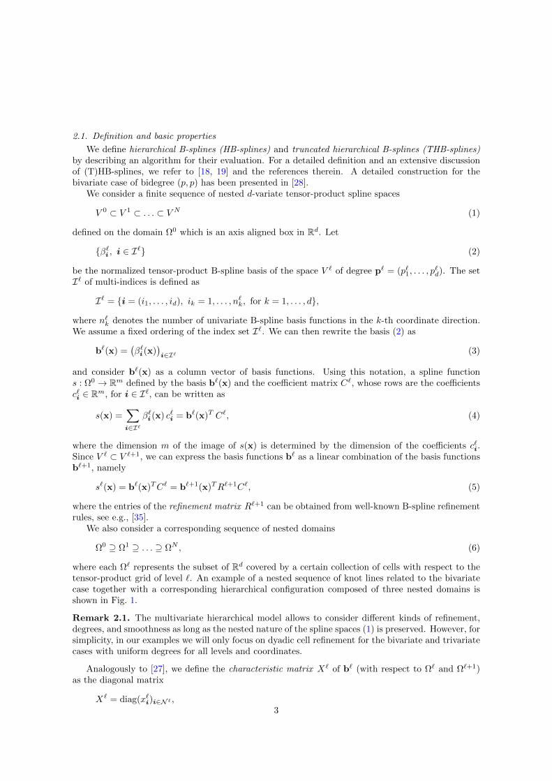
(a) B-splines of level 0 (b) HB-splines of level 0

(c) B-splines of level 1 (d) HB-splines of level 1 (e) THB-splines of level 0after truncation with re-spect to level 1

(f) THB-splines on 2 lev-els: union of functionsin (d) and (e)

(g) B-splines of level 2 (h) HB-splines of level 2 (i) THB-splines of level 0and 1 after truncation withrespect to level 2

(j) THB-splines on 3 levels:union of functions in (h)and (i)

Figure 3: Illustration of THB-spline basis construction on the domain hierarchy shown in Figure 1. The basis functionsare displayed all at once in a top-down view. Note that, while HB-splines at level 2 are given by the union of functionsin (b), (c), and (d), THB-splines at level 2 are given by the union of functions in (h) and (i), see also (j).

Note that in the THB-spline evaluation (b) in Algorithm 1 we explicitly use identity (11) tostress that each intermediate coefficient of level ` is either obtained by refinement from intermediatecoefficients of the previous level, or it is a coefficient of the THB-spline representation (9). Thealgorithm implicitly defines the (T)HB-basis functions τ `i , (`, i) ∈ I, since one can obtain the valueof τ `i by applying the algorithm to a characteristic coefficient matrix. More precisely, if the algorithmis applied to evaluate a (T)HB-spline function s as in (9) at a point x, the computations will berestricted only to the B-spline basis functions which contain x in their support. Furthermore, due to(12), the loop in Algorithm 1 will not necessarily go through all levels from 0 to N , but only up tolevel ` when x ∈ Ω` \ Ω`+1.

6

2.2. Implementation in G+++SMO

We describe an efficient C++ implementation of THB-splines, which is a module of the G+++SMOlibrary1. The implementation extends the prior 2D implementation presented in [27] to arbitraryspatial dimension d. This code is used for all examples presented in the present paper.

G+++SMO is an open-source, object-oriented C++ library for isogeometric analysis. The librarymakes use of object polymorphism and inheritance techniques in order to support a variety of dif-ferent discretization bases, namely B-spline, Bernstein, NURBS bases, hierarchical and truncatedhierarchical B-spline bases of arbitrary polynomial order. The implementation of basis functions andgeometries is dimension-independent, that is, curves, surfaces, volumes, bulks (in 4D) and other high–dimensional objects are instances of code templated with respect to the parameter domain dimension.

Three general guidelines have been set for the development process. Firstly, we promote bothefficiency and ease of use; secondly, we ensure code quality and cross-platform compatibility and,thirdly, we always explore new strategies better suited for isogeometric analysis before adopting FEMpractices.

The library is partitioned into modules that implement different functionalities. A basic modulethat is available is the NURBS module, which provides a dimension independent implementation ofclassical tensor-product B-splines and their rational counterpart. On top of the NURBS module weimplemented the hierarchical splines module, which shall be described in more detail in the sequel.

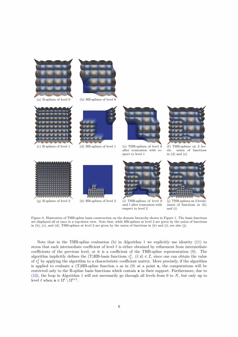
The hierarchical domain. The backbone of the (T)HB-splines implementation is a suitable represen-tation of the hierarchical domain. This is realized using a binary subdivision tree data structure,which is a generalization of the quad-tree implementation of [27]. The leaves of this tree form apartition of the domain into quadrilateral (in 2D) or cubical (in 3D) subdomains with the propertythat each subdomain (which is a collection of domain cells) is contained in the same hierarchical level.This allows for fast queries to be implemented, for instance identifying the level of an input cell, orreporting all cells that overlap a given quadrilateral.

In Figure 4 we show an instance of the hierarchical data structure corresponding to the domain ofFigure 1. The domain data in this tree are represented by long integers. These refer to knot indicesof the corresponding level. Each interior node (circles in Figure 4) stores a split position and the axisindex along which the splitting is performed. Leaf nodes (that is, squares in Figure 4) do not storesplit position or axis, but they store a level index as well as the corner coordinates of the subdomainthat it represents.

Note that the leaves are rectangular collections of elements of the same level. The representationsof these rectangular subdomains are stored using distinct knot indices. This has the advantage ofavoiding numerical errors, even on high levels. Also, note that knot indices on levels higher than zerohave the form 2`κ where κ is an index of a distinct knot in level zero. This allows to perform allrelated computations by low-level bit operations which are highly efficient. For instance, convertingthe knot indices between different hierarchical level requires multiplication or division by powers oftwo, since we restrict ourselves to dyadic refinement. Bit-shift operations provide an efficient way toimplement these conversions.

The hierarchical data structure is initialized by the initial tensor-product mesh Ω0 as in Figure 1(a).Then an insertion operation can be used to insert new subdomains in the hierarchy. Furthermore theset of active basis functions and the corresponding characteristic matrices X` for all levels ` can beefficiently extracted. This is done during a basis compilation (or initialization) step, after the boxinsertion.

Basis compilation step. After constructing the hierarchical domain, a basis compilation step takesplace. In this step, the characteristic matrices X` for all levels ` are constructed and stored in asparse format.

1Geometry + Simulation Modules, gs.jku.at/gismo

7

gs.jku.at/gismo

1

2

3

4

5

6

7

8

9

A B

C D

E

F

G

H

I

J

1

2 3

4 5 6 7

8 9 E F G H I J

A B C D

Figure 4: The partition of a domain and the binary subdivision tree for the example in Figure 1 (mesh on the left).

In the case of THB-splines, we identify the subset of basis functions that need to be truncated.This is done by a support overlap query on the tree structure. For an efficient evaluation procedure,we proceed as follows: for a truncated basis function, we identify the coarsest level `c such that itadmits a representation in terms of B-spline functions of that level. This extra information is collectedduring the support overlap query. Consequently, we precompute and store this representation in level`c in order to speed up subsequent evaluations. This computation is done according to Algorithm 1,by setting all input coefficients C` to 0 except for the coefficient of the desired basis function whichis set to 1 and then iterating for all levels N ≤ `c. The algorithm has then to be executed only once,and subsequent function evaluations are reduced to computing linear combinations of (typically few)tensor-product B-spline basis functions.

For storage and data exchange we do not need to store the precomputed B-spline representationsof the truncated basis functions, as this information can always be recomputed from the domain hi-erarchy or from the characteristic matrices. Thus, using THB-splines does not increase the requiredmemory for storage and data exchange. When performing computations and evaluations, however,the precomputation of THB-splines, which increases the efficiency, leads to additional memory con-sumption, see the experimental results reported below. For sufficient mesh grading, the memory stillgrows linearly with the number of degrees of freedom, see Fig. 7.

Point-wise evaluation of basis functions and (T)HB-splines. The evaluation of a tensor-product B-spline basis function in a HB-spline or THB-spline basis is done via the recursive definition. For atruncated basis function we use the precomputed coefficients to obtain its value as a linear combinationof tensor-product B-splines at the representation level `c.

If all active basis functions at the given point are requested, it is often the case that several ofthem possess the same representation level. In this case, we exploit this fact by caching the values ofactive B-splines at the representation level, in order to increase efficiency.

The evaluation of a field at given point is performed by Algorithm 1. The implementation takesinto account the level of a point and stops the iterations there. Without precomputation of the B-splinerepresentation of the truncated basis functions, the cost of the THB–spline evaluation is equal to theapplication of the B-spline subdivision rule (“level of a point” times) plus the cost of the standard deBoor’s algorithm, see also [27] for a detailed discussion. When using precomputation, this is reducedto the cost of the standard de Boor’s algorithm.

Adaptive refinement: box insertion. Inserting boxes into the domain structure is the basic tool forperforming adaptive refinement. It takes place as soon as subdomains need to be added in levels higherthan zero. Firstly, quadrilateral subdomains are inserted at higher levels in the binary subdivisiontree. Secondly, the resulting domain structure is used to update locally the characteristic matrices.

In the first step, new nodes are created with split positions and axes adapted to the input box.More precisely, the new box is tracked from the root of the tree until the leaves, and all overlapping

8

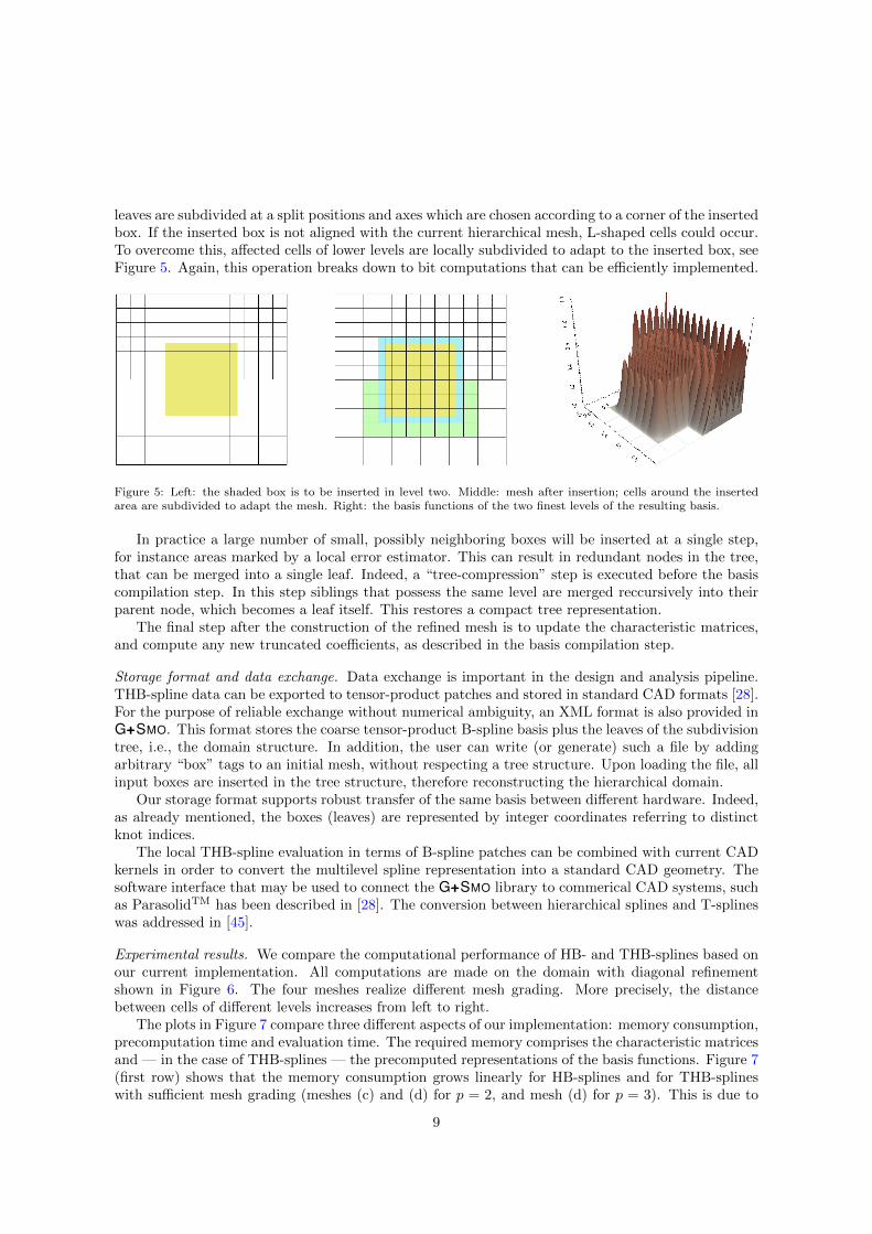
leaves are subdivided at a split positions and axes which are chosen according to a corner of the insertedbox. If the inserted box is not aligned with the current hierarchical mesh, L-shaped cells could occur.To overcome this, affected cells of lower levels are locally subdivided to adapt to the inserted box, seeFigure 5. Again, this operation breaks down to bit computations that can be efficiently implemented.

Figure 5: Left: the shaded box is to be inserted in level two. Middle: mesh after insertion; cells around the insertedarea are subdivided to adapt the mesh. Right: the basis functions of the two finest levels of the resulting basis.

In practice a large number of small, possibly neighboring boxes will be inserted at a single step,for instance areas marked by a local error estimator. This can result in redundant nodes in the tree,that can be merged into a single leaf. Indeed, a “tree-compression” step is executed before the basiscompilation step. In this step siblings that possess the same level are merged reccursively into theirparent node, which becomes a leaf itself. This restores a compact tree representation.

The final step after the construction of the refined mesh is to update the characteristic matrices,and compute any new truncated coefficients, as described in the basis compilation step.

Storage format and data exchange. Data exchange is important in the design and analysis pipeline.THB-spline data can be exported to tensor-product patches and stored in standard CAD formats [28].For the purpose of reliable exchange without numerical ambiguity, an XML format is also provided inG+++SMO. This format stores the coarse tensor-product B-spline basis plus the leaves of the subdivisiontree, i.e., the domain structure. In addition, the user can write (or generate) such a file by addingarbitrary “box” tags to an initial mesh, without respecting a tree structure. Upon loading the file, allinput boxes are inserted in the tree structure, therefore reconstructing the hierarchical domain.

Our storage format supports robust transfer of the same basis between different hardware. Indeed,as already mentioned, the boxes (leaves) are represented by integer coordinates referring to distinctknot indices.

The local THB-spline evaluation in terms of B-spline patches can be combined with current CADkernels in order to convert the multilevel spline representation into a standard CAD geometry. Thesoftware interface that may be used to connect the G+++SMO library to commerical CAD systems, suchas ParasolidTM has been described in [28]. The conversion between hierarchical splines and T-splineswas addressed in [45].

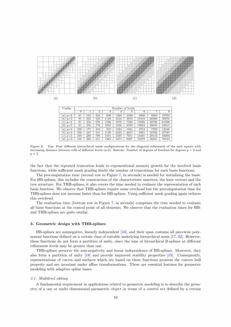
Experimental results. We compare the computational performance of HB- and THB-splines based onour current implementation. All computations are made on the domain with diagonal refinementshown in Figure 6. The four meshes realize different mesh grading. More precisely, the distancebetween cells of different levels increases from left to right.

The plots in Figure 7 compare three different aspects of our implementation: memory consumption,precomputation time and evaluation time. The required memory comprises the characteristic matricesand — in the case of THB-splines — the precomputed representations of the basis functions. Figure 7(first row) shows that the memory consumption grows linearly for HB-splines and for THB-splineswith sufficient mesh grading (meshes (c) and (d) for p = 2, and mesh (d) for p = 3). This is due to

9

(a) (b) (c) (d)

Config. Number of levels0 1 2 3 4 5 6 7 8

(a) p=2 81 164 324 638 1260 2498 4968 9902 19764(b) p=2 81 222 524 1148 2416 4972 10104 20388 40976(c) p=2 81 256 676 1586 3476 7326 15096 30706 61996(d) p=2 81 256 770 1942 4430 9550 19934 40846 82814

(a) p=3 100 177 310 555 1024 1941 3754 7359 14548(b) p=3 100 247 541 1129 2305 4657 9361 18769 37585(c) p=3 100 289 709 1591 3397 7051 14401 29143 58669(d) p=3 100 289 811 1963 4375 9307 19279 39331 79543

Figure 6: Top: Four different hierarchical mesh configurations for the diagonal refinement of the unit square withincreasing distance between cells of different levels (a-d). Bottom: Number of degrees of freedom for degrees p = 2 andp = 3.

the fact that the repeated truncation leads to exponentional memory growth for the involved basisfunctions, while sufficient mesh grading limits the number of truncations for each basis functions.

The precomputation time (second row in Figure 7, in seconds) is needed for initializing the basis.For HB-splines, this includes the construction of the characteristic matrices, the knot vectors and thetree structure. For THB-splines, it also covers the time needed to evaluate the representation of eachbasis function. We observe that THB-splines require some overhead but the precomputation time forTHB-splines does not increase faster than for HB-splines. Using sufficient mesh grading again reducesthis overhead.

The evaluation time (bottom row in Figure 7, in seconds) comprises the time needed to evaluateall basis functions at the central point of all elements. We observe that the evaluation times for HB-and THB-splines are quite similar.

3. Geometric design with THB-splines

HB-splines are nonnegative, linearly independent [43], and their span contains all piecewise poly-nomial functions defined on a certain class of suitable underlying hierarchical mesh [17, 32]. However,these functions do not form a partition of unity, since the sum of hierarchical B-splines at differentrefinement levels may be greater than one.

THB-splines preserve the non-negativity and linear independence of HB-splines. Moreover, theyalso form a partition of unity [18] and provide improved stability properties [19]. Consequently,representations of curves and surfaces which are based on these functions prossess the convex hullproperty and are invariant under affine transformations. These are essential features for geometricmodeling with adaptive spline bases.

3.1. Multilevel editing

A fundamental requirement in applications related to geometric modeling is to describe the geom-etry of a one or multi–dimensional parametric object in terms of a control net defined by a certain

10

1.5 2.0 2.5 3.0 3.5 4.0 4.5 5.0

log(DOF)

2

3

4

5

6

7

8

log(

Mem

ory)

1

1

Degree 2

2.0 2.5 3.0 3.5 4.0 4.5 5.0

log(DOF)

2

3

4

5

6

7

8

log(

Mem

ory)

Degree 3

0 1 2 3 4 5 6 7 8

Levels−3.5

−3.0

−2.5

−2.0

−1.5

−1.0

−0.5

0.0

0.5

1.0

log(

Pre

com

puta

tion

tim

e)

Degree 2

0 1 2 3 4 5 6 7 8

Levels−3.5

−3.0

−2.5

−2.0

−1.5

−1.0

−0.5

0.0

0.5

1.0

log(

Pre

com

puta

tion

tim

e)

Degree 3

0 1 2 3 4 5 6 7 8

Levels−4.0

−3.5

−3.0

−2.5

−2.0

−1.5

−1.0

−0.5

0.0

0.5

log(

Eva

luat

ion

tim

e)

Degree 2

0 1 2 3 4 5 6 7 8

Levels−3.5

−3.0

−2.5

−2.0

−1.5

−1.0

−0.5

0.0

0.5

1.0

log(

Eva

luat

ion

tim

e)

Degree 3

Figure 7: Experimental results for HB-splines (solid lines) and THB-splines (dashed lines) for the four hierarchical meshconfigurations shown in Figure 6. The brown, red, green and blue color corresponds to the meshes (a-d), respectively.

collection of points. Consequently, manipulations of the parametric shape can be replaced by anal-ogous (but simpler) operations on this modeling tool. In order to achieve this, any point along theparametric form p is represented as a convex linear combination of the considered control points dì interms of nonnegative basis functions which satisfy the partition of unity property,

p(x) =∑

(i,`)∈I

dìτì (x).

The generalization to rational forms is also possible and analogous to NURBS curves and surfaces.The convex hull property of THB-splines allows us to introduce the concept of a multilevel control

structure, defined by the set of control points (and the edges connecting them) associated to thetruncated basis function level by level. The three following examples show how this hierarchicalcontrol tool can be effectively used to perform interactive editing and design.

11

Example 1. In the univariate case, B-spline geometries can easily be manipulated through interactiveand local editing of their control polygons without the need of additional extensions to hierarchicalconfigurations. Nevertheless, in order to start with a simple example, we consider the successivemodification of a B-spline curve according to a hierarchical control structure that consists of 4 differentrefinement levels in Figure 8. The control structure is shown in the top row. The HB- and THB-splinecurves defined by considering the set of control points up to level 2, 3, and 4 are shown from left toright in Figure 8(b) and (c), respectively.

Since HB-splines do not form a convex partition of unity, the curve is not confined to the convexhull. Moreover, it is not affinely invariante, hence even a simple translation of the curve would producea different curve. In contrast, the THB-spline representation is suitable for geometric modeling.The curve is contained in the convex hull of the corresponding multilevel control polygon and therepresentation is invariant under affine transformations.

3 4 5 6 7 81

1.5

2

2.5

(a) multilevel control polygon with four levels

5 10 15 20 25

2

4

6

5 10 15 20 25

2

4

6

5 10 15 20 25

2

4

6

5 10 15 20 25

2

4

6

(b) HB-spline curve on 1-4 levels (from left to right)

3 4 5 6 7 81

1.5

2

2.5

3 4 5 6 7 81

1.5

2

2.5

3 4 5 6 7 81

1.5

2

2.5

3 4 5 6 7 81

1.5

2

2.5

(c) THB-spline curve on 1-4 levels (from left to right)

Figure 8: Comparison of HB-spline (b) and THB-spline (c) representations at different refinement levels obtained byapplying multilevel editing to the same initial B-spline curve and corresponding control polygon (a).

Example 2. We now present an example for local multilevel editing in the bivariate case. We startby considering the wine-glass-shaped B-spline surface shown on top the left of Figure 9. Several subse-quent refinement levels are considered: the locally refined hierarchical meshes and the correspondingmultilevel control nets defining the same THB-spline geometry are there shown (top center). In orderto modify the bowl of the glass without propagation to the stem or the foot, we exploit the localnature of adaptive THB-spline refinements, which allows to insert additional control points only inthe upper part of the model (middle row). Subsequently, these newly inserted control points can beinteractively moved to change the shape of the bowl and insert an additional local feature (top rightand bottom right). Using the standard tensor-product B-spline representation would have required aglobal refinement of the mesh.

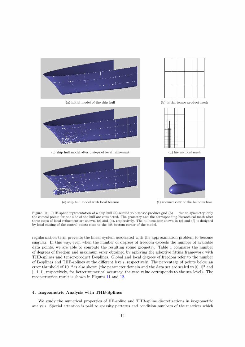
Example 3. As second bivariate example of adaptive modeling, we present the editing of the bulbousbow at the front of a ship. Figures 10(a) and 10(b) illustrate the initial ship hull and the correspondingtensor-product grid, Figure 10(c) and 10(d) show the locally refined geometry and the hierarchicalmesh after three refinement steps. In order to model the bulbous bow at the front of the ship, thecontrol points on the left bottom corner are suitably changed, see Figures 10(e) and 10(f). Note that

12

Figure 9: THB-spline representations of a wine glass (top row) using three different hierarchical meshes in the parameterdomain (middle row). The images of the knot lines in the hierarchical mesh exhibit T-joints on the surface (bottomleft). The THB-spline control mesh is suitable for interactive shape editing (bottom right).

the control net shown in (c) and (e) has 193 control points. Three steps of global refinement wouldlead to 1300 degrees of freedom.

3.2. Reconstruction of geographic data

Adaptive spline models may be suitably exploited also for an effective reconstruction of complexmodels starting from large data sets. For example, the use of LR spline representation in the contextof geographical data approximation has been recently addressed [41]. The next example demonstratesthat adaptive refinement with hierarchical splines allows to obtain high accuracy with a reducednumber of degrees of freedom when compared to classical tensor-product approximations.

Example 4. In order to compare the adaptive behaviour of hierarchical constructions with the uni-form B-spline scheme, we compute a regularized least squares approximation in terms of THB–splines[28] for the Baltic sea data set iowtopo1 consisting of 133,200 (spherical) gridded data points2. The

2 The data set is available at www.io-warnemuende.de/topography-of-the-baltic-sea.html (Leibniz Institute forBaltic Sea Research Warnemunde, Digital Topography of the Baltic Sea).

13

www.io-warnemuende.de/topography-of-the-baltic-sea.html

(a) initial model of the ship hull (b) initial tensor-product mesh

(c) ship hull model after 3 steps of local refinement (d) hierarchical mesh

(e) ship hull model with local feature (f) zoomed view of the bulbous bow

Figure 10: THB-spline representation of a ship hull (a) related to a tensor-product grid (b) — due to symmetry, onlythe control points for one side of the hull are considered. The geometry and the corresponding hierarchical mesh afterthree steps of local refinement are shown, (c) and (d), respectively. The bulbous bow shown in (e) and (f) is designedby local editing of the control points close to the left bottom corner of the model.

regularization term prevents the linear system associated with the approximation problem to becomesingular. In this way, even when the number of degrees of freedom exceeds the number of availabledata points, we are able to compute the resulting spline geometry. Table 1 compares the numberof degrees of freedom and maximum error obtained by applying the adaptive fitting framework withTHB-splines and tensor-product B-splines. Global and local degrees of freedom refer to the numberof B-splines and THB-splines at the different levels, respectively. The percentage of points below anerror threshold of 10−3 is also shown (the parameter domain and the data set are scaled to [0, 1]2 and[−1, 1], respectively, for better numerical accuracy, the zero value corresponds to the sea level). Thereconstruction result is shown in Figures 11 and 12.

4. Isogeometric Analysis with THB-Splines

We study the numerical properties of HB-spline and THB-spline discretizations in isogeometricanalysis. Special attention is paid to sparsity patterns and condition numbers of the matrices which

14

refinement step no. of degrees of freedom maximum error % below thresholdlocal global local global local global

0 100 100 1.02e-01 1.02e-01 10.44 10.441 324 324 9.59e-02 9.59e-02 16.58 16.582 1,156 1,156 8.68e-02 8.68e-02 27.62 27.623 4,356 4,356 6.82e-02 6.82e-02 41.23 41.234 16,398 16,900 6.38e-02 6.38e-02 57.62 57.635 57,034 66564 2.79e-02 2.79e-02 77.24 77.296 164,011 264,196 6.27e-03 6.27e-03 98.58 98.83

Table 1: Number of local (hierarchical) and global (tensor-product) degrees of freedom and related maximum error withrespect to different refinement steps obtained by sampling 133,200 data points from the Baltic sea data set consideredin Example 4. The percentage of points (%) below the error threshold of 10−3 is also shown.

Figure 11: THB-spline approximations of the baltic sea data set considered in Example 4 at step 0, 3 and 6 (top row andbottom left). The corresponding multilevel control mesh at level 6 is also shown (bottom right). The different colorsidentify the control meshes of the different levels, where the color varies from red to dark blue as the level increases.

need to be generated when solving PDEs using Galerkin discretization. A comparison between HB-splines, THB-splines, and LR splines was recently presented in [24]. The results of the following

15

Figure 12: Close-up view at adaptive reconstruction of the Lolland and Falster islands, Denmark.

examples extend the analysis for the hierarchical case to more complex geometries, 3D configurations,and different model problems.

4.1. Model problem and discretization

We will consider several model problems, namely the Laplace equation, the Poisson equation, andadvection-diffusion problems. These problems can be written in the following general form:

Find u ∈ V = C2(Ω) ∩ C(Ω), such that

Lu = f in Ω,u = gD on ∂Ω,

(13)

where L is an elliptic second-order differential operator. In order to keep the presentation concise werestrict ourselves to Dirichlet boundary conditions.

By using standard techniques, we reformulate (13) in the following variational form:

Find u ∈ Vg ⊂ V = H1(Ω), such that a(u, v) = 〈f, v〉, ∀v ∈ V0 ⊂ V, (14)

where a(·, ·) and 〈f, ·〉 are the bilinear form and the linear functional induced by the considered PDE,V0 denotes the space of test functions which vanish on the Dirichlet boundary, and where Vg is theset of functions fulfilling the Dirichlet boundary conditions.

Using Galerkin discretization, we obtain from (14) the linear system of equations

Lh uh = fh. (15)

We refer to Lh as system matrix, and to fh as load vector. Solving system (15), we obtain the coefficientvector uh, which defines the discrete solution uh. The system (15) is typically large and sparse, andit is solved by an iterative solver. The performance and convergence rate of such iterative solversdepends, amongst other factors, on the sparsity and on the condition number of the system matrixLh (see, e.g., [37]).

The discretization space is constructed by employing the isogeometric approach [9]: Given a ge-ometry mapping F : Ω′ → Ω that maps the parameter domain Ω′ to the physical domain Ω, thediscretization space is spanned by the isogeometric functions

Bì = Bì F−1 i.e. Bì(F (ξ)) = Bì(ξ) ∀ξ ∈ Ω′, (16)16

where the basis functions Bì are (truncated) hierarchical B-splines (or rational versions thereof),Bì = βì or Bì = τ ì , see Section 2. It is also assumed that the geometry mapping F admits arepresentation in the same space, thereby complying with the isoparametric principle.

In the numerical examples presented below we will report and compare the condition numbers andnumber of non-zero entries related to Lh, or the mass matrix Mh and the stiffness matrix Kh,

(Mh)(i,`),(j,k) = (Bì , Bkj )L2

=

∫Ω

BìBkj dx, (Kh)(i,`)(j,k) =

∫Ω

∇Bì · ∇Bkj dx, (i, `), (j, k) ∈ I,

(17)

for HB- or THB-splines, namely for Bì = βì or Bì = τ ì . Note that the values reported in thecolumn labeled “# d.o.f.” of the following tables refer to the total number of degrees of freedomof the corresponding discrete space. All other values (i.e., numbers of non-zero entries, bandwidth,and condition numbers) are computed after elimination of all degrees of freedom associated with theDirichlet boundary.

4.2. Ad hoc refinement

In the first two examples, we apply ad hoc refinement on the unit hypercube, i.e., Ω = (0, 1)d,d = 2, 3, which is discretized with HB- and THB-splines of degrees p = 2, 3, 4 using the identity asthe geometry mapping.

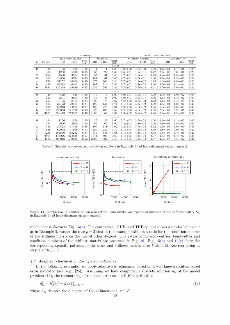
Example 5 (Ad hoc refinement on unit square). We consider the discretization of the unit square,i.e., Ω = (0, 1)2, with Cp−1-smooth HB- and THB-splines of degrees p = 2, 3, 4. Fig. 13 shows thehierarchical meshes after 5 steps of refinement in a strip of 2p+ 1 cells centered at the diagonal.

Table 2 reports the numbers of hierarchical levels and degrees of freedom (d.o.f.) associated tothe considered meshes in the columns labeled “L” and “#d.o.f.”, respectively. The numbers of non-zero entries, the bandwidth, and the condition numbers of mass and stiffness matrices are presentedtogether with their ratios, provided in the column labeled “THB

HB ”. These ratios are also visualized inthe plots shown in Fig. 14. Note that these ratios are computed before rounding, i.e., the ratios ofthe presented numbers may slightly differ from the reported ratios. These results show that the useof THB-splines significantly reduces the number of non-zero entries. The condition numbers are alsoeither improved or possess the same order of magnitude, except the case p = 2 related to the stiffnessmatrix.

(a) p = 2 (b) p = 3 (c) p = 4

Figure 13: Meshes after 5 steps of refinement in Example 5 (ad hoc refinement on unit square).

Example 6 (Ad hoc refinement on unit cube). We consider the discretization of the unit cubeΩ = (0, 1)3 with HB- and THB-splines of degrees p = 2, 3, 4 and global Cp−1 smoothness. We refinealong a layer that is defined by a sphere of radius 0.5, centered at the origin. All cells overlapping thissphere, as well as one layer of cells around those, are refined in each step. The mesh after 3 steps of

17

sparsity condition numbersnon-zero entries bandwidth stiffness matrix mass matrix

L #d.o.f. HB THB THBHB HB THB THB

HB HB THB THBHB HB THB THB

HB

p = 20 36 196 196 1.00 11 11 1.00 4.0e+00 4.0e+00 1.00 4.1e+01 4.1e+01 1.001 86 1208 1030 0.85 35 22 0.63 2.6e+01 1.1e+01 0.42 2.6e+02 6.0e+01 0.232 180 4580 3304 0.72 85 41 0.48 3.7e+01 1.8e+01 0.49 8.4e+02 1.8e+02 0.223 362 13856 8734 0.63 181 81 0.45 4.7e+01 4.7e+01 1.00 3.2e+03 7.2e+02 0.224 720 37252 20800 0.56 375 160 0.43 5.7e+01 1.1e+02 1.93 1.3e+04 2.9e+03 0.225 1430 93312 46462 0.50 767 310 0.40 6.7e+01 2.4e+02 3.60 5.2e+04 1.1e+04 0.226 2844 223348 99640 0.45 1555 599 0.39 7.7e+01 5.1e+02 6.61 2.1e+05 4.6e+04 0.22



Table 2: Sparsity properties and condition numbers in Example 5 (ad hoc refinement on unit square).

2000 4000 60000

0.5

1

# d.o.f.

rati

oT

HB

/H

B

non-zero entries

p = 2

p = 3

p = 4

2000 4000 60000

0.5

1

# d.o.f.

rati

oT

HB

/H

B

bandwidth

p = 2

p = 3

p = 4

2000 4000 60000

2

4

6

8

# d.o.f.

rati

oT

HB

/H

B

condition number Kh

p = 2

p = 3

p = 4

Figure 14: Comparison of number of non-zero entries, bandwidths, and condition numbers of the stiffness matrix Kh

in Example 5 (ad hoc refinement on unit square).

refinement is shown in Fig. 15(a). The comparison of HB- and THB-splines shows a similar behaviouras in Example 5, except the case p = 2 that in this example exhibits a ratio for the condition numberof the stiffness matrix on the line of other degrees. The ratios of non-zero entries, bandwidths andcondition numbers of the stiffness matrix are presented in Fig. 16. Fig. 15(b) and 15(c) show thecorresponding sparsity patterns of the mass and stiffness matrix after Cuthill-McKee-reordering atstep 3 with p = 2.

4.3. Adaptive refinement guided by error estimates

In the following examples, we apply adaptive h-refinement based on a well-known residual-basederror indicator (see, e.g., [25]). Assuming we have computed a discrete solution uh of the modelproblem (13), the estimate ηK of the local error on a cell K is defined as

η2K = h2

K‖f − Luh‖2L2(K), (18)

where hK denotes the diameter of the d-dimensional cell K.18

(a) mesh of the physical domain (b) HB-splines (c) THB-splines

Figure 15: Mesh (a) and sparsity patterns of mass and stiffness matrix (after Cuthill-McKee-reordering) related to HB-(b) and THB-splines (c) in Example 6 for p = 2 (ad hoc refinement on unit cube) at step 3.

2000 4000 6000

0.5

1

# d.o.f.

rati

oT

HB

/H

B

non-zero entries

p = 2

p = 3

p = 4

2000 4000 6000

0.5

1

# d.o.f.

rati

oT

HB

/H

B

bandwidth

p = 2

p = 3

p = 4

2000 4000 6000

0.5

1

# d.o.f.

rati

oT

HB

/H

B

condition number Kh

p = 2

p = 3

p = 4


in Example 6 (ad hoc refinement on unit cube).

Remark 4.1. Note that residual-based error indicators also involve a term corresponding to thejumps of ∇uh across cell interfaces, and a term involving Neumann boundary conditions. Both termsvanish when considering at least C1-continuous discrete solutions and Dirichlet boundary conditions.

A cell K is marked for refinement, if the criterion

ηK ≥ Θ (19)

is fulfilled for a threshold Θ. We use two different strategies for choosing this threshold, which wedescribe in the following. These strategies depend on a scalar parameter ψ ∈ [0, 1], where the choicesψ ≈ 0 and ψ ≈ 1 result in global and no refinement, respectively.

(i) “Absolute threshold”: We compute Θ as

Θ = ψ ·maxKηK, ψ ∈ [0, 1]. (20)

Note that the percentage of marked cells may vary in each step, since the threshold computa-tion only takes into account the magnitude of the largest local error, without considering thedistribution of the estimated error.

(ii) “Relative threshold”: We fix a percentage of all cells that should be marked in each step, bychoosing Θ such that

|K : ηK > Θ| ≈ (1− ψ) · |K|19

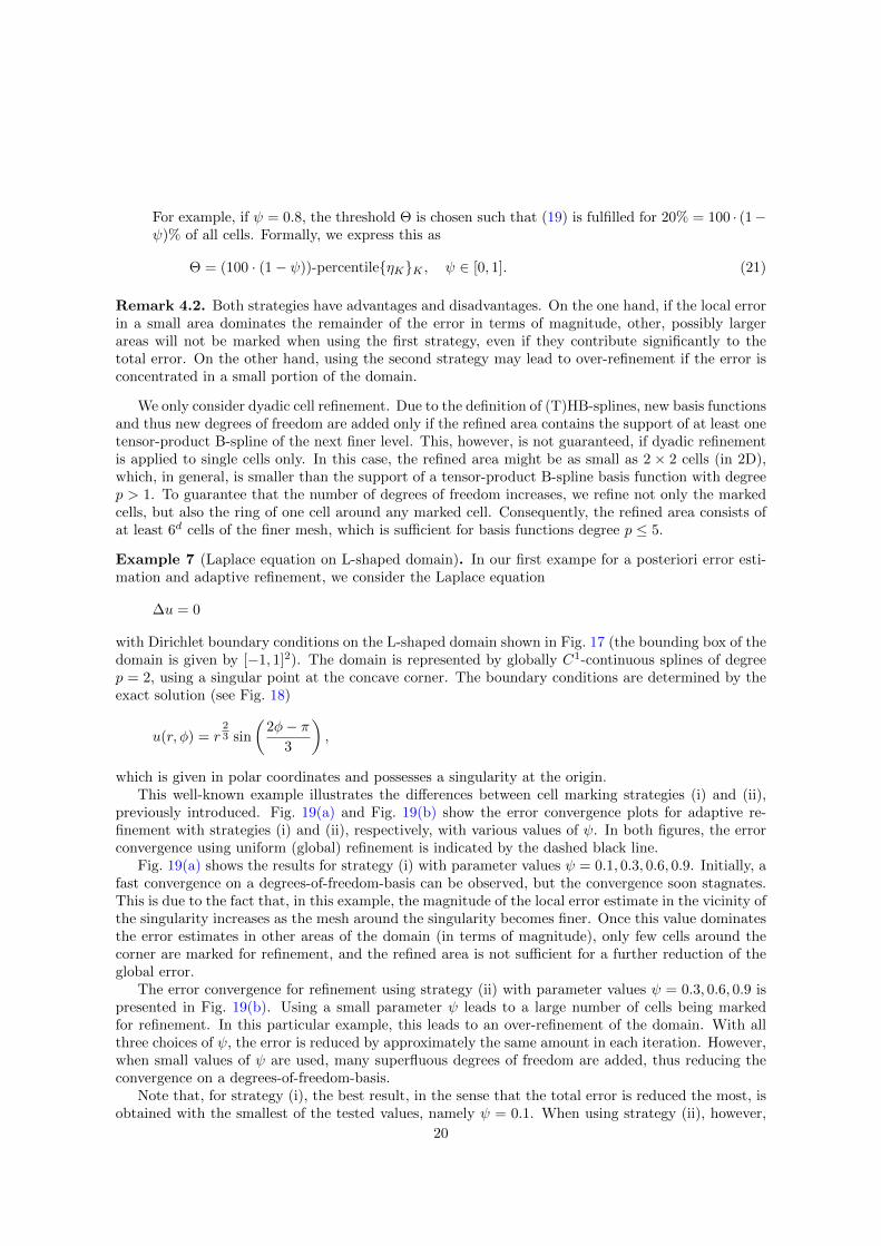
For example, if ψ = 0.8, the threshold Θ is chosen such that (19) is fulfilled for 20% = 100 · (1−ψ)% of all cells. Formally, we express this as

Θ = (100 · (1− ψ))-percentileηKK , ψ ∈ [0, 1]. (21)

Remark 4.2. Both strategies have advantages and disadvantages. On the one hand, if the local errorin a small area dominates the remainder of the error in terms of magnitude, other, possibly largerareas will not be marked when using the first strategy, even if they contribute significantly to thetotal error. On the other hand, using the second strategy may lead to over-refinement if the error isconcentrated in a small portion of the domain.

We only consider dyadic cell refinement. Due to the definition of (T)HB-splines, new basis functionsand thus new degrees of freedom are added only if the refined area contains the support of at least onetensor-product B-spline of the next finer level. This, however, is not guaranteed, if dyadic refinementis applied to single cells only. In this case, the refined area might be as small as 2 × 2 cells (in 2D),which, in general, is smaller than the support of a tensor-product B-spline basis function with degreep > 1. To guarantee that the number of degrees of freedom increases, we refine not only the markedcells, but also the ring of one cell around any marked cell. Consequently, the refined area consists ofat least 6d cells of the finer mesh, which is sufficient for basis functions degree p ≤ 5.

Example 7 (Laplace equation on L-shaped domain). In our first exampe for a posteriori error esti-mation and adaptive refinement, we consider the Laplace equation

∆u = 0

with Dirichlet boundary conditions on the L-shaped domain shown in Fig. 17 (the bounding box of thedomain is given by [−1, 1]2). The domain is represented by globally C1-continuous splines of degreep = 2, using a singular point at the concave corner. The boundary conditions are determined by theexact solution (see Fig. 18)

u(r, φ) = r23 sin

(2φ− π

3

),

which is given in polar coordinates and possesses a singularity at the origin.This well-known example illustrates the differences between cell marking strategies (i) and (ii),

previously introduced. Fig. 19(a) and Fig. 19(b) show the error convergence plots for adaptive re-finement with strategies (i) and (ii), respectively, with various values of ψ. In both figures, the errorconvergence using uniform (global) refinement is indicated by the dashed black line.

Fig. 19(a) shows the results for strategy (i) with parameter values ψ = 0.1, 0.3, 0.6, 0.9. Initially, afast convergence on a degrees-of-freedom-basis can be observed, but the convergence soon stagnates.This is due to the fact that, in this example, the magnitude of the local error estimate in the vicinity ofthe singularity increases as the mesh around the singularity becomes finer. Once this value dominatesthe error estimates in other areas of the domain (in terms of magnitude), only few cells around thecorner are marked for refinement, and the refined area is not sufficient for a further reduction of theglobal error.

The error convergence for refinement using strategy (ii) with parameter values ψ = 0.3, 0.6, 0.9 ispresented in Fig. 19(b). Using a small parameter ψ leads to a large number of cells being markedfor refinement. In this particular example, this leads to an over-refinement of the domain. With allthree choices of ψ, the error is reduced by approximately the same amount in each iteration. However,when small values of ψ are used, many superfluous degrees of freedom are added, thus reducing theconvergence on a degrees-of-freedom-basis.

Note that, for strategy (i), the best result, in the sense that the total error is reduced the most, isobtained with the smallest of the tested values, namely ψ = 0.1. When using strategy (ii), however,

20

the fastest convergence on a degrees-of-freedom-basis is achieved by the largest value of ψ, namelyψ = 0.9. For this reason, we will compare the results obtained with these two configurations: strategy(i), ψ = 0.1, and strategy (ii), ψ = 0.9.

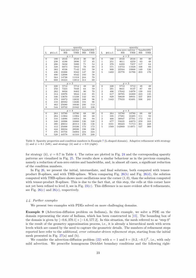
The adaptively refined meshes obtained with these two strategies are compared in Fig. 17, andthe corresponding sparsity patterns (after Cuthill-McKee-reordering) of mass and stiffness matricesare shown in Fig. 20. The computed numbers of non-zero matrix entries, bandwidths, and conditionnumbers are reported in Table 3, while the THB vs HB ratios are presented in Fig. 21 and 22. Wealso present the numbers for discretizations of degrees 3 and 4, i.e., for the computations carried outafter applying one or two steps of p-refinement on the geometry mapping and thus on the initial mesh(see, e.g., [9, 10]).

In all tested settings, the use of THB-splines results in a (in some cases substantial) reduction ofthe number of non-zero matrix entries, and of the bandwidth, compared to HB-splines. The conditionnumbers of the stiffness and mass matrix are either improved or increased only moderately.

(a) parameter and physical domains — strategy (i) (b) parameter and physical domains — strategy (ii)

Figure 17: Adaptively refined meshes in Example 7 (L-shaped domain). The hierarchical configurations obtained after8 refinements with strategy (i), ψ = 0.1 (a) and after 5 refinements with strategy (ii), ψ = 0.9 (b) are shown.

Figure 18: Computed solution in Example 7 (L-shaped domain). A comparison of initial and final solutions is omitted,because the differences are too small to be visible.

Example 8 (Advection-diffusion problem on unit square). This example is also well-known in thecontext of adaptive refinement and has already been used in numerous publications on isogeometricanalysis, e.g., [9, 22]. We consider an advection-diffusion-problem of the form

−κ∆u+ b · ∇u = 0, (22)

where κ = 10−6 is the diffusion coefficient, and the advection velocity is given by b = (cos π4 , sinπ4 )T .

The Peclet number Pe is defined by Pe = L|b|/κ, where L is the side length of the domain. If Pe 1,the advection dominates the diffusion, which is clearly the case in our example with Pe ≈ 106. TheStreamline Upwinding Petrov Galerkin (SUPG) stabilization method is used for stabilization, i.e., we

21

102 103

10−2

10−1

# d.o.f.

erro

rin

ener

gy

norm

uniform

ψ = 0.1

ψ = 0.3

ψ = 0.6

ψ = 0.9

(a) stragtegy (i), ψ = 0.1, 0.3, 0.6, 0.9.

102 103

10−2

10−1

# d.o.f.

erro

rin

ener

gy

norm

uniform

ψ = 0.3

ψ = 0.6

ψ = 0.9

(b) strategy (ii), ψ = 0.3, 0.6, 0.9.

Figure 19: Convergence of error in energy norm with marking strategies (i) and (ii) for different values of ψ in Example 7.

(a) HB- and THB-splines — strategy (i) (b) HB- and THB-splines — strategy (ii)

Figure 20: Sparsity patterns of system matrix after Cuthill-McKee-reordering in Example 7 (L-shaped domain). Thematrices obtained after 8 refinements with strategy (i), ψ = 0.1 (a) and after 5 refinements with strategy (ii), ψ = 0.9(b) are shown. In both case the sparsity pattern obtained with HB-splines and THB-spline are presented on the leftand right, respectively.

replace the test functions v in the variational problem (14) by test functions v + ω b · ∇v, which havean additional weight in direction of the advection (see, e.g., [22, 36]). The stabilization parameter ωfor a cell K is set to

ω(K) =hb(K)

2|b| ,

where hb(K) is the length of the cell K in direction of the flow b, and |b| denotes the magnitude of b.We prescribe the following Dirichlet boundary conditions

gD =

1, if y ≤ (1− x)/5,0, otherwise.

These discontinuous boundary conditions in combination with the strong advection will result in sharplayers. Their expected position is indicated by dashed lines in Fig. 23(a). The mesh after six stepsof adaptive refinement with strategy (i), ψ = 0.1, is presented in Fig. 23(b). The meshes after threeand six steps with strategy (ii), ψ = 0.7, are presented in Fig. 23(c) and 23(d), respectively (theintermediate mesh is shown as a reference for the discrete solutions presented in Fig. 26 below). Notethat, analogously to Example 7, the meshes are obtained by using different parameters ψ, namelyψ = 0.1 for strategy (i), and ψ = 0.7 for strategy (ii). The computed non-zero entries, bandwidthsand condition numbers are similar for both strategies, and for brevity, we report only the numbers

22

sparsitynon-zero entries bandwidth

L #d.o.f. HB THB HB THB

p = 20 180 2516 2516 30 301 238 4188 3896 57 452 286 5632 5000 71 543 328 6874 5942 78 694 382 8538 7142 101 585 436 10266 8342 147 586 490 12098 9542 193 587 564 14730 11318 244 708 668 18424 13812 314 69

p = 30 220 5712 5712 48 481 250 7224 7048 64 592 282 8850 8402 90 703 314 10976 9844 116 854 346 13670 11238 142 935 378 16872 12632 168 966 410 20582 14026 194 967 462 25680 16640 240 1138 544 33722 21042 215 108

p = 40 264 10780 10780 68 681 284 11904 11904 68 682 316 14086 14054 94 943 348 16996 16860 120 1204 380 20654 20314 146 1465 412 25000 24336 172 1726 444 30034 28926 198 1987 476 35756 34084 224 2248 528 44578 41310 270 248


L #d.o.f. HB THB HB THB

p = 20 180 2516 2516 30 301 251 4611 4259 63 482 376 8493 7257 117 643 571 13753 11829 108 934 908 22564 19968 149 1265 1402 35778 31790 203 176

p = 30 220 5712 5712 48 481 291 9831 9137 87 692 406 17642 14978 139 1023 617 30785 24369 223 1354 929 50639 39931 337 2035 1443 77633 63491 506 241

p = 40 264 10780 10780 68 681 335 17281 16485 111 922 466 30847 27761 172 1413 677 55635 44873 259 1634 1031 88223 71713 361 2285 1569 142969 114971 527 360

Table 3: Sparsity properties and condition numbers in Example 7 (L-shaped domain). Adaptive refinement with strategy(i) and ψ = 0.1 (left), and strategy (ii) and ψ = 0.9 (right).

for strategy (ii), ψ = 0.7 in Table 4. The ratios are plotted in Fig. 24 and the corresponding sparsitypatterns are visualized in Fig. 25. The results show a similar behaviour as in the previous examples,namely a reduction of non-zero entries and bandwidths, and, in almost all cases, a significant reductionof the condition numbers.

In Fig 26, we present the initial, intermediate, and final solutions, both computed with tensor-product B-splines, and with THB-splines. When comparing Fig. 26(b) and Fig. 26(d), the solutioncomputed with THB-splines shows more oscillations near the corner (1, 0), than the solution computedwith tensor-product B-splines. This is due to the fact that, at this step, the cells at this corner havenot yet been refined to level 3, see in Fig. 23(c). This difference is no more evident after 6 refinements,see Fig. 26(c) and 26(e), respectively.

4.4. Further examples

We present two examples with PDEs solved on more challenging domains.

Example 9 (Advection-diffusion problem on Indiana). In this example, we solve a PDE on thedomain representing the state of Indiana, which has been constructed in [15]. The bounding box ofthe domain is given by [−0.6, 370.1]× [−1.6, 577.2]. In this situation, the mesh referred to as “step 0”is the result of the geometry approximation process, i.e., it is already a hierarchical mesh with sevenlevels which are caused by the need to capture the geometric details. The numbers of refinement stepsreported here refer to the additional, error estimator-driven refinement steps, starting from the initialmesh presented in Fig. 27(a) and (b).

We consider the advection-diffusion problem (22) with κ = 1 and b = (0.2,−0.1)T , i.e., with onlymild advection. We prescribe homogenous Dirichlet boundary conditions and the following right-

23

200 400 6000

1

# d.o.f.

rati

oT

HB

/H

B

non-zero entries

p = 2

p = 3

p = 4

200 400 6000

1

# d.o.f.

rati

oT

HB

/H

B

bandwidth

p = 2

p = 3

p = 4

200 400 6000

1

2

3

# d.o.f.

rati

oT

HB

/H

B

condition number Kh

p = 2

p = 3

p = 4


in Example 7 (L-shaped domain). Adaptive refinement with strategy (i), ψ = 0.1.

500 1000 15000

1

# d.o.f.

rati

oT

HB

/H

B

non-zero entries

p = 2

p = 3

p = 4

500 1000 15000

1

# d.o.f.

rati

oT

HB

/H

B

bandwidth

p = 2

p = 3

p = 4

500 1000 15000

1

2

# d.o.f.

rati

oT

HB

/H

B

condition number Kh

p = 2

p = 3

p = 4


in Example 7 (L-shaped domain). Adaptive refinement with strategy (ii), ψ = 0.9.

(a) boundary conditions andexpected positions of layers

(b) mesh after 6 re-finements with strat-egy (i), ψ = 0.1

(c) mesh after 3 re-finements with strat-egy (ii), ψ = 0.7

(d) mesh after 6 re-finements with strat-egy (ii), ψ = 0.7

Figure 23: Problem setting and adaptively refined meshes for p = 2 in Example 8 (advection-diffusion on unit square).

hand-side

f(x, y) =

1, if |(x, y)− (186, 500)| < 30,0, else.

In this setting, we have a source which is located approximately at the position of Lake Maxinkuckee,24


step #d.o.f. HB THB THBHB HB THB THB

HB

p = 20 36 196 196 1.00 11 11 1.001 86 1208 1030 0.85 35 22 0.632 247 5011 4417 0.88 72 49 0.683 650 17170 14048 0.82 176 98 0.564 1590 50849 38377 0.75 700 262 0.375 3804 134537 95385 0.71 1874 448 0.246 9114 333007 231669 0.70 4180 837 0.20

p = 30 49 529 529 1.00 19 19 1.001 106 2515 2329 0.93 51 36 0.712 253 9844 8342 0.85 124 70 0.573 601 33473 25645 0.77 256 152 0.594 1411 102686 69954 0.68 659 348 0.535 3301 292312 176446 0.60 1641 725 0.446 7636 770659 411681 0.53 4134 1113 0.27

p = 40 64 1156 1156 1.00 29 29 1.001 144 4900 4900 1.00 64 64 1.002 287 16671 15077 0.90 164 133 0.813 623 56391 45487 0.81 383 215 0.564 1424 182259 129971 0.71 1052 544 0.525 3317 552138 346608 0.63 2717 1403 0.526 7623 1523631 832399 0.55 6599 2737 0.41

Table 4: Sparsity properties and condition numbers in Example 8 (advection-diffusion on unit square). Adaptiverefinement with strategy (ii), ψ = 0.7.

102 103 1040

1

# d.o.f.

rati

oT

HB

/H

B

non-zero entries

p = 2

p = 3

p = 4

102 103 1040

1

# d.o.f.

rati

oT

HB

/H

B

bandwidth

p = 2

p = 3

p = 4

102 103 1040

1

# d.o.f.

rati

oT

HB

/H

B

condition number Kh

p = 2

p = 3

p = 4


in Example 8 (advection-diffusion on unit square). Adaptive refinement with strategy (ii), ψ = 0.7.

and the advection is pointing from there towards the position where Wabash River crosses fromIndiana to Ohio. The computed solution on the inital mesh is Fig. 27(c), the solution after 5 adaptiverefinement steps in Fig. 28(c).

Fig. 28(a) and 28(b) show the mesh after five steps of adaptive refinement with strategy (i), ψ = 0.1on the parameter domain and the physical domain, respectively. The area around Lake Maxinkuckeeand the area where the advection meets the boundary are refined, as are the areas near the morecomplicated parts of the domain boundary. This example illustrates the combination of geometry-driven, and PDE-solver-driven adaptive local refinement using (T)HB-splines. The sparsity patternsof the system matrix at the final refinement level are visualized in Fig. 29. The behaviour with respectto sparsity and condition numbers is similar to previous examples and is thus omitted here.

Example 10 (Poisson equation on G-shaped volume). We consider the Poisson’s equation

−∆u = f25

(a) HB-splines (b) THB-splines

Figure 25: Sparsity pattern of system matrix after Cuthill-McKee-reordering at step 6, refinement strategy (ii), ψ = 0.7in Example 8, p = 2 (advection-diffusion on unit square).

(a) solution on initial mesh (b) tensor-B-spline solution af-ter 3 refinements

(c) tensor-B-spline solution af-ter 6 refinements

(d) THB-spline solution after 3refinements

(e) THB-spline solution after 6refinements

Figure 26: Initial (top left), intermediate (center), and final (right) scalar solution in Example 8, p = 2 (advection-diffusion on unit square), computed with tensor-B-splines (top) and THB-splines (bottom). Refinement strategy (ii),ψ = 0.7.

on the three-dimensional domain representing the character “G”, as shown in Fig. 30.The source term f and the Dirichlet boundary conditions are determined by the exact solution

u(x, y, z) = tanh(1− 100(x+ 2y + 4z − 4)).

Fig. 30 shows the parametric domain and the hierarchical mesh at level 6. The initial coarse mesh,which describes the geometry, has five interior knots along the sweep (depth) direction but no interiorknots in the thickness direction, and 13 interior knots along the side that forms the shape of the G.This explains the rectangular shape of the parametric elements of the coarse elements (in red), whichis also inherited by the elements of all higher levels, due to the dyadic refinement.

The corresponding numbers of non-zero entries and condition numbers are reported in Table 5.

Example 11 (Linear elasticity on support structure). In our last example, we consider a linearelasticity problem on the domain depicted in Fig. 31, representing an aluminum support structure.

26

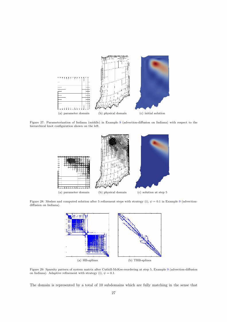
(a) parameter domain (b) physical domain (c) initial solution

Figure 27: Parameterization of Indiana (middle) in Example 9 (advection-diffusion on Indiana) with respect to thehierarchical knot configuration shown on the left.

(a) parameter domain (b) physical domain (c) solution at step 5

Figure 28: Meshes and computed solution after 5 refinement steps with strategy (i), ψ = 0.1 in Example 9 (advection-diffusion on Indiana).

(a) HB-splines (b) THB-splines

Figure 29: Sparsity pattern of system matrix after Cuthill-McKee-reordering at step 5, Example 9 (advection-diffusionon Indiana). Adaptive refinement with strategy (i), ψ = 0.1.

The domain is represented by a total of 10 subdomains which are fully matching in the sense that

27

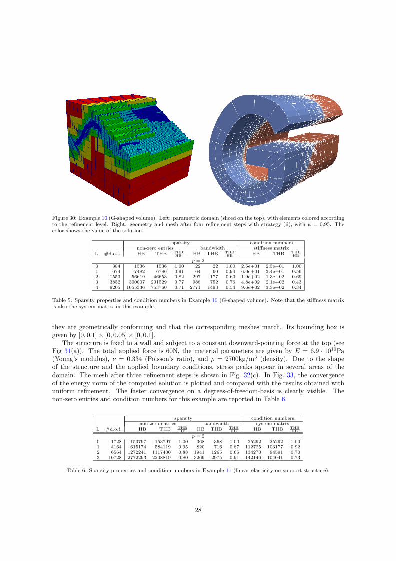
Figure 30: Example 10 (G-shaped volume). Left: parametric domain (sliced on the top), with elements colored accordingto the refinenent level. Right: geometry and mesh after four refinement steps with strategy (ii), with ψ = 0.95. Thecolor shows the value of the solution.

sparsity condition numbersnon-zero entries bandwidth stiffness matrix


HB HB THB THBHB

p = 20 384 1536 1536 1.00 22 22 1.00 2.5e+01 2.5e+01 1.001 674 7482 6786 0.91 64 60 0.94 6.0e+01 3.4e+01 0.562 1553 56619 46653 0.82 297 177 0.60 1.9e+02 1.3e+02 0.693 3852 300007 231529 0.77 988 752 0.76 4.8e+02 2.1e+02 0.434 9205 1055336 753760 0.71 2771 1493 0.54 9.6e+02 3.3e+02 0.34

Table 5: Sparsity properties and condition numbers in Example 10 (G-shaped volume). Note that the stiffness matrixis also the system matrix in this example.

they are geometrically conforming and that the corresponding meshes match. Its bounding box isgiven by [0, 0.1]× [0, 0.05]× [0, 0.1].

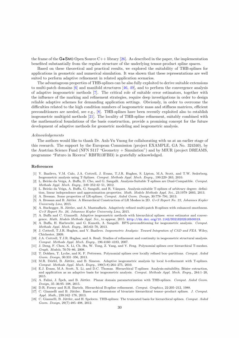
The structure is fixed to a wall and subject to a constant downward-pointing force at the top (seeFig 31(a)). The total applied force is 60N, the material parameters are given by E = 6.9 · 1010Pa(Young’s modulus), ν = 0.334 (Poisson’s ratio), and ρ = 2700kg/m3 (density). Due to the shapeof the structure and the applied boundary conditions, stress peaks appear in several areas of thedomain. The mesh after three refinement steps is shown in Fig. 32(c). In Fig. 33, the convergenceof the energy norm of the computed solution is plotted and compared with the results obtained withuniform refinement. The faster convergence on a degrees-of-freedom-basis is clearly visible. Thenon-zero entries and condition numbers for this example are reported in Table 6.

sparsity condition numbersnon-zero entries bandwidth system matrix


HB HB THB THBHB

p = 20 1728 153797 153797 1.00 368 368 1.00 25292 25292 1.001 4164 615174 584119 0.95 820 716 0.87 112725 103177 0.922 6564 1272241 1117400 0.88 1941 1265 0.65 134270 94591 0.703 10728 2772293 2208819 0.80 3269 2975 0.91 142146 104041 0.73

Table 6: Sparsity properties and condition numbers in Example 11 (linear elasticity on support structure).

28

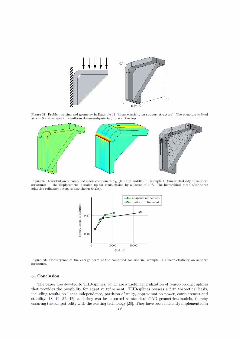
Figure 31: Problem setting and geometry in Example 11 (linear elasticity on support structure). The structure is fixedat x = 0 and subject to a uniform downward-pointing force at the top.

Figure 32: Distribution of computed stress component σ22 (left and middle) in Example 11 (linear elasticity on supportstructure) — the displacement is scaled up for visualization by a factor of 104. The hierarchical mesh after threeadaptive refinement steps is also shown (right).

0 10000 20000

0.16

0.17

# d.o.f.

energ

ynorm

of

solu

tion

adaptive refinement

uniform refinement

Figure 33: Convergence of the energy norm of the computed solution in Example 11 (linear elasticity on supportstructure).

5. Conclusion

The paper was devoted to THB-splines, which are a useful generalization of tensor-product splinesthat provides the possibility for adaptive refinement. THB-splines possess a firm theoretical basis,including results on linear independence, partition of unity, approximation power, completeness andstability [18, 19, 32, 42], and they can be exported as standard CAD geometries/models, therebyensuring the compatibility with the existing technology [28]. They have been efficiently implemented in

29

the frame of the G+++SMO Open Source C++ library [26]. As described in the paper, the implementationbenefited substantially from the regular structure of the underlying tensor-product spline spaces.

Based on these theoretical and practical results, we explored the suitability of THB-splines forapplications in geometric and numerical simulation. It was shown that these representations are wellsuited to perform adaptive refinement in related application scenarios.

The advantageous properties of THB-splines can be also fully exploited to derive suitable extensionsto multi-patch domains [6] and manifold structures [46, 49], and to perform the convergence analysisof adaptive isogeometric methods [7]. The critical role of suitable error estimators, together withthe influence of the marking and refinement strategies, require deep investigations in order to designreliable adaptive schemes for demanding application settings. Obviously, in order to overcome thedifficulties related to the high condition numbers of isogeometric mass and stiffness matrices, efficientpreconditioners are needed, see e.g., [8]. THB-splines have been recently exploited also to establishisogeometric multigrid methods [21]. The locality of THB-spline refinement, suitably combined withthe mathematical foundations of the basis construction, provide a promising concept for the futuredevelopment of adaptive methods for geometric modeling and isogeometric analysis.

Acknowledgements

The authors would like to thank Dr. Anh-Vu Vuong for collaborating with us at an earlier stage ofthis research. The support by the European Commission (project EXAMPLE, GA No. 324340), bythe Austrian Science Fund (NFN S117 “Geometry + Simulation”) and by MIUR (project DREAMS,programme “Futuro in Ricerca” RBFR13FBI3) is gratefully acknowledged.

References

[1] Y. Bazilevs, V.M. Calo, J.A. Cottrell, J. Evans, T.J.R. Hughes, S. Lipton, M.A. Scott, and T.W. Sederberg.Isogeometric analysis using T-Splines. Comput. Methods Appl. Mech. Engrg., 199:229–263, 2010.

[2] L. Beirao da Veiga, A. Buffa, D. Cho, and G. Sangalli. Analysis-Suitable T-splines are Dual-Compatible. Comput.Methods Appl. Mech. Engrg., 249–252:42–51, 2012.

[3] L. Beirao da Veiga, A. Buffa, G. Sangalli, and R. Vazquez. Analysis-suitable T-splines of arbitrary degree: defini-tion, linear independence and approximation properties. Math. Models Methods Appl. Sci., 23:1979–2003, 2013.

[4] A. Bressan. Some properties of LR-splines. Comput. Aided Geom. Design, 30:778–794, 2013.[5] A. Bressan and B. Juttler. A Hierarchical Construction of LR Meshes in 2D. G+S Report No. 23, Johannes Kepler

University Linz, 2015.[6] A. Buchegger, B. Juttler, and A. Mantzaflaris. Adaptively refined multi-patch B-splines with enhanced smothness.

G+S Report No. 26, Johannes Kepler University Linz, 2015.[7] A. Buffa and C. Giannelli. Adaptive isogeometric methods with hierarchical splines: error estimator and conver-

gence. Math. Models Methods Appl. Sci., to appear, 2015. http://dx.doi.org/10.1142/S0218202516500019.[8] A. Buffa, H. Harbrecht, and G. Kunoth, A. Sangalli. BPX-preconditioning for isogeometric analysis. Comput.

Methods Appl. Mech. Engrg., 265:63–70, 2013.[9] J. Cottrell, T.J.R. Hughes, and Y. Bazilevs. Isogeometric Analysis: Toward Integration of CAD and FEA. Wiley,

Chichester, 2009.[10] J.A. Cottrell, T.J.R. Hughes, and A. Reali. Studies of refinement and continuity in isogeometric structural analysis.

Comput. Methods Appl. Mech. Engrg., 196:4160–4183, 2007.[11] J. Deng, F. Chen, X. Li, Ch. Hu, W. Tong, Z. Yang, and Y. Feng. Polynomial splines over hierarchical T-meshes.

Graph. Models, 70:76–86, 2008.[12] T. Dokken, T. Lyche, and K. F. Pettersen. Polynomial splines over locally refined box–partitions. Comput. Aided

Geom. Design, 30:331–356, 2013.[13] M.R. Dorfel, B. Juttler, and B. Simeon. Adaptive isogeometric analysis by local h-refinement with T-splines.

Comput. Methods Appl. Mech. Engrg., 199(5-8):264–275, 2010.[14] E.J. Evans, M.A. Scott, X. Li, and D.C. Thomas. Hierarchical T-splines: Analysis-suitability, Bezier extraction,

and application as an adaptive basis for isogeometric analysis. Comput. Methods Appl. Mech. Engrg., 284:1–20,2015.

[15] A. Falini, J. Speh, and B. Juttler. Planar domain parameterization with THB-splines. Comput. Aided Geom.Design, 35–36:95–108, 2015.

[16] D.R. Forsey and R.H. Bartels. Hierarchical B-spline refinement. Comput. Graphics, 22:205–212, 1988.[17] C. Giannelli and B. Juttler. Bases and dimensions of bivariate hierarchical tensor–product splines. J. Comput.

Appl. Math., 239:162–178, 2013.[18] C. Giannelli, B. Juttler, and H. Speleers. THB-splines: The truncated basis for hierarchical splines. Comput. Aided

Geom. Design, 29(7):485–498, 2012.

30

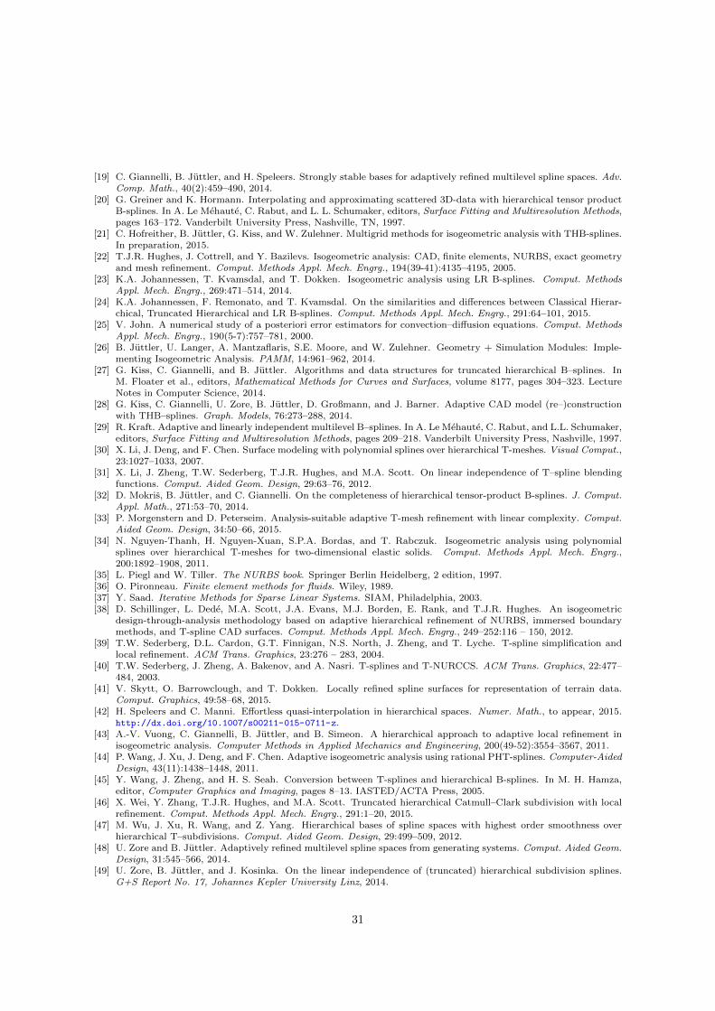
http://dx.doi.org/10.1142/S0218202516500019

[19] C. Giannelli, B. Juttler, and H. Speleers. Strongly stable bases for adaptively refined multilevel spline spaces. Adv.Comp. Math., 40(2):459–490, 2014.

[20] G. Greiner and K. Hormann. Interpolating and approximating scattered 3D-data with hierarchical tensor productB-splines. In A. Le Mehaute, C. Rabut, and L. L. Schumaker, editors, Surface Fitting and Multiresolution Methods,pages 163–172. Vanderbilt University Press, Nashville, TN, 1997.

[21] C. Hofreither, B. Juttler, G. Kiss, and W. Zulehner. Multigrid methods for isogeometric analysis with THB-splines.In preparation, 2015.

[22] T.J.R. Hughes, J. Cottrell, and Y. Bazilevs. Isogeometric analysis: CAD, finite elements, NURBS, exact geometryand mesh refinement. Comput. Methods Appl. Mech. Engrg., 194(39-41):4135–4195, 2005.

[23] K.A. Johannessen, T. Kvamsdal, and T. Dokken. Isogeometric analysis using LR B-splines. Comput. MethodsAppl. Mech. Engrg., 269:471–514, 2014.

[24] K.A. Johannessen, F. Remonato, and T. Kvamsdal. On the similarities and differences between Classical Hierar-chical, Truncated Hierarchical and LR B-splines. Comput. Methods Appl. Mech. Engrg., 291:64–101, 2015.

[25] V. John. A numerical study of a posteriori error estimators for convection–diffusion equations. Comput. MethodsAppl. Mech. Engrg., 190(5-7):757–781, 2000.

[26] B. Juttler, U. Langer, A. Mantzaflaris, S.E. Moore, and W. Zulehner. Geometry + Simulation Modules: Imple-menting Isogeometric Analysis. PAMM, 14:961–962, 2014.

[27] G. Kiss, C. Giannelli, and B. Juttler. Algorithms and data structures for truncated hierarchical B–splines. InM. Floater et al., editors, Mathematical Methods for Curves and Surfaces, volume 8177, pages 304–323. LectureNotes in Computer Science, 2014.

[28] G. Kiss, C. Giannelli, U. Zore, B. Juttler, D. Großmann, and J. Barner. Adaptive CAD model (re–)constructionwith THB–splines. Graph. Models, 76:273–288, 2014.

[29] R. Kraft. Adaptive and linearly independent multilevel B–splines. In A. Le Mehaute, C. Rabut, and L.L. Schumaker,editors, Surface Fitting and Multiresolution Methods, pages 209–218. Vanderbilt University Press, Nashville, 1997.

[30] X. Li, J. Deng, and F. Chen. Surface modeling with polynomial splines over hierarchical T-meshes. Visual Comput.,23:1027–1033, 2007.

[31] X. Li, J. Zheng, T.W. Sederberg, T.J.R. Hughes, and M.A. Scott. On linear independence of T–spline blendingfunctions. Comput. Aided Geom. Design, 29:63–76, 2012.

[32] D. Mokris, B. Juttler, and C. Giannelli. On the completeness of hierarchical tensor-product B-splines. J. Comput.Appl. Math., 271:53–70, 2014.

[33] P. Morgenstern and D. Peterseim. Analysis-suitable adaptive T-mesh refinement with linear complexity. Comput.Aided Geom. Design, 34:50–66, 2015.

[34] N. Nguyen-Thanh, H. Nguyen-Xuan, S.P.A. Bordas, and T. Rabczuk. Isogeometric analysis using polynomialsplines over hierarchical T-meshes for two-dimensional elastic solids. Comput. Methods Appl. Mech. Engrg.,200:1892–1908, 2011.

[35] L. Piegl and W. Tiller. The NURBS book. Springer Berlin Heidelberg, 2 edition, 1997.[36] O. Pironneau. Finite element methods for fluids. Wiley, 1989.[37] Y. Saad. Iterative Methods for Sparse Linear Systems. SIAM, Philadelphia, 2003.[38] D. Schillinger, L. Dede, M.A. Scott, J.A. Evans, M.J. Borden, E. Rank, and T.J.R. Hughes. An isogeometric

design-through-analysis methodology based on adaptive hierarchical refinement of NURBS, immersed boundarymethods, and T-spline CAD surfaces. Comput. Methods Appl. Mech. Engrg., 249–252:116 – 150, 2012.

[39] T.W. Sederberg, D.L. Cardon, G.T. Finnigan, N.S. North, J. Zheng, and T. Lyche. T-spline simplification andlocal refinement. ACM Trans. Graphics, 23:276 – 283, 2004.

[40] T.W. Sederberg, J. Zheng, A. Bakenov, and A. Nasri. T-splines and T-NURCCS. ACM Trans. Graphics, 22:477–484, 2003.

[41] V. Skytt, O. Barrowclough, and T. Dokken. Locally refined spline surfaces for representation of terrain data.Comput. Graphics, 49:58–68, 2015.

[42] H. Speleers and C. Manni. Effortless quasi-interpolation in hierarchical spaces. Numer. Math., to appear, 2015.http://dx.doi.org/10.1007/s00211-015-0711-z.

[43] A.-V. Vuong, C. Giannelli, B. Juttler, and B. Simeon. A hierarchical approach to adaptive local refinement inisogeometric analysis. Computer Methods in Applied Mechanics and Engineering, 200(49-52):3554–3567, 2011.

[44] P. Wang, J. Xu, J. Deng, and F. Chen. Adaptive isogeometric analysis using rational PHT-splines. Computer-AidedDesign, 43(11):1438–1448, 2011.

[45] Y. Wang, J. Zheng, and H. S. Seah. Conversion between T-splines and hierarchical B-splines. In M. H. Hamza,editor, Computer Graphics and Imaging, pages 8–13. IASTED/ACTA Press, 2005.

[46] X. Wei, Y. Zhang, T.J.R. Hughes, and M.A. Scott. Truncated hierarchical Catmull–Clark subdivision with localrefinement. Comput. Methods Appl. Mech. Engrg., 291:1–20, 2015.

[47] M. Wu, J. Xu, R. Wang, and Z. Yang. Hierarchical bases of spline spaces with highest order smoothness overhierarchical T–subdivisions. Comput. Aided Geom. Design, 29:499–509, 2012.

[48] U. Zore and B. Juttler. Adaptively refined multilevel spline spaces from generating systems. Comput. Aided Geom.Design, 31:545–566, 2014.

[49] U. Zore, B. Juttler, and J. Kosinka. On the linear independence of (truncated) hierarchical subdivision splines.G+S Report No. 17, Johannes Kepler University Linz, 2014.

31

http://dx.doi.org/10.1007/s00211-015-0711-z

THB-splines: An effective mathematical technology for ...

Documents

Transcript of THB-splines: An effective mathematical technology for ...