Textures and Majorana Excitations in Multi...
114
Textures and Majorana Excitations in Multi-Component Neutral Fermi Superfluids 2011, March YASUMASA TSUTSUMI Graduate School of Natural Science and Technology (Doctor’s Course) OKAYAMA UNIVERSITY
Transcript of Textures and Majorana Excitations in Multi...

Textures and Majorana Excitations
in Multi-Component
Neutral Fermi Superfluids
2011, March
YASUMASA TSUTSUMI
Graduate School of Natural Science and Technology
(Doctor’s Course)
OKAYAMA UNIVERSITY

Abstract
Textures and Majorana excitations in multi-component neutral Fermi superfluids of 3Heatoms and atomic gases are investigated. The superfluid 3He consists of p-wave Cooperpairs without doubt. Since the interaction of atomic gases can be tuned by the Feshbachresonance, superfluids of Fermi atomic gases through a p-wave scattering will be realizedin the near future. Such p-wave superfluids construct a spatial structure of the superfluidorder parameter (OP), i.e. texture, by vortices or boundary conditions to lower free energyusing the multi-component OP thoroughly. Fermi superfluids have low energy excitations atvortices and boundaries, where a superfluid gap is suppressed. Certain excitations in p-waveFermi superfluids behave as Majorana quasi-particles (QPs) or Majorana fermions. Existenceof the Majorana excitations at vortices and boundary in p-wave Fermi superfluids reflectsthat p-wave superfluids can be regarded as topological superfluids. Textures and Majoranaexcitations in the superfluid 3He and superfluids of p-wave atomic gases are discussed inconnection with realistic experiments.
First, recent experiments for the textures of the superfluid 3He A-phase confined in anarrow cylinder are discussed. Compered to the experiments, the radial disgyration, Mermin-Ho texture, and Pan-Am texture are calculated by the Ginzburg-Landau (GL) theory. Theradial disgyration is stable at rest for the cylinders by using the experiments, and the Mermin-Ho texture is stable under rotation. The results show good agreement with the experimentalresults.
Features of the Majorana excitations are different for a chiral superfluid and helical su-perfluid, which are different in the topological nature. In the superfluid 3He, the chiralsuperfluid is realized in the A-phase and the helical superfluid is realized in the B-phase.Then, we calculate the Majorana edge state for the superfluid 3He in a realistic slab usingthe quasi-classical theory. For the A-phase, dispersion relation of the QPs at the edge con-structs a Dirac valley. For the B-phase, dispersion relation of the QPs at the edge constructsa Majorana cone. The Majorana QPs exist both phases. Based on a result, we suggestexperiments to observe the Majorana QPs.
Finally, textures for superfluids of p-wave atomic gases are calculated by the GL theory.The textures are different from the superfluid 3He by the boundary condition, because Fermiatomic gases are confined in harmonic trap potential by a magnetic field. In quasi-two dimen-sional trap potential, conditions to stabilize a quantized vortex with Majorana QP for trapfrequency and rotation frequency are derived. This work is helpful to confirm superfluidityand apply the system to a topological quantum computer when superfluids of p-wave Fermiatomic gases are realized in the future.
i

Acknowledgments
I would like to express my gratitude to Professor Kazushige Machida whose comments andsuggestions were of inestimable value for my study. He has guided me to accomplishment ofmy research by proper advice and prepared environment in which I can concentrate on myinvestigation.
I would like to thank Professor Masanori Ichioka for invaluable comments and provid-ing the fundamental computer program for solving the Eilenberger equation and Ginzburg-Landau equation which formed the basis of my research. I would also like to thank ProfessorTakeshi Mizushima for helpful discussions. In particular, I can understand Majorana excita-tions by his instruction.
I am indebted to Dr. Ken Izumina, Professor Ryosuke Ishiguro, Professor Minoru Kubota,Professor Osamu Ishikawa, Professor Yutaka Sasaki, and Professor Takeo Takagi for helpfuldiscussions about the experiments in ISSP, Univ. of Tokyo. I am also indebted to ProfessorTetsuo Ohmi for helpful discussions about the superfluid 3He.
I want to thank everyone in the Mathematical Physics Laboratory for advice about re-search and life.
Finally, I would like to acknowledge the financial support of the Research Fellowships ofthe Japan Society for the Promotion of Science for Young Scientists.
iii


Contents
1 Introduction 11.1 Background . . . . . . . . . . . . . . . . . . . . . . . . . . . . . . . . . . . . . 11.2 Outline of this thesis . . . . . . . . . . . . . . . . . . . . . . . . . . . . . . . . 1
2 Formulation of superfluidity 32.1 Bogoliubov-de Gennes theory . . . . . . . . . . . . . . . . . . . . . . . . . . . 52.2 Gor’kov theory . . . . . . . . . . . . . . . . . . . . . . . . . . . . . . . . . . . 52.3 Quasi-classical theory . . . . . . . . . . . . . . . . . . . . . . . . . . . . . . . 7
2.3.1 Eilenberger equation . . . . . . . . . . . . . . . . . . . . . . . . . . . . 72.3.2 Riccati equations . . . . . . . . . . . . . . . . . . . . . . . . . . . . . . 8
2.4 Ginzburg-Landau theory . . . . . . . . . . . . . . . . . . . . . . . . . . . . . . 9
3 Multi-component neutral Fermi superfluids 113.1 Superfluid 3He . . . . . . . . . . . . . . . . . . . . . . . . . . . . . . . . . . . 11
3.1.1 Texture . . . . . . . . . . . . . . . . . . . . . . . . . . . . . . . . . . . 133.1.2 Half-quantum vortex . . . . . . . . . . . . . . . . . . . . . . . . . . . . 13
3.2 Fermi atomic gases . . . . . . . . . . . . . . . . . . . . . . . . . . . . . . . . . 143.2.1 Feshbach resonance . . . . . . . . . . . . . . . . . . . . . . . . . . . . . 153.2.2 p-wave resonant Fermi atomic gases . . . . . . . . . . . . . . . . . . . 16
4 Majorana excitations 194.1 Majorana quasi-particle in vortex . . . . . . . . . . . . . . . . . . . . . . . . . 19
4.1.1 Non-Abelian statistics . . . . . . . . . . . . . . . . . . . . . . . . . . . 234.2 Majorana edge fermion . . . . . . . . . . . . . . . . . . . . . . . . . . . . . . . 24
4.2.1 Chiral edge state . . . . . . . . . . . . . . . . . . . . . . . . . . . . . . 244.2.2 Helical edge state . . . . . . . . . . . . . . . . . . . . . . . . . . . . . . 25
5 Superfluid 3He in a cylinder 295.1 Formulation . . . . . . . . . . . . . . . . . . . . . . . . . . . . . . . . . . . . . 31
5.1.1 Ginzburg-Landau functional for the superfluid 3He . . . . . . . . . . . 315.1.2 Numerics and boundary condition . . . . . . . . . . . . . . . . . . . . 33
5.2 Stable textures . . . . . . . . . . . . . . . . . . . . . . . . . . . . . . . . . . . 345.2.1 Radial disgyration (RD) . . . . . . . . . . . . . . . . . . . . . . . . . . 345.2.2 Mermin-Ho (MH) . . . . . . . . . . . . . . . . . . . . . . . . . . . . . 375.2.3 Pan-Am texture . . . . . . . . . . . . . . . . . . . . . . . . . . . . . . 37
5.3 Size-dependence and magnetic field effects . . . . . . . . . . . . . . . . . . . . 405.3.1 Size-dependence and the critical rotation speed . . . . . . . . . . . . . 405.3.2 Magnetic field effect . . . . . . . . . . . . . . . . . . . . . . . . . . . . 41
v

vi CONTENTS
5.4 Analysis of experiments . . . . . . . . . . . . . . . . . . . . . . . . . . . . . . 435.4.1 R=50 µm . . . . . . . . . . . . . . . . . . . . . . . . . . . . . . . . . . 435.4.2 R=115 µm . . . . . . . . . . . . . . . . . . . . . . . . . . . . . . . . . 44
5.5 Summary . . . . . . . . . . . . . . . . . . . . . . . . . . . . . . . . . . . . . . 45
6 Superfluid 3He in a slab 476.1 Quasi-classical theory and order parameter . . . . . . . . . . . . . . . . . . . 486.2 System geometry and numerical methods . . . . . . . . . . . . . . . . . . . . 506.3 A-phase . . . . . . . . . . . . . . . . . . . . . . . . . . . . . . . . . . . . . . . 51
6.3.1 D = 8ξ0: Thin slab for A-phase . . . . . . . . . . . . . . . . . . . . . . 526.3.2 D = 14ξ0: Thick slab for A-phase . . . . . . . . . . . . . . . . . . . . . 54
6.4 B-phase . . . . . . . . . . . . . . . . . . . . . . . . . . . . . . . . . . . . . . . 566.4.1 D = 30ξ0: Thick slab for B-phase . . . . . . . . . . . . . . . . . . . . . 576.4.2 D = 14ξ0: Thin slab for B-phase . . . . . . . . . . . . . . . . . . . . . 596.4.3 Dependence of the energy splitting on the thickness . . . . . . . . . . 60
6.5 Discussion . . . . . . . . . . . . . . . . . . . . . . . . . . . . . . . . . . . . . . 616.5.1 Majorana zero modes in the A- and B-phases . . . . . . . . . . . . . . 616.5.2 Stripe phase . . . . . . . . . . . . . . . . . . . . . . . . . . . . . . . . . 616.5.3 Experimental proposal . . . . . . . . . . . . . . . . . . . . . . . . . . . 62
6.6 Summary . . . . . . . . . . . . . . . . . . . . . . . . . . . . . . . . . . . . . . 63
7 p-wave resonant superfluids of Fermi atomic gases 657.1 Formulation . . . . . . . . . . . . . . . . . . . . . . . . . . . . . . . . . . . . . 667.2 Preliminary considerations . . . . . . . . . . . . . . . . . . . . . . . . . . . . . 687.3 Cigar shape trap . . . . . . . . . . . . . . . . . . . . . . . . . . . . . . . . . . 69
7.3.1 Stable texture at rest . . . . . . . . . . . . . . . . . . . . . . . . . . . 697.3.2 Half-quantum vortex under rotation . . . . . . . . . . . . . . . . . . . 71
7.4 Pancake shape trap . . . . . . . . . . . . . . . . . . . . . . . . . . . . . . . . . 737.4.1 Axis symmetric texture at rest . . . . . . . . . . . . . . . . . . . . . . 737.4.2 Vortices under rotation . . . . . . . . . . . . . . . . . . . . . . . . . . 75
7.5 Quasi-2D trap . . . . . . . . . . . . . . . . . . . . . . . . . . . . . . . . . . . . 757.5.1 Possible types of axisymmetric structure and a vortex . . . . . . . . . 787.5.2 Stability region of the singular vortex . . . . . . . . . . . . . . . . . . 79
7.6 Summary . . . . . . . . . . . . . . . . . . . . . . . . . . . . . . . . . . . . . . 84
8 Conclusion 878.1 Summary of this thesis . . . . . . . . . . . . . . . . . . . . . . . . . . . . . . . 878.2 Future studies . . . . . . . . . . . . . . . . . . . . . . . . . . . . . . . . . . . . 88
A Symmetry of quasi-classical Green’s function 89
B Angular momentum of the A-phase in a slab 91B.1 Angular momentum by Matsubara Green’s function . . . . . . . . . . . . . . 92B.2 Angular momentum by retarded Green’s function . . . . . . . . . . . . . . . . 93
C Ginzburg-Landau functional under rotation 97
D Bulk energy in Ginzburg-Landau functional 99

Chapter 1
Introduction
1.1 Background
Superconductivity was discovered by Kamerlingh Onnes in 1911. After decades, phenomeno-logical Ginzburg-Landau (GL) theory and microscopic Bardeen-Cooper-Schrieffer (BCS) the-ory give a fundamental understanding of the conventional superconductivity.
In neutral Fermi systems, the first superfluid phase was discovered in the liquid 3He byOsheroff et al. [1] The superfluid 3He is unconventional in which Cooper pairs have the spin-triplet p-wave symmetry [2]. This understanding progressed by generalization of the BCStheory. The GL theory gives understanding of textures (spatial structures of superfluid orderparameter) and exotic vortices (e.g. a half-quantum vortex). However, since the experimentof the superfluid 3He is required low temperature of the order of mK, various assignmentshave remained yet. Moreover, the superfluid 3He is one of the candidate systems in whichMajorana quasi-particles (QPs) and fermions live. They are discussed also in the condensedmatter physics recently [3].
Another progress of neutral Fermi superfluidity is in ultra-cold Fermi atomic gases [4].In 1995, Bose-Einstein condensates (BECs) were realized for Bose atomic gases [5, 6, 7].After about 10 years, BECs by molecules of Fermi atoms were observed [8, 9, 10]. Shortlyafter then, superfluids by Cooper pairs of Fermi atoms were also observed [11, 12]. Recently,molecules of Fermi atoms through a p-wave scattering can be create [13, 14, 15, 16, 17, 18].In the near future, BECs by p-wave molecules and superfluids by Cooper pairs with p-waveinteraction are expected. The superfluids of p-wave Fermi atomic gases involve textures,exotic vortices, and Majorana QPs and fermions. The Fermi atomic gases have the advantageof maneuverability than the superfluid 3He.
1.2 Outline of this thesis
In this thesis, p-wave superfluids of neutral Fermi systems are discussed theoretically. Thisthesis has two main subjects which are textures and Majorana excitations. p-wave super-fluids construct a texture by vortices or boundary conditions to lower free energy using themulti-component superfluid order parameter (OP) thoroughly. Fermi superfluids have lowenergy excitations at vortices and boundaries, where a superfluid gap is suppressed. Certainexcitations in p-wave Fermi superfluids behave as Majorana QPs or Majorana fermions. Theyare discussed in connection with realistic experiments.
The general formulation of superfluidity within the mean-field theory is discussed in
1

2 CHAPTER 1. INTRODUCTION
Chap. 2. Starting from the BCS Hamiltonian, the Bogoliubov-de Gennes (BdG) equationis derived by the unitary transformation. By the BdG equation, we can demonstrate thatcertain low energy excitations in p-wave superfluids behaves as Majorana QPs or Majoranafermions. Another way from the BCS Hamiltonian is to derive the Gor’kov equation usingGreen’s function. By quasi-classical approximation of the Gor’kov equation, we derive theEilenberger equation and Riccati equations with quasi-classical Green’s function. The Eilen-berger equation and Riccati equations are used for the calculation of the QP state in Chap. 6.In the vicinity of the superfluid transition temperature, the Ginzburg-Landau (GL) theoryis derived from the symmetric consideration. The GL theory is used for the discussion oftextures in Chaps. 5 and 7.
In Chap. 3, we introduce the superfluid 3He and the superfluid of p-wave resonant Fermiatomic gases, which are multi-component neutral Fermi superfluids. The superfluid 3He istypical matter of p-wave neutral Fermi superfluids. Textures and a half-quantum vortex inthe superfluid 3He are also introduced in this chapter. The superfluid of p-wave resonantFermi atomic gases using Feshbach resonances are expected in the near future.
Majorana QPs and Majorana fermions are introduced in Chap. 4. A zero energy excitationat a vortex with an odd integer winding number behaves as a Majorana QP in p-wavesuperfluids. The Majorana QPs obey non-Abelian statistics, so that they can be utilizedfor a topological quantum computer. The Andreev bound states at the edge of p-wavesuperfluids are described by field operators of the Majorana fermions. There are two kindsof edge state: The chiral edge state appears in the superfluid 3He A-phase, and the helicaledge state appears in the B-phase.
In Chap. 5, our theoretical results are compared to recent experiments for the texturesof the superfluid 3He A-phase confined in a narrow cylinder [19, 20]. Textures consist of fewvortices can be observed because the rotating cryostat in ISSP, Univ. of Tokyo achieves highrotation speed. Compered to the experiments, the radial disgyration, Mermin-Ho texture,and Pan-Am texture are calculated by the GL theory. The radial disgyration is stable atrest for the cylinders by using the experiments, and the Mermin-Ho texture is stable underrotation. The results show good agreement with the experimental results.
We calculate the Majorana edge state for the superfluid 3He in a realistic slab using thequasi-classical theory [21, 22, 23] in Chap. 6. For the A-phase, dispersion relation of the QPsat the edge constructs a Dirac valley. For the B-phase, dispersion relation of the QPs at theedge constructs a Majorana cone. The Majorana QPs exist both phases. Based on a result,we suggest experiments to observe the Majorana QPs.
In Chap. 7, textures for superfluids of p-wave atomic gases are calculated by the GLtheory [24, 25]. The textures are different from the superfluid 3He by the boundary condition,because Fermi atomic gases are confined in harmonic trap potential. In quasi-two dimensionaltrap potential, there is a vortex with Majorana QP [26]. This work is helpful when superfluidsof p-wave Fermi atomic gases are realized in the future.
The final chapter devotes for a summary of this thesis and a view for future studies.

Chapter 2
Formulation of superfluidity
The Bardeen-Cooper-Schrieffer (BCS) Hamiltonian with fermion field operators ψα(r) in theSchrodinger picture is
HBCS =∑αβ
∫d3r1d
3r2
[ψ†
α(r1)Kαβ(r1, r2)ψβ(r2)
+12
∑δγ
V γ,δα,β (r12)ψ†
α(r1)ψ†β(r2)ψγ(r2)ψδ(r1)
], (2.1)
where
Kαβ(r1, r2) ≡ δαβδ(r1 − r2)[−~2∇2
2m− µ
]+ Σαβ(r1, r2), (2.2)
includes kinetic term, chemical potential µ, and self-energy Σαβ(r1, r2). If the interactionV γ,δ
α,β (r12) is invariant under rotation in the spin space,
V γ,δα,β (r12) = V1(r12)δαδδβγ + V2(r12)σαδ · σβγ , (2.3)
where σ is the Pauli matrix in the spin-1/2 space and r12 ≡ |r1 − r2|. Here, we define theorder parameter (OP) of the superfluid state as
∆αβ(r1, r2) ≡∑γδ
V γ,δα,β (r12) 〈ψγ(r2)ψδ(r1)〉 ,
∆∗αβ(r1, r2) ≡
∑γδ
V β,αδ,γ (r12)
⟨ψ†
δ(r1)ψ†γ(r2)
⟩,
(2.4)
where 〈· · · 〉 denotes statistical average. The statistical average of field operators is decom-posed into the orbital and spin parts: 〈ψγ(r2)ψδ(r1)〉 ≡ χ(r1, r2)φ(γ, δ). Then, the spinfunction satisfies
∑γδ σαδ · σβγφ(γ, δ) = −3φ(β, α) for the spin-singlet state and
∑γδ σαδ ·
σβγφ(γ, δ) = φ(β, α) for the spin-triplet state. Hence, we find∑γδ
V γ,δα,βφ(γ, δ) = [V1(r12) + λV2(r12)]φ(β, α) ≡ V (r12)φ(β, α), (2.5)
3
4 CHAPTER 2. FORMULATION OF SUPERFLUIDITY
where λ = −3 for the spin-singlet state and λ = 1 for the spin-triplet state. Therefore, thedefinition of the OP can be rewritten as
∆αβ(r1, r2) ≡ V (r12) 〈ψβ(r2)ψα(r1)〉 ,
∆∗αβ(r1, r2) ≡ V (r12)
⟨ψ†
α(r1)ψ†β(r2)
⟩.
(2.6)
Here, we perform the mean-field approximation for the BCS Hamiltonian. The mean-fieldHamiltonian is described by
H =∑αβ
∫d3r1d
3r2
[ψ†
α(r1)Kαβ(r1, r2)ψβ(r2)
+12∆∗
αβ(r1, r2)ψβ(r2)ψα(r1) +12∆αβ(r1, r2)ψ†
α(r1)ψ†β(r2)
− 12
∆αβ(r1, r2)∆∗αβ(r1, r2)
V (r12)
], (2.7)
where the last term can be included in c-number E0.Here, we introduce the four dimensional Nambu spinor Ψ(r) and the 4×4 matrix K(r1, r2)
and ∆(r1, r2) as
Ψ(r) ≡[ψ↑(r), ψ↓(r), ψ†
↑(r), ψ†↓(r)
]T, (2.8)
K(r1, r2) ≡(K(r1, r2) 0
0 −KT (r2, r1)
),
K(r1, r2) ≡
δ(r1 − r2)[−∇2
2m − µ↑
]+ Σ↑↑(r1, r2) Σ↑↓(r1, r2)
Σ↓↑(r1, r2) δ(r1 − r2)[−∇2
2m − µ↓
]+ Σ↓↓(r1, r2)
,
(2.9)
∆(r1, r2) ≡(
0 ∆(r1, r2)∆†(r2, r1) 0
), ∆(r1, r2) ≡
(∆↑↑(r1, r2) ∆↑↓(r1, r2)∆↓↑(r1, r2) ∆↓↓(r1, r2)
), (2.10)
where the superscript T indicates transposed matrices and µ↑,↓ is chemical potential includinglocal self-energy Σ↑↑(r, r) or Σ↓↓(r, r). The OP yields the symmetry ∆(r2, r1) = ±∆(r1, r2),where the sign + is for the spin-singlet state and − is for the spin-triplet state. In thefollowing, the “ordinary hat” indicates the 2 × 2 matrix in spin space and the “wide hat”indicates the 4 × 4 matrix in Nambu and spin spaces. Using the spinor and matrices, themean-field Hamiltonian is rewritten as
H = E0 +12
∫d3r1d
3r2Ψ†(r1)[K(r1, r2) + ∆(r1, r2)
]Ψ(r2). (2.11)
In this chapter, based on the mean-field Hamiltonian eq. (2.7) or eq. (2.11), we formulateequations described to the superfluid state. In Sec. 2.1, the Bogoliubov-de Gennes (BdG)equation is derived by the unitary transformation from eq. (2.11). The BdG equation ishelpful to understand Majorana excitations. In Sec. 2.2, we obtain the Gor’kov equations with
2.1. BOGOLIUBOV-DE GENNES THEORY 5
Green’s function from eq. (2.7). By quasi-classical approximation of the Gor’kov equations,we obtain the Eilenberger equation with quasi-classical Green’s function in Sec. 2.3. Fromthe Eilenberger equation, we obtain the Riccati equations which are convenient for analyticaland numerical calculation. In Sec. 2.4, we obtain the Ginzburg-Landau (GL) free energyfunctional from the symmetric consideration. The GL free energy functional is also obtainedfrom the microscopic theory. The quasi-classical theory and GL theory give main results inthis thesis.
2.1 Bogoliubov-de Gennes theory
We introduce the unitary transformation, so-called the Bogoliubov transformation, whichtransforms the spinor Ψ(r) to the basis composed of the quasi-particle (QP) operator γν :
Ψ(r) =∑
ν
uν(r)γν , γν ≡[γν,↑, γν,↓, γ
†ν,↑, γ
†ν,↓
]T, (2.12)
where the QP operator γν satisfies the fermion commutation relations,γν,α, γ
†µ,β
= δαβδνµ, γν,α, γµ,β =
γ†ν,α, γ
†µ,β
= 0. (2.13)
The unitary 4 × 4 matrix uν(r) must fulfill the orthonormal and completeness conditions,∫d3ru†ν(r)uµ(r) = δνµσ0, (2.14)
∑ν
u†ν(r1)uν(r2) = δ(r1 − r2)σ0, (2.15)
where σ0 is the 4 × 4 unit matrix.Using the QP basis defined in eq. (2.12), we find that the mean-field Hamiltonian in
eq. (2.11) can be diagonalized as
H = E0 +12
∑ν
γ†νEνγν , Eν ≡ diag [Eν,↑, Eν,↓,−Eν,↑,−Eν,↓] , (2.16)
where diag[· · · ] indicates diagonal matrices. Then, the matrix uν must fulfill the Bogoliubov-de Gennes (BdG) equation:∫
d3r2
[K(r1, r2) + ∆(r1, r2)
]uν(r2) = uν(r1)Eν . (2.17)
2.2 Gor’kov theory
Thermal Green’s function is defined by
Gαβ(r1, r2) ≡(Gαβ(r1, r2) Fαβ(r1, r2)Fαβ(r1, r2) Gαβ(r1, r2)
)
≡
−⟨Tτ
[ψα(r1)ψ
†β(r2)
]⟩−⟨Tτ
[ψα(r1)ψβ(r2)
]⟩−⟨Tτ
[ψ†
α(r1)ψ†β(r2)
]⟩−⟨Tτ
[ψ†
α(r1)ψβ(r2)]⟩ , (2.18)

6 CHAPTER 2. FORMULATION OF SUPERFLUIDITY
where
ψα(r) = eHτ/~ψα(r)e−Hτ/~,
ψ†α(r) = eHτ/~ψ†
α(r)e−Hτ/~,(2.19)
are field operators in the Heisenberg picture and (r) indicates (r, τ). From eq. (2.7), theimaginary time-derivative of the field operators are
~∂
∂τ1ψα(r1) =
∑β
∫d3r2
[−Kαβ(r1, r2)ψβ(r2, τ1) − ∆αβ(r1, r2)ψ
†β(r2, τ1)
],
~∂
∂τ1ψ†
α(r1) =∑β
∫d3r2
[Kβα(r2, r1)ψ
†β(r2, τ1) − ∆∗
βα(r2, r1)ψβ(r2, τ1)].
(2.20)
Using eq. (2.20) we can calculate the imaginary time-derivative of the Green’s function. Theimaginary time-derivative of the Green’s function gives Gor’kov equations:∑
γ
∫d3r3
(−~ ∂
∂τ1δαγδ(r1 − r3) −Kαγ(r1, r3) −∆αγ(r1, r3)
−∆∗γα(r3, r1) −~ ∂
∂τ1δαγδ(r1 − r3) +Kγα(r3, r1)
)× Gγβ(r3τ1, r2τ2) = ~δαβδ(r1 − r2)σ0, (2.21)
∑γ
∫d3r3Gαγ(r1τ1, r3τ2)
×
(~ ∂
∂τ2δγβδ(r3 − r2) −Kγβ(r3, r2) −∆γβ(r3, r2)
−∆∗βγ(r2, r3) ~ ∂
∂τ2δγβδ(r3 − r2) +Kβγ(r2, r3)
)= ~δαβδ(r1 − r2)σ0, (2.22)
where the imaginary time-derivative ∂/∂τ2 operates the left side of the Green’s function.The Gor’kov equations are more convenient in the frequency representation. By Fourier
transformation,
Gαβ(r1τ1, r2τ2) =kBT
~∑
n
e−iωn(τ1−τ2)Gαβ(r1, r2, ωn), (2.23)
δ(τ1 − τ2) =kBT
~∑
n
e−iωn(τ1−τ2), (2.24)
where ωn = (2n + 1)πkBT/~ is the Matsubara frequency with integer n. The Gor’kovequations are rewritten as∑
γ
∫d3r3
(i~ωnδαγδ(r1 − r3) −Kαγ(r1, r3) −∆αγ(r1, r3)
−∆∗γα(r3, r1) i~ωnδαγδ(r1 − r3) +Kγα(r3, r1)
)× Gγβ(r3, r2, ωn) = ~δαβδ(r1 − r2)σ0, (2.25)
∑γ
∫d3r3Gαγ(r1, r3, ωn)
×(i~ωnδγβδ(r3 − r2) −Kγβ(r3, r2) −∆γβ(r3, r2)
−∆∗βγ(r2, r3) i~ωnδγβδ(r3 − r2) +Kβγ(r2, r3)
)= ~δαβδ(r1 − r2)σ0. (2.26)
2.3. QUASI-CLASSICAL THEORY 7
2.3 Quasi-classical theory
We introduce the center-of-mass coordinate R = (r1 + r2)/2 and the relative coordinater = r1 − r2. The Green’s function is rewritten as
Gαβ(r1, r2, ωn) =∫
d3k
(2π)3Gαβ(R,k, ωn)eik·r, (2.27)
where k is the relative momentum.The quasi-classical approximation is valid when ∆/EF 1, or ξkF 1, where ∆ is
superfluid gap, EF is the Fermi energy, ξ is superfluid coherence length, and kF is the Fermiwave number. The condition is satisfied for most superconductors and the superfluid 3He, inwhich ∆/EF ∼ 10−3, and even for high-Tc superconductors, in which ∆/EF ∼ 10−2. Underthe condition, the Green’s function has a peak with a width of ∆ at the Fermi surface. Then,k-dependence of the Green’s function can be integrated by the energy ξk = ~2k2/(2m) − µ,and the relative momentum in the other integrand can be replaced by the Fermi momentumkF . The unimportant rapid oscillating term exp(ikF · r) can be neglected, because we takethe limit r → 0 for calculation of physical quantities from the Green’s function. The quasi-classical Green’s function is defined in Nambu space by∫
dξkσzG(R,k, ωn) ≡ g(R,kF , ωn) ≡ −iπ
(g(R,kF , ωn) if(R,kF , ωn)
−if(R,kF , ωn) −g(R,kF , ωn)
). (2.28)
The quasi-classical Green’s function satisfies a normalization condition g2 = −π2σ0.
2.3.1 Eilenberger equation
Using the relation σ2z = σ0, the Gor’kov equations (2.25) and (2.26) are rewritten as
∑γ
∫d3r3
δαγδ(r1 − r3)
[i~ωnσz +
(~2∇2
3
2m+ µ
)σ0
]
+(−Σαγ(r1, r3) ∆αγ(r1, r3)−∆∗
γα(r3, r1) −Σγα(r3, r1)
)σzGγβ(r3, r2, ωn) = ~δαβδ(r1 − r2)σ0, (2.29)
∑γ
∫d3r3σzGαγ(r1, r3, ωn)
×δγβδ(r3 − r2)
[i~ωnσz +
(~2∇2
3
2m+ µ
)σ0
]+(−Σγβ(r3, r2) ∆γβ(r3, r2)−∆∗
βγ(r2, r3) −Σβγ(r2, r3)
)= ~δαβδ(r1 − r2)σ0. (2.30)
By subtracting eq. (2.30) from eq. (2.29),
~2
2m(∇2
1 −∇22
)σzGαβ(r1, r2, ωn) +
[i~ωnσz, σzGαβ(r1, r2, ωn)
]+∑
γ
∫d3r3
[(−Σαγ(r1, r3) ∆αγ(r1, r3)−∆∗
γα(r3, r1) −Σγα(r3, r1)
)σzGγβ(r3, r2, ωn)
− σzGαγ(r1, r3, ωn)(−Σγβ(r3, r2) ∆γβ(r3, r2)−∆∗
βγ(r2, r3) −Σβγ(r2, r3)
)]= 0. (2.31)
8 CHAPTER 2. FORMULATION OF SUPERFLUIDITY
The derivative operators can be rewritten by the center-of-mass coordinate and relativecoordinate: ∇1 = ∇R/2 +∇r and ∇2 = ∇R/2−∇r. By the derivations operate the Green’sfunction in the Fourier representation eq. (2.27),
~2
2m(∇2
1 −∇22
)σzGαβ(r1, r2, ωn) =
∫d3k
(2π)3i~v · ∇RσzGαβ(R,k, ωn)eik·r, (2.32)
where v = ~k/m. Therefore, eq. (2.31) is
i~v · ∇RσzGαβ(R,k, ωn) +[i~ωnσz, σzGαβ(R,k, ωn)
]+∑
γ
[(−Σαγ(R,k) −∆αγ(R,k)∆∗
γα(R,k) −Σγα(R,−k)
)σzGγβ(R,k, ωn)
− σzGαγ(R,k, ωn)(−Σγβ(R,k) −∆γβ(R,k)∆∗
βγ(R,k) −Σβγ(R,−k)
)]= 0. (2.33)
Here, we use the quasi-classical approximation, i.e. the Green’s function is integrated bythe energy ξk and the other relative momentum is replaced by the Fermi momentum kF .Then, we obtain the Eilenberger equation with the quasi-classical Green’s function [27]:
i~vF · ∇Rg(R,kF , ωn) +[i~ωnσz − ∆(R,kF ) − Σ(R,kF ), g(R,kF , ωn)
]= 0, (2.34)
where vF is the Fermi velocity. The matrices are defined
∆(R,kF ) ≡(
0 ∆(R,kF )−∆†(R,kF ) 0
), Σ(R,kF ) ≡
(Σ(R,kF ) 0
0 ΣT (R,−kF )
). (2.35)
2.3.2 Riccati equations
We solve Eilenberger equation (2.34) by the Riccati method [28, 29]. We introduce projectionmatrices:
P± ≡ 12
(σ0 ∓
i
πg
). (2.36)
The matrices satisfy the following relations:
P±P± = P±, (2.37)
P+P− = P−P+ = 0, (2.38)
P+ + P− = σ0, (2.39)
P− − P+ =i
πg. (2.40)
The projection matrices satisfy the Eilenberger equation (2.34):
i~vF · ∇P± +[i~ωnσz − ∆ − Σ, P±
]= 0. (2.41)

2.4. GINZBURG-LANDAU THEORY 9
Here, we introduce Riccati amplitude a and b as
P+ =(σ0
−ib
)(σ0 + ab
)−1 (σ0 ia
),
P− =(−iaσ0
)(σ0 + ba
)−1 (ib σ0
).
(2.42)
The projection matrices satisfy the relations (2.37) and (2.38). By substitution eqs. (2.42)for eq. (2.41), we obtain Riccati equations:
~vF · ∇Ra(R,kF , ωn)
= ∆(R,kF ) − a(R,kF , ωn)∆†(R,kF )a(R,kF , ωn) − 2~ωna(R,kF , ωn), (2.43)
− ~vF · ∇Rb(R,kF , ωn)
= ∆†(R,kF ) − b(R,kF , ωn)∆(R,kF )b(R,kF , ωn) − 2~ωnb(R,kF , ωn). (2.44)
The equations are solved by integration toward kF for a(R,kF , ωn) and toward −kF forb(R,kF , ωn). From the relations (2.39) and (2.40), the quasi-classical Green’s function isgiven as
g = −iπ(
(σ0 + ab)−1 00 (σ0 + ba)−1
)(σ0 − ab 2ia−2ib −(σ0 − ba)
). (2.45)
2.4 Ginzburg-Landau theory
Since the OP is small in the vicinity of the superfluid transition temperature, difference ofthe free energy between the superfluid state FS and normal state FN can be expanded bythe OP. The difference of the free energy is
FS − FN =∫d3R
⟨αTr
[∆†(R,kF )∆(R,kF )
]+ βTr
[∆†(R,kF )∆(R,kF )∆†(R,kF )∆(R,kF )
]+KTr
[kF · ∇R∆†(R,kF )
kF · ∇R∆(R,kF )
]+ Tr
[∆†(R,kF )V (R,kF )∆(R,kF )
]⟩kF
≡∫d3R
⟨f(R,kF ) + Tr
[∆†(R,kF )V (R,kF )∆(R,kF )
]⟩kF
, (2.46)
where V (R,kF ) is external potential. This Ginzburg-Landau (GL) theory is valid in Tc−T Tc, where Tc is the transition temperature. The GL free energy functional f(R,kF ) has thegauge symmetry and rotational symmetry in the momentum space and spin space. SinceTr[· · · ] in GL free energy functional is positive, signs of the coefficients α, β, and K arefixed. The coefficient α for the quadratic term of the OP changes a sign at the transitiontemperature, namely, α > 0 in T > Tc and α < 0 in T < Tc, according to α ∝ T − Tc.Therefore, the OP is finite below Tc and vanishes above Tc. The quartic coefficient β is

10 CHAPTER 2. FORMULATION OF SUPERFLUIDITY
positive so that the finite OP gives the free energy minimum. The coefficient K for thegradient term is also positive so that the stationary OP gives the free energy minimum.
The OP for the l-wave paring state can be expanded as
∆(r,k) = iσyAij···l(r)kikj · · · kl, (2.47)
for the spin-singlet state, and
∆(r,k) = iσµσyAµij···l(r)kikj · · · kl, (2.48)
for the spin-triplet state, where repeated indexes implies summation over x, y, and z. A isrank-l totally symmetric traceless tensor in the orbital space for the spin-singlet state [30, 31],and direct product of the tensor in the orbital space and rank-1 tensor in the spin space forthe spin-triplet state. Using features of the tensor A, the quadratic term in GL free energyfunctional can be expanded into one term with A. The quartic term can be expanded intol + 1 terms for the spin-singlet state and 3l + 2 terms for the spin-triplet state [32]. Thegradient term can be expanded into three terms except for the s-wave paring state [33].
In this section, GL free energy functional is mentioned from symmetric consideration;however, that is obtained from microscopic theory.
Chapter 3
Multi-component neutral Fermisuperfluids
The order parameter (OP) of the superfluid state for the s-wave pairing state is
∆↑↓(r) = −∆↓↑(r) = ∆(r), (3.1)
for the p-wave is
∆(r,k) =∑µi
iσµσyAµi(r)ki, (3.2)
and for the d-wave is
∆↑↓(r,k) = −∆↓↑(r,k) =∑ij
Bij(r)kikj , (3.3)
where Aµi is rank-2 tensor [2] and Bij is rank-2 symmetric traceless tensor [30]. The super-fluids with non-zero angular momentum are so-called multi-component superfluids. In thisthesis, we discuss the spin-triplet p-wave superfluid, i.e. the superfluid 3He, and the spinlessp-wave superfluid of Fermi atomic gases.
3.1 Superfluid 3He
The superfluid 3He consists of spin-triplet p-wave Cooper pairs, which is no doubt on itsidentification [34]. There are three stable phases, A-, B-, and A1-phases, for the superfluid3He in a bulk (Fig. 3.1 [35]). The A-phase is stabilized in a narrow region at high temperatureand high pressure without a magnetic field, while the B-phase is stabilized in another wideregion within the superfluid phase. Under a magnetic field, the region of the A-phase becomeswide and that of the B-phase becomes narrow. Moreover, the A1-phase appears near thetransition temperature of the superfluid phase.
The superfluid 3He in the A-phase is in the Anderson-Brinkman-Morel (ABM) state [36,37]. The ABM state has the orbital angular momentum Lz = 1 and the spin angularmomentum Sz = 0. The OP in the ABM state is described by
Aµi = ∆Adµ(m + in)i, (3.4)
11

12 CHAPTER 3. MULTI-COMPONENT NEUTRAL FERMI SUPERFLUIDS
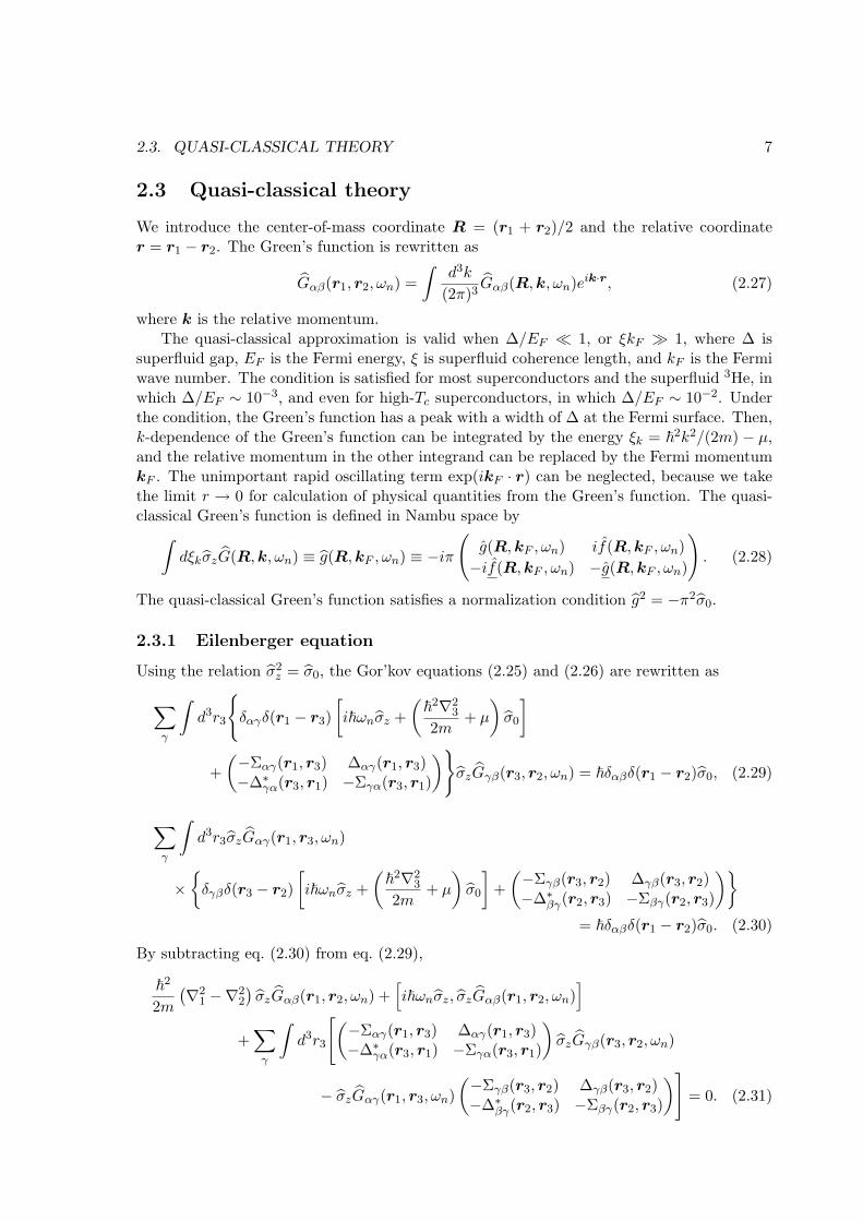
Figure 3.1: Taken from Salomaa and Volovik [35]. Phase diagram of the superfluid 3He withtemperature, pressure, and magnetic field. A region of the A-phase becomes wide and thatof the B-phase becomes narrow under a magnetic field. The A1-phase also appears under amagnetic field.
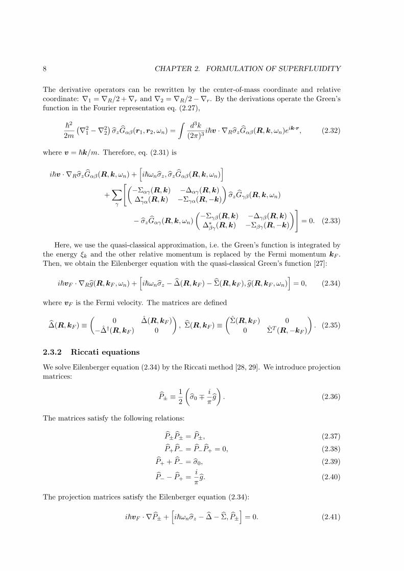
where ∆A is amplitude of the OP toward the antinode direction. m and n are orthogonal,and l-vector (l) is defined by them as
l ≡ m × n. (3.5)
l-vector signifies the direction of the orbital angular momentum, or orbital chirality, andpoints to a point node (Fig. 3.2). d-vector (d) is perpendicular to the spin S of a Cooperpair, namely, d · S = 0.
The superfluid 3He in the B-phase is in the Balian-Werthamer (BW) state [38]. The BWstate has the total angular momentum J = L+S = 0. The OP in the BW state is describedby
Aµi = ∆BRµi(n, θ), (3.6)
where Rµi(n, θ) is a rotation matrix with a rotation axis n and a rotation angle θ about n.The rotation matrix gives the relative angle between the orbital momentum and d-vector.The BW state has an isotropic full gap with amplitude ∆B.
The superfluid 3He in the A1-phase is in the spin polarized state by a magnetic field. Theorbital state is the same as that in the ABM state.
3.1. SUPERFLUID 3HE 13
point node
ΔA
l
mn
Figure 3.2: Relation between l-vector and a point node of the OP in the ABM state, where∆A is amplitude of the OP toward the antinode direction.
3.1.1 Texture
Spatial structure of the OP, namely texture, is fully characterized by l-vector and d-vectorfor the A-phase, and n-vector and θ-angle for the B-phase. The texture is constructed byvortices or boundary conditions in the restricted geometry, such as cylindrical geometry orslab (parallel plate) geometry.
For the A-phase, l-vector must be perpendicular to the boundary of the geometry to pre-vent motion of Cooper pairs toward the boundary. In other words, a point node is touchedto the boundary to minimize loss of the condensation energy at the boundary. Relation be-tween l-vector and d-vector is fixed by dipole-dipole interaction. The dipole-dipole interactionworks l-vector and d-vector into parallel, where the characteristic length of spatial variationis the dipole coherence length ξd ∼ 10 µm. Under a magnetic field, d-vector tends to be per-pendicular to the magnetic field. The interaction by a magnetic field and the dipole-dipoleinteraction are comparable under a magnetic field ∼ 2 mT.
For the B-phase, n-vector is perpendicular to the boundary of the geometry and θ-angleis fixed to Leggett angle, namely θ = θL ≡ cos−1(−1/4) ≈ 104, by dipole-dipole interactionin the absence of a magnetic field. Under a magnetic field, the OP amplitude toward themagnetic field is suppressed. In this situation, n-vector is parallel to a magnetic field andθ-angle is fixed to
θ = cos−1
(−1
4∆‖
∆⊥
), (3.7)
where ∆‖ and ∆⊥ are parallel and perpendicular components of the OP amplitude for themagnetic field, respectively. The parallel component ∆‖ is suppressed by a magnetic field. If∆‖ vanishes by a high magnetic field, the superfluid 3He is in the planar state.
3.1.2 Half-quantum vortex
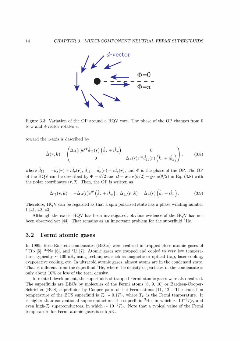
When the superfluid 3He A-phase is confined in slab geometry with a magnetic field & 2 mTperpendicular to the slab, l-vector is perpendicular to the slab and d-vector is parallel to theslab. In this situation, it is possible to form half-quantum vortices (HQVs) [39, 40]. TheHQV has a phase winding number 1/2, namely the phase of the OP changes from 0 to π,with π-rotation of d-vector around the vortex core (Fig. 3.3).
The OP for the A-phase in the slab geometry on the x-y plane with a high magnetic field
14 CHAPTER 3. MULTI-COMPONENT NEUTRAL FERMI SUPERFLUIDS
Φ=0
Φ=π
d-vector
Figure 3.3: Variation of the OP around a HQV core. The phase of the OP changes from 0to π and d-vector rotates π.
toward the z-axis is described by
∆(r,k) =
∆A(r)eiΦd↑↑(r)(kx + iky
)0
0 ∆A(r)eiΦd↓↓(r)(kx + iky
) , (3.8)
where d↑↑ = −dx(r) + idy(r), d↓↓ = dx(r) + idy(r), and Φ is the phase of the OP. The OPof the HQV can be described by Φ = θ/2 and d = x cos(θ/2) − y sin(θ/2) in Eq. (3.8) withthe polar coordinates (r, θ). Then, the OP is written as
∆↑↑(r,k) = −∆A(r)eiθ(kx + iky
), ∆↓↓(r,k) = ∆A(r)
(kx + iky
). (3.9)
Therefore, HQV can be regarded as that a spin polarized state has a phase winding number1 [41, 42, 43].
Although the exotic HQV has been investigated, obvious evidence of the HQV has notbeen observed yet [44]. That remains as an important problem for the superfluid 3He.
3.2 Fermi atomic gases
In 1995, Bose-Einstein condensates (BECs) were realized in trapped Bose atomic gases of87Rb [5], 23Na [6], and 7Li [7]. Atomic gases are trapped and cooled to very low tempera-ture, typically ∼ 100 nK, using techniques, such as magnetic or optical trap, laser cooling,evaporative cooling, etc. In ultracold atomic gases, almost atoms are in the condensed state.That is different from the superfluid 4He, where the density of particles in the condensate isonly about 10% or less of the total density.
In related development, the superfluids of trapped Fermi atomic gases were also realized.The superfluids are BECs by molecules of the Fermi atoms [8, 9, 10] or Bardeen-Cooper-Schrieffer (BCS) superfluids by Cooper pairs of the Fermi atoms [11, 12]. The transitiontemperature of the BCS superfluid is Tc ∼ 0.1TF , where TF is the Fermi temperature. Itis higher than conventional superconductors, the superfluid 3He, in which ∼ 10−3TF , andeven high-Tc superconductors, in which ∼ 10−2TF . Note that a typical value of the Fermitemperature for Fermi atomic gases is sub-µK.

3.2. FERMI ATOMIC GASES 15
Another superfluid with multi-component OP is a spinor BEC [45, 46, 47, 48] in ultracoldBose atomic gases with 23Na or 87Rb. Spinor BECs have internal degrees of freedom, namelyhyperfine spin, which appears as coupling of nuclear spin and electronic spin. Such systemcan be realized under optical traps; otherwise the hyperfine spin is polarized under magnetictraps. The OP is composed of 2F + 1-component spinor owing to the hyperfine spin F .
3.2.1 Feshbach resonance
A great advantage of the atomic gases is that interparticle interaction, or scattering length,can be tuned efficiently by Feshbach resonance. We explain the mechanism of the Feshbachresonance according to Ref. [4].
Feshbach resonance appears when total energy in an open channel matches the energy ofa bound state in a closed channel. Two particles in an initial open channel can be scatteredto an intermediate state in a closed channel, which subsequently decays to two particles inan open channel. From perturbation theory, we can expect that scattering length a has theform of a sum of terms of the type
a =∑E
C
E −Eres, (3.10)
where E is energy of the particles in the open channel, Eres is the energy of a state in theclosed channels, and C is a positive constant. Consequently, there will be large effects if theenergy E of the two particles in the entrance channel is close to the energy of a bound statein a closed channel. As we would expect from second-order perturbation theory for energyshifts, coupling between channels gives rise to a repulsive interaction if the energy of thescattering particles is greater than that of the bound state, and an attractive one if it is less.The closer the energy of the bound state is to the energy of the incoming particles in theopen channels, the larger the effect on the scattering. Then, energy summation of the righthand side of eq. (3.10) is
a = anr +C
Eth − Eres, (3.11)
where anr is a non-resonant scattering length and Eth = εα + εβ is a threshold energy ofresonant open channels with internal energy εα and εβ of atoms in the channels α and β,respectively.
Since the energies of states depend on external parameters, such as the magnetic field,these resonances make it possible to tune the effective interaction between atoms. We imaginethat the energy denominator in the second term of eq. (3.11) vanishes for a particular valueof the magnetic field, B = B0. Expanding the energy denominator about this value of themagnetic field, we find
Eth − Eres ≈ (µres − µα − µβ)(B −B0), (3.12)
where µα = −∂εα/∂B and µβ = −∂εβ/∂B are the magnetic moments of the two atoms inthe open channel, and µres = −∂Eres/∂B is the magnetic moment of the molecular boundstate. The scattering length is therefore given by
a = anr
(1 − ∆B
B −B0
), (3.13)
where ∆B is the width parameter of the resonance. A typical experimental result is shownin Fig. 3.4 [49].

16 CHAPTER 3. MULTI-COMPONENT NEUTRAL FERMI SUPERFLUIDS
Figure 3.4: Taken from Regal and Jin [49]. Scattering length versus magnetic field nearthe peak of Feshbach resonance for 40K. Amplitude of scattering length varies according to(B −B0)−1 and the sign of it changes at B0.
3.2.2 p-wave resonant Fermi atomic gases
By using magnetic Feshbach resonance, when p-wave interaction in a closed channel can beenhanced, we expect BCS superfluids by p-wave interactive Cooper pairs. In fact, thereare vigorous activities toward realizing p-wave resonant superfluids in 6Li [13, 14, 15] and40K [16, 17, 18] recently. p-wave Feshbach resonance occurs at a different magnetic field ineach hyperfine spin state of atoms, shown in Fig. 3.5 [13]. Since the spin state of superfluidityis fixed by the external magnetic field, the spin degrees of freedom are frozen, and hence onlythe orbital degrees of freedom are active. Here, the OP is characterized only by Ai, describedas
∆(r,k) =∑
i
Ai(r)ki. (3.14)
In a sense, the p-wave resonant superfluid is analogous to the “spinless” superfluid 3He A-phase.
Symmetry of the orbital state of superfluidity is broken by dipole-dipole interaction. Thedipole-dipole interaction between two alkaline atoms has the form
Hss = −α23(R · s1
)(R · s2
)− s1 · s2
R3, (3.15)
where α is the fine structure constant, si is the spin of the valence electron on an alkalineatom i, R is the interatomic separation, and R is the unit vector defining the interatomicaxis. When two dipoles are aligned head to tail they are in an attractive configuration,corresponding to R · si = 1. In contrast, when the dipoles are side by side they are in arepulsive configuration, corresponding to R · si = 0. Then, the dipole-dipole interaction actsto split the relative orbital state of two particles, depending on the projections of the orbitalangular momentum, either ml = ±1 or ml = 0, shown in Fig 3.6 [17]. This results in breakingof the degeneracy between
k± = ∓ 1√2(kx ± iky) and k0 = kz. (3.16)
3.2. FERMI ATOMIC GASES 17
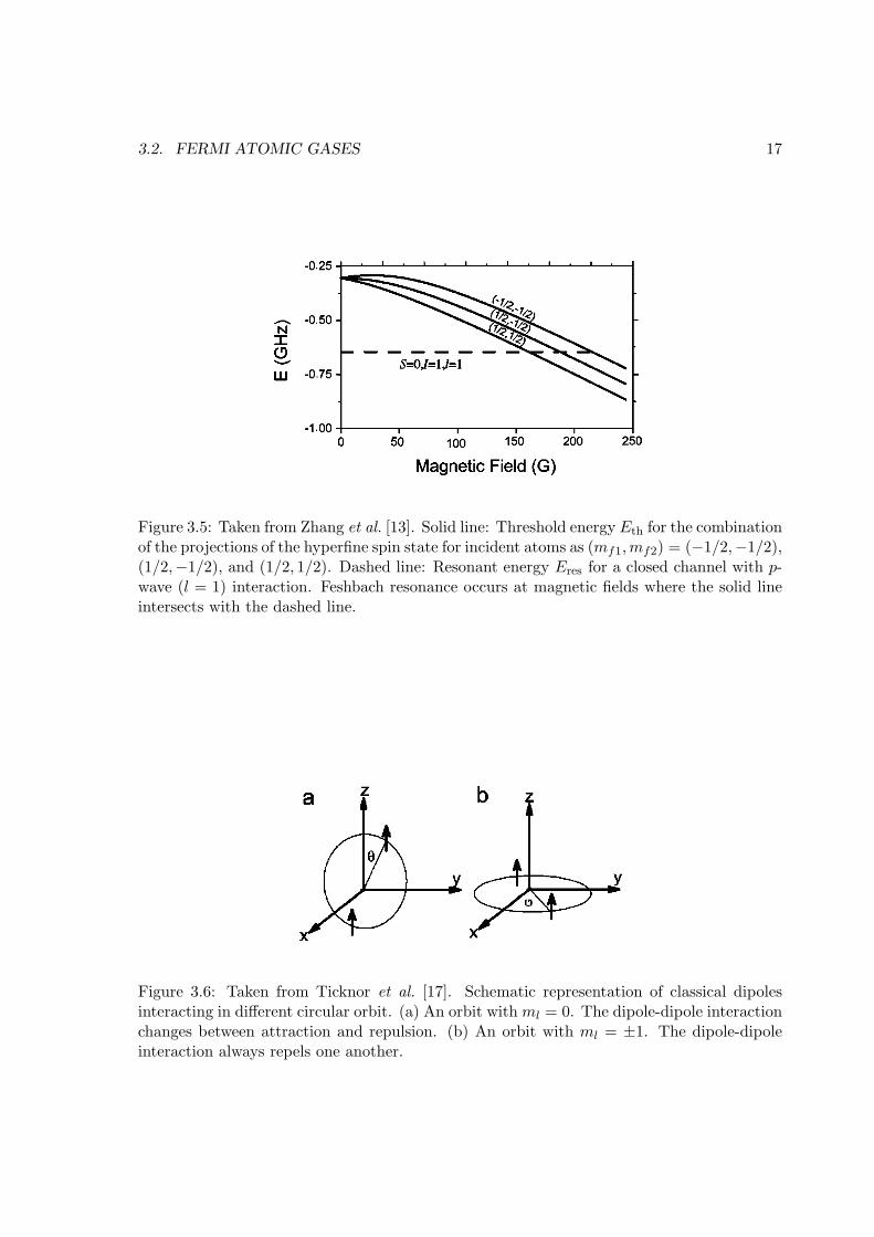
Figure 3.5: Taken from Zhang et al. [13]. Solid line: Threshold energy Eth for the combinationof the projections of the hyperfine spin state for incident atoms as (mf1,mf2) = (−1/2,−1/2),(1/2,−1/2), and (1/2, 1/2). Dashed line: Resonant energy Eres for a closed channel with p-wave (l = 1) interaction. Feshbach resonance occurs at magnetic fields where the solid lineintersects with the dashed line.
Figure 3.6: Taken from Ticknor et al. [17]. Schematic representation of classical dipolesinteracting in different circular orbit. (a) An orbit with ml = 0. The dipole-dipole interactionchanges between attraction and repulsion. (b) An orbit with ml = ±1. The dipole-dipoleinteraction always repels one another.
18 CHAPTER 3. MULTI-COMPONENT NEUTRAL FERMI SUPERFLUIDS
This split was estimated to be large for 40K by Cheng and Yip [50, 51] from the cleardifference in magnetic fields when Feshbach resonance occurs (splitting field is 0.47±0.08G [17]). For 6Li, the split may be small, because an experiment conducted in a magneticfield of H = 158.5(7) G shows no clear resonance splitting [15].
A critical difference between the superfluid 3He and the p-wave resonant superfluid ofatomic gases lies in the boundary conditions. In the superfluid 3He A-phase, l-vector is alwaysperpendicular to the boundary to minimize loss of the condensation energy at the boundary.On the other hand, since atomic gases are confined in a three-dimensional harmonic trappotential, where density of the condensation energy gradually decreases toward the outerregion, l-vector tends to align parallel to the circumference [24, 25]. This orientation isadvantageous because the condensation energy is maximally gained by allowing the pointnodes to move out from the inner region. Moreover, shapes of the trap potential is easilycontrolled, such as cigar and pancake shapes. Textures for the p-wave resonant superfluid ofatomic gases are discussed in Cap. 7.

Chapter 4
Majorana excitations
Recently, Majorana quasi-particles (QPs) and Majorana fermions have attracted much at-tention in the condensed matter physics [3] and for the application to topological quantumcomputations [52]. The Majorana QP and Majorana fermionic operator are defined by γ† = γand Ψ† = Ψ, respectively, which imply that the particle and antiparticle are identical. Ithas been proposed that the Majorana QPs bring non-Abelian statistics of vortices in chiralsuperfluids [41].
Candidate systems that exist the Majorana excitations are quite rare, e.g. spin-tripletsuperconductors or superfluids, fractional quantum Hall systems with the 5/2 filling [53, 54],interfaces between a topological insulator and an s-wave superconductor [55], and s-wavesuperfluids with particular spin-orbit interactions [56]. Majorana excitations appear at avortex or a surface, where QPs have the Andreev bound states. In this chapter, we introducethe Majorana excitations, namely γ† = γ in a vortex and Ψ† = Ψ at a surface, for spin-tripletsuperconductors of superfluids.
4.1 Majorana quasi-particle in vortex
If the self-energy in eq. (2.17) satisfies Σ†(r2, r1) = Σ(r1, r2), the following part of theBogoliubov-de Gennes (BdG) equation has the symmetry:
−σx
[K(r1, r2) + ∆(r1, r2)
]∗σx =
[K(r1, r2) + ∆(r1, r2)
]. (4.1)
By using the symmetry, the matrix uν(r) is
uν(r) =(uν(r) v∗ν(r)vν(r) u∗ν(r)
). (4.2)
Then, the BdG equation (2.17) can be reduced as∫d3r2
[K(r1, r2) + ∆(r1, r2)
](uν(r2)vν(r2)
)=(uν(r1)vν(r1)
)Eν , (4.3)
where Eν ≡ diag [Eν,↑, Eν,↓]. If we consider the energy for a spin, eq. (4.3) can be reduced as∫d3r2
[K(r1, r2) + ∆(r1, r2)
]ϕν(r2) = Eνϕν(r1), (4.4)
19

20 CHAPTER 4. MAJORANA EXCITATIONS
where ϕν ≡ [uν,1, uν,2, vν,1, vν,2]T . By using the symmetry of eq. (4.1), BdG equation is
derived another form:∫d3r2
[K(r1, r2) + ∆(r1, r2)
]σxϕ
∗ν(r2) = −Eν σxϕ
∗ν(r1). (4.5)
By comparing eqs. (4.4) and (4.5), we have one-to-one mapping between positive energystates ϕE and negative energy states ϕ−E = σxϕ
∗E . Bogoliubov QP operators are derived by
eqs. (2.12) and (2.14):
γE =∫d3rϕ†
E(r)Ψ(r)
=∫d3r
[u∗E,1(r)ψ↑(r) + u∗E,2(r)ψ↓(r) + v∗E,1(r)ψ†
↑(r) + v∗E,2(r)ψ†↓(r)
], (4.6)
γ−E =∫d3rϕ†
−E(r)Ψ(r) =∫d3r [σxϕ
∗E(r)]† Ψ(r)
=∫d3r
[vE,1(r)ψ↑(r) + vE,2(r)ψ↓(r) + uE,1(r)ψ†
↑(r) + uE,2(r)ψ†↓(r)
]. (4.7)
Therefore, we lead to the relation of the Bogoliubov QP operators γE = γ†−E . The BogoliubovQP with the zero energy is the Majorana QP, γ†0 = γ0.
Chiral p-wave superfluids have nontrivial Caroli-de Gennes-Matricon (CdGM) states [57]at a vortex. It is possible for the CdGM states to have exact zero energy states [58, 59, 60,61, 54]. We demonstrate it according to Ref. [60]. From now on, we disregard the self-energy.Then, the BdG equation (4.4) is
∫d3r2
δ(r1 − r2)[−~2∇2
2m − µ]σ0 ∆(r1, r2)
∆†(r2, r1) −δ(r1 − r2)[−~2∇2
2m − µ]σ0
ϕν(r2) = Eνϕν(r1).
(4.8)
By the Fourier transformation,[−~2∇2
2m − µ]σ0 ∆(r,k)
∆†(r,k) −[−~2∇2
2m − µ]σ0
ϕν,k(r) = Eν,kϕν,k(r). (4.9)
In weak-coupling case ∆ EF , since we can use quasi-classical approximation,(−i~vF · ∇σ0 ∆(r,k)
∆†(r,k) i~vF · ∇σ0
)ϕν,k(r) = Eν,kϕν,k(r), (4.10)
where ϕν,k(r) = ϕν,k(r)eik·r.Since many properties of the low energy excitation modes do not depend on the exact
structure of the OP and vortex core, we consider for simplicity the following paring states.For spin-singlet pairing,
∆(r,k) = iσy∆(r)(kx + iky)Nkl−Nz , (l : even), (4.11)
and for spin-triplet paring,
∆(r,k) = iσzσy∆(r)(kx + iky)Nkl−Nz , (l : odd), (4.12)
4.1. MAJORANA QUASI-PARTICLE IN VORTEX 21
vortex core x
y
φφk
φ
r
s
b
vF
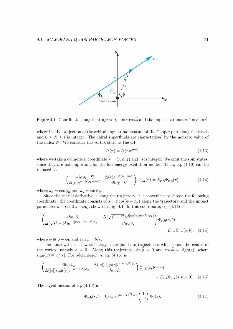
Figure 4.1: Coordinate along the trajectory s = r cos φ and the impact parameter b = r sin φ.
where l is the projection of the orbital angular momentum of the Cooper pair along the z-axisand 0 ≤ N ≤ l is integer. The chiral superfluids are characterized by the nonzero value ofthe index N . We consider the vortex state as the OP
∆(r) = ∆(r)eimφ, (4.13)
where we take a cylindrical coordinate r = (r, φ, z) and m is integer. We omit the spin states,since they are not important for the low energy excitation modes. Then, eq. (4.10) can bereduced as (
−i~vF · ∇ ∆(r)ei(Nφk+mφ)
∆(r)e−i(Nφk+mφ) i~vF · ∇
)Φν,k(r) = Eν,kΦν,k(r), (4.14)
where kx = cosφk and ky = sinφk.Since the spatial derivative is along the trajectory, it is convenient to choose the following
coordinate: the coordinate consists of s = r cos(φ− φk) along the trajectory and the impactparameter b = r sin(φ− φk), shown in Fig. 4.1. In this coordinate, eq. (4.14) is(
−i~vF∂s ∆(√s2 + b2)ei[mφ+(m+N)φk ]
∆(√s2 + b2)e−i[mφ+(m+N)φk ] i~vF∂s
)Φν,k(s, b)
= Eν,kΦν,k(s, b), (4.15)
where φ ≡ φ− φk and tan φ = b/s.The state with the lowest energy corresponds to trajectories which cross the center of
the vortex, namely b = 0. Along this trajectory, sin φ = 0 and cos φ = sign(s), wheresign(x) ≡ x/|x|. For odd integer m, eq. (4.15) is(
−i~vF∂s ∆(|s|)sign(s)ei(m+N)φk
∆(|s|)sign(s)e−i(m+N)φk i~vF∂s
)Φν,k(s, b = 0)
= Eν,kΦν,k(s, b = 0). (4.16)
The eigenfunction of eq. (4.16) is
Φν,k(s, b = 0) ∝ ei(m+N)φk2
σz
(1−i
)Φ0(s), (4.17)
22 CHAPTER 4. MAJORANA EXCITATIONS
with the zero energy, where
Φ0(s) ≡ exp[−∫ s
ds′sign(s′)∆(|s′|)
~vF
]. (4.18)
Here, exp[−(m+N)φkσy] in the Hamiltonian of eq. (4.16) gives only the boundary conditionof the eigenfunction:
Φν(φk + 2π) = (−1)m+NΦν(φk). (4.19)
When b is small, the contribution of b can be treated as perturbation. Since sin φ ≈ b/|s|,the perturbation Hamiltonian is
H′ = −bm∆(|s|)|s|
σy. (4.20)
The perturbation energy with angular momentum Lz = −kF b is
E(Lz) =
∫dsΦ†
ν,k(s, b = 0)H′Φν,k(s, b = 0)∫dsΦ†
ν,k(s, b = 0)Φν,k(s, b = 0)= −mLzω0, (4.21)
where
ω0 ≡
∫ds|Φ0(s)|2 ∆(|s|)
kF |s|∫ds|Φ0(s)|2
∼ 1~
∆2
EF. (4.22)
We should consider Lz as an operator in quantum mechanics. Then, the Hamiltoniancorresponding to energy in eq. (4.21) is
H(φk) = im~ω0∂φk. (4.23)
The Hamiltonian has the eigenfunctions
Φn,k = exp(−iEnφk
m~ω0
). (4.24)
From the boundary condition in eq. (4.19), the energy is discretized as
En = nmhω0, (N : odd), (4.25)
and
En =(n+
12
)mhω0, (N : even), (4.26)
with integer n and odd integer m. Therefore, chiral p-wave superfluids (N = 1) have theexact zero energy excitation, namely Majorana QP γ†0 = γ0, in the vortex with an oddwinding number.

4.1. MAJORANA QUASI-PARTICLE IN VORTEX 23
Figure 4.2: Taken from Ivanov [41]. Permutation of neighboring vortices. Dashed linesdenote branch cuts of the phase jumping by 2π.
4.1.1 Non-Abelian statistics
A pair of conventional fermionic creation and annihilation operators span a 2D Hilbert spacebecause their square vanishes. This is not true for the Majorana operators because γ2
i =γiγ
†i 6= 0. Thus, to avoid the problem when two Majorana QPs are present, we can construct
“conventional” complex fermionic creation and annihilation operators, ψ† = (γ1− iγ2)/2 andψ = (γ1 + iγ2)/2, respectively, where the normalization is chosen as γ2
i = 1. These operatorssatisfy ψ2 = ψ†2 = 0 and thus span a 2D subspace of degenerate ground states associatedwith these operators [52].
Since a Majorana QP exists in a vortex with an odd winding number for chiral p-wave su-perfluid, a pair of the vortices can construct the “conventional” complex fermionic operators.Then, the vortices with a Majorana QP obey the non-Abelian statistics [54, 41], because thefermionic operators are defined in a pair of isolated vortices. These nontrivial properties canbe utilized for a topological quantum computer [62]. Candidates of the non-Abelian vortexare a half-quantum vortex in the superfluid 3He A-phase and a singular vortex in a “spinless”p-wave resonant superfluid of Fermi atomic gases.
We can show the non-Abelian statistics of braiding for the vortices with a MajoranaQP according to Ref. [41]. We consider a system with 2n vortices, far from each other. Ifthe vortices move adiabatically slowly so that we can neglect transitions between subgaplevels, the only possible effect of such vortex motion is a unitary evolution in the space ofground states. We consider a permutation of vortices which returns vortices to their originalpositions. By the permutation of vortices, we disregard the multiparticle state which acquiresthe overall phase in order to note the change of the bound state in the vortex.
When we permute the neighboring vortices with a winding number m = 1, shown inFig. 4.2 [41], γi acquires a phase 2π, where a subscript of a Majorana QP operator indexesa host vortex. Since the wave function of the bound state in the vortex is proportional toei
φ2σz , the permutation of the vortices transforms γi and γj into −γj and γi, respectively.
Therefore, the action of Ti on Majorana QPs is defined as
Ti :
γi → γi+1,
γi+1 → −γi,
γj → γj ,
(4.27)
where j 6= i and j 6= i+ 1. Ti obeys the relation:
TiTj = TjTi, |i− j| > 1,TiTjTi = TjTiTj , |i− j| = 1,
(4.28)
shown in Fig. 4.3 [41]. The braiding statistics is defined by the unitary operators in the spaceof ground states representing the braid operations ofB2n. Since we disregard the multiparticle

24 CHAPTER 4. MAJORANA EXCITATIONS
Figure 4.3: Taken from Ivanov [41]. Defining relation for the braid group: TiTi+1Ti =Ti+1TiTi+1. The manner of crossings is important.
state, the permutation of the vortices with a Majorana QP is projected from the braid groupB2n. The explicit formulas for this representation may be written in terms of fermionicoperators. For the purpose, we need to construct operators τ(Ti) obeying τ(Ti)γj [τ(Ti)]
−1 =Ti(γj), where Ti(γj) is defined by (4.27). The expression for τ(Ti) is
τ(Ti) = exp(π
4γi+1γi
)=
1√2(1 + γi+1γi). (4.29)
The operators are utilized for considering operation of a topological quantum computer [52].A topological vortex qubit is defined through two pairs of vortices because the fermionicnumber is fixed to be even or odd [63].
4.2 Majorana edge fermion
In this section, we assume that the OP is uniform for simplicity. Then, eq. (4.10) is(−i~v⊥∂⊥σ0 ∆(k)
∆†(k) i~v⊥∂⊥σ0
)ϕk‖(r⊥) = Ek‖ϕk‖(r⊥), (4.30)
where subscripts ⊥ and ‖ indicate perpendicular and parallel components to a surface, re-spectively.
4.2.1 Chiral edge state
The chiral edge state is realized when the superfluid 3He A-phase is confined in a slab [64,21, 22, 23]. If there is the surface at x = 0 and l-vector and d-vector point to the z-direction,eq. (4.30) is described by
ε(k) 0 0 ∆eiφk sin θk
0 ε(k) ∆eiφk sin θk 00 ∆e−iφk sin θk −ε(k) 0
∆e−iφk sin θk 0 0 −ε(k)
ϕk‖(x) = Ek‖ϕk‖(x), (4.31)
where ∆ can be taken as real, k‖ = (ky, kz), φk and θk are the polar angle such that kx =kF cosφk sin θk, ky = kF sinφk sin θk, and kz = kF cos θk, and ε(k) = −i~vF cosφk sin θk∂x.
4.2. MAJORANA EDGE FERMION 25
By the boundary condition ϕk‖(x = 0) = 0, the wave function is
ϕk‖(r) = ϕk‖(x)eik‖·r‖ sin(kxx), (4.32)
where r‖ = (y, z). Then, eq. (4.31) can be reduced as one-dimensional Dirac equation(−i~vF cosφk sin θk∂x ∆eiφk sin θk
∆e−iφk sin θk i~vF cosφk sin θk∂x
)Φk‖(x) = Ek‖Φk‖(x). (4.33)
The eigenfunction of eq. (4.33) is
Φk‖(x) ∝ exp(− ∆x
~vF
)(1−i
), (4.34)
with energy
Ek‖ = ∆ky
kF. (4.35)
Therefore,
Φk‖(r) = ukxeik‖·r‖ sin(kxx) exp
(− ∆x
~vF
)(1−i
), (4.36)
where the normalization constant ukx satisfies
2|ukx |2∫ ∞
0dx sin2(kxx) exp
(−2∆x
~vF
)= 1. (4.37)
From eq. (2.12), field operators are expanded in terms of Bogoliubov operators γk‖,σ as(ψσ(r)ψ†
σ(r)
)=ukx sin(kxx) exp
(− ∆x
~vF
) ∑k‖,σ′
[γk‖,σ′eik‖·r‖
(1−i
)+ γ†k‖,σ′e
−ik‖·r‖
(i1
)]+ Ψbulk, (4.38)
where Ψbulk denotes the contribution from the bulk excitations. Although Ψbulk containsthe low energy states due to point nodes, their contributions are negligible if T Tc isconsidered [21]. Therefore, the chiral edge state has the Majorana fermion ψσ = iψ†
σ forT Tc.
4.2.2 Helical edge state
The helical edge state is realized for the superfluid 3He B-phase [65, 66, 67, 68]. We considerthat there is the surface at x = 0 and the rotation matrix of the OP is R(x, θL). If we rotatethe spin coordinate by the Leggett angle θL around the x-axis, the OP is described by
∆(k) =(
∆(− cos θk + i cosφk sin θk) ∆ sinφk sin θk
∆sinφk sin θk ∆(cos θk + i cosφk sin θk)
), (4.39)
where kx = kF cos θk, ky = kF cosφk sin θk, and kz = kF sinφk sin θk with −π/2 ≤ θk ≤ π/2.Then, eq. (4.30) is described by(
ε(k)σ0 ∆(k)∆†(k) −ε(k)σ0
)ϕk‖(x) = Ek‖ϕk‖(x), (4.40)
26 CHAPTER 4. MAJORANA EXCITATIONS
where ε(k) = −i~vF cos θk∂x. By the boundary condition ϕk‖(x = 0) = 0, the wave functionis
ϕk‖(r) = ϕk‖(x)eik‖·r‖ sin(kxx). (4.41)
For energy eigenvalue of the up-spin state
Ek‖,↑ = −∆sin θk, (4.42)
the eigenfunction is given by
ϕk‖,↑(x) ∝ exp(− ∆x
~vF
)sin φk+π
2
i cos φk+π2
i sin φk+π2
cos φk+π2
. (4.43)
For the energy eigenvalue of the down-spin state
Ek‖,↓ = ∆sin θk, (4.44)
the eigenfunction is given by
ϕk‖,↓(x) ∝ exp(− ∆x
~vF
)cos φk+π
2
−i sin φk+π2
i cos φk+π2
− sin φk+π2
. (4.45)
Therefore,
ϕk‖,↑(r) = ukxeik‖·r‖ sin(kxx) exp
(− ∆x
~vF
)sin φk+π
2
i cos φk+π2
i sin φk+π2
cos φk+π2
, (4.46)
and
ϕk‖,↓(r) = ukxeik‖·r‖ sin(kxx) exp
(− ∆x
~vF
)cos φk+π
2
−i sin φk+π2
i cos φk+π2
− sin φk+π2
. (4.47)

4.2. MAJORANA EDGE FERMION 27
From eq. (2.12), field operators are expanded in terms of Bogoliubov operators γk‖,σ as
ψ↑(r)ψ↓(r)ψ†↑(r)
ψ†↓(r)
= ukx sin(kxx) exp(− ∆x
~vF
)
×∑k‖
eik‖·r‖
γk‖,↑
sin φk+π
2
i cos φk+π2
i sin φk+π2
cos φk+π2
+ γk‖,↓
cos φk+π
2
−i sin φk+π2
i cos φk+π2
− sin φk+π2
+ e−ik‖·r‖
γ†k‖,↑
−i sin φk+π
2
cos φk+π2
sin φk+π2
−i cos φk+π2
+ γ†k‖,↓
−i cos φk+π
2
− sin φk+π2
cos φk+π2
i sin φk+π2
+ Ψbulk. (4.48)
We can disregard gapped modes from a bulk, where energy is greater than ∆, when T Tc.Therefore, the helical edge state has the Majorana fermion ψ↑ = −iψ†
↑ and ψ↓ = iψ†↓ for
T Tc.

Chapter 5
Superfluid 3He in a cylinder
In this chapter, we discuss the textures of the superfluid 3He A-phase confined in a narrowcylinder [19, 20]. It is known that in the absence of field, the Mermin-Ho (MH) texture [69, 70]is stable under confined geometries at rest where spontaneous mass current flows along theboundary wall. This MH texture is so generic and stable topologically, thus characteristicto multi-component order parameter (OP) superfluids. It exists even in the spinor BEC [71,72, 73, 74]. However, as the confining system becomes smaller and comparable to theircharacteristic length scale ∼ ξd (' 10 µm), the texture formation becomes difficult due tothe kinetic energy penalty, leading to destabilization of MH. Similarly MH becomes unstableunder magnetic fields whose order is Hd (' 2 mT) [75, 76]. It is not known theoreticallyand experimentally what exactly condition is needed for that and what kind of texture isstabilized in such a situation.
Here we are going to solve this problem in connection with the on-going experimentsperformed in ISSP, Univ. of Tokyo. They use two narrow cylinders with radii R=50 µmand 115 µm filled with 3He A-phase. These two kinds of cylinders are rotated up to themaximum rotation speed Ω=11.5 rad/s under a field applied along the rotation axis z andpressure P=3.2 MPa. They monitor the NMR spectrum to characterize textures created ina sample. So far the following facts are found [77, 78, 79, 80, 81]:(1) At rest an un-identified texture is seen for both samples with R=50 µm and 115 µm.The texture, which has a characteristic resonance spectrum, persists down to the lowesttemperature T/Tc=0.7, below which the B-phase starts to appear, from the onset temperatureTc=2.3 mK. Thus the ground state in those narrow cylinders is this un-identified texture.(2) Upon increasing Ω this texture is eventually changed into the MH texture which wasidentified before for R=115 µm by the same NMR experiment [79]. The critical rotationspeed Ωc ∼ 0.5 rad/s, which is identified as a sudden intensity change of the main peak inthe resonance spectrum.(3) With further increasing Ω the so-called continuous unlocked vortex (CUV) are identifiedfor R=115 µm sample. The successive transitions from the MH to one CUV, two CUVs,etc., in high rotation regions are explained basically by Takagi [82] who solves the same GLfunctional as in this chapter. However, the calculations are assumed to be the A-phase in thewhole region. Thus the following calculation is consistent with those by Takagi [82]. Thosesuccessive transitions are absent in R=50 µm sample because the estimated critical Ω forCUV exceeds the maximum rotation speed 11.5 rad/s in the rotating cryostat in ISSP.(4) The un-identified texture for R=115 µm sample stable at rest and under low rotationsexhibits a hysteretic behavior about ±Ω rotation sense [78], meaning that this texture with
29
30 CHAPTER 5. SUPERFLUID 3HE IN A CYLINDER
l-texture
d-texture
MH RD PA
ax rd hb
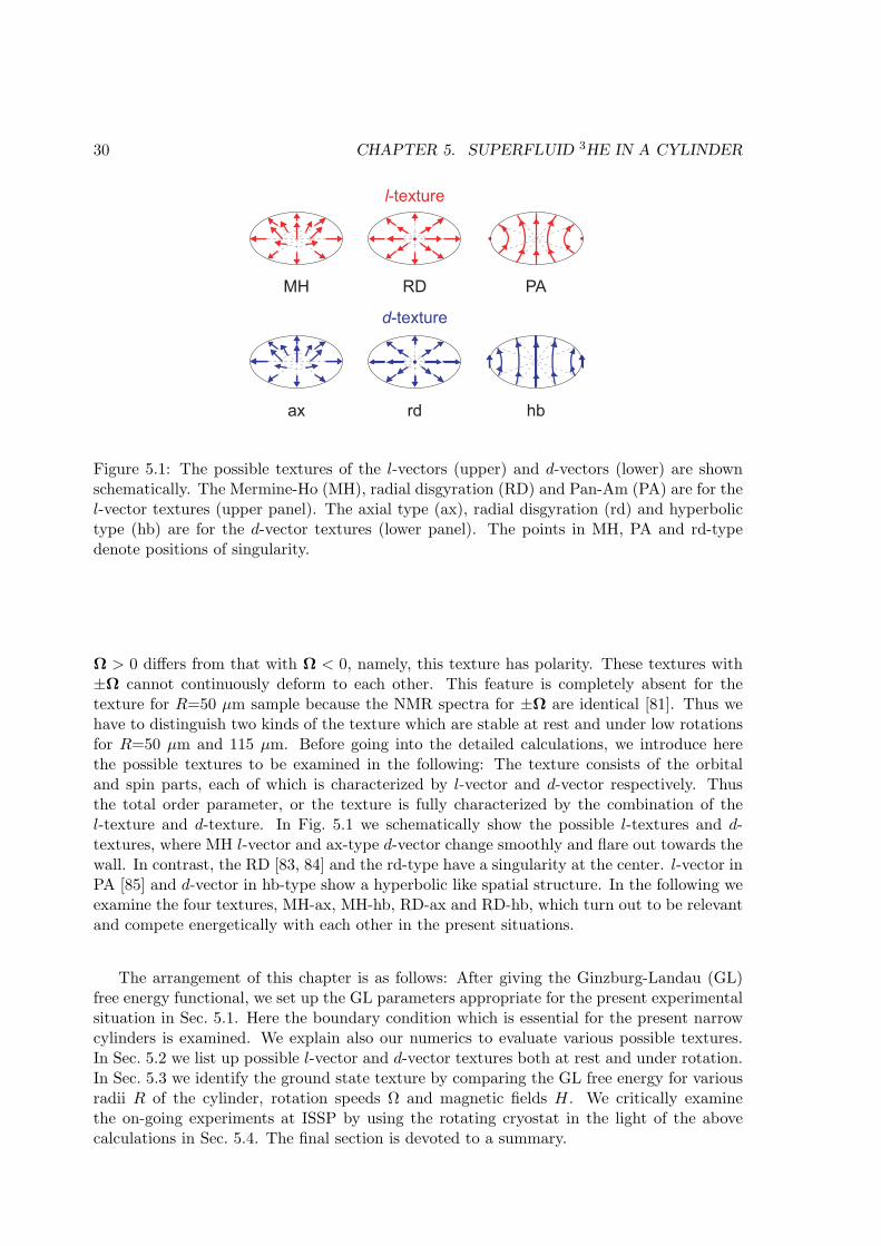
Figure 5.1: The possible textures of the l-vectors (upper) and d-vectors (lower) are shownschematically. The Mermine-Ho (MH), radial disgyration (RD) and Pan-Am (PA) are for thel-vector textures (upper panel). The axial type (ax), radial disgyration (rd) and hyperbolictype (hb) are for the d-vector textures (lower panel). The points in MH, PA and rd-typedenote positions of singularity.
Ω > 0 differs from that with Ω < 0, namely, this texture has polarity. These textures with±Ω cannot continuously deform to each other. This feature is completely absent for thetexture for R=50 µm sample because the NMR spectra for ±Ω are identical [81]. Thus wehave to distinguish two kinds of the texture which are stable at rest and under low rotationsfor R=50 µm and 115 µm. Before going into the detailed calculations, we introduce herethe possible textures to be examined in the following: The texture consists of the orbitaland spin parts, each of which is characterized by l-vector and d-vector respectively. Thusthe total order parameter, or the texture is fully characterized by the combination of thel-texture and d-texture. In Fig. 5.1 we schematically show the possible l-textures and d-textures, where MH l-vector and ax-type d-vector change smoothly and flare out towards thewall. In contrast, the RD [83, 84] and the rd-type have a singularity at the center. l-vector inPA [85] and d-vector in hb-type show a hyperbolic like spatial structure. In the following weexamine the four textures, MH-ax, MH-hb, RD-ax and RD-hb, which turn out to be relevantand compete energetically with each other in the present situations.
The arrangement of this chapter is as follows: After giving the Ginzburg-Landau (GL)free energy functional, we set up the GL parameters appropriate for the present experimentalsituation in Sec. 5.1. Here the boundary condition which is essential for the present narrowcylinders is examined. We explain also our numerics to evaluate various possible textures.In Sec. 5.2 we list up possible l-vector and d-vector textures both at rest and under rotation.In Sec. 5.3 we identify the ground state texture by comparing the GL free energy for variousradii R of the cylinder, rotation speeds Ω and magnetic fields H. We critically examinethe on-going experiments at ISSP by using the rotating cryostat in the light of the abovecalculations in Sec. 5.4. The final section is devoted to a summary.
5.1. FORMULATION 31
5.1 Formulation
5.1.1 Ginzburg-Landau functional for the superfluid 3He
The OP of the superfluid 3He is given by [2]
∆(r,k) = (iσσy) · ∆(r,k), (5.1)
with the Pauli matrix σ in spin space. The ∆ can be expanded in orbital momentumdirections,
∆µ(r,k) = Aµi(r)ki, (5.2)
where Aµi(r) is a complex 3 × 3 matrix with a spin index µ and an orbital index i. Therepeated index implies summation over x, y, and z. Thus superfluid 3He is characterizedrank-2 tensor components Aµi inherent in the p-wave pairing (L = 1) with spin S = 1, whereµ and i denote cartesian coordinates of the spin and orbital spaces, respectively.
In order to understand the stable texture at rest and lower rotations, we examine thestandard GL functional, which was written down in the 1970’s. The parameters in thefunctional are well established thanks to the intensive theoretical and experimental studiesover thirty years [86, 87, 88, 89, 90]. Namely, we start with the following GL form written interms of the tensor A forming OP of p-wave pairing. The most general GL functional densityfbulk for the bulk condensation energy up to fourth order is written as
fbulk = −αA∗µiAµi + β1A
∗µiA
∗µiAνjAνj + β2A
∗µiAµiA
∗νjAνj+β3A
∗µiA
∗νiAµjAνj
+β4A∗µiAνiA
∗νjAµj+β5A
∗µiAνiAνjA
∗µj , (5.3)
which is invariant under spin and real space rotations in addition to the gauge invarianceU(1)×SO(S)(3)×SO(L)(3). The coefficient α(T ) of the second order invariant is T -dependentas usual, and the fourth order terms have five invariants with coefficients βj in general. Thegradient energy consisting of the three independent terms is given by
fgrad = K1(∂∗i A∗µj)(∂iAµj) +K2(∂∗i A
∗µj)(∂jAµi) +K3(∂∗i A
∗µi)(∂jAµj). (5.4)
where ∂i = ∇i − i(2m3/~)(Ω × r)i with the angular velocity Ω ‖ z, which is parallel to thecylinder long axis and Ω > 0 means the counter clock-wise rotation. In addition, there arethe dipole and magnetic field energies:
fdipole = gd
(A∗
µµAνν +A∗µνAνµ − 2
3A∗
µνAµν
), (5.5)
ffield = gmHµA∗µiHνAνi. (5.6)
In the A-phase the spin and orbital parts of the OP are factorized, i.e. Aµi = dµAi, wherethe spin part is denoted by dµ and the orbital part by Ai. The d is a unit vector. We candescribe the Anderson-Brinkman-Morel (ABM) and polar state under this notation. Now,eqs. (5.3) – (5.6) are rewritten as
fbulk = −αA∗iAi + β13A
∗iA
∗iAjAj + β245A
∗iA
∗jAiAj , (5.7)
fgrad = K1(∂∗i dµA∗j )(∂idµAj) +K2(∂∗i dµA
∗j )(∂j dµAi) +K3(∂∗i dµA
∗i )(∂j dµAj), (5.8)
fdipole = gd
[dµdν
(A∗
µAν +A∗νAµ
)− 2
3A∗
νAν
], (5.9)
ffield = gmA∗iAi
(d · H
)2, (5.10)

32 CHAPTER 5. SUPERFLUID 3HE IN A CYLINDER
where β13 = β1 + β3, and β245 = β2 + β4 + β5.The coefficients α, βj , Kj , gm, and gd are determined by Thuneberg [91] and Kita [92] as
follows. The weak-coupling theory gives
α =N(0)
3
(1 − T
Tc
)≡ α0
(1 − T
Tc
), (5.11)
−2βWC1 = βWC
2 = βWC3 = βWC
4 = −βWC5 =
7ζ(3)N(0)120(πkBTc)2
, (5.12)
K1 = K2 = K3 =7ζ(3)N(0)(~vF )2
240(πkBTc)2≡ K, (5.13)
where N(0) and vF are the density of states per spin and the Fermi velocity, respectively.The coefficients α0 and K are estimated by eqs. (5.11) and (5.13) by using the values of N(0),Tc and vF which are determined experimentally by Greywall [88] within the weak-couplingtheory. It is known that strong-coupling corrections for βj are needed to stabilize A-phase,and we use the βj values estimated by Sauls and Serene [87] theoretically. The strong-coupling corrections of β13 and β245 which are coefficients in Eq. (5.7) have good agreementwith the corrections evaluated from experimental data [90]. The value of gd is [89]
gd =µ0
40
(γ~N(0) ln
1.1339 × 0.45TF
Tc
)2
, (5.14)
where µ0 and γ denote the permeability of vacuum and the gyromagnetic ratio, respectively,and TF is the Fermi temperature defined by TF ≡ 3n/4N(0)kB with the density n. Finally,gm is given within the weak-coupling expression by
gm =7ζ(3)N(0)(γ~)2
48 [(1 + F a0 )πkBTc]
2 , (5.15)
with F a0 the Landau parameter taken from Wheatley [86] but corrected for the newly deter-
mined effective mass [88].We set all the GL parameters to correspond to the above experimental pressure P=3.2
MPa, which are summarized as
α0 =N(0)
3= 3.81 × 1050J−1m−3,
β1 = −3.75 × 1099J−3m−3,
β2 = 6.65 × 1099J−3m−3,
β3 = 6.56 × 1099J−3m−3,
β4 = 5.99 × 1099J−3m−3,
β5 = −8.53 × 1099J−3m−3,
K = 4.19 × 1034J−1m−1,
gd = 5.61 × 1044J−1m−3,
gm = 1.35 × 1044J−1m−3(mT)−2,
2m3
~= 9.51 × 10⁷m−2s.

5.1. FORMULATION 33
Corresponding to these parameters, the dipole field is estimated as Hd =√gd/gm ∼ 2 mT,
which is a characteristic magnetic field where the dipole and magnetic field energies becomesame order.
The stable texture can be found by minimizing total free energy,
F =∫d3rf(r) =
∫d3r(fbulk + fgrad + fdipole + ffield). (5.16)
We have identified stationary solutions by numerically solving the variational equations:δf(r)/δdµ(r) = 0, δf(r)/δAi(r) = 0 in cylindrical systems, assuming the uniformity towardsthe z direction. The height of the cylinders used in ISSP experiments are ∼3 mm, whichallows us to adopt this assumption. Thus we obtain the stable d-textures and l-textures.Namely, we solve the coupled GL equations in two dimensions. The l-vector is defined as
li ≡ −iεijkA∗
jAk
|∆|2, (5.17)
where εijk is totally antisymmetric tensor and |∆|2 = A∗iAi is the squared amplitude of OP.
The mass current is given by
ji ≡4m3K
~Im(A∗
j∇iAj +A∗j∇jAi +A∗
i∇jAj). (5.18)
Here we expand the orbital part of the OP in the basis of spherical harmonics Ylm (l = 1,m =−1, 0, 1) for ease to express the initial configuration of the l-textures;
A(p) = A+p+ +A0p0 +A−p−, (5.19)
where p± = ∓ (px ± ipy) /√
2, p0 = pz and A± = ∓ (Ax ∓ iAy) /√
2, A0 = Az.It is noted that the characteristic length associated with the dipole energy is given by
ξd =√K/gd, which is estimated to be an order of 10 µm. In contrast, the usual coherence
length is ξ =√K/α = ξ0/
√1 − T/Tc, where the coherence length at zero temperature
ξ0 ∼ 0.01 µm. These two length scales differ by three orders of magnitude which causesgreat difficulty to handle the problem involved both scales simultaneously. This is indeedour problem. The radial disgyration (RD) has a phase singularity at the center where thel-vector vanishes around ξ-scale region while MH has no singularity and l-vector is non-vanishing everywhere whose spatial variation is characterized by ξd. In order to comparetwo energies, we need to handle two scales simultaneously. Since at the boundary l-vectoris constrained such that it is always perpendicular to the wall, thus RD and MH exhibit asimilar l-vector texture, differing only around the center of a cylinder. We evaluate possiblel-textures RD and MH in combination with d-textures; axial type (ax) and hyperbolic type(hb). The radial disgyration of d-texture (rd) is neglected since it has a singularity wheresuperfluidity is broken. Namely, we mainly examine four kinds of texture, RD-ax, RD-hb,MH-ax and MH-hb in addition to the Pan-Am (PA) only for smaller systems in this paper.Those textures, we believe, exhausts all relevant stable textures. There is no other textureknown in literature [2].
5.1.2 Numerics and boundary condition
The numerical computations have been done by using polar coordinates (r, θ). The radialdirection r is discretized into 1000 meshes for R=50 µm system and 2300 meshes for R=115

34 CHAPTER 5. SUPERFLUID 3HE IN A CYLINDER
µm while the azimuthal angle θ is discretized in 180 points. Thus the total lattice points are1000×180 and 2300×180 in (r, θ) coordinate system for R=50 µm and R=115 µm respec-tively. The average lattice spacing is an order of 5ξ0 for both cases, which is fine enough toaccurately describe a singular core in RD. Note that we are considering high temperatureregion, ξ(T = 0.95Tc) ∼ 4.5ξ0 ∼ 45 nm while our lattice spacing is 50 nm. The advantagesof using (r, θ) coordinate system over the rectangular (x, y) system are (1) we can reduce thetotal lattice points, keeping the numerical accuracy and (2) it is easy to take into account theboundary condition at the wall where the l-vector orients along the perpendicular directionto the wall, namely the radial direction r. The disadvantage is that we cannot describe thePan-Am (PA) type configuration for the l-vector.
On each lattice points the nine variational parameters are assigned, coming from thecomplex variable Ai(i = x, y, z) and the real three dimensional vector dµ(µ = x, y, z). Thesenine parameters are determined iteratively and self-consistently by solving the coupled GLequations. One solution needs ∼7 days for R=50 µm system and ∼20 days for R=115µm system by using OpenMP programming on a XEON 8 core machine. The applied fieldH=21.6 mT is taken for all calculation except for subsection 5.3.2.
In this chapter, we assume a specular boundary wall. At the wall, the components ofthe OP having momentum parallel to the wall are not affected, whereas the perpendicularcomponent to the wall is suppressed completely. Realistic walls may be diffusive boundarieswhere the parallel components may be also reduced. However, since it is difficult to accuratelyestimate the reductions of OP, we apply the specular boundary condition in this chapter.The diffusive boundary condition is favorable for the PA texture over the RD, since thecondensation energy which is cost by singularities at the wall decreases. For small radiuscases R ≤ 20 µm, we confirm that the PA texture is not stable compared to the RD (seesubsection 5.2.3 for detail). For large radius cases, we examine the PA texture by consideringthe actual experimental results, because the numerical calculation for the PA texture isdifficult.
5.2 Stable textures
In order to help identifying the possible texture realized in narrow cylinders (R=50 µm and115 µm) both at rest and under rotation, we first examine the detailed spatial structuresfor each texture, which consists of the l-vector and d-vector before discussing the relativestability among them under actual experimental setups.
5.2.1 Radial disgyration (RD)
The RD is characterized by having a singularity at the center where A±(r = 0) = 0 andA0(r = 0) 6= 0. Thus the vortex core is filled by A0 component, namely it is a polar corevortex [93]. The associated d-vector texture could be either hb-type or ax-type. The l-vectortexture can be obtained by starting with an initial configuration:
A+(r, θ) =∆A
2tanh
(r
ξ
)e−iθ,
A0(r, θ) =∆A√
2, (5.20)
A−(r, θ) =∆A
2tanh
(r
ξ
)eiθ,

5.2. STABLE TEXTURES 35
(a)
-0.0003
0
0.0003
(d)
-0.06
0
0.06
(c)
(b)
x, y [µm]
l zj θ
[1
0-1
2Jm
-3(m
/s)-
1]
-0.02
-0.04
0
0.5
1.0
0 3010 4020
-0.06
-0.5
(e)
(f)
0
50x
y
Figure 5.2: Stable textures and current for RD-hb under R=50 µm and T/Tc = 0.95. (a)l-vector textures at rest. (b) d-vector textures at rest. (c) l-vector textures at Ω=3 rad/s.(d) d-vector textures at Ω=3 rad/s. The arrows indicate the x-y component and color codesdenote its z component. (e) The z component of the l-vector and (f) the current jθ alongthe radial direction r from the center. The red lines are at rest and blue lines are Ω=3 rad/s.The solid (dashed) lines are along x- (y-)axis.
where ∆A is the amplitude of OP in the bulk region far away from the center and boundary.The combination of the winding number in RD is (w+, w0, w−) = (−1, 0, 1), where w+, w0
and w− are the winding numbers for A+, A0 and A− respectively. The A± components aresuppressed over ξ distance from the center while the A0 component is larger in the center.Since at the center only the A0 component is non-vanishing, the polar state is realized thereas mentioned before. It is seen from eq. (5.17) that in this RD form lz = 0 because of|A+| = |A−|.
In Fig. 5.2 we show the results of the stable RD-hb textures for R=50 µm, whereFigs. 5.2(a) and 5.2(b) at rest and Figs. 5.2(c) and 5.2(d) at Ω=3 rad/s. It is seen thatl-vectors flare out from the center and point perpendicular to the wall (Fig. 5.2(a)). Thed-vectors point almost to the horizontal direction (the x-axis), and curve near the wall(Fig. 5.2(b)), because the dipole interaction tends to align the d-vector parallel to the l-vector direction. We call it “hyperbolic” (hb). The l-vectors do not point completely to theradial direction, but are twisted slightly due to the dipole interaction. Since the l-vectors arestrongly constrained by the boundary condition, they should be perpendicular to the wallso as to suppress the perpendicular motion of the Cooper pair. In other words, point nodeswhich locate to the l-vector direction should direct to the wall, thus saving the condensationenergy loss. Note that there is no z-components for both l and d in RD-hb at rest. It willbe soon shown that this RD texture is most stable at rest and lower rotations in narrowcylinders.
Once the rotation is turned on, the l-vectors and d-vectors now acquire the z components.It is seen from Fig. 5.2(c) that the l-vectors tend to point the negative z direction, recognized
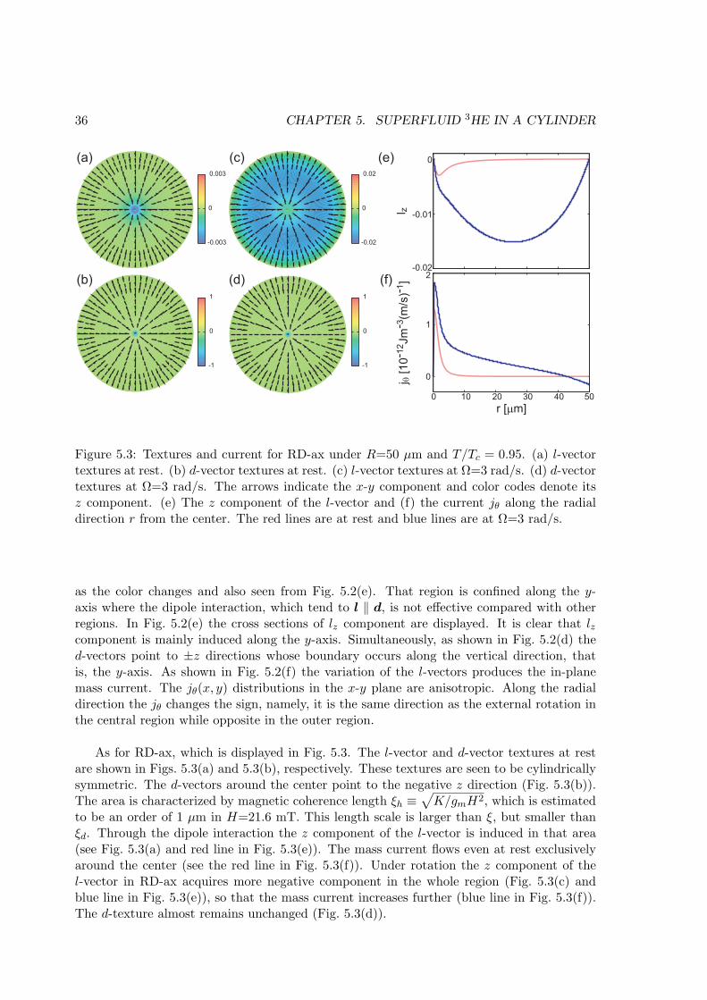
36 CHAPTER 5. SUPERFLUID 3HE IN A CYLINDER
-0.02
0
0.02
-1
0
1
(a)
(d)
(c)
(b)
r [µm]l z
j θ [
10
-12Jm
-3(m
/s)-
1]
-0.02
-0.01
0
2
1
0 3010 4020
(e)
(f)
0
-0.003
0
0.003
-1
0
1
50
Figure 5.3: Textures and current for RD-ax under R=50 µm and T/Tc = 0.95. (a) l-vectortextures at rest. (b) d-vector textures at rest. (c) l-vector textures at Ω=3 rad/s. (d) d-vectortextures at Ω=3 rad/s. The arrows indicate the x-y component and color codes denote itsz component. (e) The z component of the l-vector and (f) the current jθ along the radialdirection r from the center. The red lines are at rest and blue lines are at Ω=3 rad/s.
as the color changes and also seen from Fig. 5.2(e). That region is confined along the y-axis where the dipole interaction, which tend to l ‖ d, is not effective compared with otherregions. In Fig. 5.2(e) the cross sections of lz component are displayed. It is clear that lzcomponent is mainly induced along the y-axis. Simultaneously, as shown in Fig. 5.2(d) thed-vectors point to ±z directions whose boundary occurs along the vertical direction, thatis, the y-axis. As shown in Fig. 5.2(f) the variation of the l-vectors produces the in-planemass current. The jθ(x, y) distributions in the x-y plane are anisotropic. Along the radialdirection the jθ changes the sign, namely, it is the same direction as the external rotation inthe central region while opposite in the outer region.
As for RD-ax, which is displayed in Fig. 5.3. The l-vector and d-vector textures at restare shown in Figs. 5.3(a) and 5.3(b), respectively. These textures are seen to be cylindricallysymmetric. The d-vectors around the center point to the negative z direction (Fig. 5.3(b)).The area is characterized by magnetic coherence length ξh ≡
√K/gmH2, which is estimated
to be an order of 1 µm in H=21.6 mT. This length scale is larger than ξ, but smaller thanξd. Through the dipole interaction the z component of the l-vector is induced in that area(see Fig. 5.3(a) and red line in Fig. 5.3(e)). The mass current flows even at rest exclusivelyaround the center (see the red line in Fig. 5.3(f)). Under rotation the z component of thel-vector in RD-ax acquires more negative component in the whole region (Fig. 5.3(c) andblue line in Fig. 5.3(e)), so that the mass current increases further (blue line in Fig. 5.3(f)).The d-texture almost remains unchanged (Fig. 5.3(d)).
5.2. STABLE TEXTURES 37
5.2.2 Mermin-Ho (MH)
The MH texture does not include singularities, being the ABM state throughout the sys-tem. The l-vector is directed to the z-axis at the center, avoiding singularities. An initialconfiguration for the l-vector texture is
A+(r, θ) =∆A
2[1 + cosβ(r)],
A0(r, θ) =∆A√
2sinβ(r)eiθ, (5.21)
A−(r, θ) =∆A
2[1 − cosβ(r)]e2iθ,
where β(r) = πr/2R varies linearly from 0 at the center to π/2 at the wall. Thus the l-vectorpoints towards the z direction at the center and the radial direction at the wall. The d-vectortexture could be either hb-type or ax-type.
The MH-hb is shown in Fig. 5.4 both at rest and under rotation. At rest the z componentof the l-vectors is non-vanishing around the center in an anisotropic manner (as seen fromFig. 5.4(a)). The anisotropy of the lz component in the x-y plane is understood in terms ofthe dipole interaction, which is shown in Fig. 5.4(c). The correlation between the l-textureand d-texture produces the anisotropic arrangements in each textural configuration. Theelongated lz component along the y direction is already explained in the previous subsection.The length scales of the lz variation towards the x and y directions are characterized by ξd andR respectively. The l-vector and the associated d-vector variations along the x-axis at y = 0around the center are shown schematically in Fig. 5.5. It is seen that since the l-vectors (redarrows) flare out from the center, the z component of the d-vector (blue arrows) changes thesign at x = 0. This configuration embedded in the hyperbolic d-texture is most advantageousby increasing the parallel portion (l ‖ d) due to the dipole interaction. Since this structureis characterized by the winding number combination (w+, w0, w−) = (0, 1, 2), it yields thespontaneous mass current at rest (red lines in Fig. 5.4(d)). Thus MH has polarity whichbreaks the symmetry for ±Ω under rotation, and jθ(x, y = 0) is larger than jθ(x = 0, y)around the center, and this relation is reversed in the outer region. Under rotation theoverall configuration of the l-vector and d-vector textures are not much changed comparedwith those at rest. The small changes of the lz component and jθ are shown in Figs. 5.4(c)and 5.4(d).
As for MH-ax shown in Fig. 5.6, the overall textures for l-vector and d-vector have cylin-drical symmetry. Note that the winding number combination (0, 1, 2) is the same as before.The l-vectors and d-vectors around the center whose length scales are characterized by ξd andξh, respectively. These two length scales also appear in jθ as clearly seen from Fig. 5.6(d),where the sharp rise corresponds to ξh and the maximum position to ξd. The lz component inFig. 5.6(c) shows gradual changes characterized by ξd. The external rotation hardly changesthese features.
5.2.3 Pan-Am texture
The l-texture in Pan-Am (PA) is characterized by the two singularities at the wall as shownschematically in Fig. 5.1. In order to stabilize the PA we start with the initial configuration

38 CHAPTER 5. SUPERFLUID 3HE IN A CYLINDER
(a)
(d)
(c)
(b)l z
j θ [10-1
2Jm
-3(m
/s)-
1]
-1
0
1
-0.005
0
0.005
x, y [µm]
1
0.8
0.6
0.4
0.2
0
5
10
00 3010 4020 50
Figure 5.4: Stable textures and current for MH-hb under R=50 µm and T/Tc = 0.95. (a)l-vector and (b) d-vector textures at rest. The arrows indicate the x-y component and colorcodes denote its z component. (c) The z component of the l-vector and (d) the current jθalong the radial direction r from the center. The red lines are at rest and blue lines are Ω=3rad/s. The solid (dashed) lines are along x- (y-)axis.
0
x
Figure 5.5: Arrangements of the l-vectors (red arrows) and d-vectors (blue arrows) for theMH-hb are shown schematically. The three pairs of arrows show schematically the variationsalong the x-axis around the center. Note that the angle between the d-vectors and the x-axisis exaggerated.

5.2. STABLE TEXTURES 39
(a)
(d)
(c)
(b)
l zj θ
[10-1
2Jm
-3(m
/s)-
1]
-1
0
1
-1
0
1
r [µm]
1
0.8
0.6
0.4
0.2
020
10
00 3010 4020 50
Figure 5.6: Textures and current for MH-ax under R=50 µm and T/Tc = 0.95. (a) l-vectorand (b) d-vector textures at rest. The arrows indicate the x-y component and color codesdenote its z component. (c) The z component of the l-vector and (d) the current jθ alongthe radial direction r from the center. The red lines are at rest and blue lines are Ω=3 rad/s.
given by
A+(r, θ) = −∆A
2(sinα− i cosα),
A0(r, θ) = i∆A√
2, (5.22)
A−(r, θ) =∆A
2(sinα+ i cosα),
with
tanα(r, θ) = − r2 sin 2θR2 + r2 cos 2θ
,
where R is the radius of the system. The angle tanα diverges at (r, θ) = (R,±π/2). Atthose positions the OP amplitudes A± must be zero so that those are avoided. Around thosepoints the phase windings are (w+, w0, w−) = (−1, 0, 1). Therefore those are analogous tothe RD in the phase structure because the singularity at the center in RD is regarded to besplit into two in PA.
We show here the stabilized PA structure for small size system R=20 µm in Fig. 5.7where the l-vector and d-vector structures are displayed. From Fig. 5.7(a) the l-vectors tendto curve near the wall to satisfy the boundary condition, which causes the curving of thed-vectors shown in Fig. 5.7(b), otherwise they are straight pointing to the x direction. Wenotice that the energy of this PA is higher than the previous four kinds of the texturesmentioned above. This is also true for smaller systems with different R’s.
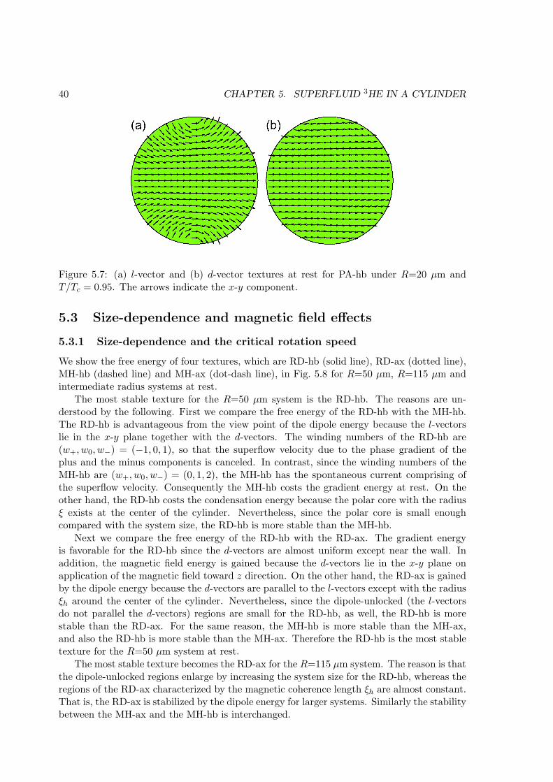
40 CHAPTER 5. SUPERFLUID 3HE IN A CYLINDER
Figure 5.7: (a) l-vector and (b) d-vector textures at rest for PA-hb under R=20 µm andT/Tc = 0.95. The arrows indicate the x-y component.
5.3 Size-dependence and magnetic field effects
5.3.1 Size-dependence and the critical rotation speed
We show the free energy of four textures, which are RD-hb (solid line), RD-ax (dotted line),MH-hb (dashed line) and MH-ax (dot-dash line), in Fig. 5.8 for R=50 µm, R=115 µm andintermediate radius systems at rest.
The most stable texture for the R=50 µm system is the RD-hb. The reasons are un-derstood by the following. First we compare the free energy of the RD-hb with the MH-hb.The RD-hb is advantageous from the view point of the dipole energy because the l-vectorslie in the x-y plane together with the d-vectors. The winding numbers of the RD-hb are(w+, w0, w−) = (−1, 0, 1), so that the superflow velocity due to the phase gradient of theplus and the minus components is canceled. In contrast, since the winding numbers of theMH-hb are (w+, w0, w−) = (0, 1, 2), the MH-hb has the spontaneous current comprising ofthe superflow velocity. Consequently the MH-hb costs the gradient energy at rest. On theother hand, the RD-hb costs the condensation energy because the polar core with the radiusξ exists at the center of the cylinder. Nevertheless, since the polar core is small enoughcompared with the system size, the RD-hb is more stable than the MH-hb.
Next we compare the free energy of the RD-hb with the RD-ax. The gradient energyis favorable for the RD-hb since the d-vectors are almost uniform except near the wall. Inaddition, the magnetic field energy is gained because the d-vectors lie in the x-y plane onapplication of the magnetic field toward z direction. On the other hand, the RD-ax is gainedby the dipole energy because the d-vectors are parallel to the l-vectors except with the radiusξh around the center of the cylinder. Nevertheless, since the dipole-unlocked (the l-vectorsdo not parallel the d-vectors) regions are small for the RD-hb, as well, the RD-hb is morestable than the RD-ax. For the same reason, the MH-hb is more stable than the MH-ax,and also the RD-hb is more stable than the MH-ax. Therefore the RD-hb is the most stabletexture for the R=50 µm system at rest.
The most stable texture becomes the RD-ax for the R=115 µm system. The reason is thatthe dipole-unlocked regions enlarge by increasing the system size for the RD-hb, whereas theregions of the RD-ax characterized by the magnetic coherence length ξh are almost constant.That is, the RD-ax is stabilized by the dipole energy for larger systems. Similarly the stabilitybetween the MH-ax and the MH-hb is interchanged.

5.3. SIZE-DEPENDENCE AND MAGNETIC FIELD EFFECTS 41
-1
-0.99999
-0.99998
-0.99997
115 80 50
R [µm]
F/|F
RD
-hb(R
)|
Figure 5.8: Size dependences of the free energies for various textures at rest. For R=50 µmRD-hb (solid line) is stable while for R=115 µm RD-ax (dotted line) becomes stable. Theother lines show MH-hb (dashed line) and MH-ax (dot-dash line).
Under rotation, the MH textures are stable because they have the spontaneous currentand they are tolerable under rotation compared with the RD textures which have very littlespontaneous current. The external rotation drives the RD-hb into the MH-hb for the R=50µm system. Similarly the most stable texture RD-ax for the R=115 µm system at restchanges into MH-hb by the rotation. Therefore l-texture and d-texture change at the criticalrotation speed.
The rotational speed changing the most stable l-texture from the RD to the MH isdefined as critical rotation speed Ωc. The Ωc obtained from the numerical calculations forthe systems with the various radii R is shown as solid circles in Fig. 5.9. The RD is themost stable l-texture from the R=5 µm to the R=115 µm systems at rest, and the MH-hbis the most stable texture under rotation. The Ωc decreases with increasing the radius ofthe systems. The numerical results of the Ωc curve upward compared with the dashed line,which is proportional to R−2.5. Therefore it is concluded that the RD is the most stabletexture up to the R→ ∞ systems at rest. Note that the results are obtained under the highmagnetic field. It has been pointed out by Buchholtz and Fetter [75, 76] that the RD is morefavorable when the radius R of the systems becomes large.
5.3.2 Magnetic field effect
So far we have fixed the magnetic field at H=21.6 mT, which is selected by experimentsat ISSP because the NMR signals are best resolved. From the theoretical point of view itis interesting to know in what weaker field MH is realized over RD. We show the resultin Fig. 5.10 where various textures are compared as a function of H for R=50 µm andT/Tc=0.95. It is found that at H=2 mT MH-ax becomes stable over RD-hb beyond whichRD-hb is always stable. Below the dipole magnetic field MH is expected to be stable overRD although it might be difficult to obtain good NMR signals in such a weak field. Thus forfeasible magnetic field region around H=21.6 mT where sensible NMR signal is detectable,RD-hb is always stable in the narrow cylinders.
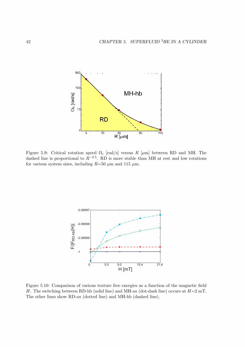
42 CHAPTER 5. SUPERFLUID 3HE IN A CYLINDER
Figure 5.9: Critical rotation speed Ωc [rad/s] versus R [µm] between RD and MH. Thedashed line is proportional to R−2.5. RD is more stable than MH at rest and low rotationsfor various system sizes, including R=50 µm and 115 µm.
-1
-0.99999
-0.99998
-0.99997
21.6 15.4 9.0 5.0 0
H [mT]
F/|F
RD
-hb(H
)|
Figure 5.10: Comparison of various texture free energies as a function of the magnetic fieldH. The switching between RD-hb (solid line) and MH-ax (dot-dash line) occurs at H=2 mT.The other lines show RD-ax (dotted line) and MH-hb (dashed line).

5.4. ANALYSIS OF EXPERIMENTS 43
Figure 5.11: Phase diagram of critical rotation speed Ωc (boundary line) and T/Tc (R=50µm). At rest RD-hb is always stable. The inset shows an example of the energy crossingbetween RD-hb (solid line) and MH-hb (dashed line) at T/Tc = 0.7, showing Ωc=1.8 rad/s.
5.4 Analysis of experiments
5.4.1 R=50 µm
In Fig. 5.11 we plot the critical rotation speed Ωc as a function of temperature T/Tc for R=50µm case. At rest RD-hb is always stable over MH-hb. Upon increasing Ω, MH-hb becomesstable at Ωc, which is an increasing function of T/Tc because the gradient energy outside thecore ∼ lnR/ξ becomes lower as approaching Tc where ξ is longer. The reason why MH-hbis advantageous over RD-hb under rotation is that MH-hb has the spontaneous current, incontrast, RD-hb has no spontaneous current. These characteristics are seen in the inset ofFig. 5.11.
NMR spectroscopy can be used to identify different topological objects of rotating su-perfluid 3He A-phase [94], namely it can be used to identify texture in a narrow cylinder.The dipole-locked (l ‖ d) and d ⊥ H regions occupying most of the condensates in thecylinder yields the main peak of NMR spectra. In the high field limit its frequency is givenby [95, 34, 2]
ω2t = ω2
L + ω2l . (5.23)
where ωL = γH is the Larmor frequency and ωl is the longitudinal resonance frequency ofthe 3He A-phase. The regions where the d-vectors are dipole-unlocked and deviate fromthe perpendicular direction to the field, generate the small satellite peaks. The resonancefrequency of a satellite is expressed in terms of a relative frequency shift R2
t , defined by theequation
ω2t = ω2
L +R2tω
2l . (5.24)
Therefore the texture in a narrow cylinder is identified by finding R2t .
In experiment of the NMR spectroscopy for various temperatures a satellite peak withR2
t ' 0.8 is observed at rest [80]. The value of R2t corresponds approximately to that by the

44 CHAPTER 5. SUPERFLUID 3HE IN A CYLINDER
-1
-0.999999
-0.999998
0 0.5 1.0 1.5 2.0
F/|F
RD
-hb(Ω
=0
)|
Ω [rad/s]Ωc
Figure 5.12: Free energy comparison of various textures for R=115 µm. RD-ax (dotted line)changes to MH-hb (dashed line) at Ωc=1.3 rad/s. The other lines show RD-hb (solid line)and MH-ax (dot-dash line).
RD-hb [96]. In the case of PA-hb, since the radius of the cylinder is much larger than thedipole coherence length, the d-vector should be parallel to the l-vector whose region occupiesthe large part of the cylinder. Therefore, PA-hb shows R2
t ' 1.0. We also notice that RD-ax gives R2
t ' 1.0 because a small area around the center of the cylinder with a radius ξhcontributes to satellite peaks. Consequently, the realized texture is definitely RD-hb, neitherPA-hb nor RD-ax. Upon increasing Ω, RD-hb changes into MH-hb. This texture has beenidentified previously by Takagi [82] who has calculated R2
t ' 0.3 for MH-hb.The precise determination of the temperature dependence of Ωc(T ) is under way exper-
imentally. Thus it is unable to check our prediction shown in Fig. 5.11 at this time. Weemphasize here, however, that the NMR spectra at low Ω and high Ω are distinctively differ-ent, therefore it is clear that the phase transition between two textures RD-hb and MH-hboccurs.
Experimentally [81] there is no hysteresis for ±Ω, indicating that the texture at rest hasno polarity to the direction of rotation. This is in agreement with our identification of RD-hbfor R=50 µm, which has no polarity.
5.4.2 R=115 µm
As shown in previous section, for the system size R=115 µm the ground state texture atrest is RD-ax which is stabler than MH-hb. The critical rotation speed Ωc=1.3 rad/s atT/Tc=0.95 is calculated as shown in Fig. 5.12. The value of Ωc roughly coincides with theISSP experiment [79].
Experimentally there is a large hysteresis behavior about ±Ω centered at Ω=0 [78], whichis contrasted with R=50 µm case mentioned above. This is understood because RD-ax haspolarity where l-vectors and d-vectors point to one of the directions ±z-axis around the centerwhich breaks ±Ω symmetry. We notice that PA-hb has no polarity.
As for the NMR spectrum at rest, they observe no distinctive satellite feature for R=115µm [80]. These facts do not contradict our identification of RD-ax, which is R2
t ∼ 1.0. Thuswe expect no satellite feature for RD-ax.

5.5. SUMMARY 45
5.5 Summary
Let us discuss the experimental facts (1)-(4) introduced in the first of this chapter.(1) We have identified the unknown texture as RD-hb for 50 µm sample and RD-ax for 115µm sample at rest and lower rotations by finding the most stable texture in those conditions.(2) Upon increasing the rotation, we found that RD changes into MH where MH was identifiedbefore by NMR resonance shape unambiguously [78] for 115 µm sample under rotations. Thisis confirmed by the present calculation. Namely, we precisely determined the critical rotationspeed Ωc from RD to MH for two samples.(3) Under further higher rotation speeds multiple MH texture is expected to appear, that is,CUV. The estimated Ω ∼ 16 rad/sec for R=50 µm [77] is too high to attain in the presentrotation cryostat in ISSP, whose maximum speed is 11.5 rad/s.(4) Our identifications of RD-hb for R=50 µm and RD-ax for R=115 µm are perfectlymatched with the experimental facts that in the former (latter) there does not exist (doexist) the hysteresis under the ±Ω rotations, namely, the former texture RD-hb has nopolarity and can change continuously under the reversal of the rotation sense. In contrast,RD-ax has a definite polarity because the d-vectors point to the negative z direction for thecounter clock-wise rotation, which never continuously change into the positive z directionwhen the rotation sense is reversed, leading to a hysteresis phenomenon.
As for the possibility of the PA texture which has not been calculated for the same sizeswith the experimental systems, the PA texture is not realized by the following reasons: (a)For the R=50 µm system the satellite position R2
t ' 1.0 for the PA texture differs from theobserved one R2
t ' 0.8 [80]. (b) For the R=115 µm system the polarity is observed [78] whilethe PA texture has no polarity.
Here we have adopted the specular boundary condition, assuming that the parallel com-ponents of the quasi-particle momentum to the wall are not affected at the wall. This may notbe the realistic experimental situation. However, we should point out that, experimentally,the coating the wall with 4He atoms does not change the experimental results mentionedabove [80]. Theoretically, the competition between RD and MH textures does not dependon the choice of the boundary conditions, either specular or diffusive, because near the walltwo textures have the same OP structures.
Because of these facts, we conclude that the un-identified texture at rest and lower rota-tions confined in narrow cylinders is RD texture. Physically RD texture with the polar coreat the center confined in a narrow cylinder under fields becomes energetically advantageousover MH, which is characterized by having the A-phase everywhere. In order to confirm ouridentification, we point out several experiments:(A) The most important prediction is the critical rotation Ωc(T ) shown in Fig. 5.11 for R=50µm. As for R=115 µm, Ωc=1.3 rad/s at T/Tc = 0.95 shown in Fig. 5.12. This can be detectedby the change of NMR spectrum because RD and MH exhibit different spectral features [94].(B) It might be quite interesting to control the texture by tuning the magnetic field H asshown in Fig. 5.10. By lowering H, MH becomes stable at rest. This controllability by Hshould be utilized to identify textures, and furthermore be used for realization of exotic andunexplored physics associated with multi-component superfluidity, such as Majorana particlein parallel plates [97, 42].(C) l-vectors in RD-hb and MH-hb, which do not point perfectly to the radial direction,exhibit a distortion or in-plane twisting as seen from Figs. 5.2(a) and 5.4(a). This ultimatelyleads to the mass current along the rotation axis; the z-direction. This non-trivial bendingcurrent (∝ ∇ × l) should be tested in a future experiment.

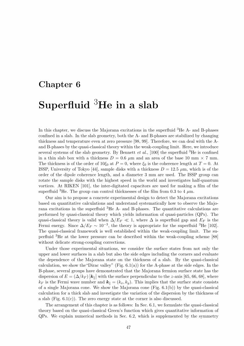
Chapter 6
Superfluid 3He in a slab
In this chapter, we discuss the Majorana excitations in the superfluid 3He A- and B-phasesconfined in a slab. In the slab geometry, both the A- and B-phases are stabilized by changingthickness and temperature even at zero pressure [98, 99]. Therefore, we can deal with the A-and B-phases by the quasi-classical theory within the weak-coupling limit. Here, we introduceseveral systems of the slab geometry. By Bennett et al., [100] the superfluid 3He is confinedin a thin slab box with a thickness D = 0.6 µm and an area of the base 10 mm × 7 mm.The thickness is of the order of 10ξ0 at P = 0, where ξ0 is the coherence length at T = 0. AtISSP, University of Tokyo [44], sample disks with a thickness D = 12.5 µm, which is of theorder of the dipole coherence length, and a diameter 3 mm are used. The ISSP group canrotate the sample disks with the highest speed in the world and investigates half-quantumvortices. At RIKEN [101], the inter-digitated capacitors are used for making a film of thesuperfluid 3He. The group can control thicknesses of the film from 0.3 to 4 µm.
Our aim is to propose a concrete experimental design to detect the Majorana excitationsbased on quantitative calculations and understand systematically how to observe the Majo-rana excitations in the superfluid 3He A- and B-phases. The quantitative calculations areperformed by quasi-classical theory which yields information of quasi-particles (QPs). Thequasi-classical theory is valid when ∆/EF 1, where ∆ is superfluid gap and EF is theFermi energy. Since ∆/EF ∼ 10−3, the theory is appropriate for the superfluid 3He [102].The quasi-classical framework is well established within the weak-coupling limit. The su-perfluid 3He at the lower pressure can be described within the weak-coupling scheme [88]without delicate strong-coupling corrections.
Under those experimental situations, we consider the surface states from not only theupper and lower surfaces in a slab but also the side edges including the corners and evaluatethe dependence of the Majorana state on the thickness of a slab. By the quasi-classicalcalculation, we show the“Dirac valley” (Fig. 6.1(a)) for the A-phase at the side edges. In theB-phase, several groups have demonstrated that the Majorana fermion surface state has thedispersion of E = (∆/kF )
∣∣k‖∣∣ with the surface perpendicular to the z-axis [65, 66, 68], where
kF is the Fermi wave number and k‖ = (kx, ky). This implies that the surface state consistsof a single Majorana cone. We show the Majorana cone (Fig. 6.1(b)) by the quasi-classicalcalculation for a thick slab and investigate the variation of the dispersion by the thickness ofa slab (Fig. 6.1(c)). The zero energy state at the corner is also discussed.
The arrangement of this chapter is as follows: In Sec. 6.1, we formulate the quasi-classicaltheory based on the quasi-classical Green’s function which gives quantitative information ofQPs. We explain numerical methods in Sec. 6.2, which is supplemented by the symmetry
47

48 CHAPTER 6. SUPERFLUID 3HE IN A SLAB
-1 0 1-1 0
1-0.6-0.4-0.2 0 0.2 0.4 0.6
kx
ky
E
-1 0 1-1 0
1-0.6-0.4-0.2 0 0.2 0.4 0.6
kx
ky
E
(a) (c)(b)
-1 0 1-1
0
1
-0.8
-0.4
0
0.4
0.8
ky
kz
ELR
Figure 6.1: Stereographic views of typical dispersion relation. (a) Dirac valley for the A-phase in a thin slab D = 8ξ0 at the left side edge “L” and the right side edge “R”. (b)Majorana cone for the B-phase in a thick slab D = 30ξ0 at the upper or lower surface. (c)Split Majorana cone for the B-phase in a thin slab D = 14ξ0 at the upper or lower surface.The units of energy and wave length are πkBTc and kF , respectively.
considerations of the quasi-classical Green’s function given in Appendix A. In Secs. 6.3 and6.4 for the A- and B-phases, we show results of the spatial structures of the order parameter(OP), the current distribution, and the local density of states (LDOS) for QPs which relatesto the Majorana modes. In Sec. 6.5, we discuss difference of the Majorana zero modes in theA- and B-phase and propose several experimental designs to observe the Majorana nature.In addition, we discuss the Majorana zero mode in the stripe phase. The final section isdevoted to a summary.
6.1 Quasi-classical theory and order parameter
We start with the quasi-classical spinful Eilenberger equation [27], which has been used forstudies of the superfluid 3He [103, 104, 99]. The low energy excitation modes at the surfaceare discretized in the order of ∆/(kFL) [64], where L is a length of the system. If L isa macroscopic length, which is much larger than k−1
F , the low energy excitation modes atthe surface can be regarded as continuous spectra. Because there is the exact zero energyexcitation at the surface of the superfluid 3He A-phase [64, 21] and B-phase [65, 66, 68], thequasi-classical theory can be used to discuss the Majorana QP.
The quasi-classical Green’s function g(r,k, ωn) is calculated using the Eilenberger equa-tion
−i~v(k) · ∇g(r,k, ωn) =[(
iωn1 −∆(r,k)∆(r,k)† −iωn1
), g(r,k, ωn)
], (6.1)
where the “ordinary hat” indicates the 2 × 2 matrix in spin space and the “wide hat”indicates the 4 × 4 matrix in Nambu and spin spaces. The quasi-classical Green’s functionis described in Nambu space by
g(r,k, ωn) = −iπ
(g(r,k, ωn) if(r,k, ωn)
−if(r,k, ωn) −g(r,k, ωn)
), (6.2)
with the direction of the relative momentum of a Cooper pair k, the center-of-mass coordinateof a Cooper pair r, and the Matsubara frequency ωn = (2n + 1)πkBT . The quasi-classical
6.1. QUASI-CLASSICAL THEORY AND ORDER PARAMETER 49
Green’s function satisfies a normalization condition g2 = −π21. The Fermi velocity is givenas v(k) = vF k on the three dimensional Fermi sphere.
We solve Eq. (6.1) by the Riccati method [29, 28, 99]. We introduce Riccati amplitudea = (1 + g)−1f and b = (1 + g)−1f related to particle- and hole-like projections of theoff-diagonal propagators, respectively. Equation (6.1) can be rewritten as Riccati equations
~v(k) · ∇a(r,k, ωn) = ∆(r,k) − a(r,k, ωn)∆(r,k)†a(r,k, ωn) − 2ωna(r,k, ωn),
−~v(k) · ∇b(r,k, ωn) = ∆(r,k)† − b(r,k, ωn)∆(r,k)b(r,k, ωn) − 2ωnb(r,k, ωn). (6.3)
The equations are solved by integration toward k for a(r,k, ωn) and toward −k for b(r,k, ωn).From the Riccati amplitude, the quasi-classical Green’s function is given as
g = −iπ(
(1 + ab)−1 00 (1 + ba)−1
)(1 − ab 2ia−2ib −(1 − ba)
). (6.4)
The self-consistent condition for the pair potential ∆(r,k) is given as
∆(r,k) = N0πkBT∑
−ωc≤ωn≤ωc
⟨V (k,k′)f(r,k′, ωn)
⟩k′, (6.5)
where N0 is the density of states in the normal state, ωc is a cutoff energy setting ωc =40πkBTc with the transition temperature Tc in a bulk, and 〈· · · 〉k indicates the Fermi surfaceaverage. The pairing interaction V (k,k′) = 3g1k ·k′ for Cooper pairs with an orbital angularmomentum L = 1, where g1 is a coupling constant. In our calculation, we use a relation
1g1N0
= lnT
Tc+ 2πkBT
∑0≤ωn≤ωc
1ωn. (6.6)
Spin-triplet OP is defined by a vectorial notation
∆(r,k) = (iσσy) · ∆(r,k), (6.7)
with the Pauli matrix σ in spin space. The complex vector ∆ is perpendicular to the spinS of a Cooper pair, namely, ∆ · S = 0. The ∆ can be expanded in orbital momentumdirections,
∆µ(r,k) = Aµi(r)ki, (6.8)
where Aµi(r) is a complex 3 × 3 matrix with a spin index µ and an orbital index i. Therepeated index implies summation over x, y, and z.
In this chapter, we discuss the chiral state in the A-phase, polar state, B-phase, andplanar state. Symbolic descriptions of the OP in their state are the following: For the chiralstate,
∆ = dz(kx + iky), (6.9)
for the polar state,
∆ = dzkx, (6.10)
50 CHAPTER 6. SUPERFLUID 3HE IN A SLAB
for the B-phase,
∆ = dxkx + dyky + dzkz, (6.11)
and for the planar state,
∆ = dxkx + dyky, (6.12)
where d-vector is perpendicular to the spin of a Cooper pair. d-vector and the momentumdirection are permitted to rotate spherically in the spin and momentum space, respectively.
By using the self-consistent quasi-classical Green’s function, the mass and spin currentsare calculated by
j(r) = mN0πkBT∑
−ωc≤ωn≤ωc
〈v(k) Im [g0(r,k, ωn)]〉k, (6.13)
jµs (r) =
~2N0πkBT
∑−ωc≤ωn≤ωc
〈v(k) Im [gµ(r,k, ωn)]〉k, (6.14)
respectively, where m is the mass of the 3He atom and gµ is a component of the quasi-classicalGreen’s function g in spin space, namely,
g =(g0 + gz gx − igy
gx + igy g0 − gz
). (6.15)
LDOS for energy E is given by
N(E, r) = 〈N(E, r,k)〉k= N0 〈Re [g0(r,k, ωn)|iωn→E+iη]〉k , (6.16)
where η is a positive infinitesimal constant and N(E, r,k) is angle-resolved LDOS. Typically,we choose η = 0.003πkBTc. For obtaining g0(r,k, ωn)|iωn→E+iη, we solve Eqs. (6.3) withη − iE instead of ωn under the pair potential obtained self-consistently.
6.2 System geometry and numerical methods
We consider a cross-section A of a slab with a thickness of D along the z-direction and amacroscopic length of L along the x-direction, shown in Fig. 6.2(a). It is assumed that thequasi-classical Green’s function and OP are homogeneous along the y-direction. We alsoassume that the surfaces of the slab are specular, where specularity is controlled by coat-ing the surface with 4He atoms [105]. Under the boundary condition, the quasi-classicalGreen’s function or the Riccati amplitude changes only the direction of the relative mo-mentum by mirror reflection at a surface Rsurf , namely, g(Rsurf ,k, ωn) = g(Rsurf ,k, ωn) ora(Rsurf ,k, ωn) = a(Rsurf ,k, ωn) and b(Rsurf ,k, ωn) = b(Rsurf ,k, ωn), where k = k−2n(n ·k)with a unit vector n which is perpendicular to the surface.
We solve Eqs. (6.3) by the numerical integration toward the k-direction for a and to-ward the −k-direction for b from the surface to the position r. Since a(Rsurf ,k, ωn) =a(Rsurf ,k, ωn), the initial value of a at a surface Rsurf is determined by the numerical inte-gration toward the k-direction from the other surface to Rsurf . Eventually, we have to solvethe numerical integration along the sufficiently long path by changing the direction from k
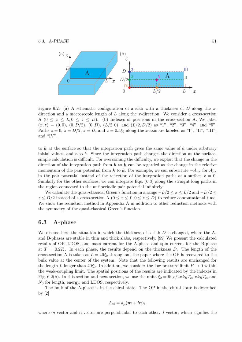
6.3. A-PHASE 51
(b)
x
z
0 L
D
A
L/2
D/22 5
I
III
II
IV 1 4
3
x
z
0 L
D
A
(a)
Figure 6.2: (a) A schematic configuration of a slab with a thickness of D along the z-direction and a macroscopic length of L along the x-direction. We consider a cross-sectionA (0 ≤ x ≤ L, 0 ≤ z ≤ D). (b) Indexes of positions in the cross-section A. We label(x, z) = (0, 0), (0, D/2), (0, D), (L/2, 0), and (L/2, D/2) as “1”, “2”, “3”, “4”, and “5”.Paths z = 0, z = D/2, z = D, and z = 0.5ξ0 along the x-axis are labeled as “I”, “II”, “III”,and “IV”.
to k at the surface so that the integration path gives the same value of a under arbitraryinitial values, and also b. Since the integration path changes the direction at the surface,simple calculation is difficult. For overcoming the difficulty, we exploit that the change in thedirection of the integration path from k to k can be regarded as the change in the relativemomentum of the pair potential from k to k. For example, we can substitute −Aµx for Aµx
in the pair potential instead of the reflection of the integration paths at a surface x = 0.Similarly for the other surfaces, we can integrate Eqs. (6.3) along the straight long paths inthe region connected to the antiperiodic pair potential infinitely.
We calculate the quasi-classical Green’s function in a range −L/2 ≤ x ≤ L/2 and −D/2 ≤z ≤ D/2 instead of a cross-section A (0 ≤ x ≤ L, 0 ≤ z ≤ D) to reduce computational time.We show the reduction method in Appendix A in addition to other reduction methods withthe symmetry of the quasi-classical Green’s function.
6.3 A-phase
We discuss here the situation in which the thickness of a slab D is changed, where the A-and B-phases are stable in thin and thick slabs, respectively. [99] We present the calculatedresults of OP, LDOS, and mass current for the A-phase and spin current for the B-phaseat T = 0.2Tc. In each phase, the results depend on the thickness D. The length of thecross-section A is taken as L = 40ξ0 throughout the paper where the OP is recovered to thebulk value at the center of the system. Note that the following results are unchanged forthe length L longer than 40ξ0. In addition, we consider the low pressure limit P → 0 withinthe weak-coupling limit. The spatial positions of the results are indicated by the indexes inFig. 6.2(b). In this section and next section, we use the units ξ0 = ~vF /2πkBTc, πkBTc, andN0 for length, energy, and LDOS, respectively.
The bulk of the A-phase is in the chiral state. The OP in the chiral state is describedby [2]
Aµi = dµ(m + in)i,
where m-vector and n-vector are perpendicular to each other. l-vector, which signifies the

52 CHAPTER 6. SUPERFLUID 3HE IN A SLAB
orbital chirality, is defined as l ≡ m × n. At the edge of a slab, since the normal orbitalcomponent to the edge vanishes, the polar state will be realized. The OP in the polar stateis described by [2]
Aµi = dµmi,
where we regard n-vector as perpendicular to the edge.In a slab cell used by Bennett et al. [100] where the thickness is 0.6 µm ≈ 8ξ0, it is
expected that the A-phase is stable at T = 0.2Tc [106]. Since the thickness D is muchshorter than the dipole coherence length ∼ 1000ξ0, d-vector, which characterizes the spinstate of the OP in the A-phase, points to the z-direction in the absence of a magnetic field aslong as l-vector is parallel to the z-axis. l-vector is parallel to the z-axis everywhere exceptnear the side edges at x = 0 and x = L in the slab shown in Fig. 6.2. The length scale of thespatial variation of l-vector is short, whose order is the coherence length. On the other hand,d-vector can not vary spatially since the order of the length scale is the dipole coherencelength. d-vector is spatially uniform even under a magnetic field [107]. In this chapter, wefix the direction of d-vector to the z-axis.
6.3.1 D = 8ξ0: Thin slab for A-phase
For D = 8, the OP is described by ∆z(x,k) = Azx(x)kx + Azy(x)ky, where the relativephase between Azx and Azy is π/2. The OP is uniform along the z-direction and variesalong only the x-direction. Since the slab is thin, the kz-component of the OP is suppressed.Note that the uniformness along the z-direction and the suppression of the kz-componentare not suppositions, but results by the self-consistent calculation. The profile of the OPalong the x-axis is shown in Fig. 6.3(a). Because of the specular boundary condition, thekx-component perpendicular to the edge becomes zero at x = 0 and x = L. In contrast, theparallel ky-component is enhanced by compensating for the loss of the kx-component at theedge, where the polar state is realized. The kx-component increases and the ky-componentdecreases toward the bulk region around x = L/2; thus, the chiral state with kx + iky isattained. We can construct l-vector as li ≡ −iεijkA∗
zjAzk/|∆|2, where εijk is the totallyantisymmetric tensor and |∆|2 = A∗
ziAzi is the squared amplitude of the OP. l-vector pointsto the z-direction in the bulk region and vanishes at the edge. Since the chiral state is realizedexcept at the edge, the Majorana fermion edge state Ψ† = Ψ exists at side edges [54, 64].
The mass current jy(x) is shown in Fig. 6.3(b). The mass current flows circularly alongthe side edge of the slab. Experimental values [88] are used as coefficients of Eq. (6.13)so that a quantitative value of the mass current is obtained. By applying a magnetic fieldperpendicular to a slab, we can produce a spin imbalance due to the Zeeman shift betweenthe up-up spin pairs and the down-down spin pairs. This results in a net spin current inaddition to the mass current.
Figure 6.3(c) shows LDOS at the edge x = 0 (the position “2” in Fig. 6.2) and thebulk x = L/2 (“5”). It is clearly seen from the line “2” for x = 0 that the LDOS witha substantial weight appears at a zero energy, corresponding to the Majorana edge mode,because the distance L between the edges is macroscopic [54, 64]. This implies that theLDOS is expressed as N(E, x = 0) = N(E = 0, x = 0) + αE2 in the vicinity of E = 0. Thefirst term comes from the Majorana edge mode, and the second term comes from the pointnode of the chiral state in the bulk A-phase. The peak at E ≈ 0.65 comes from the gap ofthe chiral state in the bulk and the peak at E ≈ 0.8 comes from the gap of the polar state atthe edge. The LDOS at x = L/2 (the line “5”) shows a typical behavior of the point node

6.3. A-PHASE 53
0
0.5
1
1.5
2
2.5
3
0 0.2 0.4 0.6 0.8 1
2
5
N(E
,x)
E
(c)
-1
-0.5
0
0.5
1
-1 -0.5 0 0.5 1
LR
E
ky
(h)
0
0.1
0.2
0.3
0.4
0.5
0 5 10 15 20
N(E
=0,x
)
x
(d)
N(E
,x=
0, θ
)
E
(e)
0
2
4
6
8
10
-1 -0.5 0 0.5 1
0
0.1
0.2
0.3
0.4
0.5
0.6
0.7
0.8
0 10 20 30 40
|Azx|
|Azy|
x
-0.3
-0.2
-0.1
0
0.1
0.2
0.3
0 10 20 30 40x
j y [kg m
-2 s
-1]
(a) (b)
N(E
,x=
0, φ
)
E
(f)
0
2
4
6
8
10
-1 -0.5 0 0.5 1-1
-0.5
0
0.5
1
-1 -0.5 0 0.5 1
E
kz
(g)-60° -30° 0° 60°30°
90°
0°
30°60°
90°
Figure 6.3: Calculated results for the A-phase with D = 8. Profiles of OP (a), and masscurrent jy (b) along the x-axis. (c) LDOS N(E, x) at “2”, and “5” defined in Fig. 6.2(b).(d) Zero energy LDOS N(E = 0, x) from the edge at x = 0 to the bulk at x = L/2. Angle-resolved LDOS N(E, x = 0, θ) with φ = 0 (e), and N(E, x = 0, φ) with θ = 90 (f). Thepeak energy of angle-resolved LDOS at the side edges as a function of kz for ky = 0 (g), andas a function of ky for kz = 0 (h), where “L” (“R”) is for the left (right) edge. In this and thefollowing figures, the units of length, energy and Aµi, LDOS, and wave length are ξ0, πkBTc,N0, and kF , respectively.
spectrum, namely, N(E, x = L/2) ∝ E2. In Fig. 6.3(d) we show the extent of the Majoranaedge mode at E = 0 toward the bulk from the edge at x = 0, which spreads over the orderof 5ξ0. The spectrum of the edge gradually changes into the bulk spectrum.
The LDOS N(E, r) is obtained by averaging the angle-resolved LDOS N(E, r,k) on theFermi surface, which has the peak at the energy of the surface Andreev bound state. Thedispersion relation of the surface Andreev bound state can be evaluated by following thepeak in each momentum direction. The angle-resolved LDOS N(E, x = 0, θ) with φ = 0
and N(E, x = 0, φ) with θ = 90 are shown in Figs. 6.3(e) and 6.3(f), respectively, whereθ is the polar angle from the kz-axis and φ is the azimuthal angle from the kx-axis on thethree-dimensional Fermi sphere. The angles and momentum directions have the relations:tan θ =
√k2
x + k2y/kz and tanφ = ky/kx. The angle-resolved LDOS is symmetric between
0 ≤ θ ≤ 90 and 180 ≥ θ ≥ 90, and between −90 ≤ φ ≤ 90 and 270 ≥ φ ≥ 90.The zero energy peaks of the angle-resolved LDOS appear if φ = 0 except for θ = 0. Thezero energy peaks come from the zero energy Andreev bound state of QPs at the edge. TheQPs without the ky-component have the zero energy Andreev bound state because they feelthe π-phase shift of the pair potential for the relative momentum from (kx, ky = 0, kz) to(−kx, ky = 0, kz). This is clear from the Eilenberger equation (6.1) since the quasi-classicalGreen’s function g(k) depends on only the k-component of the pair potential kx + iky. Theangle-resolved LDOS is asymmetric with respect to E = 0 (Fig. 6.3(f)) because the superfluidstate in the A-phase has the chirality [61]. The asymmetric angle-resolved LDOS is relatedto the mass current.
The peak energy of angle-resolved LDOS at the side edges as a function of kz for ky = 0and as a function of ky for kz = 0 is shown in Figs. 6.3(g) and 6.3(h), respectively. It is foundthat the energy is dispersionless along the kz-axis and two linear dispersions appear nearE = 0 along the ky-axis, where each dispersion comes from the left (x = 0) and right (x = L)
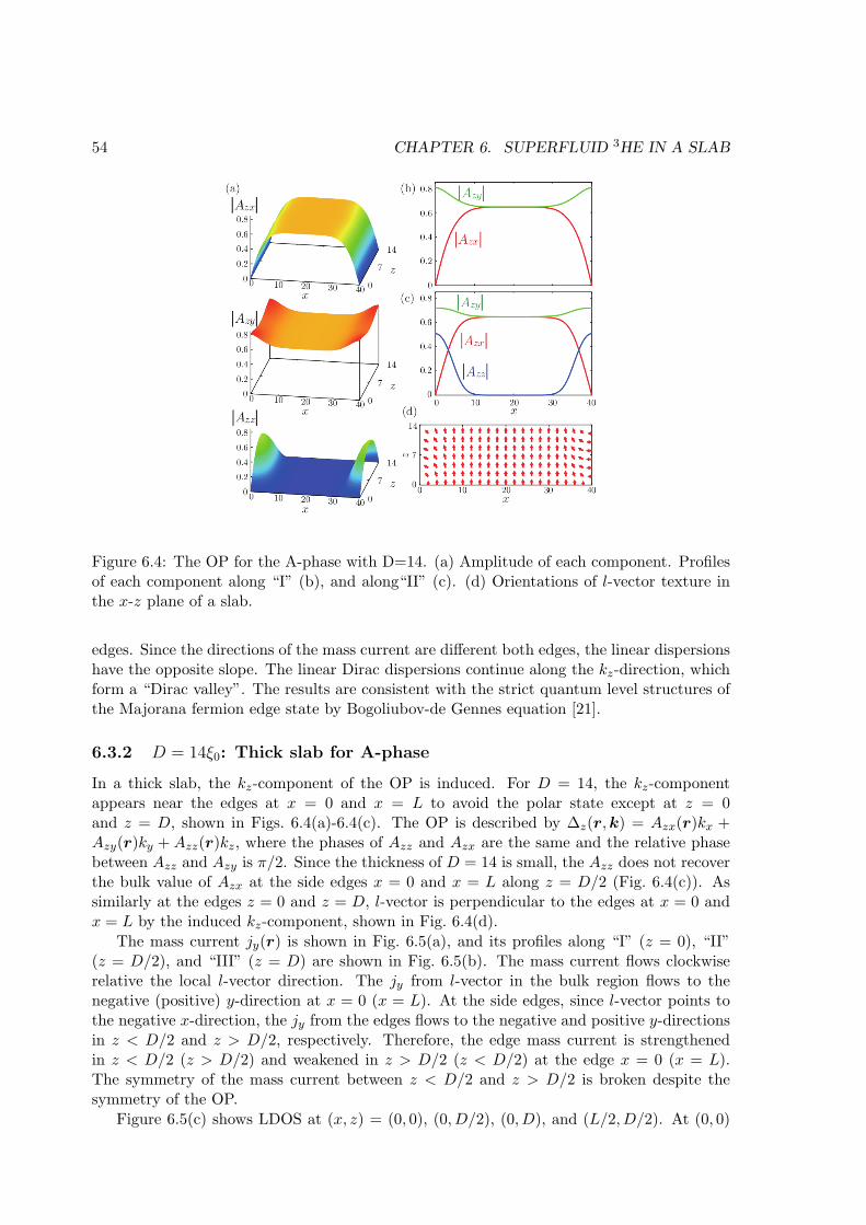
54 CHAPTER 6. SUPERFLUID 3HE IN A SLAB
Figure 6.4: The OP for the A-phase with D=14. (a) Amplitude of each component. Profilesof each component along “I” (b), and along“II” (c). (d) Orientations of l-vector texture inthe x-z plane of a slab.
edges. Since the directions of the mass current are different both edges, the linear dispersionshave the opposite slope. The linear Dirac dispersions continue along the kz-direction, whichform a “Dirac valley”. The results are consistent with the strict quantum level structures ofthe Majorana fermion edge state by Bogoliubov-de Gennes equation [21].
6.3.2 D = 14ξ0: Thick slab for A-phase
In a thick slab, the kz-component of the OP is induced. For D = 14, the kz-componentappears near the edges at x = 0 and x = L to avoid the polar state except at z = 0and z = D, shown in Figs. 6.4(a)-6.4(c). The OP is described by ∆z(r,k) = Azx(r)kx +Azy(r)ky + Azz(r)kz, where the phases of Azz and Azx are the same and the relative phasebetween Azz and Azy is π/2. Since the thickness of D = 14 is small, the Azz does not recoverthe bulk value of Azx at the side edges x = 0 and x = L along z = D/2 (Fig. 6.4(c)). Assimilarly at the edges z = 0 and z = D, l-vector is perpendicular to the edges at x = 0 andx = L by the induced kz-component, shown in Fig. 6.4(d).
The mass current jy(r) is shown in Fig. 6.5(a), and its profiles along “I” (z = 0), “II”(z = D/2), and “III” (z = D) are shown in Fig. 6.5(b). The mass current flows clockwiserelative the local l-vector direction. The jy from l-vector in the bulk region flows to thenegative (positive) y-direction at x = 0 (x = L). At the side edges, since l-vector points tothe negative x-direction, the jy from the edges flows to the negative and positive y-directionsin z < D/2 and z > D/2, respectively. Therefore, the edge mass current is strengthenedin z < D/2 (z > D/2) and weakened in z > D/2 (z < D/2) at the edge x = 0 (x = L).The symmetry of the mass current between z < D/2 and z > D/2 is broken despite thesymmetry of the OP.
Figure 6.5(c) shows LDOS at (x, z) = (0, 0), (0, D/2), (0, D), and (L/2, D/2). At (0, 0)

6.3. A-PHASE 55
Figure 6.5: Calculated results for the A-phase with D=14. (a) Mass current jy(r) in thex-z plane. (b) Profiles of the mass current jy(r) along paths “I”, “II”, and “III”. (c) LDOSN(E, r) at “1”, “2”, “3”, and “5”. (d) Zero energy LDOS N(E = 0, r) along “I”, “II”, and“III”. Angle-resolved LDOS N(E, r, θ) with φ = 0 at “1” (e), “2” (f), and “3” (g). (h) Thepeak energy of angle-resolved LDOS as a function of kz for ky = 0 at “1”.
and (0, D) (the lines “1” and “3”), there are the zero energy LDOS and a small peak at alow energy indicated by the arrow in Fig. 6.5(c). Although l-vector points to the edge, thezero energy LDOS also exists at (0, D/2) (the line “2”). The lines “1” and “3” are slightlydecreased and increased, respectively, in low energy from the small peak as energy increases.The line “2” is almost constant in low energy. The LDOS (the lines “1”, “2”, and “3”) areenhanced sharply near E ≈ 0.5. The LDOS at (L/2, D/2) (the line “5”) shows the typicalspectral behavior of the point node. In Fig. 6.5(d) we show the extent of the zero energyedge mode toward the bulk from the edge at x = 0. The amounts of the zero energy LDOSat x = 0 along z = D/2 and z = D (the lines “II” and “III”) are smaller than that alongz = 0 (the line “I”). The extent of the zero energy LDOS along “III” is of the order of 5ξ0 asin the thin slab D = 8; however, the zero energy LDOS along “I” and “II” are more widelyextended.
The angle-resolved LDOS N(E, r, θ) with φ = 0 at (0, 0), (0, D/2), and (0, D) are,respectively, displayed in Figs. 6.5(e), 6.5(f), and 6.5(g). The zero energy peaks of the angle-resolved LDOS appear except for θ = 0. The peaks of the line θ = 0 at the finite low energyappear from the upper and lower surfaces because the kz-component of the pair potentialis non-vanishing. Since thickness D = 14 is small, the original zero energy peak of θ = 0
perpendicular to the upper and lower surfaces is split into the finite energy peaks, which isdiscussed particularly for the B-phase in next section. The splitting peaks at (0, 0) are shownin Fig. 6.5(h) only at kz = ±1 for ky = 0. The finite energy peaks compose the small peak ofthe LDOS in the lines “1” and “3” in Fig. 6.5(c). Since the position (0, D/2) is apart formthe upper and lower surfaces, the energy peaks of θ = 0 are small. Consequently, the peakof the LDOS at low energy is not clear (the line “2” in Fig. 6.5(c)). The point nodes of theOP near the side edges have a tilt to the x-direction according to l-vector, or the anti-nodesof the OP lie to some angles from the kz-axis. Thus, the incident QPs from (0, 0) with lowangles from the kz-axis do not feel the clear small gap in the vicinity of the point nodes. Forinstance, the line θ = 30 in Fig. 6.5(e) should be compared with that in Fig. 6.3(e) for thethin slab D = 8. Therefore, the gap-like LDOS enhanced sharply near E ≈ 0.5 appears (theline “1” in Fig. 6.5(c)). On the other hand, the incident QPs from (0, D) with low angles

56 CHAPTER 6. SUPERFLUID 3HE IN A SLAB
from the kz-axis are reflected at the edge and regarded as with low angles from the −kz-axis.Since the QPs feel the small gap in the vicinity of the point nodes, they have the clear peaksin the angle-resolved LDOS (Fig. 6.5(g)). Therefore, the LDOS is slightly increased in lowenergy as energy increases (the line “3” in Fig. 6.5(c)). Since the QPs at (0, D/2) have thetwo kinds of the characteristic momentum, the LDOS is almost constant in low energy (theline “2” in Fig. 6.5(c)).
The LDOS at the side edge is different and depends on the thickness of the slab. In thethin slab (D = 8), l-vector points to the z-direction everywhere and the LDOS is N(E) =N(0) + αE2 in low energy. In contrast, in the thick slab (D = 14), l-vector points to thex-direction near the side edge and the LDOS is N(E) = N(0) +Ngap(E), where Ngap(E) isalmost zero in low energy and increases sharply near E ≈ 0.5 like the LDOS with the fullgap state. The edge mass current varies along the side edge in the thick slab, which is alsoa great difference with the thin slab.
Note that the A-phase is metastable in the slab with D = 14 at T = 0.2Tc in the weak-coupling limit for P → 0 [106]. In the same slab, the A-phase is stabilized at T = 0.9Tc [106];however, l-vector points to only the z-direction, because the kz-component is absent owingto the longer coherence length at higher temperature. The mechanism is similar to that theA-phase is more stable than the B-phase, which has the kx-, ky-, and kz-components, in athin slab at low temperature. The calculated results shown in this subsection is not in freeenergy minimum at P = 0; however, the strong-coupling effect by pressure stabilizes theA-phase texture. Thus, the above characteristics from the texture will be observed at finitepressure.
6.4 B-phase
The B-phase is stable when the thickness of a slab is larger than ≈ 13ξ0 at T = 0.2Tc [106].The OP of the B-phase is described by [2]
Aµi = Rµi(nd, θd)
Axx 0 00 Ayy 00 0 Azz
,
where Rµi(nd, θd) is a rotation matrix with a rotation axis nd and a rotation angle θd aboutnd. The rotation matrix gives the relative angle between the orbital momentum and thedirection along which the spin of a Cooper pair is zero. The spin state is stable by thedipole-dipole interaction when θd = θL ≡ cos−1(−1/4) and nd is perpendicular to the surfacein the absence of a magnetic field [2]. If the thickness of a slab is much smaller than thedipole coherence length, nd is locked to the z-axis. Thus, we derive Axx(r), Ayy(r), andAzz(r) with the uniform rotation matrix R(z, θL). Note that the three components have thesame phase.
At the surface of a slab, since the normal component to the surface of the orbital statevanishes, the planar state will be realized. The OP in the planar state is described by [2]
Aµi = Rµi(nd, θd)
Axx 0 00 Ayy 00 0 0
,
where we regard the z-axis as perpendicular to the edge. If θd = 0, the OP can be written

6.4. B-PHASE 57
Figure 6.6: The OP for the B-phase with D=30. (a) Amplitude of each component. Profilesof each component along “I” (b), and along“II” (c).
by other descriptions as
∆↑↑(k) = −∆p(kx − iky), ∆↓↓(k) = ∆p(kx + iky),
where ∆↑↑ = −∆x + i∆y, ∆↓↓ = ∆x + i∆y, and ∆p = Axx = Ayy. Therefore, in the planarstate, Sz = +1 spin state has Lz = −1 orbital angular momentum and Sz = −1 spin statehas Lz = +1 orbital angular momentum.
6.4.1 D = 30ξ0: Thick slab for B-phase
We consider that the thickness of a slab is much longer than the coherence length, namely,the thickness can be regarded as macroscopic for the OP, and much shorter than the dipolecoherence length. The requirement is satisfied for a thickness of D = 30. It is clearly seenthat the component of the OP perpendicular to the edge becomes zero in Fig. 6.6(a). Thepolar state ky occurs at the corner “1” (x = 0, z = 0). The planar state kx − iky for theup-up spin Cooper pairs and kx + iky for the down-down spin Cooper pairs is attained in themiddle region around “4” (x = L/2, z = 0), shown in Fig. 6.6(b). The planar state ky ± ikz
is realized at the side edge “2” (x = 0, z = D/2) and the OP is recovered to the bulk valueof the B-phase around “5” (x = L/2, z = D/2), shown in Fig. 6.6(c). At all edges (x = 0,x = L, z = 0, and z = D), the Majorana fermion edge state exists [65, 66, 68].
The spin current jxsy(r), jz
sy(r), jysx(r), and jy
sz(r) are shown in Fig. 6.7(a). Since thespin current flows in the three-dimensional real space, we show the schematic flow of thespin current in Fig. 6.7(b). The spin current for the i-component of spin turns around thei-axis. This is understandable as follows: Since the up-up spin Cooper pairs have negativechirality and the down-down spin Cooper pairs have positive chirality, the z-component ofthe spin current turns around the z-axis. Other components are also understood in the samemanner. Note that the schematic flow in Fig. 6.7(b) is derived from Aii before rotation by

58 CHAPTER 6. SUPERFLUID 3HE IN A SLAB
Figure 6.7: (a) The spin current for the B-phase with D = 30. The unit of the spin currentis 10−9 J/m2. (b) A schematic flow of the spin current for Sx, Sy, and Sz components.
R(z, θL). The rotation axes for the x- and y-component of the spin current are changedcorrespondingly.
Figure 6.8(a) shows the LDOS. It is seen that only the line “1” (x = 0, z = 0) hasthe zero energy LDOS from the zero energy Andreev bound state of QPs without the ky-component. The lines “2” and “4” (x = 0, z = D/2 and x = L/2, z = 0) are almost the sameand show the linear relation N(E, r) ∝ E near E = 0 which reflects the surface Andreevbound states [108, 109]. The line “5” (x = L/2, z = D/2) corresponds to the bulk LDOSwhere the full gap is expected. In Fig. 6.8(b) we show the extension of the zero energy statetoward the middle from the edge at x = 0. The zero energy LDOS of the line “I” (z = 0)reduces sharply as approaching the middle region from the edge. It is found that the valueN(E = 0, x = 0) in the line “IV” (z = 0.5) is much smaller than that of the line “I”. Theline “II” along z = D/2 shows the absence of the zero energy LDOS. Therefore, we concludethat the zero energy LDOS is localized at the corner of the order of ξ0. The peak energy ofthe angle-resolved LDOS is shown in Figs. 6.8(c) for the side edge and 6.8(d) for the lowersurface. Figure 6.8(c) is as a function of ky for kz = 0 and as a function of kz for ky = 0 at“2” (x = 0, z = D/2). Figure 6.8(d) is as a function of kx for ky = 0 and as a function of ky
for kx = 0 at “4” (x = L/2, z = 0). These show that the side edge and lower surface havethe same dispersion relation for low energy. The linear dispersion forms the Majorana coneat the surface [65].
The peak energy of the angle-resolved LDOS at the corner (0, 0) is shown in Figs. 6.8(e)and 6.8(f). The energy is dispersionless along the kz- and kx-axes for ky = 0. The Diracvalley-type dispersion is composed of the zero energy LDOS at the corner (the line “1” in

6.4. B-PHASE 59
N(E
, r)
E
(a)
(c)
(b)
E
(d)
1
2
5
4
0
1
2
3
4
5
0 0.2 0.4 0.6 0.8 1 0
0.1
0.2
0.3
0.4
0.5
0.6
0.7
0 10 20
N(E
=0,
r)
x
I
IVII
-1
-0.5
0
0.5
1
kxky
E
-1
-0.5
0
0.5
1
kykz
-1 -0.5 0 0.5 1
E
ki
ky
kz
-1
-0.5
0
0.5
1
-1 -0.5 0 0.5 1
E
ki
kx
ky
-1
-0.5
0
0.5
1(e) (f)
Figure 6.8: The LDOS for the B-phase with D = 30. (a) LDOS N(E, r) at “1”, “2”, “4”,and “5”. (b) Zero energy LDOS N(E = 0, r) along “I”, “II”, and “IV” (z = 0.5). The peakenergy of angle-resolved LDOS as a function of ky for kz = 0 and as a function of kz forky = 0 at “2” (c), and as a function of kx for ky = 0 and as a function of ky for kx = 0 at“4” (d). (e) and (f) are the same plots as (c) and (d), but at “1”.
Fig. 6.8(a)). This is different from the Majorana cone at the surface.
6.4.2 D = 14ξ0: Thin slab for B-phase
We consider D = 14 in thickness of a slab which is the critical thickness for stabilizing theB-phase below which the stripe phase becomes stable [106]. Since the thickness is short,the kz-component of the OP can not completely recover the bulk value. Except that thekz-component is reduced, the qualitative features of the OP and the spin current are thesame in the case of D = 30; however, the LDOS shows different spectrum.
Figure 6.9 shows the LDOS and the peak energy of the angle-resolved LDOS, whichare compared with those in Fig. 6.8. The differences between them are following: Since thethickness of the slab is short, the line “5” for the center (x = L/2, z = D/2) has the spectrumfrom the full gap and the linear relation near E = 0, shown in Fig. 6.9(a). The latter comesfrom the contributions extending from the upper and lower surfaces. The line “2” for theside edge (x = 0, z = D/2) in Fig. 6.9(a) has the small peak at E ≈ 0.35 composed of thedeformed Majorana cone in 0.5 / |kz| / 0.7, shown in Fig. 6.9(c), because the QPs with thekz-component reflect that the kz-component of the OP does not recover the bulk value. Thepeak energy at “4” for the lower surface in Fig. 6.9(d) implies that the lowest energy of theMajorana cone is lifted from zero because of the tunneling of the zero energy modes boundat two surfaces corresponding to the upper and lower surfaces. For the same reason, the zeroenergy modes at the corner is split for kz = ±1 in Fig. 6.9(e) and for ky = 0 or kx = 0 in
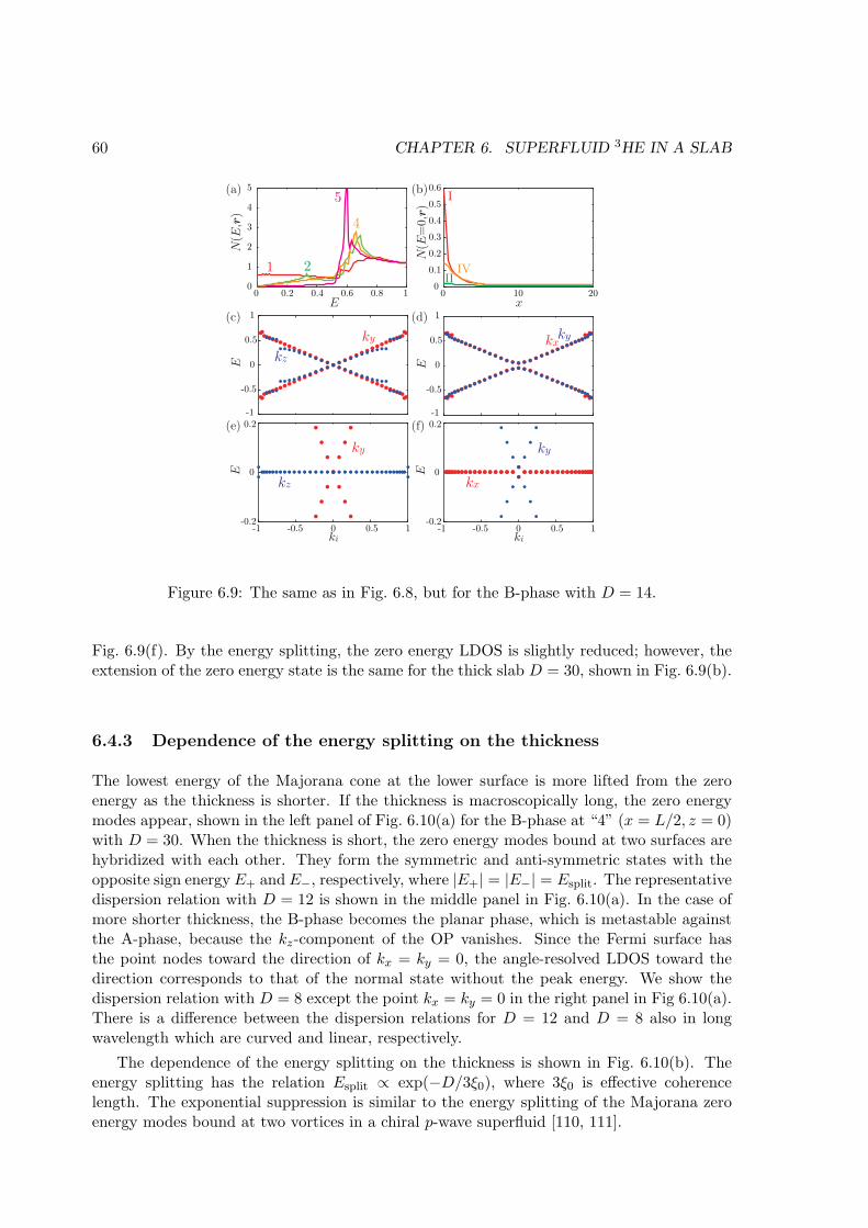
60 CHAPTER 6. SUPERFLUID 3HE IN A SLAB
0
1
2
3
4
5
0 0.2 0.4 0.6 0.8 1
-1
-0.5
0
0.5
1
kxky
N(E
, r)
E
(a)
(c)
(b)
E
(d)
1 2
5
4
0
0.1
0.2
0.3
0.4
0.5
0.6
0 10 20
N(E
=0, r
)
x
I
IVII
-1
-0.5
0
0.5
1
E
ky
kz
-0.2
0
0.2
-1 -0.5 0 0.5 1
E
ki
ky
kz
-0.2
0
0.2
-1 -0.5 0 0.5 1
E
ki
kx
ky
(e) (f)
Figure 6.9: The same as in Fig. 6.8, but for the B-phase with D = 14.
Fig. 6.9(f). By the energy splitting, the zero energy LDOS is slightly reduced; however, theextension of the zero energy state is the same for the thick slab D = 30, shown in Fig. 6.9(b).
6.4.3 Dependence of the energy splitting on the thickness
The lowest energy of the Majorana cone at the lower surface is more lifted from the zeroenergy as the thickness is shorter. If the thickness is macroscopically long, the zero energymodes appear, shown in the left panel of Fig. 6.10(a) for the B-phase at “4” (x = L/2, z = 0)with D = 30. When the thickness is short, the zero energy modes bound at two surfaces arehybridized with each other. They form the symmetric and anti-symmetric states with theopposite sign energy E+ and E−, respectively, where |E+| = |E−| = Esplit. The representativedispersion relation with D = 12 is shown in the middle panel in Fig. 6.10(a). In the case ofmore shorter thickness, the B-phase becomes the planar phase, which is metastable againstthe A-phase, because the kz-component of the OP vanishes. Since the Fermi surface hasthe point nodes toward the direction of kx = ky = 0, the angle-resolved LDOS toward thedirection corresponds to that of the normal state without the peak energy. We show thedispersion relation with D = 8 except the point kx = ky = 0 in the right panel in Fig 6.10(a).There is a difference between the dispersion relations for D = 12 and D = 8 also in longwavelength which are curved and linear, respectively.
The dependence of the energy splitting on the thickness is shown in Fig. 6.10(b). Theenergy splitting has the relation Esplit ∝ exp(−D/3ξ0), where 3ξ0 is effective coherencelength. The exponential suppression is similar to the energy splitting of the Majorana zeroenergy modes bound at two vortices in a chiral p-wave superfluid [110, 111].
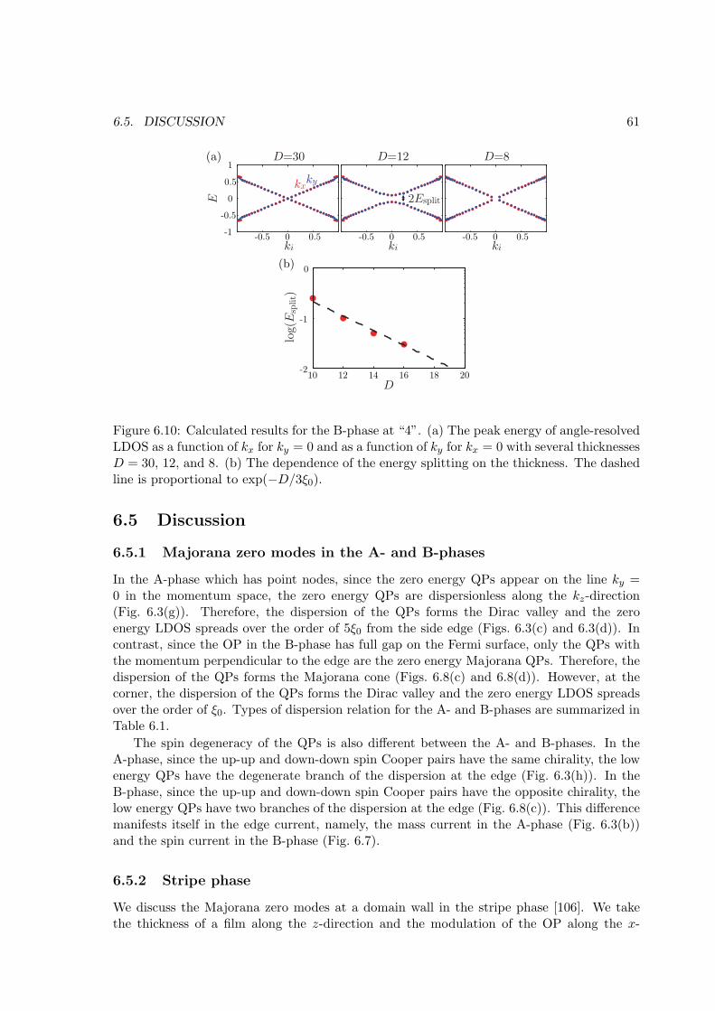
6.5. DISCUSSION 61
-1
-0.5
0
0.5
1
-0.5 0 0.5
E
ki
kxky
-0.5 0 0.5 -0.5 0 0.5
2Esplit
D=30 D=12 D=8
kiki
-2
-1
0
10 12 14 16 18 20D
log(
Esp
lit)
(a)
(b)
Figure 6.10: Calculated results for the B-phase at “4”. (a) The peak energy of angle-resolvedLDOS as a function of kx for ky = 0 and as a function of ky for kx = 0 with several thicknessesD = 30, 12, and 8. (b) The dependence of the energy splitting on the thickness. The dashedline is proportional to exp(−D/3ξ0).
6.5 Discussion
6.5.1 Majorana zero modes in the A- and B-phases
In the A-phase which has point nodes, since the zero energy QPs appear on the line ky =0 in the momentum space, the zero energy QPs are dispersionless along the kz-direction(Fig. 6.3(g)). Therefore, the dispersion of the QPs forms the Dirac valley and the zeroenergy LDOS spreads over the order of 5ξ0 from the side edge (Figs. 6.3(c) and 6.3(d)). Incontrast, since the OP in the B-phase has full gap on the Fermi surface, only the QPs withthe momentum perpendicular to the edge are the zero energy Majorana QPs. Therefore, thedispersion of the QPs forms the Majorana cone (Figs. 6.8(c) and 6.8(d)). However, at thecorner, the dispersion of the QPs forms the Dirac valley and the zero energy LDOS spreadsover the order of ξ0. Types of dispersion relation for the A- and B-phases are summarized inTable 6.1.
The spin degeneracy of the QPs is also different between the A- and B-phases. In theA-phase, since the up-up and down-down spin Cooper pairs have the same chirality, the lowenergy QPs have the degenerate branch of the dispersion at the edge (Fig. 6.3(h)). In theB-phase, since the up-up and down-down spin Cooper pairs have the opposite chirality, thelow energy QPs have two branches of the dispersion at the edge (Fig. 6.8(c)). This differencemanifests itself in the edge current, namely, the mass current in the A-phase (Fig. 6.3(b))and the spin current in the B-phase (Fig. 6.7).
6.5.2 Stripe phase
We discuss the Majorana zero modes at a domain wall in the stripe phase [106]. We takethe thickness of a film along the z-direction and the modulation of the OP along the x-

62 CHAPTER 6. SUPERFLUID 3HE IN A SLAB
Table 6.1: Types of dispersion relation at the upper or lower surface, side edge, and cornerof a slab for the A- and B-phases. Dirac valley is formed from linear dispersion from E = 0along a certain momentum direction and dispersionless zero energy modes along anothermomentum direction in long wavelength. Majorana cone is formed from isotropic linerdispersion from E = 0 on the plane parallel to a surface in the momentum space in longwavelength, where the zero mode is in a point on the Fermi surface. The mark × indicatesabsence of zero energy modes.
upper or lower surface side edge cornerA-phase thin slab (D = 8ξ0) × Dirac valley Dirac valley
thick slab (D = 14ξ0) × Dirac valley Dirac valleyB-phase thin slab (D = 14ξ0) × Majorana cone Dirac valley
thick slab (D = 30ξ0) Majorana cone Majorana cone Dirac valley
direction. In the stripe phase, the kz-component of the OP changes the sign at the domainwall perpendicular to the x-direction so that the pair breaking by the reflection at the surfaceof the film is prevented. Then, the OP is described as ∆right = (∆‖kx,∆‖ky,∆⊥kz) to theright of the domain wall and ∆left = (∆‖kx,∆‖ky,−∆⊥kz) to the left of the domain wall,where ∆‖ is finite everywhere and ∆⊥ vanishes at the domain wall.
The QPs with the kz-component which across the domain wall have the finite energyAndreev bound states because they feel the sign change of the kz-component of the pairpotential, which is not the exact π-phase shift. In addition, since the QPs with kz = 0feel the full gap of the pair potential, they are not excited in low energy. Therefore, theMajorana zero energy QP is absent at the domain wall in the stripe phase. The domain wallis qualitatively different from the edge.
6.5.3 Experimental proposal
There are several experimental means to detect the Majorana nature. Surface specific heatmeasurement, which was performed in connection with detection of the Andreev surfacebound state [112], resolves the side edge contribution Csurface(T ) = γT of the A-phase ina thin slab at low temperatures, where γ ∝ N(E = 0), because the bulk contributionCbulk ∝ T 3 which comes from point nodes where N(E) ∝ E2 is distinguishable. Note that,in the A-phase, the contribution from the two upper and lower specular surfaces in the slabgeometry is the same as that from the bulk. Thus, the surface specific heat Csurface(T ) = γTof the Majorana QPs is distinctive. If the l-vector direction is modulated near the side edge,the LDOS at the surface is N(E) = N(0) + Ngap(E). The surface specific heat from theLDOS is also Csurface(T ) = γT .
In the B-phase, the zero energy LDOS is localized at the corner of the order of ξ0. Thecontribution from the corner is interesting but smaller than that of the surface. Since wewill discriminate Cbulk ∝ T−3/2e−∆/kBT from the gap ∆ and Csurface ∝ T 2 from the linearbehavior of LDOS N(E, r) ∝ E near E = 0, the Majorana fermion can be observed. Inthe slab with short thickness where the zero energy modes are split at the upper and lowersurfaces, the difference of the specific heat from the surface and bulk will not be distinctivebecause the gap structure and linear behavior of the LDOS coexist.
The observation of the edge mass current in the A-phase, which is intimately connected
6.6. SUMMARY 63
with the intrinsic angular momentum [2], is also hopeful. The magnitude of the edge masscurrent is unchanged in wider slabs than L = 40ξ0 for which we have calculated. Consideringthe observation of the torque from the edge mass current for a 10 mm × 7 mm × 0.6 µm slabsample (Bennett et al. [100] had been used) by a typical torsional oscillator, the frequencyshift from the edge mass current is of the order of 10−23 Hz [113]. The torque is too smallto observe by a torsional oscillator because the magnitude is ∼ N~/2, where N is the totalnumber of 3He atoms in the slab sample. We have to consider other experimental methods.Analytical derivation of the torque is shown in Appendix B. Also the edge spin current in theB-phase which flows three-dimensionally has been obtained quantitatively. The techniquesto detect the spin current is desired. The specific experimental proposal to observe the edgecurrent is a future problem.
The most direct evidence of the Majorana nature is derived from the observation of theanisotropic spin susceptibility. If we use the Majorana nature of the edge state, in the A-phase, the local spin operators result in Sx ≈ Sy ≈ 0 and only Sz parallel to d-vector remainsnontrivial for T Tc [64]. This predicts the Ising-like spin dynamics for the local spinoperator parallel to d-vector in the A-phase as well as that perpendicular to the edge in theB-phase [65, 68]. This is in sharp contrast to the susceptibility parallel to d-vector in the bulkA-phase which is suppressed at low temperatures according to the Yosida function. On theother hand, the susceptibility perpendicular to d-vector still assumes the bulk value, whichis the same as it in the normal state. The anisotropic susceptibility has been discussed alsoby Shindou et al. [114] and has been calculated in the B-phase by Nagato et al. [68].
QP scattering or QP beam experiments are extremely interesting. They were performedin the past on 4He where roton-roton scattering is treated [115] and on the 3He B-phasewhere the surface Andreev bound state is investigated [116, 117]. Using this method, wemay pick up Majorana QPs with a particular wave number. Particularly in the A-phase, theMajorana QPs from the edge is separated from other QPs from the nodal region.
Another option might be to use a free surface where the Majorana fermion surface stateis formed. As shown by Kono [118], it can be detected through the excitation modes of thefloating Wigner lattice of electrons placed on the surface. We need a special, but feasibleconfiguration of the experimental setups.
Note that the recent work of transverse acoustic impedance measurements to detect thesurface bound states in the superfluid 3He will derive the important information of theMajorana QPs [119, 120, 121].
6.6 Summary
We have designed a concrete experimental setup to observe the Majorana nature at the surfacein the slab geometry. In connection with realistic slab samples, we have considered the upperand lower surfaces and the side edges including the corners with several thicknesses. We havedemonstrated that the quasi-classical Eilenberger equation yields the quantitatively reliableinformation on physical quantities for the superfluid 3He A- and B-phases. Specifically, wehave exhibited the difference of LDOS between the A- and B-phases and evaluated the masscurrent for the A-phase and the spin current for the B-phase quantitatively. Then, we haveshown the influence on the Majorana zero modes from the spatial variation of l-vector for theA-phase in the thick slab and the energy splitting of the zero energy modes for the B-phaseconfined in the thin slabs. The corner of the slab in the B-phase is accompanied by theunique zero energy LDOS of corner modes. In addition, we have demonstrated the absence
64 CHAPTER 6. SUPERFLUID 3HE IN A SLAB
of the Majorana zero energy QP at the domain wall in the stripe phase. On the basis of thequantitative consequences, it is proposed that the measurement of the specific heat, the edgecurrent, and the anisotropic spin susceptibility provides feasible and verifiable experimentsto check the Majorana nature. The control on the thickness of the slab is crucial to detectthe Majorana surface states. The experiment controlling the thickness of the film of thesuperfluid 3He is interesting [101].

Chapter 7
p-wave resonant superfluids ofFermi atomic gases
Recently, p-wave resonant superfluidity attracts much attention in Fermionic alkaline atomicgases, such as 6Li [13, 14, 15] and 40K [16, 17, 18], both experimentally and theoretically [50,122, 123, 124, 125]. Experiments into achieving p-wave resonant superfluidity are steadilyprogressing and hence it is timely and necessary to consider the generic properties of p-wavesuperfluidity both at rest and under rotation to detect its superfluidity, which is signifiedby non-trivial topological structures or vortices. In this chapter, textures and vortices forp-wave resonant superfluids of Fermi atomic gases are calculated by the Ginzburg-Landau(GL) theory.
The textures are different from the superfluid 3He by the boundary condition, becauseFermi atomic gases are confined in harmonic trap potential. The trap potential is easilycontrolled, resulting in various shapes, such as cigar or pancake shapes. As we describebelow, the trapping potential can be an important tool to control the three-dimensional (3D)texture. Indeed, the 3D trapping structure constrains the possible textures. Our purpose isto investigate a possible 3D textures in a 3D harmonic trap potential and thereby to helpidentifying p-wave superfluidity.
Moreover, we investigate vortices with Majorana quasi-particle (QP) in “spinless” p-waveresonant superfluids of Fermi atomic gases with high controllability [126, 63]. Therefore, theywill be a favorable platform of quantum computation.
The organization of this chapter is as follows: We employ the GL framework underrotation and trap potential which relies only on global symmetry principle. The GL freeenergy functional form is introduced and the relevant physical quantities, such as supercurrentand l-vector are given in Sec. 7.1. We show the phase diagram of the stable states for uniformand infinite system, and explain how to numerically examine realistic confined systems inSec. 7.2. Section 7.3 presents the stable texture in the cigar shape trap, especially, we mentionthe spontaneous supercurrent at rest and the half-quantum vortex (HQV) under rotation.In Sec. 7.4, we show the different textures stabilized in the pancake shape. In Sec. 7.5, weconsider the quasi-two-dimensional (quasi-2D) shape trap. In this trap, a singular vortexwith Majorana QP is realized. The final section is devoted to a summary.
65

66 CHAPTER 7. P -WAVE RESONANT SUPERFLUIDS OF FERMI ATOMIC GASES
7.1 Formulation
Here we employ the GL framework [2]. This framework is general and flexible enough toallow us to examine a generic topological structure, and applicable to cold fermionic atomgases with a harmonic trap potential under kBTc ~ω, where Tc and ω are the transitiontemperature and the trap frequency, respectively [127]. In terms of the tensor Aµi formingorder parameter (OP) of p-wave pairing the most general GL functional density fbulk for thebulk condensation energy up to quartic order is described as
fbulk = −αiA∗µiAµi + β1A
∗µiA
∗µiAνjAνj + β2A
∗µiAµiA
∗νjAνj+β3A
∗µiA
∗νiAµjAνj
+β4A∗µiAνiA
∗νjAµj+β5A
∗µiAνiAνjA
∗µj , (7.1)
which is invariant under spin and real space rotations in addition to the gauge invarianceU(1)×SO(S)(3)×SO(L)(3). The quartic order terms are characterized by five independentinvariants, β1–β5 in general [2]. Since the spin degrees of freedom are frozen due to appliedmagnetic field for magnetic Feshbach resonance, only the orbital degrees of freedom Ai inAµi = (m + in)µAi are active, where m and n are orthogonal. Namely it reduces to
fbulk = −α0(1 − ti)A∗iAi + β24A
∗iAiA
∗jAj + β3A
∗iA
∗iAjAj , (7.2)
where β24 = β2 + β4 and ti = T/Tci (Tci is the transition temperature for the i-component).As mentioned in Chap. 3, the dipole-dipole interaction causes splitting of the transitiontemperatures into two groups Tcx = Tcy and Tcz. We introduce α = Tcx/Tcz, which indicatesthe degree of the broken symmetry of the system and characterizes atomic species used [17].The pairing state having the orbital projection ml = 0 is favorable over ml = ±1, namely0 < α < 1 due to the dipole-dipole interaction [17]. The three components become degeneratefor α→ 1. When α→ 0, the polar state with the OP ∆(k) = Azkz tends to be stable.
The gradient energy consisting of the three independent terms [2] is given by
fgrad = K1(∂∗i A∗j )(∂iAj) +K2(∂∗i A
∗j )(∂jAi) +K3(∂∗i A
∗i )(∂jAj). (7.3)
The centrifugal potential energy due to rotation with Ω, which is derived in Appendix C, iswritten as
fcent = −m2
~2Ω2ρ2(K1A
∗iAi +K2|Aθ|2 +K3|Aθ|2), (7.4)
where ∂i = ∇i − i(m/~)(Ω × r)i. For Ω ‖ z, ρ2 = x2 + y2 and Aθ = −Ax sin θ + Ay cos θ inthe cylindrical coordinates.
The GL parameters α0, β24 = β2 + β4, β3 and K1 = K2 = K3 = K are estimated bytaking the weak-coupling approximation [2]:
α0 =N(0)
3, β2 = β3 = β4 =
7ζ(3)N(0)120(πkBTc)2
≡ β (7.5)
and
K =7ζ(3)N(0)(~vF )2
240(πkBTc)2(7.6)
where N(0) is the density of states at the Fermi level and vF is the Fermi velocity. The weak-coupling approximation should be a good guide for understanding the generic properties ofthe p-wave superfluids of atom gases because it has been applied successfully, even to liquid3He with strong interacting fermions and only small additional strong corrections [2].
7.1. FORMULATION 67
The GL free energy density functionals, eqs. (7.2)–(7.4), can be expressed with di-mensionless units. The units of OP, length, and rotation frequency are the OP ampli-tude of the chiral state in a bulk ∆0 =
√10π2/7ζ(3)kBTc, the GL coherence length ξ0 =√
7ζ(3)/48π2(~vF /kBTc) with zero temperature, and Ω0 = ~/mξ20 , respectively, where vF isthe Fermi velocity. In the dimensionless unit, eqs. (7.2)–(7.4) are written as
fbulk = − (1 − ti)A∗iAi +
12A∗
iAiA∗jAj +
14A∗
iA∗iAjAj , (7.7)
fgrad =35[(∂∗i A
∗j )(∂iAj) + (∂∗i A
∗j )(∂jAi) + (∂∗i A
∗i )(∂jAj)
], (7.8)
fcent = − 35Ω2ρ2(A∗
iAi + 2|Aθ|2), (7.9)
respectively, where ∂i = ∇i − i(Ω× r)i. From now on we use the dimensionless expressions.The effect of harmonic trap potential on condensates depends on the dimensionless pairing
interaction Γ that determines the transition temperature Tc = CEF exp(−1/Γ), where EF
is the Fermi energy and C is a numerical coefficient of order unity [127]. We use the unit~ω0 =
√144π2/35ζ(3)
√2Γ/(1 + 2Γ)kBTc for the trap frequency ω. The p-wave triplet paring
interaction is Γ ≈ λ2/13 with a gaseous parameter λ = 2|a|pF /π~, where a is the scatteringlength and pF is the Fermi momentum [128]. The harmonic trap potential term [127] is
fharm =35ω2⊥(ρ2 + λ2z2)A∗
iAi, (7.10)
where the dimensionless radial confining potential is ω⊥ and the anisotropy of the harmonictrap is expressed as λ ≡ ωz/ω⊥. The harmonic trap potential term acts to lower the transitiontemperatures.
Rotation frequency is also normalized by the critical rotation frequency Ωc, where con-densates fly away from the trap potential by centrifugal force. We sum up the centrifugalenergy and the trap potential energy as
fcent + fharm =35(ω2
⊥ − Ω2)ρ2(|Ar|2 + |Az|2) +35(ω2
⊥ − 3Ω2)ρ2|Aθ|2 +35λ2ω2
⊥z2A∗
iAi
with cylindrical coordinates. Therefore, the critical rotation frequency is given by Ωc =ω⊥/
√3.
The relevant physical quantities are described in terms of the OP Ai(r) as follows. Thetotal free energy:
F =∫d3r (fbulk + fgrad + fcent + fharm) . (7.11)
The current density:
ji(r) ≡ 2Im[A∗
j∇iAj +A∗j∇jAi +A∗
i∇jAj
]. (7.12)
l-vector:
li(r) ≡ −iεijkA∗
jAk
| ∆(r) |2(7.13)
with| ∆(r) |2= A∗
iAi. (7.14)
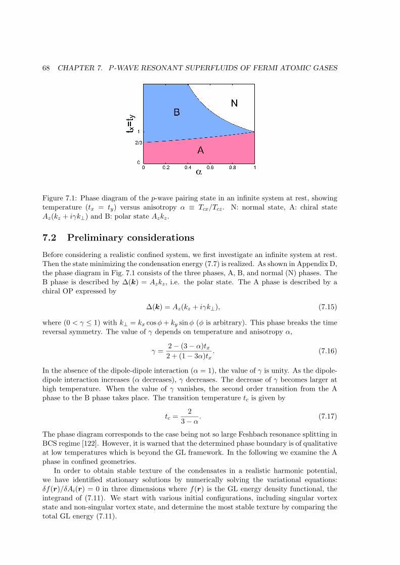
68 CHAPTER 7. P -WAVE RESONANT SUPERFLUIDS OF FERMI ATOMIC GASES
Figure 7.1: Phase diagram of the p-wave pairing state in an infinite system at rest, showingtemperature (tx = ty) versus anisotropy α ≡ Tcx/Tcz. N: normal state, A: chiral stateAz(kz + iγk⊥) and B: polar state Azkz.
7.2 Preliminary considerations
Before considering a realistic confined system, we first investigate an infinite system at rest.Then the state minimizing the condensation energy (7.7) is realized. As shown in Appendix D,the phase diagram in Fig. 7.1 consists of the three phases, A, B, and normal (N) phases. TheB phase is described by ∆(k) = Azkz, i.e. the polar state. The A phase is described by achiral OP expressed by
∆(k) = Az(kz + iγk⊥), (7.15)
where (0 < γ ≤ 1) with k⊥ = kx cosφ+ ky sinφ (φ is arbitrary). This phase breaks the timereversal symmetry. The value of γ depends on temperature and anisotropy α,
γ =2 − (3 − α)tx2 + (1 − 3α)tx
. (7.16)
In the absence of the dipole-dipole interaction (α = 1), the value of γ is unity. As the dipole-dipole interaction increases (α decreases), γ decreases. The decrease of γ becomes larger athigh temperature. When the value of γ vanishes, the second order transition from the Aphase to the B phase takes place. The transition temperature tc is given by
tc =2
3 − α. (7.17)
The phase diagram corresponds to the case being not so large Feshbach resonance splitting inBCS regime [122]. However, it is warned that the determined phase boundary is of qualitativeat low temperatures which is beyond the GL framework. In the following we examine the Aphase in confined geometries.
In order to obtain stable texture of the condensates in a realistic harmonic potential,we have identified stationary solutions by numerically solving the variational equations:δf(r)/δAi(r) = 0 in three dimensions where f(r) is the GL energy density functional, theintegrand of (7.11). We start with various initial configurations, including singular vortexstate and non-singular vortex state, and determine the most stable texture by comparing thetotal GL energy (7.11).
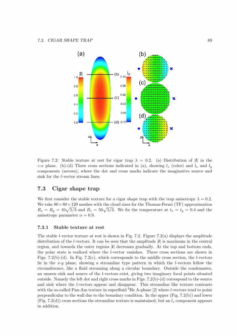
7.3. CIGAR SHAPE TRAP 69
Figure 7.2: Stable texture at rest for cigar trap λ = 0.2. (a) Distribution of |l| in thez-x plane. (b)-(d) Three cross sections indicated in (a), showing lz (color) and lx and lycomponents (arrows), where the dot and cross marks indicate the imaginative source andsink for the l-vector stream lines.
7.3 Cigar shape trap
We first consider the stable texture for a cigar shape trap with the trap anisotropy λ = 0.2.We take 80×80×120 meshes with the cloud sizes for the Thomas-Fermi (TF) approximationRx = Ry = 10
√5/3 and Rz = 50
√5/3. We fix the temperature at tx = ty = 0.4 and the
anisotropy parameter α = 0.9.
7.3.1 Stable texture at rest
The stable l-vector texture at rest is shown in Fig. 7.2. Figure 7.2(a) displays the amplitudedistribution of the l-vectors. It can be seen that the amplitude |l| is maximum in the centralregion, and towards the outer regions |l| decreases gradually. At the top and bottom ends,the polar state is realized where the l-vector vanishes. Three cross sections are shown inFigs. 7.2(b)-(d). In Fig. 7.2(c), which corresponds to the middle cross section, the l-vectorslie in the x-y plane, showing a streamline type pattern in which the l-vectors follow thecircumference, like a fluid streaming along a circular boundary. Outside the condensates,an unseen sink and source of the l-vectors exist, giving two imaginary focal points situatedoutside. Namely the left dot and right cross marks in Figs. 7.2(b)-(d) correspond to the sourceand sink where the l-vectors appear and disappear. This streamline like texture contrastswith the so-called Pan-Am texture in superfluid 3He A-phase [2] where l-vectors tend to pointperpendicular to the wall due to the boundary condition. In the upper (Fig. 7.2(b)) and lower(Fig. 7.2(d)) cross sections the streamline texture is maintained, but an lz component appearsin addition.

70 CHAPTER 7. P -WAVE RESONANT SUPERFLUIDS OF FERMI ATOMIC GASES
Figure 7.3: (a) Spontaneous circulating current flows at rest (Ω = 0) in the z-y plane alongthe z direction. Three cross sections indicated in the left figure, showing jz (color) and jxand jy components (arrows). (b)The current pattern under rotation (Ω = 0.3). It is seenthat the in-plane components jx and jy increase, producing the in-plane circular current dueto rotation.
The associated supercurrent structure is depicted in Fig. 7.3. The jz component showsa circulation supercurrent along the z-axis (see Fig. 7.3(a)). Since Ω = 0, this circulationsupercurrent is spontaneously generated. This non-trivial condensates flow can be explainedin supercurrent characteristic of chiral p-wave superfluid:
j = ρsvs + C(∇× l), (7.18)
where ρs and C are diagonal tensor coefficients. The supercurrent has a structure that issimilar to that for the total charge-current density of a system in classical electrodynamics.The current in classical electrodynamics is composed of two parts, the actual charge transportand an effective current in proportion to ∇× M due to the magnetization M generated bythe internal motion of the electrons. In chiral p-wave superfluid the Cooper pair may bethought of as representing the atom and l the magnetic orbital moment M . Therefore thefirst term in the supercurrent describes the usual flow of Cooper pairs, while the second oneis an “orbital” supercurrent driven by the spatial variation of l-vector.
In this system, the spontaneous supercurrent is not a usual supercurrent ρsvs but an“orbital” supercurrent C(∇ × l) with the trap potential. In the middle cross section inFig. 7.3(a), l-vector in-plane bending (∇× l)z produces a perpendicular current jz. However,at the upper and lower planes in Fig. 7.3(a), the supercurrent acquires the jx and jy com-ponents because of the non-vanishing lz component. Therefore, the perpendicular current atthe center bends such that the condensates are conserved. It is clear from Fig. 7.3(a) thatthe supercurrent circulates perpetually along the z direction parallel to the long axis of the

7.3. CIGAR SHAPE TRAP 71
Figure 7.4: (a) Texture change with rotational speed Ω relative to the in-plane trap frequencyω⊥. Middle cross sections are displayed showing lz (color) and lx and ly components (arrows).As Ω increases, l-vectors acquire a negative z component (seen as a color change). AtΩ = 0.4ω⊥ two plus HQVs enter from the y direction seen as yellow objects. At Ω = 0.5ω⊥four plus HQVs and two minus HQVs are present and the condensates expand and deform.(b) The enlarged figure of HQV where the local coordinates (r, θ) are shown.
trap. This result is non-trivial and a remarkable manifestation in the topological nature ofthe texture.
In Fig. 7.3(b) we also display the current patterns under rotation (Ω = 0.3ω⊥) for com-parison at rest. It is seen that the in-plane components jx and jy increase, producing thein-plane circular current due to rotation, in particular in the middle cross section. Thusunder rotations, the current consists of the spontaneous one along the z direction and theinduced circular current in the plane.
7.3.2 Half-quantum vortex under rotation
In Fig. 7.4 where we depict the middle cross sections of the stable solutions for variousrotation speeds (also see Fig. 7.6). It is seen that under rotation, the 3D texture deformscontinuously and smoothly. As the rotational speed increases, l-vectors in the x-y planepointing in the x direction acquire a negative z component, as seen by the color change fromgreen to blue. This deformation yields in plane circular “orbital” supercurrent as alreadyshown in Fig. 7.3(b).
Above a certain rotational speed (Ω = 0.4ω⊥), two HQVs enter from the y direction,where the l-vector at the core pointing in the positive z direction, as seen by the yellowobjects. The OP far away from the HQV core is described in terms of the local coordinated
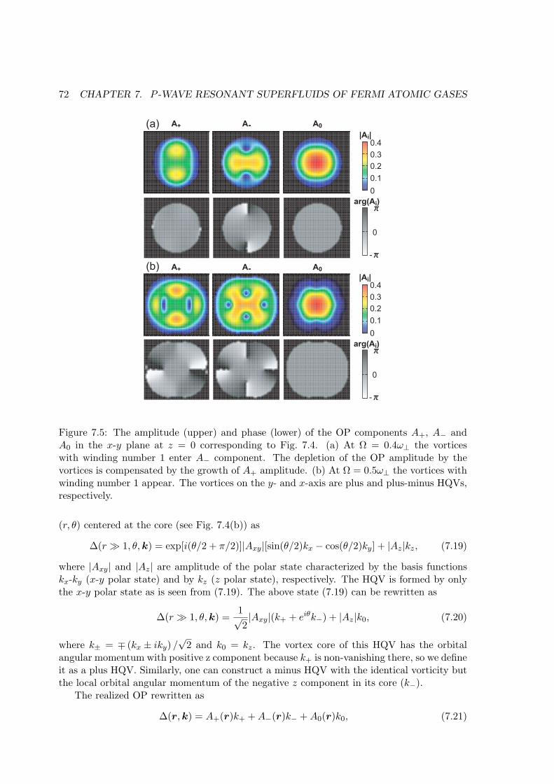
72 CHAPTER 7. P -WAVE RESONANT SUPERFLUIDS OF FERMI ATOMIC GASES
10 5
10
5(b)
(a)
0
-
arg(Ai)
0
0.1
0.2
0.3
0.4|Ai|
0
-
arg(Ai)
0
0.1
0.2
0.3
0.4|Ai|
A+ A0A-
A+ A0A-
10
10
10
10
Figure 7.5: The amplitude (upper) and phase (lower) of the OP components A+, A− andA0 in the x-y plane at z = 0 corresponding to Fig. 7.4. (a) At Ω = 0.4ω⊥ the vorticeswith winding number 1 enter A− component. The depletion of the OP amplitude by thevortices is compensated by the growth of A+ amplitude. (b) At Ω = 0.5ω⊥ the vortices withwinding number 1 appear. The vortices on the y- and x-axis are plus and plus-minus HQVs,respectively.
(r, θ) centered at the core (see Fig. 7.4(b)) as
∆(r 1, θ,k) = exp[i(θ/2 + π/2)]|Axy|[sin(θ/2)kx − cos(θ/2)ky] + |Az|kz, (7.19)
where |Axy| and |Az| are amplitude of the polar state characterized by the basis functionskx-ky (x-y polar state) and by kz (z polar state), respectively. The HQV is formed by onlythe x-y polar state as is seen from (7.19). The above state (7.19) can be rewritten as
∆(r 1, θ,k) =1√2|Axy|(k+ + eiθk−) + |Az|k0, (7.20)
where k± = ∓ (kx ± iky) /√
2 and k0 = kz. The vortex core of this HQV has the orbitalangular momentum with positive z component because k+ is non-vanishing there, so we defineit as a plus HQV. Similarly, one can construct a minus HQV with the identical vorticity butthe local orbital angular momentum of the negative z component in its core (k−).
The realized OP rewritten as
∆(r,k) = A+(r)k+ +A−(r)k− +A0(r)k0, (7.21)

7.4. PANCAKE SHAPE TRAP 73
where A± = ∓(Ax ∓ iAy)/√
2 and A0 = Az. In Fig. 7.5(a), the amplitudes (upper line) andphases (lower line) for each component A+, A−, A0 are displayed for Ω = 0.4ω⊥ correspondingto Fig. 7.4. It is seen that there are two vortices with the winding number 1 in A− componenton the y axis. The depletion of the OP amplitude by the vortices is compensated by thegrowth of A+ amplitude. The HQV is embedded in the surrounding OP field. As we walkaround one of the HQV core, the p-wave pairing state changes in the following manner: Atθ = π, the OP is described as ∆(k) = −|Axy|kx + |Az|kz, namely this is the polar state.At θ = 0, the OP is now ∆(k) = −i|Axy|ky + |Az|kz. This is a superposition of the polarstate and the chiral state. The spatial position where the arrow of l-vector near the HQVcore vanishes is the polar state, and on the opposite side of HQV core, the chiral state issuperposed by the polar state. Since this HQV breaks the reflection symmetry, the isolatedHQV is energetically disfavored and rather a pair of the HQV is advantageous. This is oneof the reasons why we found a pair of the HQV at Ω = 0.4ω⊥.
Upon further increase in the rotational speed (Ω = 0.5ω⊥), the HQVs enter further fromthe x direction (see Fig. 7.4). They are different from above mentioned plus HQVs. As isseen from Fig. 7.5(b), a pair of plus-minus HQVs appears from the x direction. There are thevortices with the winding number 1 in each A+ and A− component on the different positionof the x-axis. The depletion of the OP amplitude by the vortices is compensated by thegrowth of amplitude with the opposite orbital angular momentum component. The minusHQV is situated more inside in the trap potential than plus HQV, because of the repulsiveinteraction between the plus HQV on the x-axis and the y-axis. It is an analogous situationfor the HQVs in the F = 1 spinor BEC [129]. We also notice from Fig. 7.4 (Ω = 0.5ω⊥) thatthe condensate profile itself expands, deforms and deviates clearly from a circular form dueto the non-trivial centrifugal energy.
Figure 7.6 shows a different view of Fig. 7.4, displaying the z-x cross section. At rest, l-vectors point almost to the x direction. As Ω increases, the downward lz component appears,which causes a counterclockwise circular “orbital” supercurrent. At the top and bottom endsof the system the HQVs appear as indicated by asterisks. These blue lines show the polarstate neighboring the HQV as mentioned above. In the Ω = 0.5ω⊥ case, the side view of twopairs of plus-minus HQVs can be seen clearly. The light blue lines indicated by the red arrowscorrespond to the polar states between plus and minus HQV. These lines bend outward awayfrom the center towards ±z direction. Around the positions indicated by the red arrows thecondensate profile is greatly deformed. Because there the polar state dominates over thechiral state, which leads to the depletion of the condensate, resulting in this deformation.
7.4 Pancake shape trap
In order to understand the geometric effect of the textures stabilized in cigar shape trap, weexamine the pancake trap case. We consider the anisotropy λ = 3.0 as an example, wherewe take 100× 100× 80 meshes with the cloud size Rx = Ry = 30
√5/3 and Rz = 10
√5/3 in
the TF approximation . We fix the temperature at tx = ty = 0.5 and α = 0.95.
7.4.1 Axis symmetric texture at rest
Figure 7.7 displays the resulting l-vector texture (Fig. 7.7(a)) and associated in-plane su-percurrent (Fig. 7.7(b)) at rest. It is seen that most of the l-vectors point to the negativez direction, except for those near the upper and lower surface regions, which acquire ther-component of the radial direction. The trap potential forces the l-vector to be parallel to
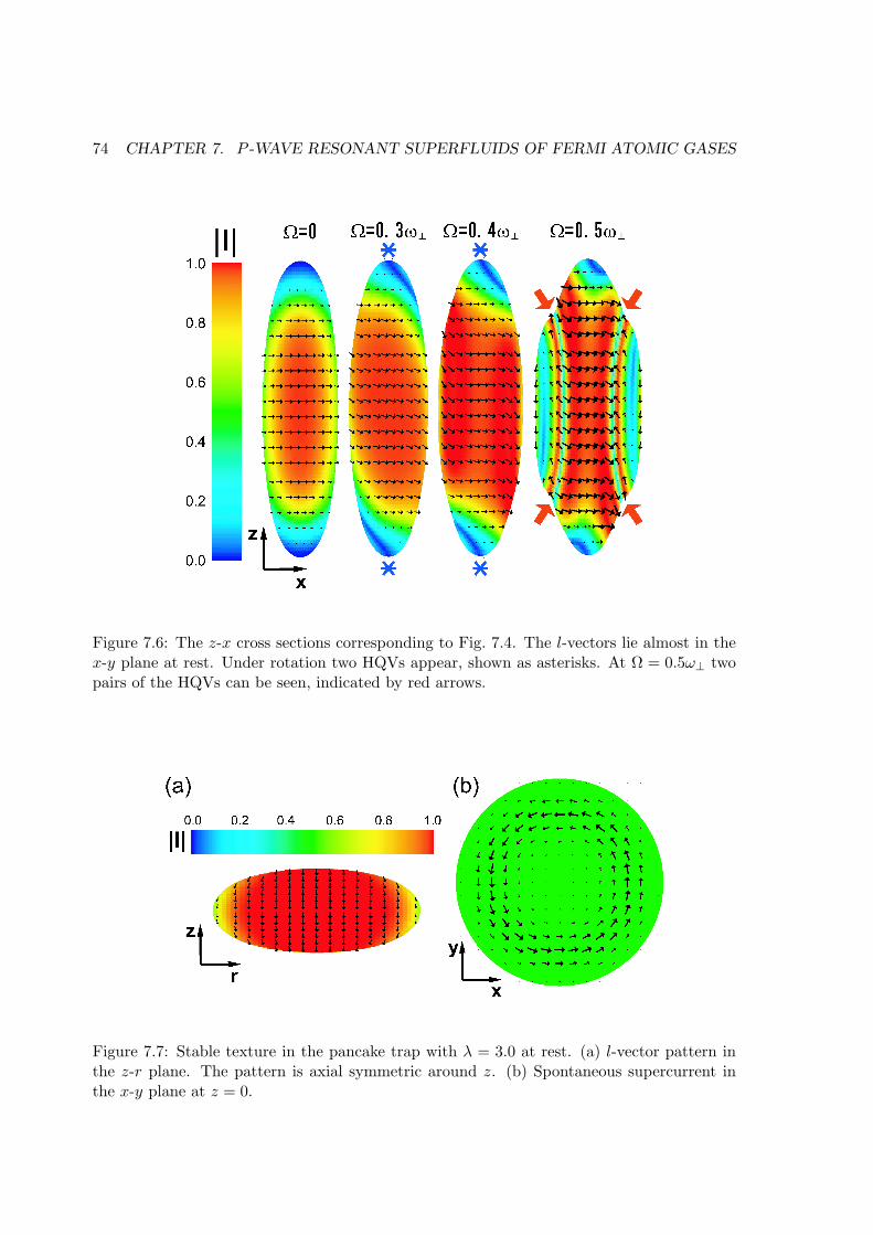
74 CHAPTER 7. P -WAVE RESONANT SUPERFLUIDS OF FERMI ATOMIC GASES
Figure 7.6: The z-x cross sections corresponding to Fig. 7.4. The l-vectors lie almost in thex-y plane at rest. Under rotation two HQVs appear, shown as asterisks. At Ω = 0.5ω⊥ twopairs of the HQVs can be seen, indicated by red arrows.
Figure 7.7: Stable texture in the pancake trap with λ = 3.0 at rest. (a) l-vector pattern inthe z-r plane. The pattern is axial symmetric around z. (b) Spontaneous supercurrent inthe x-y plane at z = 0.

7.5. QUASI-2D TRAP 75
the surface of condensates. This effect is especially strong when the curvature of the surfaceis large. Thus, in this case shown in Fig. 7.7(a), the left and right ends of the system forcethe l-vectors to point to the z direction, giving an overall l-vector configuration to the zdirection, even for the vectors near the center. The amplitude of l-vectors decrease, namelythe polar state mixes with the chiral state towards the outside.
This stable texture is axis symmetric around the z-axis, which is different in the cigarshape trap. This is because the effect of the trap potential is greater than one of the dipole-dipole interaction in the present situation (α = 0.95), so that the chiral state consisting ofthe kx and ky components dominates over the polar state, resulting in the axis symmetrictexture with respect to the z-axis. If the influence of the dipole-dipole interaction is muchgreater, or α becomes small, the stable texture is similar to those in the cigar shape trap.
The spatial variation of the amplitude of l-vectors towards the outer region generates acircular “orbital” supercurrent in the x-y plane as shown in Fig. 7.7(b). Since the spontaneoussupercurrent flows around the external rotational axis, the axial symmetric texture is stableagainst low rotation.
7.4.2 Vortices under rotation
As shown in Fig. 7.8 where the x-y cross section at z = 0 is displayed for various rotations.Similarly to the previous texture changes in the cigar shape, we see a pair of the HQV enterfrom the y-axis for Ω = 0.3ω⊥. Those vortices are exactly the same HQV as in the cigarcase (see Fig. 7.4). The following sequence upon increasing Ω is very similar to the previouscigar case, slightly differing its rotation speed where in the pancake case the sequence isshifted to lower speed. We illustrate the x-z cross section at y = 0 in Fig. 7.9. The almostl-vectors pointing to the negative z direction at rest now deforms as Ω increases. From theright and left ends the polar state seen as blue color invades into the system. At Ω = 0.5ω⊥the condensate profile itself is deformed greatly because of the dominance of the polar stateassociated with increasing HQVs.
7.5 Quasi-2D trap
A necessary condition for Majorana zero modes to exist at a vortex core is as follows: (A)the vortex possesses an odd winding number and phase singularity in spinless chiral p-wavesuperfluids [97, 130] or (B) the vortex possesses one-half winding number, that is, the vortexis a HQV in spinful chiral p-wave superfluids [41].
Here, under those circumstances, we investigate experimental requirements to satisfy thecondition (A) in spin polarized neutral atomic Fermi gases. In quasi-2D confinement thatprohibits the Cooper pairs of the z-direction, chiral kx ± iky paired states are realized unlessthe magnetic field for the Feshbach resonance is parallel to the quasi-2D system [122, 50].A requirement of the quasi-2D system is Rz ξ, namely, ~ωz/(kBTc) Tc/TF , whereRz is the radius of atomic gases toward the z-direction, ξ is the coherence length, ωz isthe trap frequency of the z-direction, Tc is the transition temperature, and TF is the Fermitemperature. This requirement may be satisfied by the optical lattice potential of a period∼ 3 µm [131, 132]. The aim of this study is to determine the stability condition for thesingular vortex, which possesses Majorana zero energy modes at the vortex core, under thequasi-2D confinement that allows the chiral kx ± iky paired state produced by the magneticFeshbach resonance. It has been proposed that the vortices with Majorana zero modes inthe p-wave resonant atomic Fermi gases are utilized for a topological quantum computer
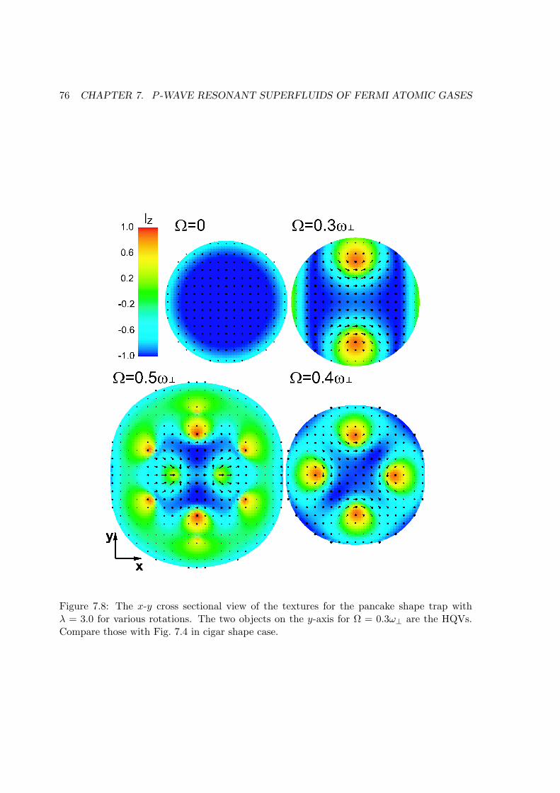
76 CHAPTER 7. P -WAVE RESONANT SUPERFLUIDS OF FERMI ATOMIC GASES
Figure 7.8: The x-y cross sectional view of the textures for the pancake shape trap withλ = 3.0 for various rotations. The two objects on the y-axis for Ω = 0.3ω⊥ are the HQVs.Compare those with Fig. 7.4 in cigar shape case.
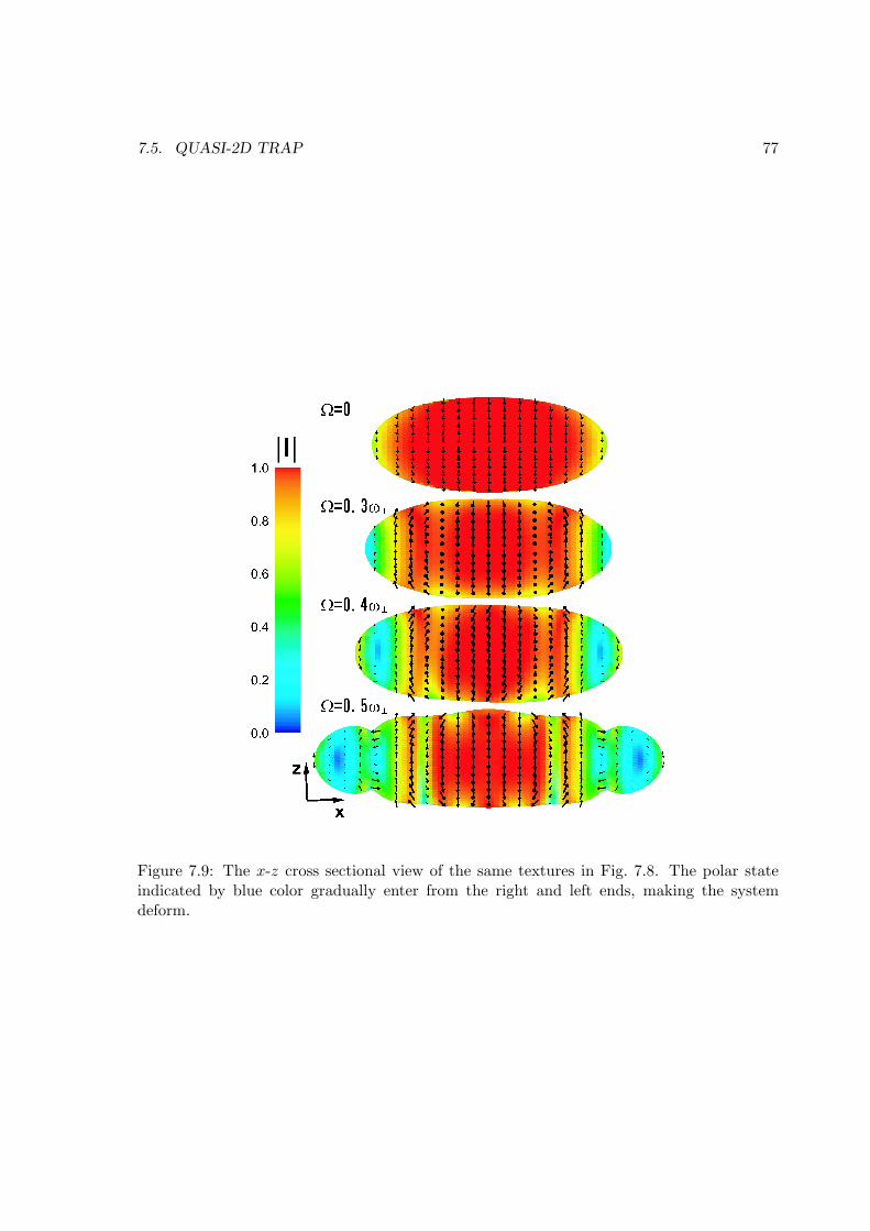
7.5. QUASI-2D TRAP 77
Figure 7.9: The x-z cross sectional view of the same textures in Fig. 7.8. The polar stateindicated by blue color gradually enter from the right and left ends, making the systemdeform.

78 CHAPTER 7. P -WAVE RESONANT SUPERFLUIDS OF FERMI ATOMIC GASES
already including the optical methods of operating and reading out states of qubits [126, 63].However, the strict stable conditions of the vortices with Majorana zero modes have not yetbeen discussed.
The OP of the spinless p-wave superfluidity in the quasi-2D trap potential can be ex-panded on the basis of rectangular coordinates with expansion coefficients Ai (i = x, y):
∆(k) = Axkx +Ayky, (7.22)
where k is the unit vector in momentum space. We assume that the momentum toward thez-direction is prohibited by the quasi-2D trap potential.
We estimate the approximate profile of the condensates at rest within the TF approxi-mation. In addition, we assume that the condensate is in the chiral state, which is stable ina bulk. The profile of OP amplitude is
|∆c(r)| =
√(1 − t) − 3
5ω2r2, (7.23)
and the radius of condensates is
R∆ =
√53
√1 − t
ω. (7.24)
Here, we introduce l-vector pointing in the direction of the orbital angular momentumof the Cooper pair. l-vector has only the z-component when the momentum toward the z-direction is suppressed. The z-component of l-vector is expressed with expansion coefficientson the basis of the component of the orbital angular momentum along the z-axis: ∆(k) =A+k+ +A−k−. By using the coefficients,
lz =|A+|2 − |A−|2
|∆|2, (7.25)
where |∆|2 = |A+|2 + |A−|2 is the squared amplitude of the OP. If the condensates are purelyin the chiral state, lz has the unit value. lz decreases when the polar state is mixed throughgradient and centrifugal energies. Finally, lz becomes zero, provided that the condensatesare in the pure polar state.
7.5.1 Possible types of axisymmetric structure and a vortex
Since we assume the axisymmetric trap potential, axisymmetric structures of the condensatesare stable when there is no vortex and only a singular vortex exists in the system. Here, wedefine the winding numbers of the plus and minus components as w+ and w−, respectively,where A± = |A±|ei(w±θ+α±) with a phase constant α±. Axisymmetric structures of the OPconsisting of the plus-minus components must have the combinations of the winding number〈w+, w−〉 = 〈n − 1, n + 1〉, where n is an integer [133, 134]. The axisymmetric conditionof what is stricter than that of multi-component spinor BECs [135]. Generally, the smallwinding number state is energetically favorable.
For the nonvortex structures, the possible combinations of the winding number are〈w+, w−〉 = 〈−2, 0〉 and 〈0, 2〉. These structures are degenerate at rest. However, under pos-itive rotation or counterclockwise rotation, the structure with 〈−2, 0〉 is stable because theminus chiral component without phase winding is advantageous under positive rotation [136].
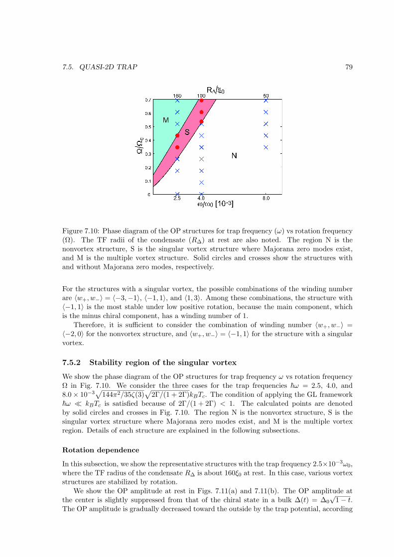
7.5. QUASI-2D TRAP 79
Figure 7.10: Phase diagram of the OP structures for trap frequency (ω) vs rotation frequency(Ω). The TF radii of the condensate (R∆) at rest are also noted. The region N is thenonvortex structure, S is the singular vortex structure where Majorana zero modes exist,and M is the multiple vortex structure. Solid circles and crosses show the structures withand without Majorana zero modes, respectively.
For the structures with a singular vortex, the possible combinations of the winding numberare 〈w+, w−〉 = 〈−3,−1〉, 〈−1, 1〉, and 〈1, 3〉. Among these combinations, the structure with〈−1, 1〉 is the most stable under low positive rotation, because the main component, whichis the minus chiral component, has a winding number of 1.
Therefore, it is sufficient to consider the combination of winding number 〈w+, w−〉 =〈−2, 0〉 for the nonvortex structure, and 〈w+, w−〉 = 〈−1, 1〉 for the structure with a singularvortex.
7.5.2 Stability region of the singular vortex
We show the phase diagram of the OP structures for trap frequency ω vs rotation frequencyΩ in Fig. 7.10. We consider the three cases for the trap frequencies ~ω = 2.5, 4.0, and8.0 × 10−3
√144π2/35ζ(3)
√2Γ/(1 + 2Γ)kBTc. The condition of applying the GL framework
~ω kBTc is satisfied because of 2Γ/(1 + 2Γ) < 1. The calculated points are denotedby solid circles and crosses in Fig. 7.10. The region N is the nonvortex structure, S is thesingular vortex structure where Majorana zero modes exist, and M is the multiple vortexregion. Details of each structure are explained in the following subsections.
Rotation dependence
In this subsection, we show the representative structures with the trap frequency 2.5×10⁻³ω0,where the TF radius of the condensate R∆ is about 160ξ0 at rest. In this case, various vortexstructures are stabilized by rotation.
We show the OP amplitude at rest in Figs. 7.11(a) and 7.11(b). The OP amplitude atthe center is slightly suppressed from that of the chiral state in a bulk ∆(t) = ∆0
√1 − t.
The OP amplitude is gradually decreased toward the outside by the trap potential, according
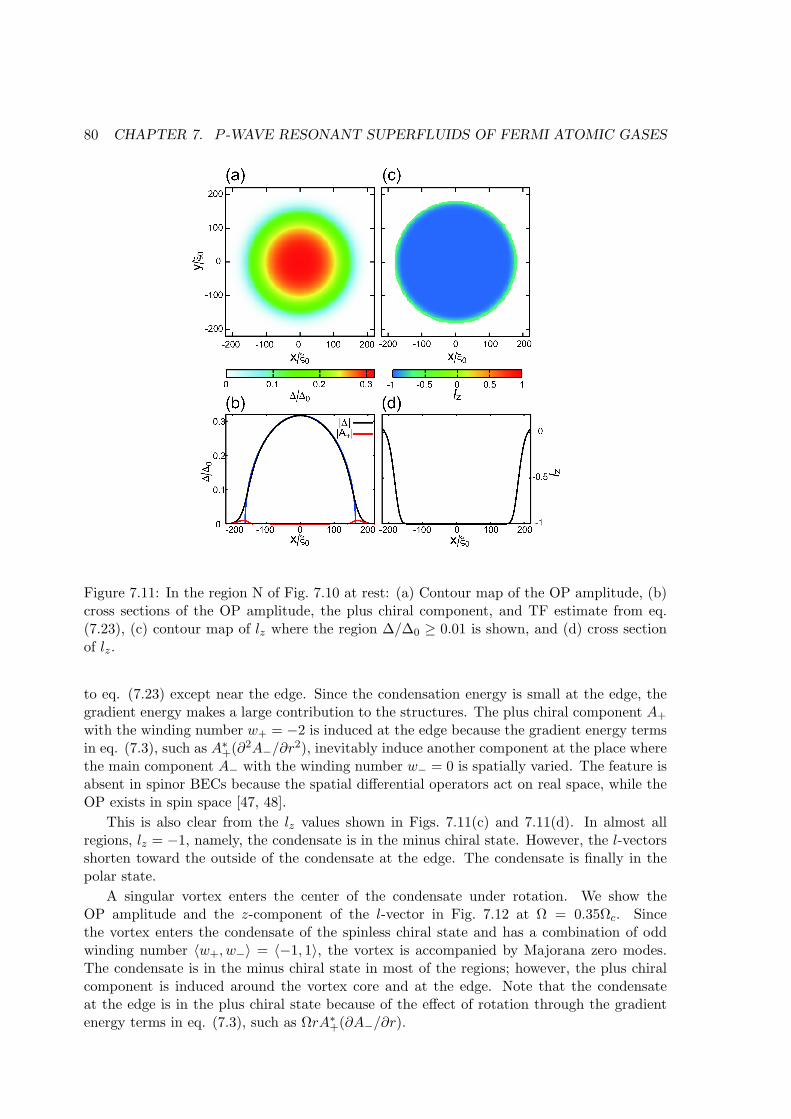
80 CHAPTER 7. P -WAVE RESONANT SUPERFLUIDS OF FERMI ATOMIC GASES
Figure 7.11: In the region N of Fig. 7.10 at rest: (a) Contour map of the OP amplitude, (b)cross sections of the OP amplitude, the plus chiral component, and TF estimate from eq.(7.23), (c) contour map of lz where the region ∆/∆0 ≥ 0.01 is shown, and (d) cross sectionof lz.
to eq. (7.23) except near the edge. Since the condensation energy is small at the edge, thegradient energy makes a large contribution to the structures. The plus chiral component A+
with the winding number w+ = −2 is induced at the edge because the gradient energy termsin eq. (7.3), such as A∗
+(∂2A−/∂r2), inevitably induce another component at the place where
the main component A− with the winding number w− = 0 is spatially varied. The feature isabsent in spinor BECs because the spatial differential operators act on real space, while theOP exists in spin space [47, 48].
This is also clear from the lz values shown in Figs. 7.11(c) and 7.11(d). In almost allregions, lz = −1, namely, the condensate is in the minus chiral state. However, the l-vectorsshorten toward the outside of the condensate at the edge. The condensate is finally in thepolar state.
A singular vortex enters the center of the condensate under rotation. We show theOP amplitude and the z-component of the l-vector in Fig. 7.12 at Ω = 0.35Ωc. Sincethe vortex enters the condensate of the spinless chiral state and has a combination of oddwinding number 〈w+, w−〉 = 〈−1, 1〉, the vortex is accompanied by Majorana zero modes.The condensate is in the minus chiral state in most of the regions; however, the plus chiralcomponent is induced around the vortex core and at the edge. Note that the condensateat the edge is in the plus chiral state because of the effect of rotation through the gradientenergy terms in eq. (7.3), such as ΩrA∗
+(∂A−/∂r).

7.5. QUASI-2D TRAP 81
Figure 7.12: In the region S of Fig. 7.10 where a singular vortex is accompanied by Majoranazero modes at Ω = 0.35Ωc: (a) Contour map of the OP amplitude, (b) cross sections of theOP amplitude (solid line) and the plus chiral component (dot-dash line), (c) contour map oflz where the region ∆/∆0 ≥ 0.01 is shown, and (d) cross section of lz.
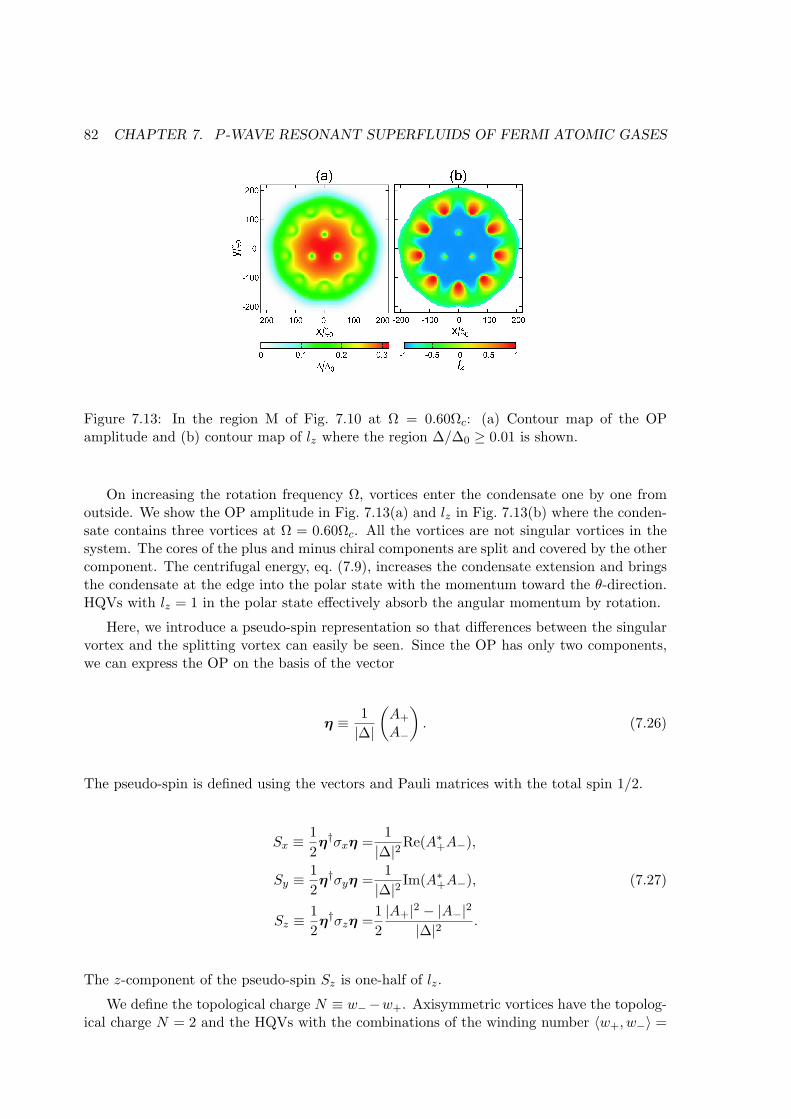
82 CHAPTER 7. P -WAVE RESONANT SUPERFLUIDS OF FERMI ATOMIC GASES
Figure 7.13: In the region M of Fig. 7.10 at Ω = 0.60Ωc: (a) Contour map of the OPamplitude and (b) contour map of lz where the region ∆/∆0 ≥ 0.01 is shown.
On increasing the rotation frequency Ω, vortices enter the condensate one by one fromoutside. We show the OP amplitude in Fig. 7.13(a) and lz in Fig. 7.13(b) where the conden-sate contains three vortices at Ω = 0.60Ωc. All the vortices are not singular vortices in thesystem. The cores of the plus and minus chiral components are split and covered by the othercomponent. The centrifugal energy, eq. (7.9), increases the condensate extension and bringsthe condensate at the edge into the polar state with the momentum toward the θ-direction.HQVs with lz = 1 in the polar state effectively absorb the angular momentum by rotation.
Here, we introduce a pseudo-spin representation so that differences between the singularvortex and the splitting vortex can easily be seen. Since the OP has only two components,we can express the OP on the basis of the vector
η ≡ 1|∆|
(A+
A−
). (7.26)
The pseudo-spin is defined using the vectors and Pauli matrices with the total spin 1/2.
Sx ≡ 12η†σxη =
1|∆|2
Re(A∗+A−),
Sy ≡ 12η†σyη =
1|∆|2
Im(A∗+A−), (7.27)
Sz ≡ 12η†σzη =
12|A+|2 − |A−|2
|∆|2.
The z-component of the pseudo-spin Sz is one-half of lz.
We define the topological charge N ≡ w−−w+. Axisymmetric vortices have the topolog-ical charge N = 2 and the HQVs with the combinations of the winding number 〈w+, w−〉 =
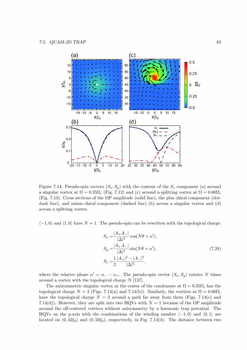
7.5. QUASI-2D TRAP 83
Figure 7.14: Pseudo-spin vectors (Sx, Sy) with the contour of the Sz component (a) arounda singular vortex at Ω = 0.35Ωc (Fig. 7.12) and (c) around a splitting vortex at Ω = 0.60Ωc
(Fig. 7.13). Cross sections of the OP amplitude (solid line), the plus chiral component (dot-dash line), and minus chiral component (dashed line) (b) across a singular vortex and (d)across a splitting vortex.
〈−1, 0〉 and 〈1, 0〉 have N = 1. The pseudo-spin can be rewritten with the topological charge:
Sx =|A+A−||∆|2
cos(Nθ + α′),
Sy =|A+A−||∆|2
sin(Nθ + α′), (7.28)
Sz =12|A+|2 − |A−|2
|∆|2,
where the relative phase α′ = α− − α+. The pseudo-spin vector (Sx, Sy) rotates N timesaround a vortex with the topological charge N [137].
The axisymmetric singular vortex at the center of the condensate at Ω = 0.35Ωc has thetopological charge N = 2 (Figs. 7.14(a) and 7.14(b)). Similarly, the vortices at Ω = 0.60Ωc
have the topological charge N = 2 around a path far away from them (Figs. 7.14(c) and7.14(d)). However, they are split into two HQVs with N = 1 because of the OP amplitudearound the off-centered vortices without axisymmetry by a harmonic trap potential. TheHQVs on the y-axis with the combinations of the winding number 〈−1, 0〉 and 〈0, 1〉 arelocated on (0, 42ξ0) and (0, 50ξ0), respectively, in Fig. 7.14(d). The distance between two

84 CHAPTER 7. P -WAVE RESONANT SUPERFLUIDS OF FERMI ATOMIC GASES
HQVs is approximately 8ξ0 ≈ 3ξ(t), where ξ(t) = ξ0(1− t)−1/2 is the temperature-dependentcoherence length.
Since the off-centered vortex has a finite OP everywhere, Majorana zero modes, whichare zero energy excitations, may not exist. Note, however, that the vortex situated at a fewtimes of coherence length is similar to the singular vortex with Majorana zero modes. Thequasi-particle states of the off-centered vortex are unknown at present. We must solve theBogoliubov-de Gennes equations in order to understand the quasi-particle states. This is ourfuture problem.
Trapping dependence
The number of vortices is proportional to the rotation frequency and the system size, or thecross section that is perpendicular to the rotational axis. The radius of the condensate isinversely proportional to the trap frequency and is increased by the centrifugal energy underrotation. Since the effect of the centrifugal energy differs among orbital states, the regionof the polar state appears predominantly at the edge of the condensate under high rotation.Therefore, the number of vortices in the chiral state situated in the central region does notincrease with increasing rotation because the angular momentum is absorbed by HQVs inthe polar state at the surrounding area, which prevent the vortex from entering the centralregion.
The vortex does not enter the chiral state up to high rotation in the case of ω = 8.0 ×10⁻³ω0 and only the singular vortex enters under high rotation in the case of ω = 4.0×10⁻³ω0.Namely, we will have to employ a low trap frequency in an experiment to observe Majoranazero modes. In the previous section under a 3D pancake-shape trap potential, the majorradius of the condensate was approximately 30ξ0, which corresponds to high-trap-frequencycases in this section; therefore, the polar core vortex with a combination of winding number〈w+, w0, w−〉 = 〈−1, 0, 1〉, which corresponds to the singular vortex 〈w+, w−〉 = 〈−1, 1〉, didnot enter the condensate.
7.6 Summary
By minimizing the generic GL energy functional within weak-coupling approximation, we findstable textures for p-wave superfluids in neutral atomic gases confined in 3D harmonic trappotentials which are to be realized in near future. In order to help detecting its superfluidity,we examine two typical trap geometries, cigar and pancake shapes. At rest, the obtainedstable textures in both shapes exhibit the spontaneous supercurrent flow. Under rotation,a pair of the HQVs enters in the condensates. The isolated HQV is never stabilized in ourcalculations because of topological constrains.
It is interesting to note that the direction of the spontaneously generated supercurrent atrest is always perpendicular to the direction of the majority l-vectors, that is, the condensatesin the cigar and pancake case l-vectors lie on the x-y plane and point to the z direction,respectively, so the supercurrent flows toward the z direction and in the x-y plane. Thisimplies that the trap shape is critical in understanding and controlling the physics of thetextures on the p-wave superfluid.
In the systems confined in the quasi-2D harmonic trap potential with a low frequency, thesingular vortex accompanied by Majorana zero modes enters the center of the condensatesunder rotation. Under high rotation, the multiple vortex state is stabilized. The off-centeredvortices in the multiple vortex state are split into two HQVs and are not accompanied by
7.6. SUMMARY 85
Majorana zero modes; the quasi-particle states of the off-centered vortex are unknown atpresent. Note that a centered singular vortex is accompanied by Majorana zero modes eventhough some vortices exist in the chiral state.
Within the present quasi-2D harmonic trap potential, there is no stable parameter regionin the (ω,Ω) plane for plural singular vortices, which is necessary for a topological quantumcomputer. We suggest the use of a quasi-2D square well potential for confinement, which isalso used in the superfluid 3He confined in parallel plates [44, 42]. This could accommodatea pair of singular vortices or more.

Chapter 8
Conclusion
8.1 Summary of this thesis
We have investigated textures and Majorana excitations such as Majorana quasi-particles(QPs) and Majorana fermions in the superfluid 3He and p-wave resonant superfluids of Fermiatomic gases.
Textures in the superfluid 3He A-phase confined in a narrow cylinder have been discussedin Chap. 5. Under magnetic fields larger than ∼ 2 mT toward the cylindrical axis, l-vectorforms radial disgyration (RD) at rest and Mermin-Ho (MH) texture under rotation. For acylinder with radius R = 50 µm, d-vector forms hyperbolic type (hb); on the other hand, fora cylinder with radius R = 115 µm, d-vector tends to form axial type (ax). Therefore, byrotation, RD-hb changes to MH-hb in the R = 50 µm cylinder and RD-ax changes to MH-hbin the R = 115 µm [19, 20]. The results correspond to results of the experiment in ISSP,Univ. of Tokyo [77, 78, 79, 80, 81].
Character of Majorana excitations is different in the superfluid 3He A- and B-phases,which have the same topological features of the spin Hall state and quantum spin Hall state,respectively. Majorana excitations in the superfluid 3He A- and B-phases confined in a thinslab have been discussed in Chap. 6. In the A-phase, Majorana QPs and Majorana fermionsexist at the side edge of the slab and dispersion relation forms “Dirac valley” [21, 22, 23].Accompanying the Majorana excitations, mass current flow along the side edge. This masscurrent has the projection of angular momentum ∼ N~/2, where N is the number of 3Heatoms. In the B-phase, Majorana fermions exist at the all surface of the slab and dispersionrelation forms Majorana cone. Accompanying the Majorana fermions, spin current flow alongthe surface three-dimensionally. If thickness of the slab is short, however, the zero energymodes of the Majorana fermions at upper and lower surfaces are split.
Textures and Majorana QPs in p-wave resonant superfluids of Fermi atomic gases havebeen discussed in Chap. 7. The p-wave resonant superfluids in three-dimensional trap poten-tial form different textures from the superfluid 3He [24, 25]. l-vector tends to align parallel tothe circumference of the condensate and spontaneous mass current flow three-dimensionallyeven at rest. Under rotation, pairs of half-quantum vortices (HQVs) enter in the conden-sate. In quasi-two-dimensional trap potential, we have derived conditions to realize a singularvortex with a Majorana QP for trap frequency and rotation frequency [26].
87
88 CHAPTER 8. CONCLUSION
8.2 Future studies
The mass current accompanying the Majorana excitations in the superfluid 3He A-phasealong the side edge of a slab has the projection of angular momentum ∼ N~/2. The valueof the projection of the angular momentum is the same as that of the intrinsic angularmomentum (IAM) by Cooper pairs of chiral p-wave superfluids. Relation between theirangular momentum is a future study. If Cooper pairs consist of all atoms in the Fermi sea,the projection of the IAM is ∼ N~/2; on the other hand, if Cooper pairs consist of atomsnear the Fermi level, the projection of the IAM is ∼ N~/2(∆/EF )2. Then, the problem ofthe IAM relates to the base of superconductivity and superfluidity. The relation may answerthe problem of the IAM had been discussed for more than three decades.
HQVs in the superfluid 3He have been investigated by NMR experiment; however, clearevidence of them has not observed yet [44]. The HQVs are stabilized by the Fermi liquidcorrection [40]; on the other hand, they are unstable under the strong-coupling effect bypressure [42, 43]. Then, the HQVs are unstable in the ordinary A-phase at high pressureand high temperature because the strong-coupling effect is greater than the Fermi liquidcorrection [138]. In thin slab with the thickness of the order of several times of the coherencelength, however, the stable region of the A-phase is enlarged toward low pressure [139]. Inthe A-phase at the low pressure, the HQVs are stabilized by the only Fermi liquid correction.A left subject is how to observe the HQVs. We may answer it to study the magnetic responseof the lattice of the HQV pairs by the quasi-classical theory.
Investigation of textures in the p-wave resonant superfluids of Fermi atomic gasses isonly our investigation by the Ginzburg-Landau theory. After realizing the p-wave resonantsuperfluids, we should do a study based on the microscopic theory to derive quantitativeresults.
Appendix A
Symmetry of quasi-classical Green’sfunction
We use the symmetry of the quasi-classical Green’s function in Eilenberger Eq. (6.1) to reducecomputational time. If we replace Matsubara frequency ωn with −ω∗
n, the quasi-classicalGreen’s functions in Nambu space have relations
g(r,k,−ω∗n) = −g(r,k, ωn)†, g(r,k,−ω∗
n) = −g(r,k, ωn)†,
f(r,k,−ω∗n) = f(r,k, ωn)†, f(r,k,−ω∗
n) = f(r,k, ωn)†, (A.1)
where we describe the complex conjugate of the Matsubara frequency explicitly because thatis important when we calculate local density of states (LDOS). By the relations, we areallowed to sum only the positive ωn to calculate self-consistent pair potential and mass andspin currents.
If we reverse the sign of relative momentum k, the sign of spin-triplet components of theorder parameter (OP) changes; on the other hand, that of a spin singlet component of theOP does not change. Specifically, general OP
∆(r,k) =(
∆↑↑(r,k) ∆↑↓(r,k)∆↓↑(r,k) ∆↓↓(r,k)
)has a relation, ∆(r,−k) = −∆T(r,k), where a superscript T indicates transposition of amatrix. Since the sign of Fermi velocity also changes, v(−k) = −v(k), the quasi-classicalGreen’s functions in particle-hole space have relations
g(r,−k, ω∗n) = g(r,k, ωn)∗, g(r,−k, ω∗
n) = g(r,k, ωn)∗,
f(r,−k, ω∗n) = −f(r,k, ωn)∗, f(r,−k, ω∗
n) = −f(r,k, ωn)∗. (A.2)
More reduction of computational time is possible by using mirror operators which defineSxa ≡ (−ax, ay, az), Sza ≡ (ax, ay,−az), and Sxza ≡ (−ax, ay,−az) with an arbitrary vectora = (ax, ay, az). If the mirror operators act on the center-of-mass coordinate of pair potentialunder the antiperiodic boundary condition mentioned in Sec. 6.2, ∆(Sr,k) = ∆(r, Sk),where S is one among Sx, Sz, and Sxz. Since Sv · S∇ = v · ∇, the quasi-classical Green’sfunction satisfies
g(Sr, Sk, ωn) = g(r,k, ωn). (A.3)
89
90 APPENDIX A. SYMMETRY OF QUASI-CLASSICAL GREEN’S FUNCTION
Therefore, the quasi-classical Green’s function and pair potential are self-consistentlyobtained by numerical calculation for only the positive Matsubara frequency and one eighthof the Fermi surface in the coordinate −L/2 ≤ x ≤ L/2 and −D/2 ≤ z ≤ D/2 by thesymmetry of the quasi-classical Green’s function (A.1), (A.2), and (A.3). The calculation forthe real space coordinates is carried out by parallel computing with OpenMP.
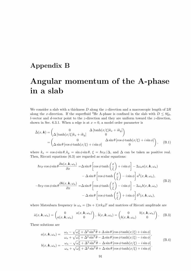
Appendix B
Angular momentum of the A-phasein a slab
We consider a slab with a thickness D along the z-direction and a macroscopic length of 2Ralong the x-direction. If the superfluid 3He A-phase is confined in the slab with D ≤ 8ξ0,l-vector and d-vector point to the z-direction and they are uniform toward the z-direction,shown in Sec. 6.3.1. When a edge is at x = 0, a model order parameter is
∆(x,k) =(
0 ∆ [tanh(x/ξ)kx + iky]∆ [tanh(x/ξ)kx + iky] 0
)=(
0 ∆ sin θ [cosφ tanh(x/ξ) + i sinφ]∆ sin θ [cosφ tanh(x/ξ) + i sinφ] 0
), (B.1)
where kx = cosφ sin θ, ky = sinφ sin θ, ξ = ~vF /∆, and ∆ can be taken as positive real.Then, Riccati equations (6.3) are regarded as scalar equations:
~vF cosφ sin θ∂a(x,k, ωn)
∂x=∆sin θ
[cosφ tanh
(x
ξ
)+ i sinφ
]− 2ωna(x,k, ωn)
− ∆sin θ[cosφ tanh
(x
ξ
)− i sinφ
]a2(x,k, ωn),
−~vF cosφ sin θ∂b(x,k, ωn)
∂x=∆sin θ
[cosφ tanh
(x
ξ
)− i sinφ
]− 2ωnb(x,k, ωn)
− ∆sin θ[cosφ tanh
(x
ξ
)+ i sinφ
]b2(x,k, ωn),
(B.2)
where Matsubara frequency is ωn = (2n+ 1)πkBT and matrices of Riccati amplitude are
a(x,k, ωn) =(
0 a(x,k, ωn)a(x,k, ωn) 0
), b(x,k, ωn) =
(0 b(x,k, ωn)
b(x,k, ωn) 0
). (B.3)
These solutions are
a(x,k, ωn) =ωn −
√ω2
n + ∆2 sin2 θ + ∆ sin θ [cosφ tanh(x/ξ) + i sinφ]
ωn +√ω2
n + ∆2 sin2 θ − ∆sin θ [cosφ tanh(x/ξ) − i sinφ],
b(x,k, ωn) = −ωn −√ω2
n + ∆2 sin2 θ − ∆ sin θ [cosφ tanh(x/ξ) − i sinφ]
ωn +√ω2
n + ∆2 sin2 θ + ∆ sin θ [cosφ tanh(x/ξ) + i sinφ].
(B.4)
91

92 APPENDIX B. ANGULAR MOMENTUM OF THE A-PHASE IN A SLAB
From eqs. (6.2), (6.4), and (6.15), quasi-classical Green’s function is
g0(x,k, ωn) =1 − a(x,k, ωn)b(x,k, ωn)1 + a(x,k, ωn)b(x,k, ωn)
=1√
ω2n + ∆2 sin2 θ
[ωn +
∆2 sin2 θ cos2 φ2(ωn + i∆sin θ sinφ)
sech2
(x
ξ
)]. (B.5)
B.1 Angular momentum by Matsubara Green’s function
From eq. (6.13), mass current is
ji(x) =mvFN0πkBT∑ωn
〈ki Im [g0(x,k, ωn)]〉k. (B.6)
Here,
Im [g0(x,k, ωn)] = − 1
2√ω2
n + ∆2 sin2 θ
∆3 sin3 θ sinφ cos2 φω2
n + ∆2 sin2 θ sin2 φsech2
(x
ξ
)= − 1
2√ω2
n + ∆2(k2x + k2
y)
∆3k2xky
ω2n + ∆2k2
y
sech2
(x
ξ
). (B.7)
For Fermi surface average, mass current has only the y-component. Since Im[g0] is evenfunction for ωn, the y-component of mass current is
jy(x) = 2mvFN0πkBT∑
ωn>0
∫ π
0
dθ sin θ2
∫ 2π
0
dφ
2πsinφ sin θ Im [g0(x,k, ωn)] . (B.8)
By the φ-integration,∫ 2π
0
dφ
2πsinφ Im [g0(x,k, ωn)]
= − ∆3 sin3 θ
2√ω2
n + ∆2 sin2 θsech2
(x
ξ
)∫ 2π
0
dφ
2πsin2 φ cos2 φ
ω2n + ∆2 sin2 θ sin2 φ
= − ∆3 sin3 θ
2√ω2
n + ∆2 sin2 θsech2
(x
ξ
)2ω2
n + ∆2 sin2 θ − 2ωn
√ω2
n + ∆2 sin2 θ
2∆4 sin4 θ
= − 14∆ sin θ
[√ω2
n + ∆2 sin2 θ +ω2
n√ω2
n + ∆2 sin2 θ− 2ωn
]sech2
(x
ξ
). (B.9)
By the θ-integration,∫ π
0
dθ sin2 θ
2
∫ 2π
0
dφ
2πsinφ Im [g0(x,k, ωn)]
= − 18∆
sech2
(x
ξ
)∫ π
0dθ sin θ
[√ω2
n + ∆2 sin2 θ +ω2
n√ω2
n + ∆2 sin2 θ− 2ωn
]
= − 18∆
sech2
(x
ξ
)[3ω2
n + ∆2
∆sin−1 ∆√
ω2n + ∆2
− 3ωn
]. (B.10)
B.2. ANGULAR MOMENTUM BY RETARDED GREEN’S FUNCTION 93
Therefore,
jy(x) = −mvFN0
4∆sech2
(x
ξ
)πkBT
∑ωn>0
[3ω2
n + ∆2
∆sin−1 ∆√
ω2n + ∆2
− 3ωn
]. (B.11)
In low temperature limit, summation of ωn = (2n+1)πkBT can be replaced by integration:
πkBT∑
ωn>0
[3ω2
n + ∆2
∆sin−1 ∆√
ω2n + ∆2
− 3ωn
]
≈πkBT
∫ ∞
0
dω
2πkBT
[3ω2 + ∆2
∆sin−1 ∆√
ω2 + ∆2− 3ω
]=
12
limω→∞
[ω
∆(ω2 + ∆2) sin−1 ∆√
ω2 + ∆2− ω2
]=
12
limω→∞
[ω
∆(ω2 + ∆2)
∆√
ω2 + ∆2+
16
∆3
(ω2 + ∆2)3/2
− ω2
]=
∆2
3. (B.12)
Finally, mass current is
jy(x) = −mvFN0∆12
sech2
(x
ξ
). (B.13)
Angular momentum of the system is derived by extending a edge circularly. Then,
Lz =2πRD∫ 0
Rdxjy(x)(R− x)
=mvFN0∆
6πRD
∫ R
0dx(R− x) sech2
(x
ξ
)=mvFN0∆
6πRDξ2 ln
(cosh
R
ξ
)≈mvFN0∆
6ξπR2D, (B.14)
because R ξ. Since ξ = ~vF /∆ and
N0 =mkF
π2~2=mkF
π2~2
1v2F
(~kF
m
)2
=3
mv2F
k3F
3π2=
3mv2
F
N
V=
3Nmv2
FπR2D
, (B.15)
angular momentum is
Lz =N~2. (B.16)
B.2 Angular momentum by retarded Green’s function
Quasi-classical retarded Green’s function is derived by analytic continuation of quasi-classicalMatsubara Green’s function as
gR0 (x,k, E) = g0(x,k, ωn)|iωn→E+iη, (B.17)

94 APPENDIX B. ANGULAR MOMENTUM OF THE A-PHASE IN A SLAB
where η is infinitesimal positive constant. From eq. (B.5), quasi-classical retarded Green’sfunction is
gR0 (x,k, E) =
1√∆2 sin2 θ − E2 − iη sgn(E)
[−iE +
∆2 sin2 θ cos2 φη + 2i(∆ sin θ sinφ− E)
sech2
(x
ξ
)]=
1√∆2(k2
x + k2y) − E2 − iη sgn(E)
[−iE +
∆2k2x
η + 2i(∆ky − E)sech2
(x
ξ
)],
(B.18)
where sgn(E) ≡ E/|E|. Mass current by retarded Green’s function is
ji(x) = mvFN0
∫ 0
−∞dE⟨ki Re
[gR0 (x,k, E)
]⟩k. (B.19)
For Fermi surface average, mass current has only the y-component. The y-component ofmass current is
jy(x) = mvFN0
∫ 0
−∞dE
∫ π
0
dθ sin θ2
∫ 2π
0
dφ
2πsinφ sin θ Re
[gR0 (x,k, E)
]. (B.20)
For the bound state −∆sin θ < E < 0,
gR0 (x,k, E) =
1√∆2 sin2 θ − E2
[−iE +
∆2 sin2 θ cos2 φη + 2i(∆ sin θ sinφ− E)
sech2
(x
ξ
)]. (B.21)
Here,
Re[gR0 (x,k, E)
]=π
∆2 sin2 θ cos2 φ√∆2 sin2 θ − E2
−12πi
[1
2(∆ sin θ sinφ− E) + iη− 1
2(∆ sin θ sinφ− E) − iη
]sech2
(x
ξ
)=π
∆2 sin2 θ cos2 φ√∆2 sin2 θ − E2
δ[2(∆ sin θ sinφ− E)] sech2
(x
ξ
). (B.22)
By the φ-integration,∫ 2π
0
dφ
2πsinφ Re
[gR0 (x,k, E)
]=
∆2 sin2 θ
2√
∆2 sin2 θ − E2sech2
(x
ξ
)∫ 2π
0dφ sinφ cos2 φ δ[2(∆ sin θ sinφ− E)]
=∆ sin θ
4√
∆2 sin2 θ − E2sech2
(x
ξ
)×[∫ 1
−1dxx
√1 − x2δ
(x− E
∆sin θ
)+∫ −1
1dxx
(−√
1 − x2)δ
(x− E
∆sin θ
)]=
E
2∆ sin θsech2
(x
ξ
). (B.23)
By the energy-integration,∫ 0
−∆sin θdE
∫ 2π
0
dφ
2πsinφ Re
[gR0 (x,k, E)
]= −∆sin θ
4sech2
(x
ξ
). (B.24)

B.2. ANGULAR MOMENTUM BY RETARDED GREEN’S FUNCTION 95
By the θ-integration,∫ π
0
dθ sin2 θ
2
∫ 0
−∆sin θdE
∫ 2π
0
dφ
2πsinφ Re
[gR0 (x,k, E)
]= −∆
6sech2
(x
ξ
). (B.25)
Therefore,
jboundy (x) = −mvFN0∆
6sech2
(x
ξ
). (B.26)
According to the same procedure below eq. (B.13), angular momentum from the bound stateis
Lboundz = N~. (B.27)
For the continuum E < −∆sin θ,
gR0 (x,k, E) = − 1√
E2 − ∆2 sin2 θ
[E +
∆2 sin2 θ cos2 φ2(∆ sin θ sinφ− E)
sech2
(x
ξ
)]. (B.28)
By the φ-integration,∫ 2π
0
dφ
2πsinφ Re
[gR0 (x,k, E)
]= − ∆2 sin2 θ
2√E2 − ∆2 sin2 θ
sech2
(x
ξ
)∫ 2π
0
dφ
2πsinφ cos2 φ
∆sin θ sinφ− E
= − ∆2 sin2 θ
2√E2 − ∆2 sin2 θ
sech2
(x
ξ
)∆2 sin2 θ − 2E(E +
√E2 − ∆2 sin2 θ)
2∆3 sin3 θ
=1
4∆ sin θ
[√E2 − ∆2 sin2 θ +
E2√E2 − ∆2 sin2 θ
+ 2E
]sech2
(x
ξ
). (B.29)
By the energy-integration,∫ −∆sin θ
−∞dE
∫ 2π
0
dφ
2πsinφ Re
[gR0 (x,k, E)
]=
14∆ sin θ
sech2
(x
ξ
)∫ −∆sin θ
−∞dE
[√E2 − ∆2 sin2 θ +
E2√E2 − ∆2 sin2 θ
+ 2E
]
=1
4∆ sin θsech2
(x
ξ
)lim
E→∞
∆2 sin2 θ + E2
√1 −
(∆sin2 θ
E
)2
−E2
=
14∆ sin θ
sech2
(x
ξ
)lim
E→∞
[∆2 sin2 θ + E2
1 − 1
2
(∆sin2 θ
E
)2
−E2
]
=∆sin θ
8sech2
(x
ξ
). (B.30)
By the θ-integration,∫ π
0
dθ sin2 θ
2
∫ −∆sin θ
−∞dE
∫ 2π
0
dφ
2πsinφ Re
[gR0 (x,k, E)
]=
∆12
sech2
(x
ξ
). (B.31)

96 APPENDIX B. ANGULAR MOMENTUM OF THE A-PHASE IN A SLAB
Therefore, from the continuum, mass current is
jconty (x) =
mvFN0∆12
sech2
(x
ξ
), (B.32)
and angular momentum is
Lcontz = −N~
2. (B.33)
Finally, total angular momentum is
Lz = Lboundz + Lcont
z =N~2. (B.34)
Appendix C
Ginzburg-Landau functional underrotation
We start with the Hamiltonian in a co-rotating frame:
H = H0 − Ω · L, (C.1)
H0 =∑
i
[(p2
i /2m)
+ U(ri)]+ V, (C.2)
where H0 is the Hamiltonian in a non-rotating system, consisting of the kinetic energy term,the harmonic trap potential term U and the interaction energy term V . The angular velocitydue to the external rotation is Ω and the angular momentum is L =
∑i 1/2 (ri × pi − pi × ri).
We can write H in the form
H =∑
i
[1
2m(pi −mvn,i)
2 + U(ri)]
+ V −∑
i
12mv2
n,i, (C.3)
where vn,i = Ω × ri is the “normal fluid” velocity at the location of the particle i. The lastterm is the centrifugal energy.
The gradient energy given by the first term of the Hamiltonian (C.3)
fgrad =7ζ(3)N(0)16(πkBTc)2
[(p∗ −mvn)iA
∗j
][(p −mvn)k Al] 〈vFikjvFkkl〉k , (C.4)
where 〈· · · 〉k denotes the Fermi surface average. Taking the contraction of the subscripts inthe Fermi surface average, the mean value is finite. Replacing p with −i~∇, we obtain thewell-known form of the gradient energy [2]
fgrad = K1(∂∗i A∗j )(∂iAj) +K2(∂∗i A
∗j )(∂jAi) +K3(∂∗i A
∗i )(∂jAj). (C.5)
In a similar manner, the centrifugal energy given by the last term of the Hamiltonian (C.3)can be recast into
fcent = − 7ζ(3)N(0)16(πkBTc)2
[(mvn)iA∗j ][(mvn )kAl] 〈vFikjvFkkl〉k (C.6)
= − m2
~2[K1(Ω × r)iA
∗j (Ω × r)iAj +K2(Ω × r)iA
∗j (Ω × r)jAi
+K3(Ω × r)iA∗i (Ω × r)jAj ]. (C.7)
97
98 APPENDIX C. GINZBURG-LANDAU FUNCTIONAL UNDER ROTATION
Taking Ω ‖ z, and Ω× r = Ωρθ, we finally obtain the expression of the centrifugal potentialas
fcent = −m2
~2Ω2ρ2(K1A
∗iAi +K2|Aθ|2 +K3|Aθ|2). (C.8)
Appendix D
Bulk energy in Ginzburg-Landaufunctional
The bulk free energy (7.7) is written as
fbulk = − (1 − tx)(|Ax|2 + |Ay|2) − (1 − αtx)|Az|2
+12(|Ax|2 + |Ay|2 + |Az|2)2 +
14(A∗2
x +A∗2y +A∗2
z )(A2x +A2
y +A2z). (D.1)
By taking Ax real, Ay = |Ay|eiθy and Az = |Az|eiθz without loss of generality, we write it as
fbulk = − (1 − tx)(|Ax|2 + |Ay|2) − (1 − αtx)|Az|2
+34(|Ax|4 + |Ay|4 + |Az|4) + (|Ax|2|Ay|2 + |Ay|2|Az|2 + |Az|2|Ax|2)
+12[|Ax|2|Ay|2 cos 2θy + |Ay|2|Az|2 cos(2θy − 2θz) + |Az|2|Ax|2 cos 2θz
]. (D.2)
There are six cases, which are possibly the minimum solutions: (i) θy = θz = 0, (ii) θy = 0,θz = π/2, (iii) θy = π/2, θz = 0, (iv) θy = π/2, θz = π/2. (v) θy = π/3, θz = 2π/3 and (vi)|Ax|2 = |Ay|2 = 0.
The relevant minimum solutions are found for (ii) and (vi). In the former case (ii) thesolution is given by
fbulk = −18[3(1 − tx)2 − 2(1 − tx)(1 − αtx) + 3(1 − αtx)2],
|Ax|2 + |Ay|2 =14[3(1 − tx) − (1 − αtx)], (D.3)
|Az|2 =14[−(1 − tx) + 3(1 − αtx)].
This solution is valid for 2 + (−3 + α)tx ≥ 0, which determines the boundary between thisphase called the A phase and the single component phase called B phase below. The othersolution for (vi) is expressed as
fbulk = −18(1 − αtx)2,
|Az|2 =23(1 − αtx).
(D.4)
This B phase is described by a single component, thus it corresponds to the so-called polarphase.
99


Bibliography
[1] D. Osheroff, R. Richardson, and D. Lee: Phys. Rev. Lett. 28 (1972) 885.
[2] D. Vollhardt and P. Wolfle: The Superfluid Phase of Helium 3 (Taylor and Francis,London, 1990).
[3] F. Wilczek: Nat. Phys. 5 (2009) 614.
[4] C. J. Pethick and H. Smith: Bose-Einstein Condensation in Dilute Gases (CambridgeUniversity Press, Cambridge, 2008).
[5] M. H. Anderson, J. R. Ensher, M. R. Matthews, C. E. Wieman, and E. A. Cornell:Science 269 (1995) 198.
[6] K. B. Davis, M. O. Mewes, M. R. Andrews, N. J. van Druten, D. S. Durfee, D. M.Kurn, and W. Ketterle: Phys. Rev. Lett. 75 (1995) 3969.
[7] C. C. Bradley, C. A. Sackett, J. J. Tollett, and R. G. Hulet: Phys. Rev. Lett. 75 (1995)1687.
[8] M. Greiner, C. A. Regal, and D. S. Jin: Nature 426 (2003) 537.
[9] S. Jochim, M. Bartenstein, A. Altmeyer, G. Hendl, S. Riedl, C. Chin, J. H. Denschlag,and R. Grimm: Science 302 (2003) 2101.
[10] M. W. Zwierlein, C. A. Stan, C. H. Schunck, S. M. F. Raupach, S. Gupta, Z. Hadzibabic,and W. Ketterle: Phys. Rev. Lett. 91 (2003) 250401.
[11] C. Regal, M. Greiner, and D. Jin: Phys. Rev. Lett. 92 (2004) 040403.
[12] M. W. Zwierlein, C. A. Stan, C. H. Schunck, S. M. F. Raupach, A. J. Kerman, and W.Ketterle: Phys. Rev. Lett. 92 (2004) 120403.
[13] J. Zhang, E. van Kempen, T. Bourdel, L. Khaykovich, J. Cubizolles, F. Chevy, M.Teichmann, L. Tarruell, S. Kokkelmans, and C. Salomon: Phys. Rev. A 70 (2004)030702.
[14] C. Schunck, M. Zwierlein, C. Stan, S. Raupach, W. Ketterle, A. Simoni, E. Tiesinga,C. Williams, and P. Julienne: Phys. Rev. A 71 (2005) 045601.
[15] Y. Inada, M. Horikoshi, S. Nakajima, M. Kuwata-Gonokami, M. Ueda, and T.Mukaiyama: Phys. Rev. Lett. 101 (2008) 100401.
[16] C. Regal, C. Ticknor, J. Bohn, and D. Jin: Phys. Rev. Lett. 90 (2003) 053201.
101
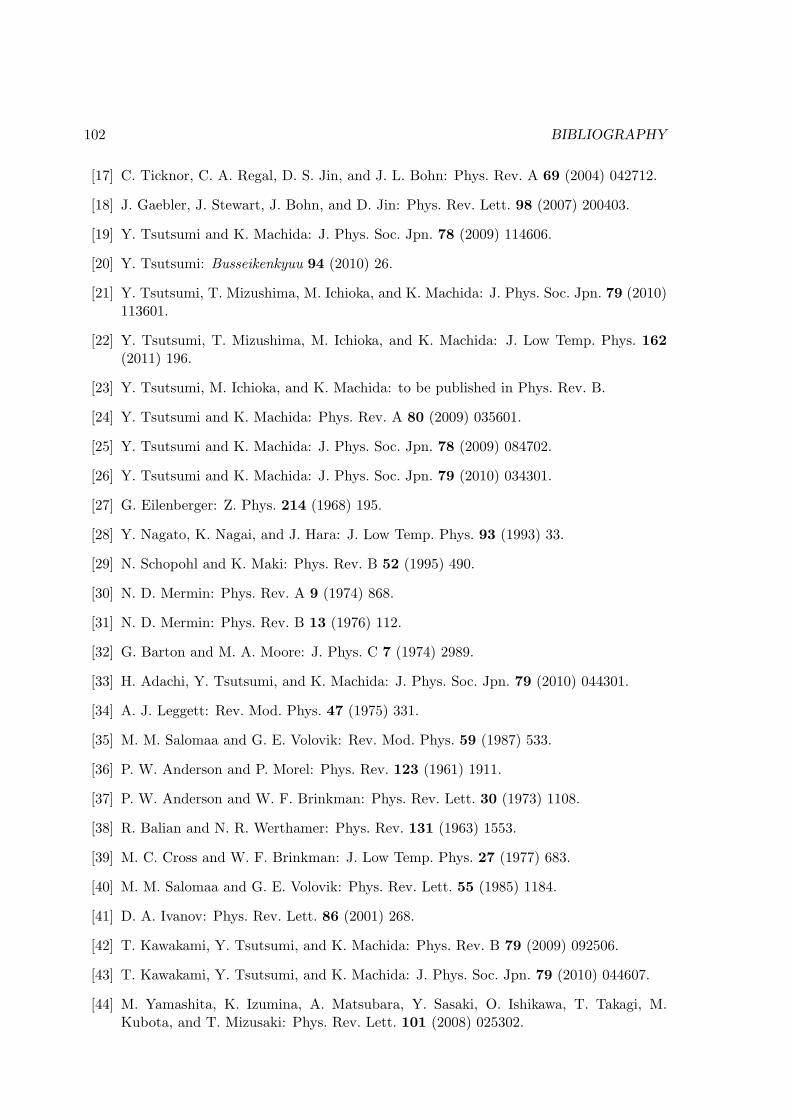
102 BIBLIOGRAPHY
[17] C. Ticknor, C. A. Regal, D. S. Jin, and J. L. Bohn: Phys. Rev. A 69 (2004) 042712.
[18] J. Gaebler, J. Stewart, J. Bohn, and D. Jin: Phys. Rev. Lett. 98 (2007) 200403.
[19] Y. Tsutsumi and K. Machida: J. Phys. Soc. Jpn. 78 (2009) 114606.
[20] Y. Tsutsumi: Busseikenkyuu 94 (2010) 26.
[21] Y. Tsutsumi, T. Mizushima, M. Ichioka, and K. Machida: J. Phys. Soc. Jpn. 79 (2010)113601.
[22] Y. Tsutsumi, T. Mizushima, M. Ichioka, and K. Machida: J. Low Temp. Phys. 162(2011) 196.
[23] Y. Tsutsumi, M. Ichioka, and K. Machida: to be published in Phys. Rev. B.
[24] Y. Tsutsumi and K. Machida: Phys. Rev. A 80 (2009) 035601.
[25] Y. Tsutsumi and K. Machida: J. Phys. Soc. Jpn. 78 (2009) 084702.
[26] Y. Tsutsumi and K. Machida: J. Phys. Soc. Jpn. 79 (2010) 034301.
[27] G. Eilenberger: Z. Phys. 214 (1968) 195.
[28] Y. Nagato, K. Nagai, and J. Hara: J. Low Temp. Phys. 93 (1993) 33.
[29] N. Schopohl and K. Maki: Phys. Rev. B 52 (1995) 490.
[30] N. D. Mermin: Phys. Rev. A 9 (1974) 868.
[31] N. D. Mermin: Phys. Rev. B 13 (1976) 112.
[32] G. Barton and M. A. Moore: J. Phys. C 7 (1974) 2989.
[33] H. Adachi, Y. Tsutsumi, and K. Machida: J. Phys. Soc. Jpn. 79 (2010) 044301.
[34] A. J. Leggett: Rev. Mod. Phys. 47 (1975) 331.
[35] M. M. Salomaa and G. E. Volovik: Rev. Mod. Phys. 59 (1987) 533.
[36] P. W. Anderson and P. Morel: Phys. Rev. 123 (1961) 1911.
[37] P. W. Anderson and W. F. Brinkman: Phys. Rev. Lett. 30 (1973) 1108.
[38] R. Balian and N. R. Werthamer: Phys. Rev. 131 (1963) 1553.
[39] M. C. Cross and W. F. Brinkman: J. Low Temp. Phys. 27 (1977) 683.
[40] M. M. Salomaa and G. E. Volovik: Phys. Rev. Lett. 55 (1985) 1184.
[41] D. A. Ivanov: Phys. Rev. Lett. 86 (2001) 268.
[42] T. Kawakami, Y. Tsutsumi, and K. Machida: Phys. Rev. B 79 (2009) 092506.
[43] T. Kawakami, Y. Tsutsumi, and K. Machida: J. Phys. Soc. Jpn. 79 (2010) 044607.
[44] M. Yamashita, K. Izumina, A. Matsubara, Y. Sasaki, O. Ishikawa, T. Takagi, M.Kubota, and T. Mizusaki: Phys. Rev. Lett. 101 (2008) 025302.
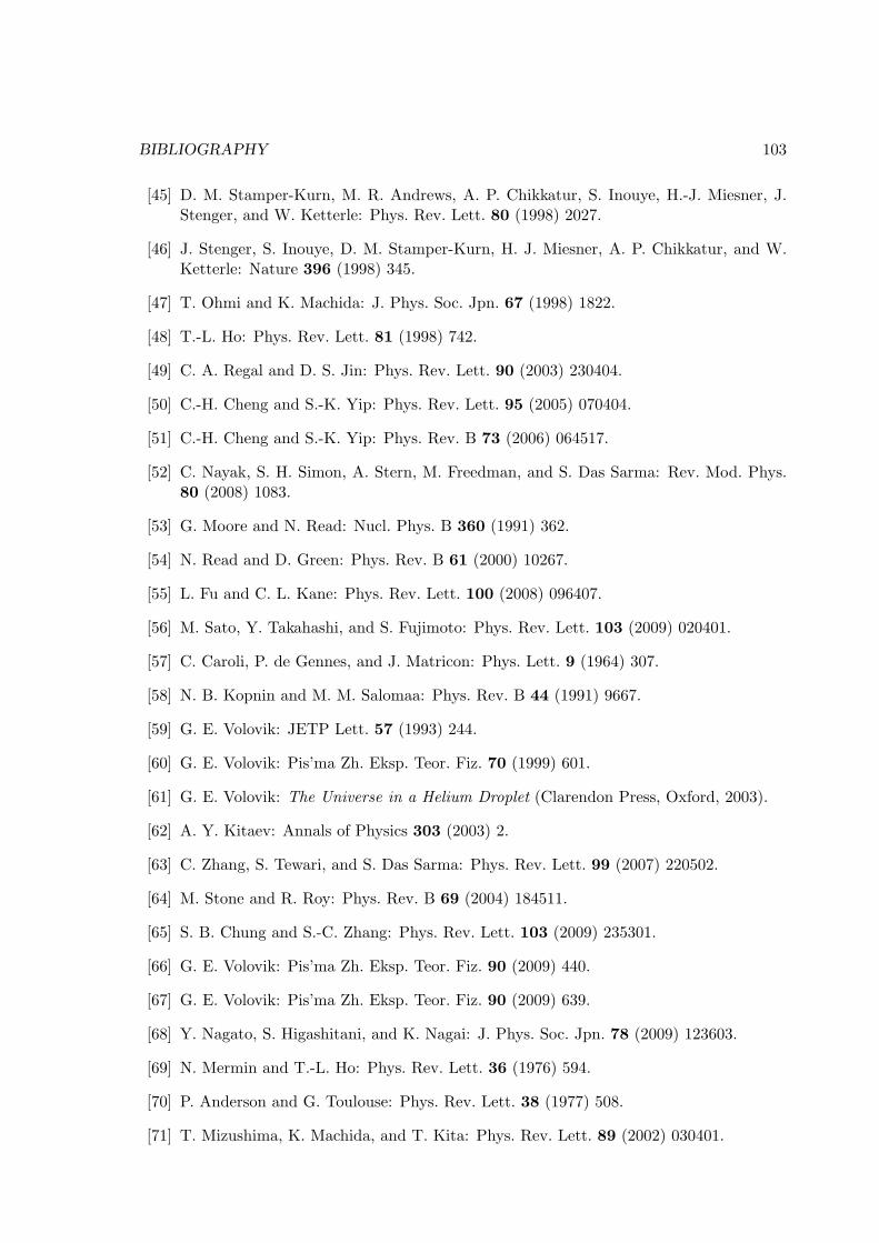
BIBLIOGRAPHY 103
[45] D. M. Stamper-Kurn, M. R. Andrews, A. P. Chikkatur, S. Inouye, H.-J. Miesner, J.Stenger, and W. Ketterle: Phys. Rev. Lett. 80 (1998) 2027.
[46] J. Stenger, S. Inouye, D. M. Stamper-Kurn, H. J. Miesner, A. P. Chikkatur, and W.Ketterle: Nature 396 (1998) 345.
[47] T. Ohmi and K. Machida: J. Phys. Soc. Jpn. 67 (1998) 1822.
[48] T.-L. Ho: Phys. Rev. Lett. 81 (1998) 742.
[49] C. A. Regal and D. S. Jin: Phys. Rev. Lett. 90 (2003) 230404.
[50] C.-H. Cheng and S.-K. Yip: Phys. Rev. Lett. 95 (2005) 070404.
[51] C.-H. Cheng and S.-K. Yip: Phys. Rev. B 73 (2006) 064517.
[52] C. Nayak, S. H. Simon, A. Stern, M. Freedman, and S. Das Sarma: Rev. Mod. Phys.80 (2008) 1083.
[53] G. Moore and N. Read: Nucl. Phys. B 360 (1991) 362.
[54] N. Read and D. Green: Phys. Rev. B 61 (2000) 10267.
[55] L. Fu and C. L. Kane: Phys. Rev. Lett. 100 (2008) 096407.
[56] M. Sato, Y. Takahashi, and S. Fujimoto: Phys. Rev. Lett. 103 (2009) 020401.
[57] C. Caroli, P. de Gennes, and J. Matricon: Phys. Lett. 9 (1964) 307.
[58] N. B. Kopnin and M. M. Salomaa: Phys. Rev. B 44 (1991) 9667.
[59] G. E. Volovik: JETP Lett. 57 (1993) 244.
[60] G. E. Volovik: Pis’ma Zh. Eksp. Teor. Fiz. 70 (1999) 601.
[61] G. E. Volovik: The Universe in a Helium Droplet (Clarendon Press, Oxford, 2003).
[62] A. Y. Kitaev: Annals of Physics 303 (2003) 2.
[63] C. Zhang, S. Tewari, and S. Das Sarma: Phys. Rev. Lett. 99 (2007) 220502.
[64] M. Stone and R. Roy: Phys. Rev. B 69 (2004) 184511.
[65] S. B. Chung and S.-C. Zhang: Phys. Rev. Lett. 103 (2009) 235301.
[66] G. E. Volovik: Pis’ma Zh. Eksp. Teor. Fiz. 90 (2009) 440.
[67] G. E. Volovik: Pis’ma Zh. Eksp. Teor. Fiz. 90 (2009) 639.
[68] Y. Nagato, S. Higashitani, and K. Nagai: J. Phys. Soc. Jpn. 78 (2009) 123603.
[69] N. Mermin and T.-L. Ho: Phys. Rev. Lett. 36 (1976) 594.
[70] P. Anderson and G. Toulouse: Phys. Rev. Lett. 38 (1977) 508.
[71] T. Mizushima, K. Machida, and T. Kita: Phys. Rev. Lett. 89 (2002) 030401.

104 BIBLIOGRAPHY
[72] A. Leanhardt, Y. Shin, D. Kielpinski, D. Pritchard, and W. Ketterle: Phys. Rev. Lett.90 (2003) 140403.
[73] W. Pogosov, R. Kawate, T. Mizushima, and K. Machida: Phys. Rev. A 72 (2005)063605.
[74] K. Wright, L. Leslie, A. Hansen, and N. Bigelow: Phys. Rev. Lett. 102 (2009) 030405.
[75] L. Buchholtz and A. Fetter: Phys. Lett. A 58 (1976) 93.
[76] L. Buchholtz and A. Fetter: Phys. Rev. B 15 (1997) 5225.
[77] R. Ishiguro: Dr. Thesis, Kyoto University (2003).
[78] R. Ishiguro, O. Ishikawa, M. Yamashita, Y. Sasaki, K. Fukuda, M. Kubota, H. Ishimoto,R. Packard, T. Takagi, T. Ohmi, and T. Mizusaki: Phys. Rev. Lett. 93 (2004) 125301.
[79] R. Ishiguro, K. Izumina, M. Kubota, O. Ishikawa, Y. Sasaki, and T. Takagi: presentedat JPS 62nd Annual Meeting (2007).
[80] K. Izumina, T. Igarashi, M. Kubota, R. Ishiguro, O. Ishikawa, Y. Sasaki, and T. Takagi:presented at JPS 2008 Autumn Meeting (2008).
[81] K. Izumina: private communication.
[82] T. Takagi: J. Phys. Chem. of Solids 66 (2005) 1355.
[83] P. de Gennes: Phys. Lett. A 44 (1973) 271.
[84] V. Ambegaokar, P. de Gennes, and D. Rainer: Phys. Rev. A 9 (1974) 2676.
[85] K. Maki: J. Low Temp. Phys. 32 (1978) 1.
[86] J. Wheatley: Rev. Mod. Phys. 47 (1975) 415.
[87] J. Sauls and J. Serene: Phys. Rev. B 24 (1981) 183.
[88] D. S. Greywall: Phys. Rev. B 33 (1986) 7520.
[89] E. Thuneberg: J. Low Temp. Phys. 122 (2001) 657.
[90] H. Choi, J. Davis, J. Pollanen, T. Haard, and W. Halperin: Phys. Rev. B 75 (2007)174503.
[91] E. Thuneberg: Phys. Rev. B 36 (1987) 3583.
[92] T. Kita: Phys. Rev. B 66 (2002) 224515.
[93] K. Aoyama and R. Ikeda: Phys. Rev. B 76 (2007) 104512.
[94] V. Ruutu, U. Parts, and K. Krusius: J. Low Temp. Phys. 103 (1996) 331.
[95] E. R. Dobbs: Helium Three (Oxford University Press, New York, 2000).
[96] T. Takagi: private communication.
BIBLIOGRAPHY 105
[97] Y. Tsutsumi, T. Kawakami, T. Mizushima, M. Ichioka, and K. Machida: Phys. Rev.Lett. 101 (2008) 135302.
[98] Y.-H. Li and T.-L. Ho: Phys. Rev. B 38 (1988) 2362.
[99] A. B. Vorontsov and J. A. Sauls: Phys. Rev. B 68 (2003) 064508.
[100] R. G. Bennett, L. V. Levitin, A. Casey, B. Cowan, J. Parpia, and J. Saunders: J. LowTemp. Phys. 158 (2010) 163.
[101] M. Saitoh and K. Kono: J. Low Temp. Phys. 148 (2007) 483.
[102] J. W. Serene and D. Rainer: Phys. Rep. 101 (1983) 221.
[103] N. Schopohl: J. Low Temp. Phys. 41 (1980) 409.
[104] M. Fogelstrom and J. Kurkijarvi: J. Low Temp. Phys. 98 (1995) 195.
[105] Y. Wada, S. Murakawa, Y. Tamura, M. Saitoh, Y. Aoki, R. Nomura, and Y. Okuda:Phys. Rev. B 78 (2008) 214516.
[106] A. B. Vorontsov and J. A. Sauls: Phys. Rev. Lett. 98 (2007) 045301.
[107] A. L. Fetter: Phys. Rev. B 14 (1976) 2801.
[108] L. J. Buchholtz and G. Zwicknagl: Phys. Rev. B 23 (1981) 5788.
[109] Y. Nagato, M. Yamamoto, and K. Nagai: J. Low Temp. Phys. 110 (1998) 1135.
[110] M. Cheng, R. M. Lutchyn, V. Galitski, and S. Das Sarma: Phys. Rev. Lett. 103 (2009)107001.
[111] T. Mizushima and K. Machida: Phys. Rev. A 82 (2010) 023624.
[112] H. Choi, J. P. Davis, J. Pollanen, and W. P. Halperin: Phys. Rev. Lett. 96 (2006)125301.
[113] Y. Okuda: private communication.
[114] R. Shindou, A. Furusaki, and N. Nagaosa: Phys. Rev. B 82 (2010) 180505.
[115] A. C. Forbes and A. F. G. Wyatt: Phys. Rev. Lett. 64 (1990) 1393.
[116] M. P. Enrico, S. N. Fisher, A. M. Guenault, G. R. Pickett, and K. Torizuka: Phys.Rev. Lett. 70 (1993) 1846.
[117] T. Okuda, H. Ikegami, H. Akimoto, and H. Ishimoto: Phys. Rev. Lett. 80 (1998) 2857.
[118] K. Kono: J. Low Temp. Phys. 158 (2010) 288.
[119] S. Murakawa, Y. Tamura, Y. Wada, M. Wasai, M. Saitoh, Y. Aoki, R. Nomura, Y.Okuda, Y. Nagato, M. Yamamoto, S. Higashitani, and K. Nagai: Phys. Rev. Lett. 103(2009) 155301.
[120] S. Murakawa, A. Yamaguchi, M. Arai, M. Wasai, Y. Aoki, H. Ishimoto, R. Nomura,and Y. Okuda: J. Low Temp. Phys. 158 (2010) 141.
106 BIBLIOGRAPHY
[121] S. Murakawa, Y. Wada, Y. Tamura, M. Wasai, M. Saitoh, Y. Aoki, R. Nomura, Y.Okuda, Y. Nagato, M. Yamamoto, S. Higashitani, and K. Nagai: J. Phys. Soc. Jpn.80 (2011) 013602.
[122] V. Gurarie, L. Radzihovsky, and A. Andreev: Phys. Rev. Lett. 94 (2005) 230403.
[123] T.-L. Ho and R. B. Diener: Phys. Rev. Lett. 94 (2005) 090402.
[124] Y. Ohashi: Phys. Rev. Lett. 94 (2005) 050403.
[125] K. Quader, R. Liao, and F. Popescu: Int. J. Mod. Phys. B 22 (2008) 4358.
[126] S. Tewari, S. Das Sarma, C. Nayak, C. Zhang, and P. Zoller: Phys. Rev. Lett. 98(2007) 010506.
[127] M. Baranov and D. Petrov: Phys. Rev. A 58 (1998) R801.
[128] M. Baranov and M. Kugan: Physica B 191 (1993) 341.
[129] A.-C. Ji, W. M. Liu, J. L. Song, and F. Zhou: Phys. Rev. Lett. 101 (2008) 010402.
[130] T. Mizushima, M. Ichioka, and K. Machida: Phys. Rev. Lett. 101 (2008) 150409.
[131] S. Stock, Z. Hadzibabic, B. Battelier, M. Cheneau, and J. Dalibard: Phys. Rev. Lett.95 (2005) 190403.
[132] Z. Hadzibabic, P. Kruger, M. Cheneau, B. Battelier, and J. Dalibard: Nature 441(2006) 1118.
[133] J. A. Sauls and M. Eschrig: New J. Phys. 11 (2009) 075008.
[134] M. Eschrig and J. Sauls: New J. Phys. 11 (2009) 075009.
[135] T. Isoshima, K. Machida, and T. Ohmi: J. Phys. Soc. Jpn. 70 (2001) 1604.
[136] M. Ichioka and K. Machida: Phys. Rev. B 65 (2002) 224517.
[137] T. Mizushima, N. Kobayashi, and K. Machida: Phys. Rev. A 70 (2004) 043613.
[138] T. Kawakami, T. Mizushima, and K. Machida: arXiv:1010.5038.
[139] K. Kawasaki, T. Yoshida, M. Tarui, H. Nakagawa, H. Yano, O. Ishikawa, and T. Hata:Phys. Rev. Lett. 93 (2004) 105301.