- 1 -

Texture Analysis Methods – A Review

Andrzej Materka and Michal StrzeleckiTechnical University of Lodz, Institute of Electronics

ul. Stefanowskiego 18, 90-924 Lodz, Polandtel. +48 (42) 636 0065, fax +48 (42) 636 2238

Email: [materka,mstrzel]@ck-sg.p.lodz.pl, Internet: http://www.eletel.p.lodz.pl

Abstract. Methods for digital-image texture analysis are reviewed based onavailable literature and research work either carried out or supervised by theauthors. The review has been prepared on request of Dr Richard Lerski,Chairman of the Management Committee of the COST B11 action“Quantitation of Magnetic Resonance Image Texture”.

1. Introduction

Although there is no strict definition of the image texture, it is easily perceived by humansand is believed to be a rich source of visual information – about the nature and three-dimensional shape of physical objects. Generally speaking, textures are complex visualpatterns composed of entities, or subpatterns, that have characteristic brightness, colour,slope, size, etc. Thus texture can be regarded as a similarity grouping in an image(Rosenfeld 1982). The local subpattern properties give rise to the perceived lightness,uniformity, density, roughness, regularity, linearity, frequency, phase, directionality,coarseness, randomness, fineness, smoothness, granulation, etc., of the texture as a whole(Levine 1985). For a large collection of examples of textures see (Brodatz 1966). Thereare four major issues in texture analysis:

1) Feature extraction: to compute a characteristic of a digital image able tonumerically describe its texture properties;

2) Texture discrimination: to partition a textured image into regions, eachcorresponding to a perceptually homogeneous texture (leads to imagesegmentation);

3) Texture classification: to determine to which of a finite number of physicallydefined classes (such as normal and abnormal tissue) a homogeneous textureregion belongs;

4) Shape from texture: to reconstruct 3D surface geometry from textureinformation.

Feature extraction is the first stage of image texture analysis. Results obtained from thisstage are used for texture discrimination, texture classification or object shapedetermination. This review is confined mainly to feature extraction and texturediscrimination techniques. Most common texture models will be shortly discussed as well.

A. Materka, M. Strzelecki, Texture Analysis Methods – A Review, TechnicalUniversity of Lodz, Institute of Electronics, COST B11 report, Brussels 1998

- 2 -

2. Texture analysis

Approaches to texture analysis are usually categorised into� structural,� statistical,� model-based and� transform

methods. Structural approaches (Haralick 1979, Levine 1985) represent texture by well-defined primitives (microtexture) and a hierarchy of spatial arrangements (macrotexture) ofthose primitives. To describe the texture, one must define the primitives and theplacement rules. The choice of a primitive (from a set of primitives) and the probability ofthe chosen primitive to be placed at a particular location can be a function of location orthe primitives near the location. The advantage of the structural approach is that itprovides a good symbolic description of the image; however, this feature is more usefulfor synthesis than analysis tasks. The abstract descriptions can be ill defined for naturaltextures because of the variability of both micro- and macrostructure and no cleardistinction between them. A powerful tool for structural texture analysis is provided bymathematical morphology (Serra 1982, Chen 1994). It may prove to be useful for boneimage analysis, e.g. for the detection of changes in bone microstructure.

In contrast to structural methods, statistical approaches do not attempt to understandexplicitly the hierarchical structure of the texture. Instead, they represent the textureindirectly by the non-deterministic properties that govern the distributions andrelationships between the grey levels of an image. Methods based on second-orderstatistics (i.e. statistics given by pairs of pixels) have been shown to achieve higherdiscrimination rates than the power spectrum (transform-based) and structural methods(Weszka 1976). Human texture discrimination in terms of texture statistical properties isinvestigated in (Julesz 1975). Accordingly, the textures in grey-level images arediscriminated spontaneously only if they differ in second order moments. Equal second-order moments, but different third-order moments require deliberate cognitive effort.This may be an indication that also for automatic processing, statistics up to the secondorder may be most important (Niemann 1981). The most popular second-order statisticalfeatures for texture analysis are derived from the so-called co-occurrence matrix (Haralick1979). They were demonstrated to feature a potential for effective texture discriminationin biomedical-images (Lerski 1993, Strzelecki 1995). The approach based onmultidimensional co-occurrence matrices was recently shown to outperform waveletpackets (a transform-based technique) when applied to texture classification (Valkealathi1998).

Model based texture analysis (Cross 1983, Pentland 1984, Chellappa 1985, Derin 1987,Manjunath 1991, Strzelecki 1997), using fractal and stochastic models, attempt tointerpret an image texture by use of, respectively, generative image model and stochasticmodel. The parameters of the model are estimated and then used for image analysis. Inpractice, the computational complexity arising in the estimation of stochastic modelparameters is the primary problem. The fractal model has been shown to be useful formodelling some natural textures. It can be used also for texture analysis and

- 3 -

discrimination (Pentland 1984, Chaudhuri 1995, Kaplan 1995, Cichy 1997); however, itlacks orientation selectivity and is not suitable for describing local image structures.

Transform methods of texture analysis, such as Fourier (Rosenfeld 1980), Gabor(Daugman 1985, Bovik 1990) and wavelet transforms (Mallat 1989, Laine 1993, Lu 1997)represent an image in a space whose co-ordinate system has an interpretation that isclosely related to the characteristics of a texture (such as frequency or size). Methodsbased on the Fourier transform perform poorly in practice, due to its lack of spatiallocalisation. Gabor filters provide means for better spatial localisation; however, theirusefulness is limited in practice because there is usually no single filter resolution at whichone can localise a spatial structure in natural textures. Compared with the Gabortransform, the wavelet transforms feature several advantages:� varying the spatial resolution allows it to represent textures at the most suitable scale,� there is a wide range of choices for the wavelet function, so one is able to choose

wavelets best suited for texture analysis in a specific application.They make the wavelet transform attractive for texture segmentation. The problem withwavelet transform is that it is not translation-invariant (Brady 1996, Li 1997).

3. Models of texture

Features (parameters) derived from AR model, Gaussian-Markov RMF model and theGibbs RMF (Derin 1987) are used for image segmentation.

3.1 AR models

The autoregressive (AR) model assumes a local interaction between image pixels in thatpixel intensity is a weighted sum of neighbouring pixel intensities. Assuming image f is azero-mean random field, an AR causal model can be defined as

∑∈

+=sNr

srrs eff θ (3.1)

where fs is image intensity at site s, se denotes an independent and identically distributed(i.i.d.) noise, Ns is a neighbourhood of s, and θθθθ is a vector of model parameters. CausalAR models have an advantage of simplicity and efficiency in parameter estimation overother, non-causal spatial interaction models. Causal AR model parameters were used in(Hu 1994) for unsupervised texture segmentation. An example of a local neighbourhoodfor such a model, represented by 4 parameters, is shown in Fig. 3.1. Shaded area in Fig. 3indicates region where valid causal half-plane AR model neighbourhood may be located.

Using the AR model for image segmentation consists in identifying the model parametersfor a given image region and then using the obtained parameter values for texturediscrimination. In the case of simple pixel neighbourhood shown in Fig. 3, that comprises4 immediate pixel neighbours, there are 5 unknown model parameters – the standard

- 4 -

deviation σ of the driving noise es and the model parameter vector θθθθ=[θ1,θ2,θ3,θ4]. Byminimising the sum of squared error

( )22 ˆ∑ ∑ −=s s

sss fe wθθθθ (3.2)

the parameters can be estimated through the following equations:

= ∑∑

−

sss

s

Tss fwww

1

θ̂θθθ (3.3)

( )222 ˆ∑ −= −

sssfN wθθθθσ (3.4)

where ws = col[fi, i∈ Ns], and the square N×N image is assumed.

sθ1

θ2 θ3 θ4

Fig. 3.1 Local neighbourhood of image element fs

Recursively identified AR model parameters were used in (Sukissian 1994) for texturesegmentation by means of an ANN classifier. Sarkar et al. (Sarkar 1997) considered theproblem of selecting the AR model order for texture segmentation.

An extensive discussion of other stochastic models, including non-causal AR model,moving average (MA) model and the autoregressive moving average (ARMA)representation can be found in (Jain 1989).

3.2 Markov random fields

A Markov random field (MRF) is a probabilistic process in which all interactions is local;the probability that a cell is in a given state is entirely determined by probabilities forstates of neighbouring cells (Blake 1987). Direct interaction occurs only betweenimmediate neighbours. However, global effects can still occur as a result of propagation.

The link between the image energy and probability is that

)/exp( TEp −∝ (3.1)

- 5 -

where T is a constant. The lower the energy of a particular image (that was generated by aparticular MRF), the more likely it is to occur.

There is a potential advantage in hidden Markov models (HMM) over other texturediscrimination methods is that an HMM attempts to discern an underlying fundamentalstructure of an image that may not be directly observable. Experiments of texturediscrimination using identified HMM parameters are described in (Povlow 1995), showingbetter performance than the autocorrelation method which required much largerneighbourhood, on both synthetic and real-world textures.

Another conventional approach segments statistical texture image by maximising the aposteriori probability based on the Markov random field (MRF) and Gaussian randomfield models (Geman 1984). Since a conditional probability density function (pdf) is notaccurately estimated by the MRF, equivalently the maximum a posteriori (MAP) estimatoruses the Gibbs random field. However, the Gibbs parameters are not known a priori,thus they should be estimated first for texture segmentation (Hassner 1981).

An efficient GMRF parameter estimation method, based on the histogramming techniqueof (Derin 1987) is elaborated in (Gurelli 1994). It does not require maximisation of a log-likelihood function; instead, it involves simple histogramming, a look-up table operationand a computation of a pseudo-inverse of a matrix with reasonable dimensions.

The least-square method for estimating the second-order MRF parameters is used in (Yin1994) for unsupervised texture segmentation by means of a Kohonen artificial neuralnetwork.

In (Yin 1994), MRF and Kohonen ANN were used for unsupervised texturesegmentation, while genetic algorithms have were applied in (Andrey 1998).

Using the MRF for colour texture segmentation was introduced in (Panjwani 1995). Amaximum pseudolikelihood scheme was elaborated for estimation model parametersfrom texture regions. The final stage of the segmentation algorithm is a merging processthat maximises the conditional likelihood of an image. The problem of selectingneighbours during the design of colour RMF is still to be investigated. Its importance isjustified by the fact that large number of parameters that can be used to defineinteractions within and between colour bands may increase the complexity of theapproach. Colour texture MRF models are considered in (Bennett 1998).

The problem of texture discrimination using Markov random fields and small samples isinvestigated in (Speis 1996). The analysis revealed that 20×20 samples contain enoughinformation to distinguish between textures and that the poor performance of MRFreported before should be attributed to the fact that Markov fields do not provideaccurate models for textured images of many real surfaces.

Multiresolution approach to using GMRF for texture segmentation appears moreeffective compared to single resolution analysis (Krishnamachari 1997). Parameters oflower resolution are estimated from the fine resolution parameters. The coarsest

- 6 -

resolution data are first segmented and the segmentation results are propagated upward tothe finer resolution.

3.3 Fractal models

There is an observation that the fractal dimension (FD) is relatively insensitive to animage scaling (Pentland 1984) and shows strong correlation with human judgement ofsurface roughness. It has been shown that some natural textures have a linear log powerspectrum, and that the processing in the human visual system (i.e. the Gabor-typerepresentation) is well suited to characterise such textures. In this sense, the fractaldimension is an approximate spectral estimator, comparable to other alternative methods(Chaudhuri 1995).

Fractal models describe objects that have high degree of irregularity. Statistical model forfractals is fractional Brownian motion (C-C. Chen 1989, Peitgen 1992, Jennane 1994). The2D fractional Brownian motion (fBm) model provides a useful tool to model texturedsurfaces whose roughness is scale-invariant. The average power spectrum of an fBmmodel follows a 1/f law; it is characterised by the self-similarity condition

Hstfstf 22 ||)]()(var[ σ=−+ (3.2)

where 0<H<1 is known as the Hurst parameter (a one-dimensional process is considered,for simplicity). The self-similarity condition is stationary in the sense that the power law isindependent of the time parameter t. The major disadvantage of fBm is that theappearance of its realisation is controlled by the single Hurst parameter H. Thus theroughness of the realisations is invariant to scale. Another disadvantage is that the modelis isotropic. The extended self similarity (ESS) model was proposed in (Kaplan 1995) todeal with these limitations, such that

)()]()(var[ 2 sgtfstf σ=−+ (3.3)

where g(1) = 1. The function g(s) is called the structure function, which determines theappearance of the 2D random model of a texture. It is related to the image correlationfunction. For the ESS model a generalised Hurst parameter is defined for isotropicimages. This parameter is scale-dependent; it is calculated by taking a logarithm of a ratioof average local energy of image horizontal and vertical increments at available scales. Theparameters derived can be used for texture analysis, as shown in (Kaplan 1995). Furtherresearch is needed to find the ESS model suitability to non-isotropic textures.

The fractal dimension D of a signal characterised by an fBm is equal to (Jennane 1994)

HED −+= 1 (3.4)

where E is the Euclidean dimension (E = 2 for a curve, E = 3 for a surface). A numberof methods for calculation of image fractal dimension is described in (S. Chen 1993,Sarkar 1994).

- 7 -

The fractal dimension of six images derived from the original texture and the concept ofmultifractal model that implies a continuous spectrum of exponents were utilised in(Chaudhuri 1995) for natural texture segmentation.

The ability of fractal features to segment mosaics of natural texture images wasinvestigated in (Duibuisson 1994). In was concluded that fractal dimensions will notsegment all types of texture.

There were attempts to segment the grey and white matters and lateral ventricles inmagnetic resonance (MR) images based on fractal models – as reported by (Lundhall1986) and (Lachman 1992).

3.4 Other models

An interesting texture model is suggested in (Doh 1996) using the metric space concept, aspecial form of the topology space. Each pixel is regarded as a set element and regionsegmentation of texture images is modelled by the topology structure of each class.Topology is a mathematically defined relationship among elements. Closure set is thelargest topology member of the set. The segmentation algorithm is based on the conceptof the metric space and closure. A number of theorems are proven in (Doh 1996) thatform the theoretical basis to the segmentation procedure. Computer simulation forsynthesised and real texture images shows that the proposed algorithm gives betterperformance than the conventional Gauss-Markov random field (GRMF) and the spatialgrey level difference method (SGLDM) methods.

4. Feature extraction techniques

4.1 First-order histogram based features

Assume the image is a function f(x,y) of two space variables x and y, x=0,1,…,N-1 andy=0,1,…,M-1. The function f(x,y) can take discrete values i = 0,1,…,G-1, where G is thetotal number of number of intensity levels in the image. The intensity-level histogram is afunction showing (for each intensity level) the number of pixels in the whole image,which have this intensity:

( )∑ ∑−

=

−

==

1

0

1

0),,()(

N

x

M

yiyxfih δ , (4.1)

where δ(j,i) is the Kronecker delta function

≠=

=ijij

ij,0,1

),(δ . (4.2)

- 8 -

The histogram of intensity levels is obviously a concise and simple summary of thestatistical information contained in the image. Calculation of the grey-level histograminvolves single pixels. Thus the histogram contains the first-order statistical informationabout the image (or its fragment). Dividing the values h(i) by the total number of pixels inthe image one obtains the approximate probability density of occurrence of the intensitylevels

NMihip /)()( = , i = 0,1,…,G-1 (4.3)

The histogram can be easily computed, given the image. The shape of the histogramprovides many clues as to the character of the image. For example, a narrowly distributedhistogram indicated the low-contrast image. A bimodal histogram often suggests that theimage contained an object with a narrow intensity range against a background of differingintensity. Different useful parameters (image features) can be worked out from thehistogram to quantitatively describe the first-order statistical properties of the image.Most often the so-called central moments (Papoulis 1965) are derived from it tocharacterise the texture (Levine 1985, Pratt 1991), as defined by Equations (4.4)-(4.7)below.

Mean: ∑−

=

=1

0)(

G

iiipµ (4.4)

Variance: ∑−

=−=

1

0

22 )()(G

iipi µσ (4.5)

Skewness: ∑−

=

− −=1

0

333 )()(

G

iipi µσµ (4.6)

Kurtosis: ∑−

=

− −−=1

0

444 3)()(

G

iipi µσµ (4.7)

Two other parameters are also used, described in (4.8) and (4.9).

Energy: ∑−

==

1

0

2)]([G

iipE (4.8)

Entropy: ∑−

=−=

1

02 )]([log)(

G

iipipH (4.9)

The mean takes the average level of intensity of the image or texture being examined,whereas the variance describes the variation of intensity around the mean. The skewnessis zero if the histogram is symmetrical about the mean, and is otherwise either positive ornegative depending whether it has been skewed above or below the mean. Thus µ3 is anindication of symmetry. The kurtosis is a measure of flatness of the histogram; the

- 9 -

component ‘3’ inserted in (4.7) normalises µ4 to zero for a Gaussian-shaped histogram.The entropy is a measure of histogram uniformity. Other possible features derived fromthe histogram are the minimum, the maximum, the range and the median value.

In the case of visual images, the mean and variance do not actually carry the informationabout the texture. They rather represent the image acquisition process, such as theaverage lighting conditions or the gain of a video amplifier. Using images normalisedagainst both the mean and variance can give better texture discrimination accuracy thanusing the actual mean and the actual variance as texture parameters (Lam 1997). Thusimages are often normalised to have the same mean, e.g. µ = 0, and the same standarddeviation, e.g. σ = 1.

Information extracted from local image histograms is used in (Lowitz 1983) as featuresfor texture segmentation. In particular, the module and state of the histogram aresuggested for quantitative texture description. For the pixel (x,y) centred in a windowcontaining N pixels, the module is

∑−

= −+−−=

1

0 )/11(/)](1)[(/)(),(

G

iMH GGNipih

GNihyxI (4.10)

It is argued in (Lowitz 1983) that the module (4.10) is a measure of information includedin the histogram. The state is the intensity level that corresponds to a maximum value ofintensity counts in the histogram.

4.2 Co-occurrence matrix based features

The major advantage of using the texture attributes (4.4)-(4.9) is obviously their simplicity.However, they can not completely characterise texture. Julesz found through his famousexperiments on human visual perception of texture (Julesz 1975), that for a large class oftextures “no texture pair can be discriminated if they agree in their second-orderstatistics”. Even if counterexamples have been found to this conjecture, the importanceof the second-order statistics is certain. Therefore the major statistical method used intexture analysis is the one based on the definition of the joint probability distributions ofpairs of pixels.

The second-order histogram is defined as the co-occurrence matrix hdθ(i,j) (Haralick1979). When divided by the total number of neighbouring pixels R(d,θ) in the image, thismatrix becomes the estimate of the joint probability, pdθ(i,j), of two pixels, a distance dapart along a given direction θ having particular (co-occuring) values i and j. Two formsof co-occurrence matrix exist – one symmetric where pairs separated by d and –d for agiven direction θ are counted, and other not symmetric where only pairs separated bydistance d are counted. Formally, given the image f(x,y) with a set of G discrete intensitylevels, the matrix hdθ(i,j) is defined such that its (i,j)th entry is equal to the number of timesthat

iyxf =),( 11 and jyxf =),( 22 (4.11)where

)sin,cos(),(),( 1122 θθ ddyxyx += (4.12)

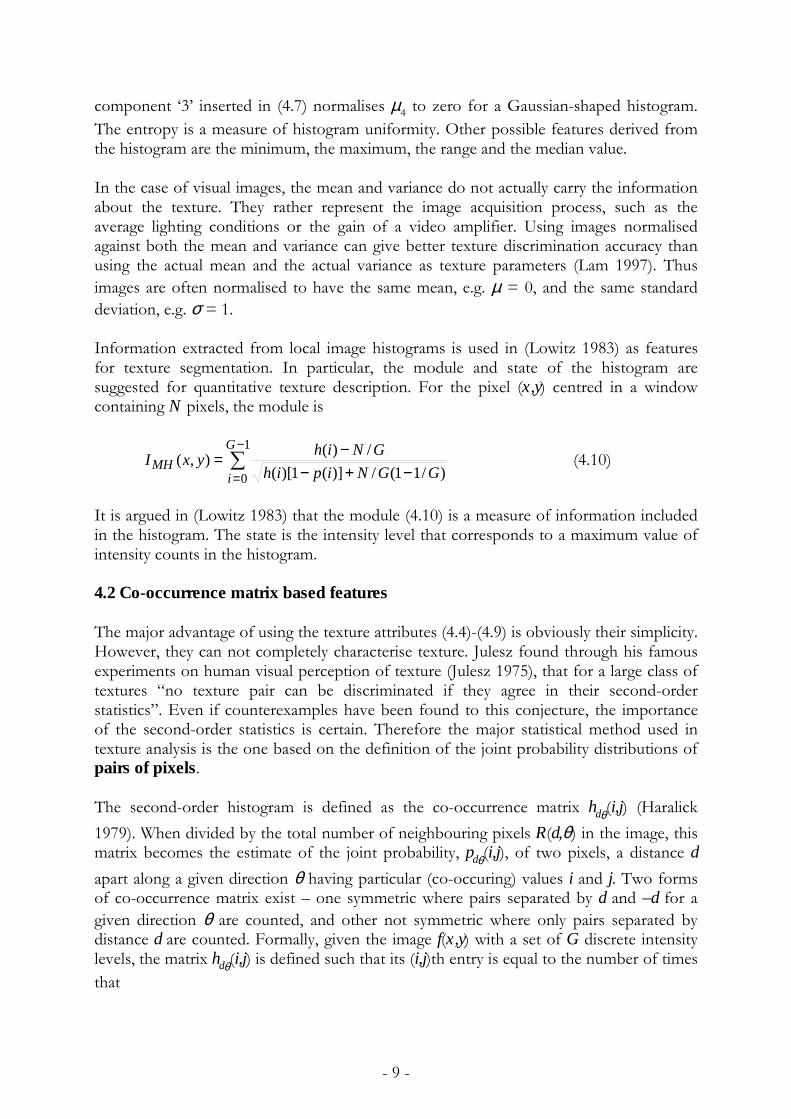
This yields a square matrix of dimension equal to the number of intensity levels in theimage, for each distance d and orientation θ. Due to the intensive nature of computationsinvolved, often only the distances d = 1 and 2 pixels with angles θ = 0°, 45°, 90° and 135°are considered as suggested in (Haralick 1979). If pixel pairs in the image are highlycorrelated, the entries in hdθ(i,j) will be clustered along the diagonal of the matrix. Co-occurrence matrix calculation is illustrated in Fig. 1, for d = 1. The classification of finetextures requires small values of d, whereas coarse textures require large values of d.Reduction of the number of intensity levels (by quantizing the image to fewer levels ofintensity) helps increase the speed of computation, with some loss of texturalinformation.

The co-occurreasonable timmatrix for thethem are defiand standard to the margina

Angular secon

Correlation:

0 0 1 10 0 1 10 2 2 22 2 3 3

- 1

Image example

h1,0°Fig. 4.1 The spatial co-occurren

rence matrix contains G2 elemee. A reduced number of featur purpose of texture discriminaned by the equations that follodeviations of the row and colul distributions px(i) and py(j)].

d moment (energy): ∑ ∑−

=

−

=

1

0

1

0[

G

i

G

j

∑ ∑−

=

−

=

−1

0

1

0

),(G

i

G

j yx

yx yjiijpσσ

µ

i\j 0 1 2 30 #(0,0) #(0,1) #(0,2) #(0,3)1 #(1,0) #(1,1) #(1,2) #(1,3)2 #(2,0) #(2,1) #(2,2) #(2,3)3 #(3,0) #(3,1) #(3,2) #(3,3)

Construction of co-occurrence matrix

4 2 1 02 4 0 01 0 6 10 0 1 2

0 -

ce ca

nts thes cation iw, wmn s

),( jip

6 0 2 00 4 2 02 2 2 20 0 2 0

h1,90°lculations (Haralick 1979)

at is too much for texture analysis in an be calculated using the co-occurrencen (Haralick 1979, Pratt 1991). Some ofhere µx, µy and σx, σy denote the meanums of the matrix, respectively [related

2] (4.13)

(4.14)

- 11 -

Inertia (contrast): ∑ ∑−

=

−

=−

1

0

1

0

2 ),()(G

i

G

jjipji (4.15)

Absolute value: ∑ ∑−

=

−

=−

1

0

1

0),(||

G

i

G

jjipji (4.16)

Inverse difference: ∑ ∑−

=

−

= −+

1

0

1

02)(1

),(G

i

G

j jijip (4.17)

Entropy: ∑ ∑−

=

−

=−

1

0

1

02 )],([log),(

G

i

G

jjipjip (4.18)

Maximum probability: ),(max,

jipji

(4.19)

An expansion of the set of features derived from the co-occurrence matrix can be foundin (Lerski 1993, Pratt 1991).

A fast algorithm for the computation of co-occurrence matrix parameters was proposedin (Alparone 1990, Argenti 1990). A generalised multidimensional co-occurrence matricesare considered in (Kovalev 1996) that exploit the co-occurrence of not only grey levels atsome distance and directions, but also such features as e.g. magnitude of local Sobelgradient. The authors called this approach “elementary structure balance method”.

An increase in the co-occurrence dimensionality, which improves the description ofspatial relationships, benefits both monochrome and colour texture segmentation(Valkealathi 1998).

4.3 Multiscale features

For calculating multiscale features, various time-frequency methods are adopted (L.Cohen 1989). The most commonly used are Wigner distributions, Gabor functions, andwavelet transforms. However, Wigner distributions are found to possess interferenceterms between different components of a signal. These interference terms lead to wrongsignal interpretation. Gabor filters are criticised for their non-orthogonality that results inredundant features at different scales or channels (Teuner 1995). Still, Gabor filters areused for texture segmentation (P. Cohen 1989, Jain 1991, Dunn 1994, Bigun 1994) andthe problem of designing Gabor filters for texture segmentation is considered in (Dunn1995, Teuner 1995). On the other hand, the wavelet transform, being a linear operation,does not produce interference terms. Unlike the Fourier transform, it possesses acapability of time (space) localisation of signal spectral features. For these reasons, muchinterest in applications of the wavelet transform to texture analysis can be noticedrecently. Dyadic wavelet transform is considered here.

- 12 -

The wavelet decomposition of a signal f(x) is performed by a convolution of the signalwith a family of basis functions, )(,2 xtsψ :

dxxxfxxf tt ss ∫∞

∞−= )()()(),( ,2,2 ψψ (4.20)

where s, t are referred to as the translation and dilation parameters, respectively.

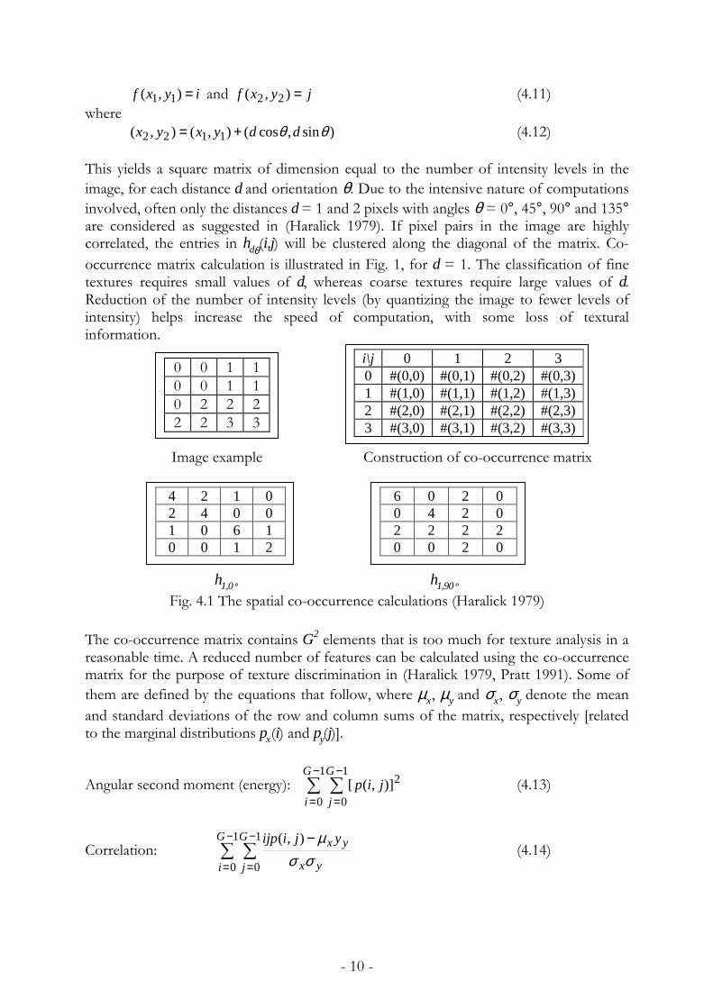
A piramidal algorithm (Mallat 1989) can perform wavelet decomposition in which a pairof wavelet filters including a lowpass filters and a highpass filter is utilised to calculatewavelet coefficients (4.20). The quadrature mirror filters (QMF) as depicted in Fig. 4.2can be used to implement wavelet transform instead of explicitly using wavelet functions(Strang 1996).

DECOMPOSITION RECONSTRUCTION

h

gf

2

2

2

2 hr

gr

Σ f

Fig. 4.2 Illustration of wavelet-based signal decomposition and reconstructiong, gr – lowpass filters; h,hr – highpass filters;

(2↓ ) – downsampling (decimation by 2); (2↑ ) – upsampling.

h

g

f 2

22

2

h

g

LH

LL

H

L

Fig. 4.3 Signal analysis using 2 levels of dyadic wavelet decompositionL – approximation components, H – detail components

In the case of two-dimensional images, the wavelet decomposition is obtained withseparable filtering along the rows and along the columns of an image (Mallat 1989). Fig.4.4 illustrates the level 1 (1-scale) and level 2 (2-scale) image decomposition.

The wavelet analysis can thus be interpreted as image decomposition in a set ofindependent, spatially oriented frequency channels. The HH subimage represents diagonaldetails (high frequencies in both directions – the corners), HL gives horizontal highfrequencies (vertical edges), LH gives vertical high frequencies (horizontal edges), and theimage LL corresponds to the lowest frequencies. At the subsequent scale of analysis, theimage LL undergoes the decomposition using the same g and h filters, having always the

- 13 -

lowest frequency component located in the upper left corner of the image. Each stage ofthe analysis produces next 4 subimages whose size is reduced twice compared to theprevious scale. Good texture segmentation results can be obtained within 2 to 4 scales ofwavelet decomposition. In the case of a 3-scale analysis, 10 frequency channels can beidentified as shown in Fig. 4.5. The size of the wavelet representation is the same as thesize of the original image. As there is a choice of particular wavelet function for imageanalysis, symmetric wavelet functions appear superior to non-symmetric ones (Lu 1997)which is attributed to the linear-phase property of symmetric filters.

LH

HL HH

LL

LLLH

LLHL LLHHLH

HL HH

LLLL

Fig. 4.4 One-scale decomposition (left), two-scale decomposition (right)

1 2

3 45

6 7

8

9 10

HHLH

LL HL

Fig. 4.5 Ten channels of a threee-level wavelet decomposition of an image

In (Porter 1996) wavelet transform is used both to analyse the image prior tosegmentation enabling feature selection as well as to provide spatial frequency-baseddescriptors for segmenting textures. The quality and accuracy of segmentation ultimatelydepend on the type of features used. Images consisting of a number of textured regionsare best segmented using frequency-based features, whereas images made up of smootherregions can more easily be segmented using local mean and variance of intensity levels.

- 14 -

Different features are required in different regions of the image. Three-level waveletdecomposition was used in (Porter 1996), resulting in 10 main wavelet channels. The“energy” of each channel can be evaluated by simply calculating the mean magnitude ofits wavelet coefficients.

∑ ∑−

=

−

==

1

0

1

0|),(|1 M

x

N

yn yxw

MNC (4.21)

where the channel is of dimensions M by N (usually M = N) and w is a wavelet coefficientwithin a channel. It turns out that textured images have large energies in both low andmiddle frequencies. The low-frequency channels are dominant over smooth regions.

Fig. 4.6 Example energy levels for smooth and textured images

To decide what kind of features to use for image segmentation, the image is first split intosmooth and textured regions based on the value of the following factor

765

4321CCC

CCCCR++

+++= (4.22)

The region is labelled as smooth if R ≥ T or textured if R < T, where T is the threshold.Appropriate features are then selected for the regions, to perform the segmentation asillustrated in Fig. 4.7.

WaveletAnalysis

FeatureSelection

ClusteringOriginalImage

SegmentedImage

Fig. 4.7 Block diagram of the segmentation algorithm (Porter 1996)

4.4 Other features

A Grey-Tone Difference Matrix (GTDM) was suggested in (Amadasun 1989) in anattempt to define texture measures correlated with human perception of textures. A GTDmatrix is a column vector containing G elements. Its entries are computed based on

0

20

40

60

80

1 2 3 4 5 6 7 8 9 10

Channel number

Ener

gy SmoothTextured

- 15 -

measuring the difference between the intensity level of a pixel and the average intensitycomputed over a square, sliding window centred at the pixel. Suppose the image intensitylevel f(x,y) at location (x,y) is i, i=0,1,…,G-1. The average intensity over a window centredat (x,y) is

∑ ∑−= −=

++−

==K

Km

K

Kni nymxf

Wyxff ),(

11),( (4.20)

where K specifies the window size and W = (2K+1)2. The i-th entry of the gray-tonedifference matrix is

∑ ∑−

=

−

=−=

1

0

1

0||)(

M

x

N

yifiis (4.21)

for all pixels having the intensity level i. Otherwise, s(i) = 0.

Five different features were derived from the GTDM, to quantitatively describe suchperceptual texture properties as� coarseness (defined by the size of texture primitives):

11

0cos )(

−−

=

+= ∑

G

ii ispC ε (4.22)

where ε is a small number to prevent the coarseness coefficient becoming infinite andpi is the estimated probability of the occurrence of the intensity level i

nNp ii /= (4.23)with Ni denoting the number of pixels that have the level i, and n = (N-K)(M-K).

� contrast (dependent on the intensity difference between neighbouring pixels):

−

−= ∑∑ ∑

=

−

=

−

=

G

i

G

i

G

jji

ttcon is

njipp

NNC

0

1

0

1

0

2 )(1)()1(

1 (4.24)

� busyness (described by high spatial frequency of intensity changes):

∑ ∑

∑

−

=

−

=

−

=

−= 1

0

1

0

1

0

||

)(

G

i

G

jji

G

ii

busjpip

ispC , 0,0 ≠≠ ji pp (4.25)

� complexity (dependent on the number of different primitives and different averageintensities):

[ ]∑ ∑−

=

−

=+

+−=

1

0

1

0)()(

)(||G

i

G

jji

jicom jspisp

ppnjiC , 0,0 ≠≠ ji pp (4.26)

� texture strength (clearly definable and visible primitives):

- 16 -

∑

∑ ∑

−

=

−

=

−

=

+

−+

= 1

0

1

0

1

0

2

)(

))((

G

i

G

i

G

jji

stris

jipp

Cε

, 0,0 ≠≠ ji pp (4.27)

The original paper (Amadasun 1989) contains more detailed explanation about thereasoning that led to the particular definition of texture features given by Equations(4.22)-(4.27).

Examples of commonly used features, not discussed above, are� Fourier transform energy,� local extrema count along a 1D scan direction (Mitchell 1977),� run length matrix-derived features (Haralick 1979),� directional intensity level energy (Hsiao 1989),� filter masks in the space domain (multichannel filtering, Law features) including

Gabor filters (P. Cohen 1989, Jain 1991, Dunn 1994, Bigun 1994) and subsequentnonlinear operators (Cohen 1990, Jain 1996),

� filter masks in the Fourier spectrum domain (Delibasis 1997),� mathematical morphology-derived features (Chen 1994, Lam 1997),� statistical geometrical features (Y. Chen 1995: 16 features that describe geometry of

binary images obtained from texture by multithresholding).

4.5 Feature selection

� (Fukunaga 1990): Choosing most effective features for class separability (different tothe criteria for image representation).

� (Lerski 1993): Strongly skewed features are rejected; strongly correlated features arerejected. Discriminatory analysis is used to select the most discriminating features (ananalysis of variance F-test was applied).

� (Kovalev 1996): The most desirable line of approach is to pay a lot of attention inchoosing image features so that the classes are linearly separable. In other words,careful feature selection followed by a simple classifier is much more preferable than aquick feature selection stage followed by a carefully designed classifier.

5. Texture discrimination and segmentation

The reported segmentation methods are based on:� region growing (Pratt 1991, Gonzalez 1992),� estimation theory – maximum likelihood (Chellappa 1985),� split-and-merge (Chen 1979, Pratt 1991, Gonzalez 1992),� Bayesian classification (Hsiao 1989),� probabilistic relaxation – iterative approach for using context information to reduce

local ambiguities (Hsiao 1989),� clustering (Hu 1994),� artificial neural networks (Jain 1991, Sukissian 1994, Yin 1994, Augusteijn 1995,

Strzelecki 1995, Jain 1996, Bruzzone 1998).

- 17 -

The techniques for texture segmentation can be classified to be either supervised (Hsiao1989a, Unser 1990, Reed 1990, Bovik 1990, Dunn 1994, Dunn 1995) or unsupervised(Hsiao 1989b, Jain 1991, Mao 1992, Bigun 1994, Hu 1994, Yin 1994, Chaudhuri 1995, J.Chen 1995, Panjwani 1995, Kervrann 1995, Teuner 1995, Andrey 1998) based on whetherthe number of textures contained in the image is known in advance or not.

The most recent contributions are shortly characterised below, as they may put some lighton current trends in the field.

The k-means clustering technique was used in (Porter 1996), applied to wavelet derivedfeatures. The technique involves grouping those pixels in the image whose feature vectorsrepresent points that are close together in the feature space. The final result is a numberof clusters K, where each hopefully depicts a perceptually different region in the image.

Feedforward ANNs were used in (Jain 1996) along with multichannel filtering for texturesegmentation. A backpropagation algorithm was applied for the classifier training.

Improvements to iterative morphological decomposition were proposed in (Lam 1997)for rotation-invariant texture discrimination, based on features derived usingmathematical morphology. The method is compared to simultaneous autoregressive(SAR) models and multichannel Gabor filters.

A comparison is presented in (Porter 1997) between the performance of three schemes offeature extraction: the wavelet transform, a circularly symmetric Gabor filter and a GMRFwith a circular neighbour set to achieve rotation-invariant texture discrimination. Inconclusion, the wavelet-based approach was the most accurate, exhibited the best noiseperformance and had the lowest computational complexity when implemented using thedb4 wavelet.

Experiments with natural textures were performed in (Valkealathi 1998) using reducedmultidimensional co-occurrence histograms. They proposed linear compression,dimension optimisation and vector quantization for the reduction of histograms. As aresult, higher classification accuracy was obtained compared to the channel histogramsand wavelet packets.

The problem always encountered in textured image segmentation relates to the trade-offbetween the sample size and accuracy. The bigger the sample size, the better the accuracyof feature estimation; however, this allows a coarse segmentation only. Imagesegmentation at small sample size is tackled in (Speis 1996) where RMF was used as imagemodel. Boundary effect (a pixel at texture boundary has neighbouring pixels belonging todifferent textures) is investigated in (Yhann 1995) where multiresolution method wascombined with detecting local intensity discontinuities at the boundary.

- 18 -

6. MRI Texture Classification

A limited number of recently published contributions is quoted here, as a result of theearly stage of this literature survey. [(?) denotes a situation in which original papers were notaccessible to the authors at the time of completing the manuscript of this survey.]

� (Lundhall 1986): Segmentation of grey and white matter and lateral ventricles using afractal model (?).

� (Lachmann 1992): Fractal model (?).� (Bello 1994): Combination of wavelet analysis and multiresolution MRF. First, discrete

wave-packet transform is used to focus on selected image “channel” data. Second, anMRF segmentation is used to “fuse” data associated with the selected image channelsat a specific resolution levels. Applied to brain image segmentation to distinguish“empty space”, “white matter”, “grey matter”, “internal brain cavities” and“neck/muscle/skin”. Qualitative characteristics of the derived segmentation describedas “good”.

� (Delibasis 1997): Genetic algorithm-designed filter masks correlated with imageFourier spectrum. Segmentation of cerebellum from MR images.

� (Bruzzone 1998): Magnetic resonance images supervised classification using so-calledstructural neural networks shows more accuracy than a k-NN classifier. Images werefirst segmented using a region-growing algorithm. Each region was represented by afeature vector (features related to intensity, position and size-and-shape) to excite theSNN. Twelve classes were associated with different organs (e.g. the nose, the left eye,the brain, etc.).

7. Work carried out at the Institute of Electronics, TUL

A number of different methods concerning texture analysis and synthesis has beendeveloped in the Institute of Electronics since 1990. For purposes of texture analysis andsegmentation statistical methods using co-occurrence matrix, micro-feature extraction andMarkov random field models were implemented. Among these methods, the multilayerperceptron (MLP) network and the cellular neural network (CNN) were utilised. Texturesynthesis methods were based on the CNN approach.

7.1 Co-occurrence matrix method

This statistical approach, which is based on co-occurrence matrices (Haralick 1979)describes second-order statistics of texture. An algorithm for co-occurrence matrixconstruction and statistical feature extraction from the matrix may be defined as follows:a) Division of analysed image into connected and disjoint regions. An image is

considered as a set of points distributed on two-dimensional and finite space.Intensities of image points are integer values from range [0,...,G-1] where G is thenumber of intensity levels.

b) Construction of co-occurrence matrix H for each region and some vectors v, whereH[i,j] is a matrix of estimated probabilities of transitions from level i to level j for

- 19 -

given vector v where i,j = 0,1,...,G-1, and vector v defines direction of construction ofH and distance between points that have intensities i and j.

c) Computation of R statistical features considered as representative for a given class oftexture, derived from matrix H.

d) Classification of textures using a classifier with R inputs and K outputs, where K isnumber of classes.

As a classifier, the multilayer perceptron (MLP) artificial neural network was used fortextured image segmentation in (Strzelecki 1995). The single-hidden layer architecture ofthe MLP is illustrated in Fig. 7.1. The texture features are fed to the network inputs. Thelayer of hidden processing elements links the network input and output. The number ofoutput neurons is set according to the number of texture classes. The index of an outputneuron that shows a maximum activation level indicates the texture class that correspondsto actual ANN input. Thanks to the non-linear activation function fs of the networkelements, the MLP can form arbitrary complex decision boundaries in the classifiedfeature space.

MLP is trained with the supervised learning algorithm known as the backpropagation ofthe gradient of the error, i.e. the difference (defined usually by the minimum mean squarevalue criterion) between the actual and desired network output (Hecht-Nielsen 1990).Computational cost of the training stage heavily depends on the number of neurons inthe network. Also, more importantly, the number of neurons determines networkclassification capabilities.

Fig. 7.1 MLP artificial neural network (fs denotes the nonlinear activation function)

The choice of the number and the type of statistical features computed using the co-occurrence matrixes was made based on multidimensional variance analysis, whichprovides optimal set of features for given segmentation task.

NETWORK INPUTS

HIDDEN LAYER

WR L

WL K

OUTPUT LAYER

- 20 -

Examples of texture segmentation using the co-occurrence matrix method are presentedin Fig. 7.2a and 7.2b. They represent cross-section of human skin tissue: epidermis –region marked with ‘1’, dermis (‘2’) and the mast cells (‘3’). The problem was to find thearea occupied by the mast cells that is important in diagnosis of some kinds of skincancers (for example urticaria pigmentosa). Both pictures are represented as arrays of512×512 pixels with 128 intensity levels.

(a) (b)

Fig. 7.2 Skin tissues after segmentation

The image shown in Fig. 7.3 presents mast cells and their position with respect todermoepidermal junction. The CM method was used to find this junction. The measureddistance of mast cells to this junction is one of important characteristics of mast cellsmorphology.

The aim of this study was to elaborate a texture analysis method that would allowdescribing morphology and localisation of mast cells in the skin. This research wasperformed with collaboration of Department of Dermatology, Medical University ofLodz.

Fig. 7.3 Mast cells (white) and the dermoepidermal junction (staircase line)

- 21 -

7.2 Texture segmentation based on micro-feature extraction

In this approach the texture is assumed to contain random/periodic transitions of imagebrightness, called micro-features (Pelczynski 1994), e.g. edges, line segments or set of pointswhich have specific spatial intensity distribution. These local features can be extracted byperforming two-dimensional convolution of an image with a particular filter mask thatrepresents a model of the micro-feature pattern. Then, if required, a further nonlineartransformation of the image obtained after the convolution may be performed. Examplesof 3 3× masks used for local feature detection are illustrated in Fig. 7.4.

-1 -1

-1 -1

0

0

0

0 4

-1

-1

-1

-1

-1

-1

1

1

-2 2

0

0

0 -2 -2

2

4

2

a) b) c)Fig. 7.4 Examples of micro-feature detection masks: a) point detector, b) vertical edge

detector, c) vertical line-like structure detector

As in the co-occurrence matrix method, the calculated feature values are fed to MLPnetwork, which is used as a classifier. An example of segmentation of sample biomedicalimage is presented in Fig. 7.5.

1

2

3

1

a) b)

Fig. 7.5 Segmentation of sample microscopic image representing biological tissues:a) source image with three texture classes, b) image after segmentation.

In the next approach, a cellular neural network (CNN) was used both for texture featureextraction and texture segmentation. CNNs is an array of nonlinear filters with localfeedback connections that enhance their filtering capabilities. A single CNN table is atwo-dimensional array composed of identical computational elements, or cells (Figs. 7.6and 7.7). Each element has input and is locally connected with other cells in the network.Weights between all inputs and the element, from its neighbourhood, form the so-calledweight template. The weight template is identical for every element in a network. Fig. 7.8illustrates the proposed network structure for texture classification.

- 22 -

Fig. 7.6 An array of cellular neural network cells of neighbourhood 1

Fig. 7.7 Block diagram of a single CNN cell

Fig. 7.8 Cellular neural network architecture for texture segmentation

First layer of the network consists of CNN tables, each associated with one class ofrecognisable texture. Each of these CNN tables detects local features of only one textureand remains insensitive to others. Second network layer performs linear averaging of thefirst layer outputs, providing statistical measure of detected local texture features.Intensities of considered feature maps serve as inputs to the classification layer. In theexperiments, a very simple classification rule was implemented which assumed that thehighest output of feature map indicates proper texture class. Two-dimensional array of

Third layer

Second layer

First layer

A-r,-r

Ar,r

B-r,-r

Br,r

Σ ∫

•

•

•

•

↑↑↑↑

yk,l

I

uk,l

yi,j

ui,j

xi,j

- 23 -

such classifiers can form the third network layer. This structure performs fully paralleltexture segmentation process. In case of hardware network realisation it provides real-time image segmentation. For template elements setting, genetic algorithm was used(Pelczynski 1997).

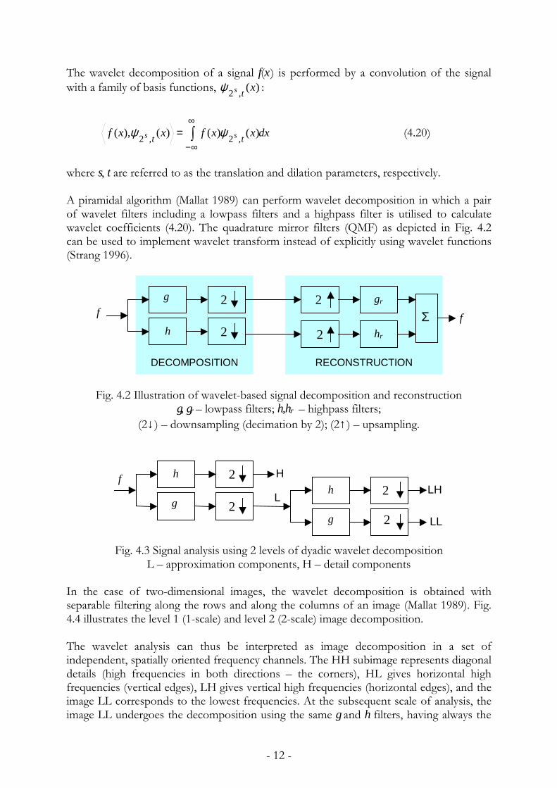
The proposed CNN model for texture segmentation was tested on images derived fromthe Brodatz album. An example of segmentation results is shown in Fig. 7.9.

(a) (b)Fig. 7.9 Example of texture classification using CNN

a) original image, b) image after segmentation

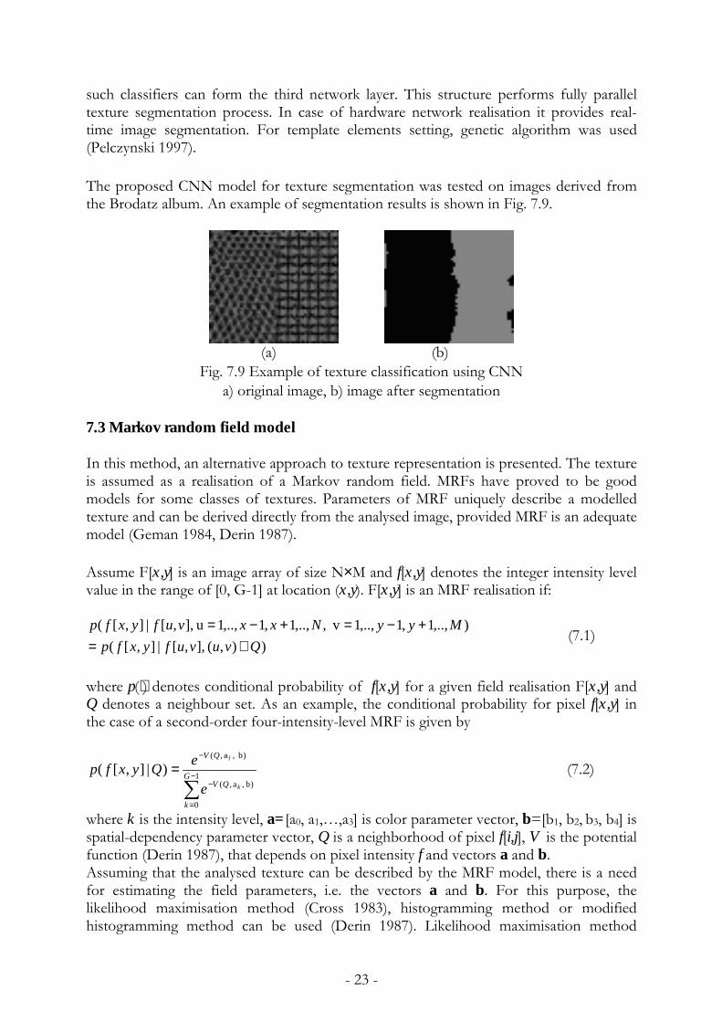
7.3 Markov random field model

In this method, an alternative approach to texture representation is presented. The textureis assumed as a realisation of a Markov random field. MRFs have proved to be goodmodels for some classes of textures. Parameters of MRF uniquely describe a modelledtexture and can be derived directly from the analysed image, provided MRF is an adequatemodel (Geman 1984, Derin 1987).

Assume F[x,y] is an image array of size N×M and f[x,y] denotes the integer intensity levelvalue in the range of [0, G-1] at location (x,y). F[x,y] is an MRF realisation if:

)),( ],,[|],[(),..,1,1,..,1 v,,..,1,1,..,1u ],,[|],[(

QvuvufyxfpMyyNxxvufyxfp

∈=+−=+−=

(7.1)

where p(⋅) denotes conditional probability of f[x,y] for a given field realisation F[x,y] andQ denotes a neighbour set. As an example, the conditional probability for pixel f[x,y] inthe case of a second-order four-intensity-level MRF is given by

)|],[( 1

0

)b ,a ,(

)b ,a ,( f

∑−

=

−

−

= G

k

QV

QV

ke

eQyxfp (7.2)

where k is the intensity level, a=[a0, a1,…,a3] is color parameter vector, b=[b1, b2, b3, b4] isspatial-dependency parameter vector, Q is a neighborhood of pixel f[i,j], V is the potentialfunction (Derin 1987), that depends on pixel intensity f and vectors a and b.Assuming that the analysed texture can be described by the MRF model, there is a needfor estimating the field parameters, i.e. the vectors a and b. For this purpose, thelikelihood maximisation method (Cross 1983), histogramming method or modifiedhistogramming method can be used (Derin 1987). Likelihood maximisation method

- 24 -

provides high estimation accuracy but requires long computation time. Thehistogramming method is fast but less accurate, especially when used for estimation ofspatial-dependency vector parameter b. The modified histogramming method is acombination of likelihood maximisation and histogramming, where estimation of MRFparameters is performed independently for vectors a and b (Strzelecki 1997).

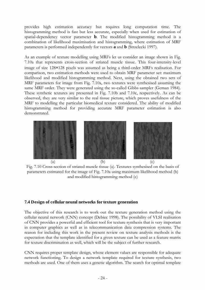
As an example of texture modelling using MRFs let us consider an image shown in Fig.7.10a that represents cross-section of striated muscle tissue. This four-intensity-levelimage of size 128×128 pixels was assumed as being a third-order MRFs realisation. Forcomparison, two estimation methods were used to obtain MRF parameter set: maximumlikelihood and modified histogramming method. Next, using the obtained two sets ofMRF parameters for image from Fig. 7.10a, two textures were synthesised assuming thesame MRF order. They were generated using the so-called Gibbs sampler (Geman 1984).These synthetic textures are presented in Fig. 7.10b and 7.10c, respectively. As can beobserved, they are very similar to the real tissue picture, which proves usefulness of theMRF to modelling the particular biomedical texture considered. The ability of modifiedhistogramming method for providing accurate MRF parameter estimation is alsodemonstrated.

(a) (b) (c)

Fig. 7.10 Cross-section of striated muscle tissue (a). Textures synthesised on the basis ofparameters estimated for the image of Fig. 7.10a using maximum likelihood method (b)

and modified histogramming method (c)

7.4 Design of cellular neural networks for texture generation

The objective of this research is to work out the texture generation method using thecellular neural network (CNN) concept (Debiec 1998). The possibility of VLSI realisationof CNN provides a powerful and efficient tool for texture synthesis that is very importantin computer graphics as well as in telecommunication data compression systems. Thereason for including this work in the present review on texture analysis methods is theexpectation that the template identified for a given texture can be used as a feature matrixfor texture discrimination as well, which will be the subject of further research.

CNN requires proper template design, whose element values are responsible for adequatenetwork functioning. To design a network template required for texture synthesis, twomethods are used. One of them uses a genetic algorithm. The search for optimal template

- 25 -

requires modification of network template population, which elements were randomlygenerated. The template is designed based on minimisation of chosen fitness function.The generation procedure starts from white noise image with small variance. This initialimage is processed by the CNN for each template from its population. Next, for thetexture image obtained at the network outputs, the values of statistical features arecalculated and compared with values required. The ‘best fitted’ templates are chosen asparent templates for the next populations, which are created using reproduction,crossover and mutation. These operations work on binary strings used for coding oftemplate element values. The learning procedure is stopped when the fitness functionvalue reaches a given value.

Table 1. Examples of CNN-generated textures for different number ofstatistical features used for their description

Texture 1

2.41 -2.25 -1.03A = -0.20 3.12 3.17 -0.96 2.83 0.18Feature value:required obtainedVAR = 0.85 VAR = 0.85

Texture 2:

0.39 -0.08 0.33 A = -1.13 -0.19 1.47 0.54 1.73 -2.63Feature values:required obtainedVAR = 0.50 VAR = 0.55EX = 0.00 EX = 0.00

Texture 3:

0.22 -2.07 0.81A = 2.94 0.20 -2.75 -2.30 -0.18 0.18Feature values:required obtainedVARx = 0.20 VARx = 0.33VARy = 0.40 VARy = 0.38EX = -0.42 EX = -0.30

(A – template matrix, VAR – variance, EX – expected value, VARx, VARy – variances ofmarginal distributions)

Experimental results are presented in Table 1. Texture representation using one featureonly (for example variance) provides good results in terms of CNN template obtained.The texture generated using this template has the variance value the same, as it wasrequired. Unfortunately, the increase of texture features causes less accurate results,increasing computational time significantly.

The obtained textures are very simple and they look binary. For grey-level texturegeneration, the alternative method was used. In this method, the CNN used for texturegeneration emulates an autoregressive FIR filter. To provide network stability, the initialimage (white noise) and generated texture image are transformed such that they possessnegative amplitude spectrum and phase spectrum equal to zero. The objective of templatedesign process is to obtain a stable CNN that generates a texture with the same amplitudespectrum as an original image (in terms of mean-square error).

- 26 -

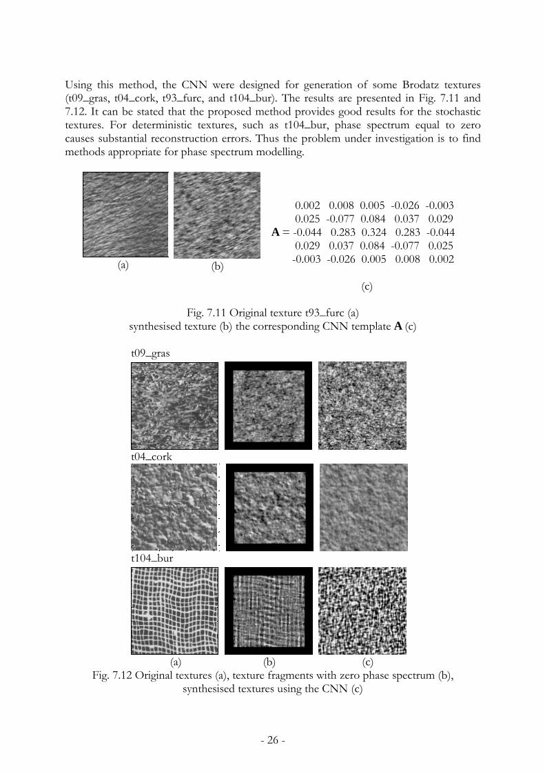
Using this method, the CNN were designed for generation of some Brodatz textures(t09_gras, t04_cork, t93_furc, and t104_bur). The results are presented in Fig. 7.11 and7.12. It can be stated that the proposed method provides good results for the stochastictextures. For deterministic textures, such as t104_bur, phase spectrum equal to zerocauses substantial reconstruction errors. Thus the problem under investigation is to findmethods appropriate for phase spectrum modelling.

(a) (b)

0.002 0.008 0.005 -0.026 -0.003 0.025 -0.077 0.084 0.037 0.029A = -0.044 0.283 0.324 0.283 -0.044 0.029 0.037 0.084 -0.077 0.025 -0.003 -0.026 0.005 0.008 0.002

(c)

Fig. 7.11 Original texture t93_furc (a)synthesised texture (b) the corresponding CNN template A (c)

t09_gras

t04_cork

t104_bur

(a) (b) (c)

Fig. 7.12 Original textures (a), texture fragments with zero phase spectrum (b),synthesised textures using the CNN (c)

- 27 -

7.4 Radiographic texture analysis

Image analysis techniques for detection of changes in bone mineral density (BMD) areexamined in (Cichy 1997). The results are compared with BMD measured using dual-energy X-ray absorptiometry (DXA) method. X-ray patterns were registered in the sameconditions of exposure and chemical development. Additionally, a calibration phantomwas used to standardise the results. Radiogram patterns were digitised with a CCDcamera. The following texture parameters were computed: the mean of intensity, standarddeviation of intensity, skewness, kurtosis, energy, entropy and fractal dimension. Themean value, standard deviation and coefficient of linear correlation with BMD wereestimated for every parameter. Occurrence probability of intensity level is highlycorrelated with DXA-measured results. It seems that analysis of fractal dimension canadditionally enrich diagnostic knowledge about bone microarchitecture. Examples ofbone tissue X-ray images are presented in Fig. 13.

(a) (b) (c)Fig. 7.13 Sample X-ray images of bone tissue for different BMD coefficients

(a) - BMD=0.56, (b) - BMD=0.31, (c) - BMD=0.14.

8. Summary

The above review of texture analysis methods is by no means exhaustive. Further librarysearch and numerical investigation are needed to make the material collected morecomplete. Investigation of actual MR image properties would make the search foradequate texture analysis methods better focused.

- 28 -

Acknowledgment

The authors wish to thank Mr Piotr Cichy, Mr Piotr Debiec and Mr Pawel Pelczynski forproviding figures included in Chapter 7, respectively Fig. 13; Figs 6, 7, 11, 12; and Figs 4,5, 8, 9.

References

1965A. Papoulis, Probability, Random Variables and Stochastic Processes, McGraw-Hill, 1965.

1966P. Brodatz, Textures - A Photographic Album for Artists and Designers, Dover, 1966.

1975B. Julesz, “Experiments in the Visual Perception of Texture”, Scientific American, 232, 4,1975, 34-43.1976J. Weszka, C. Deya and A. Rosenfeld, “A Comparative Study of Texture Measures forTerrain Classification”, IEEE Trans. System, Man and Cybernetics, 6, 269-285, 1976.

1977O. Mitchell, C. Myers and W. Boyne, “A Max-Min Measure for Image Texture Analysis”,IEEE Trans. Computers, 408-414, 1977.

1979R. Haralick, “Statistical and Structural Approaches to Texture”, Proc. IEEE, 67, 5, 786-804, 1979.P. Chen and T. Pavlidis, “Segmentation by Texture Using a Co-Occurrence Matrix and aSplit-and Merge Algorithm”, CGIP, 10, 1979, 172-182.

1980A. Rosenfeld and J. Weszka, “Picture Recognition” in Digital Pattern Recognition, K. Fu(Ed.), Springer-Verlag, 135-166, 1980.

1981M. Hassner and J. Sklansky, “The Use of Markov Random Fields as Model s of Texture”,Image Modelling, A. Rosenfeld (Ed.), Academic Press, 1981, 185-198.H. Niemann, Pattern Analysis, Springer-Verlag, 1981.

1982A. Rosenfeld and A. Kak, Digital Picture Processing, vol. 1, Academic Press, 1982.J. Serra, Image Analysis and Mathematical Morphology, Academic Press, 1982.

- 29 -

1983G. Cross and A. Jain, “Markov Random Field Texture Models”, IEEE Trans. PatternAnalysis and Machine Intelligence, 5, 1, 25-39, 1983.G. Lowitz, “Can a Local Histogram Really Map Texture Information?”, Pattern Recognition,16, 2, 1983, 141-147.

1984S. Geman and D. Geman, “Stochastic Relaxation, Gibbs Distribution and the BayesianRestoration of Images”, IEEE Trans. Pattern Analysis and Machine Intelligence, 6, 11, 1984,721-741.A. Pentland, “Fractal-Based Description of Natural Scenes”, IEEE Trans. Pattern Analysisand Machine Intelligence, 6, 6, 661-674, 1984.

1985R. Chellappa and S. Chatterjee, “Classification of Textures Using Gaussian MarkovRandom Fields”, IEEE Trans. Acoustic, Speech and Signal Processing, 33, 4, 959-963, 1985.J. Daugman, “Uncertainty Relation for Resolution in Space, Spatial Frequency andOrientation Optimised by Two-Dimensional Visual Cortical Filters”, Journal of the OpticalSociety of America, 2, 1160-1169, 1985.M. Levine, Vision in Man and Machine, McGraw-Hill, 1985.

1987A. Blake and A. Zisserman, Visual Reconstruction, The MIT Press, 1987.H. Derin and H. Elliot, “Modeling and Segmentation of Noisy and Textured ImagesUsing Gibbs Random Fields”, IEEE Trans. Pattern Analysis and Machine Intelligence, 9, 1, 39-55, 1987.

1989M. Amadasun and R. King, “Textural Features Corresponding to Textural Properties”,IEEE Transactions on System, Man Cybernetics, 19, 5, 1989, 1264-1274.C-C. Chen, J. Daponte and M. Fox, “Fractal Feature Analysis and Classification inMedical Imaging”, IEEE Trans. Medical Imaging, 8, 2, 1990, 133-142.L. Cohen, “Time-Frequency Distributions – A Review”, Proceedings IEEE, 77, 7, 1989,941-981.P. Cohen, C. LeDinh and V. Lacasse, “Classification of Natural Textures by Means ofTwo-Dimensional Orthogonal Masks”, IEEE Trans. Acoustics, Speech and Signal Processing,37, 1, 1989, 125-128.J. Hsiao and A. Sawchuk, “Supervised Textured Image Segmentation Using FeatureSmoothing and Probabilistic Relaxation Techniques”, IEEE Trans. Pattern Analysis andMachine Intelligence, 11, 12, 1989, 1279-1292.J. Hsiao and A. Sawchuk, “Supervised Textured Image Segmentation Using FeatureSmoothing and Probabilistic Relaxation Techniques”, CVGIP, 48, 1989, 1-20.A. Jain, Fundamentals of Digital Image Processing, Prentice Hall, 1989.S. Mallat, “Multifrequency Channel Decomposition of Images and Wavelet Models”,IEEE Trans. Acoustic, Speech and Signal Processing, 37, 12, 1989, 2091-2110.

- 30 -

1990L. Alparone, F. Argenti and G. Benelli, “Fast Calculation of Co-Occurrence MatrixParameters For Image Segmentation”, Electronics Letters, 26, 1, 1990, 23-24.F. Argenti, L. Alparone and G. Benelli, “Fast Algorithms for Texture Analysis Using Co-Occurrence Matrices”, IEE Proceedings, 137, F, 6, 1990, 443-448.A. Bovik, M. Clark and W. Giesler, “Multichannel Texture Analysis Using LocalisedSpatial Filters”, IEEE Trans. Pattern Analysis and Machine Intelligence, 12, 1990, 55-73.K. Fukunaga, Introduction to Statistical Pattern Recognition, Academic Press, 1990R. Hecht-Nielsen, Neurocomputing, Addison-Wesley, 1990.T. Reed and H. Wechsler, “Segmentation of Textured Images and Gestalt OrganizationUsing Spatial/Spatial-Frequency Representations”, IEEE Trans. Pattern Analysis andMachine Intelligence, 12, 1,1990,1-12.M. Unser and M. Eden, “Nonlinear Operators for Improving Texture SegmentationBased on Features Extracted by Spatial Filtering”, IEEE Trans. System Man Cybernetics, 20,4, 1990, 804-815.

1991F. Cohen, Z. Fan and M. Patel, “Classification of Rotated and Scaled Textured ImagesUsing Gaussian Markov Random Field Models”, IEEE Trans. Pattern Analysis and MachineIntelligence, 13, 2, 192-202, 1991.A. Jain and F. Farrokhnia, “Unsupervised Texture Segmentation Using Gabor Filters”,Pattern Recognition, 24, 12, 1991, 1167-1186.B. Manjunath and R. Chellappa, “Unsupervised Texture Segmentation Using MarkovRandom Fields”, IEEE Trans. Pattern Analysis and Machine Intelligence, 13, 5, 478-482, 1991.W. Pratt, Digital Image Processing, Wiley, 1991.

1992R. Gonzalez and R. Woods, Digital Image Processing, Addison-Wesley, 1992.J. Mao and A. Jain, “Texture Classification and Segmentation Using MulriresolutionSimultaneous Autoregressive Models”, Pattern Recognition, 25, 2, 1992, 173-188.H-O. Peitgen, H. Jurgens and D. Saupe, Chaos and Fractals, Springer-Verlag, 1992.

1993S. Chen, J. Keller and R. Crownover, “On the Calculation of Fractal Features fromImages”, IEEE Trans. Pattern Analysis and Machine Intelligence, 15, 10, 1993, 1087-1090.A. Laine and J. Fan, “Texture Classification by Wavelet Packet Signatures”, IEEE Trans.Pattern Analysis and Machine Intelligence, 15, 11, 1993, 1186-1191.R. Lerski, K. Straughan, L. Shad, D. Boyce, S. Bluml, and I. Zuna, “MR Image TextureAnalysis – An Approach to Tissue Characterisation”, Magnetic Resonance Imaging, 11, 1993,873-887.

1994M. Bello, “A Combined Markov Random Field and Wave-Packet Transform-BasedApproach for Image Segmentation”, IEEE Trans. Image Processing, 3, 6, 1994, 834-846.J. Bigun and J. du Buf, “N-folded Symmetries by Complex Moments in Gabor Space andTheir Application to Unsupervised Texture Segmentation”, IEEE Trans. Pattern Analysisand Machine Intelligence, 16, 1, 1994, 80-87.

- 31 -

Y. Chen and E. Dougherty, “Grey-Scale Morphological Granulometric TextureClassification”, Optical Engineering, 33, 8, 1994, 2713-2722.M-P. Dubuisson and R. Dubes, “Efficacy of Fractal Features in Segmenting Images ofNatural Textures”, Pattern Recognition Letters, 15, 1994, 419-431.D. Dunn, W. Higgins and J. Wakeley, “Texture Segmentation Using 2-D GaborElementary Functions”, IEEE Trans. Pattern Analysis and Machine Intelligence, 16, 2, 1994,130-149.M. Gurelli and L. Onural, “On a Parameter Estimation Method for Gibbs-MarkovFields”, IEEE Trans. Pattern Analysis and Machine Intelligence, 16, 4, 1994, 424-430.Y. Hu and T. Dennis, “Textured Image Segmentation by Context Enhanced Clustering”,IEE Proc.-Visual Image and Signal Processing, 141, 6, 1994, 413-421.R. Jennane and R. Harba, “Fractional Brownian Motion: A Model for Image Texture”,SIGNAL PROCESSING VII: Theories and Applications, M. Holt et al. (Eds.), 1994, 1389-1392.P. Pelczynski and P. Strumillo, “Artificial Neural Network Model for Feature Extractionand Segmentation of Visual Textures”, 17-th National Conf. Circuit Theory and ElectronicSystems, Wroclaw, Poland, 1994, 489-494.N. Sarkar and B. Chaudhuri, ”An Efficient Differential Box-Counting Approach toCompute Fractal Dimension of Image”, IEEE Trans. System Man Cybernetics, 24, 1, 115-120.L. Sukissian, S. Kollias and Y. Boutalis, “Adaptive Classification of Textured ImagesUsing Linear Prediction and Neural Networks”, Signal Processing, 36, 1994, 209-232.H. Yin and N. Allinson, “Unsupervised Segmentation of textured Images Using aHiererchical Neural Structure”, Electronics Letters, 30, 22, 1994, 1842-1843.

1995M. Augusteijn, “Texture Segmentation and Classification Using Neural NetworkTechnology”, Applied Mathematics and Computer Science, 4, 1995, 353-370.B. Chaudhuri and N. Sarkar, “Texture Segmentation Using Fractal Dimension”, IEEETrans. Pattern Analysis and Machine Intelligence, 17, 1, 1995, 72-77.J-L. Chen and A. Kundu, “Unsupervised Texture Segmentation Using MultichannelDecomposition and Hidden Markov Models”, IEEE Trans. Image Processing, 4, 5, 1995,603-619.Y-Q. Chen, M. Nixon and D. Thomas, “Statistical Geometrical Features for TextureClassification”, Pattern Recognition, 28, 4, 1995, 537-552.D. Dunn and W. Higgins, “Optimal Gabor Filters for Texture Segmentation”, IEEETrans. Image Processing, 4, 7, 1995, 947-964.L. Kaplan and C-C. Kuo, “Texture Roughness Analysis and Synthesis via Extended Self-Similar (ESS) Model”, IEEE Trans. Pattern Analysis and Machine Intelligence, 17, 11, 1995,1043-1056.C. Kervrann and F. Heitz, “A Markov Random Field Model-Based Approach toUnsupervised Texture Segmentation Using Local and Global Spatial Statistics”, IEEETrans. Image Processing, 4, 6, 1995, 856-862.D. Panjwani and G. Healey, “Markov Random Field Models for UnsupervisedSegmentation of Textured Color Images”, IEEE Trans. Pattern Analysis and MachineIntelligence, 17, 11, 1995, 939-954.

- 32 -

B. Povlow and S. Dunn, “Texture Classification Using Noncausal Hidden MarkovModels”, IEEE Trans. Pattern Analysis and Machine Intelligence, 17, 10, 1995, 1010-1014.M. Strzelecki, Segmentation of Textured Biomedical Images Using Neural Networks, PhD Thesis,Technical University of Łódź, Poland, 1995 (in Polish).A. Teuner, O. Pichler and B. Hosticks, “Unsupervised Texture Segmentation of ImagesUsing Tuned Matched Gabor Filters”, IEEE Trans. Image Processing, 4, 6, 1995, 863-870.S. Yhann and T. Young, “Boundary Localisation in Texture Segmentation”, IEEE Trans.Image Processing, 4, 6, 1995, 849-856.

1996M. Brady and Z-Y. Xie, “Feature Selection for Texture Segmentation”, in Advances inImage Understanding, K. Bowyer and N. Ahuja (Eds.), IEEE Computer Society Press, 1996.S. Doh and R-H. Pang, “Segmentation of Statistical Texture Images Using the MetricSpace Theory”, Signal Processing, 53, 1996, 27-34.A. Jain and K. Karu, “Learning Texture Discrimination Masks”, IEEE Trans. PatternAnalysis and Machine Intelligence, 18, 2, 1996, 195-205.V. Kovalev and M. Petrou, “Multidimensional Co-Occurrence Matrices for ObjectRecognition and Matching”, GMIP, 58, 3, 1996, 187-197.R. Porter and N. Canagarajah, “A Robust Automatic Clustering Scheme for ImageSegmentation Using Wavelets”, IEEE Trans. Image Processing, 5, 4, 1996, 662-665.A. Speis and G. Healey, “An Analytical and Experimental Study of the Performance ofMarkov Random Fields Applied to Textured Images Using Small Samples”, IEEE Trans.Image Processing, 5, 3, 1996, 447-458.G. Strang and T. Nguyen, Wavelets and Filter Banks, Wellesley-Cambridge Press, 1996.

1997P. Cichy, A. Materka and J. Tuliszkiewicz, “Computerised Analysis of X-ray Images ForEarly Detection of Osteoporotic Changes in the Bone”, Proc. Conf. Information Technology inMedicine TIM ‘97, Jaszowiec, Poland, 53-61, 1997 (in Polish).K. Delibasis, P. Undrill and G. Cameron, “Designing Texture Filters with GeneticAlgorithms: An Application to Medical Images”, Signal Processing, 57, 1997, 19-33.W-K. Lam and C-K. Li, “Rotated Texture Classification by Improved IterativeMorphological Decomposition”, IEE Proc. – Visual Image Signal Processing, 144, 3, 1997,171-179.S. Krishnamachari and R. Chellappa, “Multiresolution Gauss-Markov Random FieldModels for Texture Segmentation”, IEEE Trans. Image Processing, 6, 2, 1997, 251-267.C. Lu, P. Chung and C. Chen, “Unsupervised Texture Segmentation via WaveletTransform”, Pattern Recognition, 30, 5, 729-742, 1997.P. Pelczynski, “Cellular Neural Network for Segmentation of Textured Images”, ImageProcessing & Communications, 3, No. 3-4, 1997, 3-8.R. Porter and N. Canagarajah, “Robust Rotation-Invariant Texture Classification:Wavelet, Gabor Filter and GMRF Based Schemes”, IEE Proc. – Visual Image SignalProcessing, 144, 3, 1997, 180-188.A. Sarkar, K. Sharma and R. Sonak, “A New Approach for Subset 2-D AR ModelIdentification for Describing Textures”, IEEE Trans. Image Processing, 6, 3, 1997, 407-413.

- 33 -

M. Strzelecki and A. Materka, “Markov Random Fields as Models of Textured BiomedicalImages”, Proc. 20th National Conf. Circuit Theory and Electronic Networks KTOiUE ’97,Kołobrzeg, Poland, 493-498, 1997.

1998P. Andrey and P. Tarroux, “Unsupervised Segmentation of Markov Random FieldModelled Textured Images Using Selectionists Relaxation”, IEEE Trans. Pattern Analysisand Machine Intelligence, 20, 3, 1998, 252-262.J. Bennett and A. Khotanzad, “Multispectral Random Field Models for Synthesis andAnalysis of Color Images”, IEEE Trans. Pattern Analysis and Machine Intelligence, 20, 1, 1998,327-332.P. Debiec, “Design of cellular neural networks for textured image synthesis”, ZeszytyNaukowe Elektronika, 3, 1998, pp. (in Polish).K. Valkealathi and E. Oja, “Reduced Multidimensional Co-Occurrence Histograms inTexture Classification”, IEEE Trans. Pattern Analysis and Machine Intelligence, 20, 1, 1998,90-94.L. Bruzzone, F. Roli and S. Serpico, “Structured Neural Networks for SignalClassification”, Signal Processing, 64, 1998, 271-290.