TEXTO PARA DISCUSSÃO N° 211

INCREASING RETURNS TO SCALE AND INTERNATIONAL DIFFUSION OF TECHNOLOGY: AN EMPIRICAL STUDY FOR BRAZIL (1976-2000)

Francisco Horácio P. Oliveira

Frederico G. Jayme Jr Mauro B. Lemos

Julho de 2003

Ficha catalográfica

330.34(81) O48i 2003

Oliveira, Francisco Horácio P. Increasing returns to scale and international diffusion of technology: an empirical study for Brazil (1976-2000) / por Francisco Horácio P. Oliveira, Frederico G. Jayme Jr., Mauro B. Lemos. - Belo Horizonte: UFMG/Cedeplar, 2003.

25p. (Texto para discussão ; 211) 1. Desenvolvimento econômico. 2. Inovações tecnológicas. 3.

Produtividade industrial – Brasil – Modelos econometricos. 4. Brasil – Condições econômicas – 1976-2000. I. Jayme Jr., Frederico G. II. Lemos, Mauro B. III. Universidade Federal de Minas Gerais. Centro de Desenvolvimento e Planejamento Regional. IV. Título. V. Série.

CDU

2

UNIVERSIDADE FEDERAL DE MINAS GERAIS FACULDADE DE CIÊNCIAS ECONÔMICAS

CENTRO DE DESENVOLVIMENTO E PLANEJAMENTO REGIONAL

INCREASING RETURNS TO SCALE AND INTERNATIONAL DIFFUSION OF TECHNOLOGY: AN EMPIRICAL STUDY FOR BRAZIL (1976-2000)*

Francisco Horácio P. Oliveira Adjunct Professor at the Economics Department, Federal University of Minas Gerais.

Rua Curitiba, 832, 7°andar, sala 701 / Belo Horizonte, MG, Brazil 30170-120. (chico@cedeplar.ufmg.br)

Frederico G. Jayme Jr

Associate Professor at the Economics Department, Federal University of Minas Gerais. (gonzaga@cedeplar.ufmg.br).

Mauro B. Lemos

Professor at the Economics Department, Federal University of Minas Gerais. (mbl@cedeplar.ufmg.br).

CEDEPLAR/FACE/UFMG BELO HORIZONTE

2003

* The authors are grateful to the valuable comments by Professor Gilberto Tadeu Lima, from University of São Paulo (USP).

The usual disclaimers apply.

3

SUMÁRIO INTRODUCTION................................................................................................................................... 6 1.THEORETICAL DETERMINANTS OF ECONOMIC GROWTH: KALDORIAN AND

SCHUMPETERIAN CONTRIBUTIONS .......................................................................................... 6 2. THE THEORETICAL MODEL ......................................................................................................... 8 3. MATERIAL AND METHODS .......................................................................................................... 9 4. EMPIRICAL EVIDENCES OF SHORT-TERM AND LONG-TERM TRAJECTORIES .............. 11 4.1 Test for the Output Equation ........................................................................................................... 11 4.2. Test for the Productivity Equation ................................................................................................. 16 5. CONCLUSIONS............................................................................................................................... 21 REFERENCES...................................................................................................................................... 24

4

ABSTRACT

This article aims at exploring the empirical evidence regarding the effects of increasing returns to scale and international technological diffusion on the Brazilian manufacturing industry. Our departure point is a Kaldorian-type theoretical model that provides not only the positive effects of scale but also of diffusion on industrial performance. We use Vector Auto Regressive (VAR) for testing the model. VAR will estimate the coefficients related to industrial output, labor productivity, exports and the technological gap between the United States and Brazil. This technique also provides simulations for the short-term and long-term trajectories under exogenous shocks. The observations are on a three-month period basis and the sampling period runs from the second half of 1976 to the second half of 2000. The conclusion highlights both evidences of increasing returns on the Brazilian industry that faces, however, some structural constraints. Besides, the model also reveals Brazil’s difficulties to catch up. Key Words: technological gap; increasing returns to scale, economic growth. JEL: O0, C1 e C22. RESUMO

O artigo apresenta evidências empíricas para a influência da hipótese de retornos crescentes de escala e de difusão internacional de tecnologia sobre o comportamento da taxa de crescimento do produto industrial brasileiro. Partindo de um modelo teórico que concilia essas duas hipóteses, a metodologia do trabalho está centrada na utilização de VAR (Vetores Auto Regressivos) a fim de estimar coeficientes que relacionem produção industrial brasileira, produtividade do trabalho, exportações e hiato tecnológico entre Brasil e EUA. As observações são trimestrais, e o período das amostras estende-se do 2º trimestre de 1976 até o 2º trimestre de 2000. As conclusões sinalizam para o fato de que, apesar da evidência de retornos crescentes para o período considerado, existem limitações estruturais da economia brasileira que impedem ganhos permanentes na produtividade do trabalho a partir do learning by doing. Associado a isso, o Brasil não realiza o processo de catching up, ou seja, as evidências não confirmam o fato de que nossa economia tenha a capacidade de participar do processo de difusão internacional de tecnologia. Palavras-Chave: Hiato tecnológico, Retornos Crescentes de Escala, Crescimento Econômico JEL: O0, C1 e C22.

5

INTRODUCTION

Our aim in this paper is to incorporate new empirical evidence on the determinants of the Brazilian industrial performance. More specifically, we attempt to test the empirical relevance of the hypotheses of increasing returns to scale and technological absorption for determining output growth of the Brazilian manufacturing industry. We use time series of industrial output, industrial labor productivity, exports, and the American industrial labor productivity. They are based on quarterly observations extending from the 2nd quarter of 1976 to the 2nd quarter of 2000. Our theoretical approach tries to integrate the Kaldorian literature on economic growth with the Schumpeterian literature on technological innovation and diffusion.

In addition to the introduction, the paper has five sections. Section 1 is a brief review of the theoretical developments based on Kaldor’s work on economic growth (Kaldor, 1966) and the literature on catching up. We argue that these approaches are complementary for explaining economic growth rate differentials both between distinct time periods within a country and among countries in a time span. Section 2 presents a growth model derived from Dixon and Thirlwall (1975) and its extended version provided by Higachi, Canuto, and Porcile (1999). Section 3 shows the database and the methodology for the empirical estimates. Section 4 presents the main results, which includes tests for the long-run relationship among industrial output (dependent variable), productivity, and exports. Finally, the last section sums up the major results and the concluding remarks. 1.THEORETICAL DETERMINANTS OF ECONOMIC GROWTH: KALDORIAN AND

SCHUMPETERIAN CONTRIBUTIONS

Kaldor (1966) introduced the role of increasing returns to scale in explaining the growth rate differentials among countries. His original model assumes growth as a result of the interaction between manufacturing industry, subject to increasing returns to scale, and agriculture, a backward sector subject to decreasing returns to scale due to excess labor force1. Insofar as the industrial sector increases its production, labor productivity also increases due to increasing returns, which imply a rise in the worker’s real wage. Such a wage increase will attract labor from the backward sector, which will benefit from the resulting reduction of the excess labor supply by productivity increases. Accordingly, increased labor stock with higher wages in the industrial sector will lead to additional rise in production, restarting the growth process. Thus, the economic growth of a country is led by a set of interactions in which the industrial sector is taken as the “growth engine”. Indeed, labor demand increases in industrial sector pulls productivity in all sectors of the economy. (McCombie & Thirlwall, 1994)

Such a process of continuous labor migration from the backward sector to industry engenders the “domestic market” of a country, based on increasing size of the industrial labor force and its real wages and the inter-sectoral demand-supply linkages. For this reason, according to Kaldor (1966), the internal market constitutes the main component of final demand in the intermediate stages of

1 Such hypothesis could already be found in the literature of the “dual models” discussed by Lewis (1969).

6

development, due to interactions between internal consumption and investment. When the demand expansion via increased domestic market is exhausted, exports become the major component of expanding final demand. Hence, the country’s foreign trade performance becomes crucial for sustained high growth rates. Kaldor’s emphasis on exports as the major component of final demand has led other authors to formalize Kaldorian ideas by using the hypothesis that growth is “led by exports”. Dixon & Thirlwall (1975) used the “Harrod’s foreign trade multiplier”, showed that growth rates are determined by the growth rate of exports and income-elasticity of the demand for exports.

Therefore, the leading component of final demand to growth varies according to a country’s development stage. As long as growth in developed mature countries is led by exports, in developing countries it is led by domestic market. This is the result of interactions between the industrial sector and the traditional one (Thirlwall, 1987; Mccombie, 1983). In other words, the major demand component in backward countries is not that of exports but that of domestic consumption and investment resulting from expansion of the industrial sector. Exports become a key component of demand when industrialization is already consolidated and income per capita of the primary sector is equal to that of the industrial sector. This fact characterizes what Kaldor called “economic maturity”.

The second hypothesis to be tested is known as the “catching up hypothesis” (Abramovitz, 1986). Its theoretical background can be traced back to Schumpeter (1933, 1943). The country’s technological progress stems from the interaction between two kinds of firms: the innovative firms, responsible for introducing technological innovations in the economy and the imitative ones, responsible for the diffusion of innovations throughout the economic system based on their activities of “technological imitation”. More specifically, the catching up models derive from an extension of the Schumpeterian argument for the diffusion of the world technological progress.

According to these models, countries can be divided into two groups. The first one is formed by “leading countries”, which are responsible for the frontier of the scientific knowledge and hence responsible for the major worldwide technological innovations. The second group are the “followers”, which do not possess scientific basis able to improve the knowledge frontier but which can lever up technological progress based on two distinct sources. The first (which is centered on the international diffusion of technology) is the absorption of innovation developed in the leading countries; and the second is the development of innovation based on improvements of the technological progress achieved by the leading countries – which characterizes “opportunity windows”. The major question for the following countries is that both possibilities of technological catching up involve relative costs smaller than those costs related to innovation for the leading countries (Perez & Soete, 1988). If followers can manage to efficiently absorb new technologies and improve them, it is possible that they can sustain a growth rate of labor productivity (a proxy for technological progress) above those rates for the leading countries.

Thus, the essence of the catching up hypothesis is the following (Fagerberg, 1988a, 1988b): the greater the technological gap between leading and backward countries, the greater the potential for technological progress of the followers, provided that they possesses the necessary “social capability” to absorb and improve the international technology diffusion with leading countries (Abramovitz, 1986). If these countries efficiently absorb technologies from the leading countries, the greater gap from the advanced countries the greater their productivity growth. In this way, catching up occurs

7

when a backward country is able to sustain over time a technological progress higher than that of the leading countries, due to a significant efficiency in absorbing technologies. However, technological gap is not a sufficient condition for catching up. A series of socioeconomic characteristics, allowing the backward countries to obtain “advantages from the gap”, is needed. Such characteristics are related to the scientific and educational infrastructure of a country, the magnitude of R&D, labor force capabilities, among others. These characteristics constitute the National Innovation System (NIS) of a country. The more its NIS capabilities in relation to the “mature countries”, the more chances a country can have in achieving catching up (Freeman, 1995; Nelson, 1993; Albuquerque, 1999).

In light of the aforesaid reasons, the next section will briefly discuss a theoretical model that joins the hypotheses of increasing returns to scale and catching up. Furthermore, we will specify VAR (Vector Auto Regressive) equation for estimating the model. 2. THE THEORETICAL MODEL

The theoretical model is based on the Dixon-Thirlwall representation of increasing returns to scale. Higachi, Canuto & Porcile (1999) included technological diffusion into the original model according to Fagerberg’s catching up model (1988b). The extended model can be described as follows:

iii xrg εα += (1)

( )zrrx s

n

sss γη +

= log (2)

( )zrrx n

s

nnn γη +

= log (3)

nnnn gr λβ += (4)

)/( δµλβ G

ssss Gegr −++= (5)

in which:

gi = the growth rate of output of country i (s = south, n = north); ri = the growth rate of labor productivity of country i; xi = the exports growth rate of country i; z = the income growth rate of foreign market; G = log (rn / rs) = the technological gap.

8

The model comprises two countries – the north and the south. The north transfers technology

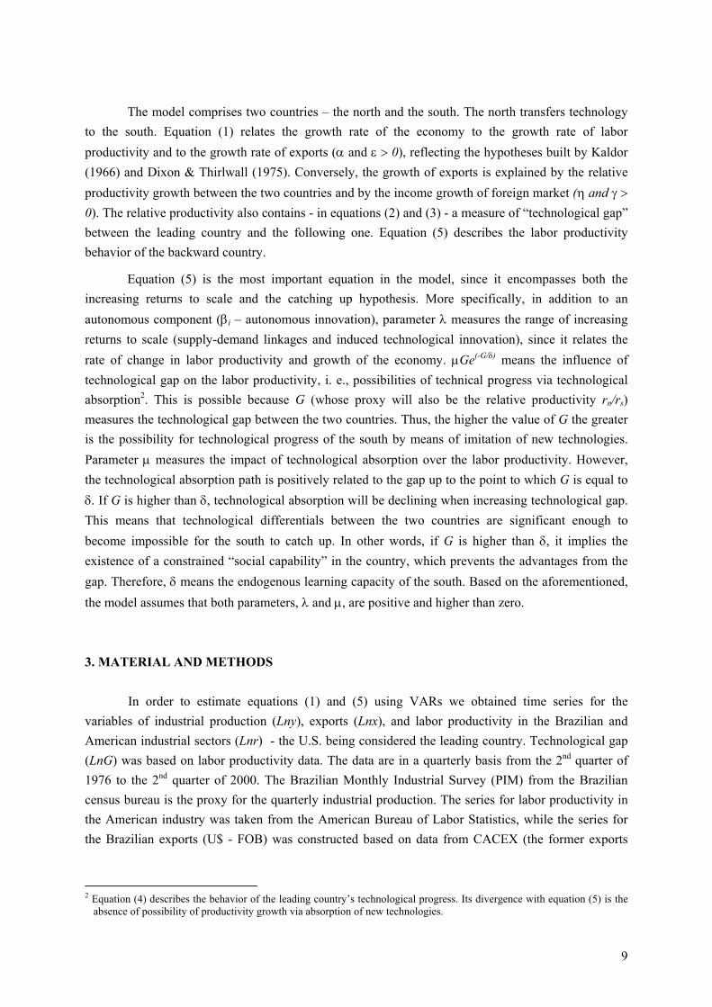
to the south. Equation (1) relates the growth rate of the economy to the growth rate of labor productivity and to the growth rate of exports (α and ε > 0), reflecting the hypotheses built by Kaldor (1966) and Dixon & Thirlwall (1975). Conversely, the growth of exports is explained by the relative productivity growth between the two countries and by the income growth of foreign market (η and γ > 0). The relative productivity also contains - in equations (2) and (3) - a measure of “technological gap” between the leading country and the following one. Equation (5) describes the labor productivity behavior of the backward country.

Equation (5) is the most important equation in the model, since it encompasses both the increasing returns to scale and the catching up hypothesis. More specifically, in addition to an autonomous component (βi – autonomous innovation), parameter λ measures the range of increasing returns to scale (supply-demand linkages and induced technological innovation), since it relates the rate of change in labor productivity and growth of the economy. µGe(-G/δ) means the influence of technological gap on the labor productivity, i. e., possibilities of technical progress via technological absorption2. This is possible because G (whose proxy will also be the relative productivity rn/rs) measures the technological gap between the two countries. Thus, the higher the value of G the greater is the possibility for technological progress of the south by means of imitation of new technologies. Parameter µ measures the impact of technological absorption over the labor productivity. However, the technological absorption path is positively related to the gap up to the point to which G is equal to δ. If G is higher than δ, technological absorption will be declining when increasing technological gap. This means that technological differentials between the two countries are significant enough to become impossible for the south to catch up. In other words, if G is higher than δ, it implies the existence of a constrained “social capability” in the country, which prevents the advantages from the gap. Therefore, δ means the endogenous learning capacity of the south. Based on the aforementioned, the model assumes that both parameters, λ and µ, are positive and higher than zero. 3. MATERIAL AND METHODS

In order to estimate equations (1) and (5) using VARs we obtained time series for the variables of industrial production (Lny), exports (Lnx), and labor productivity in the Brazilian and American industrial sectors (Lnr) - the U.S. being considered the leading country. Technological gap (LnG) was based on labor productivity data. The data are in a quarterly basis from the 2nd quarter of 1976 to the 2nd quarter of 2000. The Brazilian Monthly Industrial Survey (PIM) from the Brazilian census bureau is the proxy for the quarterly industrial production. The series for labor productivity in the American industry was taken from the American Bureau of Labor Statistics, while the series for the Brazilian exports (U$ - FOB) was constructed based on data from CACEX (the former exports

2 Equation (4) describes the behavior of the leading country’s technological progress. Its divergence with equation (5) is the

absence of possibility of productivity growth via absorption of new technologies.

9

division of the Banco do Brasil) and from the databank of SECEX (the federal government’s secretariat for foreign trade).

We will estimate increasing returns to scale and technological absorption by using VAR and an Error Correction Model.3 Thus, we will carry out unit roots tests (ADF and Phillips-Perron) for the variables of equations (1) and (5) and, if the series are non-stationary, Johansen’s cointegration test whose results reveals the presence of cointegration and provide cointegrating parameters. The crucial point is that Johansen’s test is performed assuming that the time series behavior is described by the VARs and shows a cointegration relation expressed by a “mechanism of error correction” (Charemza & Deadman, 1997). Tables 1 and 2 show the Unit Root tests (ADF and Phillips-Perron) of the series at level and at the 1st difference.

TABLE 1 Unit Root Tests with intercept

Series (level and first difference)

SERIES ADF(2) ADF(3) ADF(4) PP(3) Ln y -1.74 -1.62 -1.97 -3.60 ∆Ln y -8.89 -5.05 -4.06 - Ln r 1.94 2.37 1.56 - ∆Ln r -9.63 -5.25 -3.9 - Ln x -1.99 -1.92 -1.48 - ∆Ln x -10.59 -4.45 -5.6 - Ln G -5.24 -4.34 -3.7 -7.92 ∆Ln G -8.1 -7.8 -7.3 -166.28

MacKinnon’s critical values for rejecting the null hypothesis of unit root: -3.5015 (1%), -2.8925 (5%), -2.5831 (10%).

Table 1 shows the results of ADF test with four differences (as suggested by AIC and SIC).

The equation estimated by the ADF test includes four differences so that they may generate a white noise. This table also shows the results of the Phillips-Perron test, taking three differences.

MacKinnon’s critical values show that the series for the output, labor productivity, and exports present unit root at level, but they are stationary at the 1st difference at 1%. Only the series for technological gap is stationary both at level and at the 1st difference.

A difference between the ADF test and the Phillips-Perron test as for the series for the product at level can be perceived. PP test indicates stationarity, while the ADF test – for all differences considered – indicates the existence of unit root. In accordance with Holden & Perman (1994), such differences may occur to the extent that PP test considers that the residues of the ADF estimated equation are not normal and follow an stochastic process MA (1). In case the statistics of the ADF do not indicate absence of normality of the residues, then the ADF test becomes preferable to the PP test.

3 A methodological description of cointegration, vector auto regression, and error correction model will not be presented

here. For a good discussion on the subject, see Holden & Perman (1994), Charemza and Deadman (1997), Hamilton (1994), Mills (1993), Enders (1995). A more in-depth discussion on the subject can be found in Maddala and Kim (1999), among others.

10

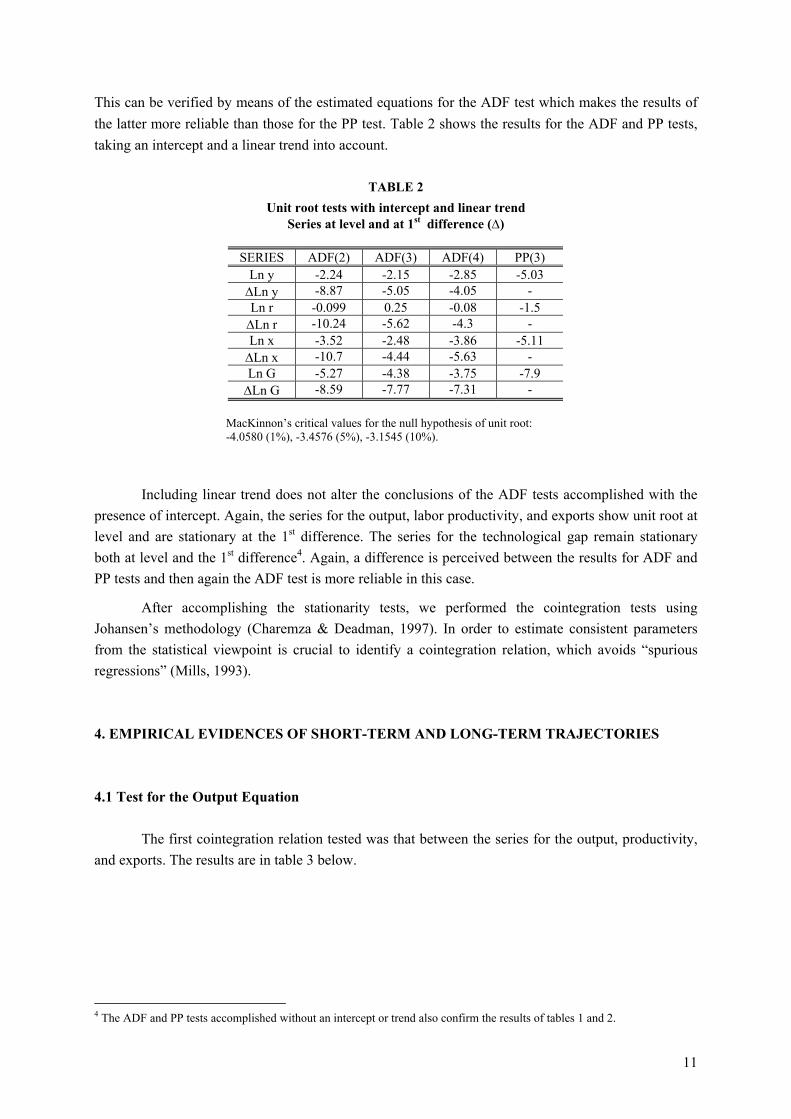
This can be verified by means of the estimated equations for the ADF test which makes the results of the latter more reliable than those for the PP test. Table 2 shows the results for the ADF and PP tests, taking an intercept and a linear trend into account.

TABLE 2

Unit root tests with intercept and linear trend Series at level and at 1st difference (∆)

SERIES ADF(2) ADF(3) ADF(4) PP(3)

Ln y -2.24 -2.15 -2.85 -5.03 ∆Ln y -8.87 -5.05 -4.05 - Ln r -0.099 0.25 -0.08 -1.5 ∆Ln r -10.24 -5.62 -4.3 - Ln x -3.52 -2.48 -3.86 -5.11 ∆Ln x -10.7 -4.44 -5.63 - Ln G -5.27 -4.38 -3.75 -7.9 ∆Ln G -8.59 -7.77 -7.31 -

MacKinnon’s critical values for the null hypothesis of unit root: -4.0580 (1%), -3.4576 (5%), -3.1545 (10%).

Including linear trend does not alter the conclusions of the ADF tests accomplished with the

presence of intercept. Again, the series for the output, labor productivity, and exports show unit root at level and are stationary at the 1st difference. The series for the technological gap remain stationary both at level and the 1st difference4. Again, a difference is perceived between the results for ADF and PP tests and then again the ADF test is more reliable in this case.

After accomplishing the stationarity tests, we performed the cointegration tests using Johansen’s methodology (Charemza & Deadman, 1997). In order to estimate consistent parameters from the statistical viewpoint is crucial to identify a cointegration relation, which avoids “spurious regressions” (Mills, 1993). 4. EMPIRICAL EVIDENCES OF SHORT-TERM AND LONG-TERM TRAJECTORIES 4.1 Test for the Output Equation

The first cointegration relation tested was that between the series for the output, productivity,

and exports. The results are in table 3 below.

4 The ADF and PP tests accomplished without an intercept or trend also confirm the results of tables 1 and 2.

11

TABLE 3 Johansen’s cointegration test and the number of cointegrating equations

Output, Productivity, Exports

Likelihood Ratio Critical value 5% significance

Critical Value 1% significance

Hypothesis (H0) – Number Cointegrating Equations

27.33617 24.31 29.75 Zero 10.96579 12.53 16.31 1 at most 0.858632 3.84 6.51 2 at most

The test equation does not show an intercept or linear trend and shows two successive differences for the variables.

The equation estimated did not assume an intercept or linear trend in the data. The first line of the table shows the test of the H0 hypothesis that there is no cointegration relation between the series. As the likelihood ratio estimated for Johansen’s test (27.33617) is higher then the critical values at 5% of significance, the H0 hypothesis is rejected, which means that there is a cointegration relation between those series. As for the cointegrating coefficients, the estimated value of the likelihood ratio in the second line is below the critical values. This leads to the rejection of the H0 hypothesis, i. e., there exists one cointegrating equation at most. Johansen’s test also provides cointegrating coefficients which are described in table 4 below:

TABLE 4 Cointegrating Coefficients for the relation between output,

productivity, and exports

Output Productivity Exports 0.839298 0.002172 0.310216

Normalized Cointegrated Coefficients

1 0,002588 0,369614

Statistics t - (-0.01742) (-130.005)

Equation (1) was the reference in which production behavior is explained by labor

productivity and exports. Thus, the estimated cointegrating coefficients endorse the theoretical reasoning, by positively relating production behavior to both labor productivity and exports. The table also shows no statistical significance of the productivity elasticity. Based on the value of the estimated statistics (-0.01742), the coefficient is not significant at the level of 10%. This fact cannot be ignored, since the relation between labor productivity and production is theoretically very important. In order to face this problem, we used Johansen’s test but with other specifications in the test equation and with higher successive differences. More specifically, the adjustment in the test took into account the hypothesis of one intercept in the cointegrating equation, a linear trend in the VARs, and successive differences in the order of 4.

However, the most important hypothesis assumed in the equation was that the labor productivity deviation could only have a positive impact on production one year after. As the

12

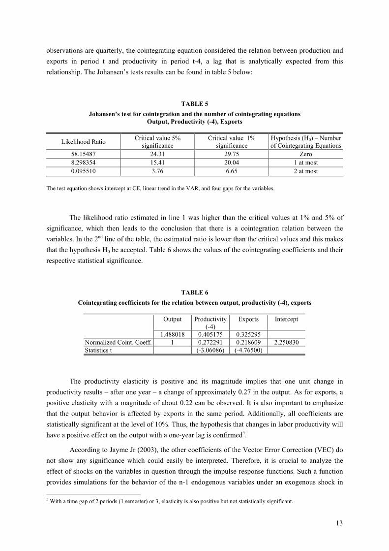
observations are quarterly, the cointegrating equation considered the relation between production and exports in period t and productivity in period t-4, a lag that is analytically expected from this relationship. The Johansen’s tests results can be found in table 5 below:

TABLE 5 Johansen’s test for cointegration and the number of cointegrating equations

Output, Productivity (-4), Exports

Likelihood Ratio Critical value 5% significance

Critical value 1% significance

Hypothesis (H0) – Number of Cointegrating Equations

58.15487 24.31 29.75 Zero 8.298354 15.41 20.04 1 at most 0.095510 3.76 6.65 2 at most

The test equation shows intercept at CE, linear trend in the VAR, and four gaps for the variables.

The likelihood ratio estimated in line 1 was higher than the critical values at 1% and 5% of significance, which then leads to the conclusion that there is a cointegration relation between the variables. In the 2nd line of the table, the estimated ratio is lower than the critical values and this makes that the hypothesis H0 be accepted. Table 6 shows the values of the cointegrating coefficients and their respective statistical significance.

TABLE 6 Cointegrating coefficients for the relation between output, productivity (-4), exports

Output Productivity

(-4) Exports Intercept

1.488018 0.405175 0.325295 Normalized Coint. Coeff. 1 0.272291 0.218609 2.250830 Statistics t (-3.06086) (-4.76500)

The productivity elasticity is positive and its magnitude implies that one unit change in productivity results – after one year – a change of approximately 0.27 in the output. As for exports, a positive elasticity with a magnitude of about 0.22 can be observed. It is also important to emphasize that the output behavior is affected by exports in the same period. Additionally, all coefficients are statistically significant at the level of 10%. Thus, the hypothesis that changes in labor productivity will have a positive effect on the output with a one-year lag is confirmed5.

According to Jayme Jr (2003), the other coefficients of the Vector Error Correction (VEC) do not show any significance which could easily be interpreted. Therefore, it is crucial to analyze the effect of shocks on the variables in question through the impulse-response functions. Such a function provides simulations for the behavior of the n-1 endogenous variables under an exogenous shock in 5 With a time gap of 2 periods (1 semester) or 3, elasticity is also positive but not statistically significant.

13

the residues of the n-tieth variable. In order to estimate the impulse-response function, it is necessary to assume that the variations in the residues of this n-tieth variable result only from exogenous shocks. Conversely, the residues of the n-1 variables – despite being also subject to exogenous shocks – are partially determined by the correlation coefficients with the other residues.

It is assumed that exogenous shocks can only explain labor productivity residues in order to estimate the response function of equation 1 of the theoretical model. This means that an effect of exports is null so that only the effect of productivity on production be captured. Such an assumption also implies that the residues of productivity may explain certain output and exports residues. Exports residues affect the variations of output residues that in turn are not incorporated into the behavior of the remaining residues. The behavior of the variables resulting from the effects of an exogenous shock on either labor productivity or exports is described in Figures 1 and 2 below:

Figure 1 F igure 2

-0 .02 0 .00 0 .02 0 .04 0 .06 0 .08 0 .10 0 .12

1 2 3 4 5 6 7 8 9 10 O U T PU T EXPO R T S PR O D U C T IV IT Y (-4 )

-0 .02

-0 .01

0 .00

0 .01

0 .02

0 .03

0 .04

1 2 3 4 5 6 7 8 9 10 O U T PU T EXPO R T S PR O D U C T IV IT Y (-4 )

Im pulse- R esponse functions for a shock on

productiv ity (-4) 10 periods

Im pulse-R esponse functions for a a shock on exports

10 periods

Figure 1 shows the effects of an exogenous shock on the labor productivity causes a positive

output deviation in a 2.5-year span. This indicates that the correlation between the white noises of productivity and output is positive. After the second period, output starts to decrease and so it does all through the third period. From the third period on, it starts to increase, although only after one year its growth becomes significant, in this way confirming the results of estimations that indicate that productivity has a significant effect on output after 4 periods. Afterwards, output returns to a declining path and then again recovers a significant growth path after 4 more quarters, i. e., after the second year. Thus, a cyclical behavior is observed presenting positive peaks in each four-quarter period.

According to figure 2, an exogenous shock has a greater positive effect on output in the 1st quarter as compared to the deviation by the shock on productivity. Despite the declining effect after the third period, output experiences again a positive deviation in relation to its average. Figures 3 and 4 show the impulse-response functions for a shock either in productivity and exports in 300 periods, that is, in a 75-year span.

14

Figure 3 Figure 4

200 250 300 PRODUCT EXPORTS PRODUCTIVITY(-4)

Impulse-Response functions for a shock on exports

300 periods

-0.1

0.0

0.1

0.2

0.3

0.4

50 100 150 200 250 300 PRODUCT EXPORTS PRODUCTIVITY(-4)

Impulse-Response functions for a shock on productivity

(-4) 300 periods

As it can be seen above, no matter which variable suffers a shock, the path of all series are

similar in the long term, and simulations suggest that output does not return to its average value. Figures 3 and 4 also show that shocks of productivity and exports have a positive effect on the output, with an exponential growth. Such a behavior can be explained by the fact that variation on productivity has two effects on output. The first is a direct effect in function of a positive correlation between the residues in the two series. The second effect – which could be called indirect – is caused by exports. More specifically, there is a positive correlation between productivity and exports (the correlation coefficient estimated by the VAR is 0.243148) and also between exports and output (the correlation coefficient is 0.230669). Thus, the effect of a productivity shock on output is reinforced due to the residual positive correlation between output and exports.

The effects on exports are also positive and increasing, moving the productivity and output series away from their average values. Such events suggest the presence of a process of “circular cumulative causation” between the series that could be explaining such an “explosive character” in the face of exogenous shocks.

The next step is to analyze the variance decomposition of those variables. Table 7 shows that the contribution of lagging productivity in 4 periods for explaining the variance behavior in the output series is not significant in the 12 initial periods (first three years), since productivity is only responsible for 14.60% of the output variance at the end of the 12th quarter. However, a latent characteristic of the table is a continuous reduction of the output participation in its own variance in favor of a significant participation of productivity. After 50 and 100 periods, productivity is responsible for 47.04% and 71.73% of the output variance, respectively. It can also be observed that exports are irrelevant in explaining the output variability, since its participation does not exceed 9.62% (in period 12) and then decreases to 6.26% at the end of period 100.

15

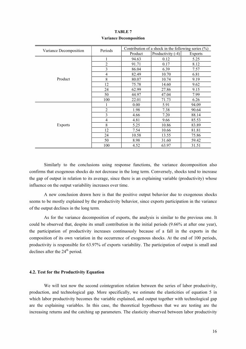
TABLE 7 Variance Decomposition

Contribution of a shock in the following series (%) Variance Decomposition Periods

Product Productivity (-4) Exports 1 94.63 0.12 5.25 2 91.71 0.17 8.12 3 86.04 6.39 7.57 4 82.49 10.70 6.81 8 80.07 10.74 9.19

12 75.78 14.60 9.62 24 62.99 27.86 9.15 50 44.97 47.04 7.99

Product

100 22.01 71.73 6.26 1 0.00 5.91 94.09 2 1.98 7.38 90.64 3 4.66 7.20 88.14 4 4.81 9.66 85.53 8 5.25 10.86 83.89

12 7.54 10.66 81.81 24 10.58 13.55 75.86 50 8.98 31.60 59.42

Exports

100 4.52 63.97 31.51 Similarly to the conclusions using response functions, the variance decomposition also

confirms that exogenous shocks do not decrease in the long term. Conversely, shocks tend to increase the gap of output in relation to its average, since there is an explaining variable (productivity) whose influence on the output variability increases over time.

A new conclusion drawn here is that the positive output behavior due to exogenous shocks seems to be mostly explained by the productivity behavior, since exports participation in the variance of the output declines in the long term.

As for the variance decomposition of exports, the analysis is similar to the previous one. It could be observed that, despite its small contribution in the initial periods (9.66% at after one year), the participation of productivity increases continuously because of a fall in the exports in the composition of its own variation in the occurrence of exogenous shocks. At the end of 100 periods, productivity is responsible for 63.97% of exports variability. The participation of output is small and declines after the 24th period. 4.2. Test for the Productivity Equation

We will test now the second cointegration relation between the series of labor productivity,

production, and technological gap. More specifically, we estimate the elasticities of equation 5 in which labor productivity becomes the variable explained, and output together with technological gap are the explaining variables. In this case, the theoretical hypotheses that we are testing are the increasing returns and the catching up parameters. The elasticity observed between labor productivity

16

and output characterizes the “Verdoorn’s Coefficient” (Thirlwall, 1987) and estimates the existence of increasing returns to scale during the period considered in the samples. On the other hand, the elasticity between technological gap and productivity estimates the effect of the technological gap between Brazil and the US. As tables 1 and 2 have already confirmed that the series considered are stationary at the 1st difference. We will perform Johansen’s test to identify the cointegration relation and cointegrating vectors (elasticities). Table 8 shows the results of this cointegration test.

TABLE 8 Johansen’s cointegration test and the number of cointegrating equations

Productivity, Output, Technological Gap

Likelihood Ratio Critical Value 5% significance

Critical value 1% Significance

Hypothesis (H0) – Number of Cointegrating

Equations 49.04799 29.68 35.65 Zero 11.76879 15.41 20.04 1 at most 2.9927 3.76 6.65 2 at most

The test equation shows an intercept at CE, an intercept at VAR, and two successive differences for the variables.

The likelihood ratio estimated is higher than the critical values at 5% and 1% of significance

which implies that the null hypothesis must be rejected, i. e., there is a cointegration relation between the series. The remaining tests indicate that there is only one statistically significant cointegrating test.

Johansen’s test also provides cointegrating parameters and their respective statistical significance described in table 9.

TABLE 9 Cointegrating Coefficients for the relation between Productivity,

Output, and Technological Gap

Productivity Output Gap Intercept 0.427826 0.68863 0.083354

Normalized Coint. Coeff. 1 1.609605 0.19483 8.827786

Statistics t (-5.03277) (-4.20572)

The second line of the table shows the normalized coefficients with the productivity

coefficient as a parameter, since in this series it is the explained variable of the last equation in the theoretical model. The output elasticity is positive, the value of which is 1.60. This means that one unit output variation causes a variation of 1.6 in unit productivity. As seen before, the fact that this coefficient is higher than 1 suggests that empirical evidence confirms the existence of increasing returns to scale in the Brazilian industry during the sampling period. Additionally, this coefficient is statistically significant at 10%.

17

The technological gap elasticity – constituting a proxy to the “absorption of new technologies” – is also positive and statistically significant at 10%. However, its magnitude is low, suggesting that one unit variation in technological gap causes a variation of 0.19 in unit productivity. Such magnitude provides the evidence that the ‘technological gap” between Brazil and US do not constitute a considerable advantage to Brazil. In other words, the technological gap did per se not bring a sufficient condition for Brazil to catch up in the period. This indicates that structural characteristics of the Brazilian national innovation system might not be contributing to an efficient absorption of the “update technology” developed in the leading country.

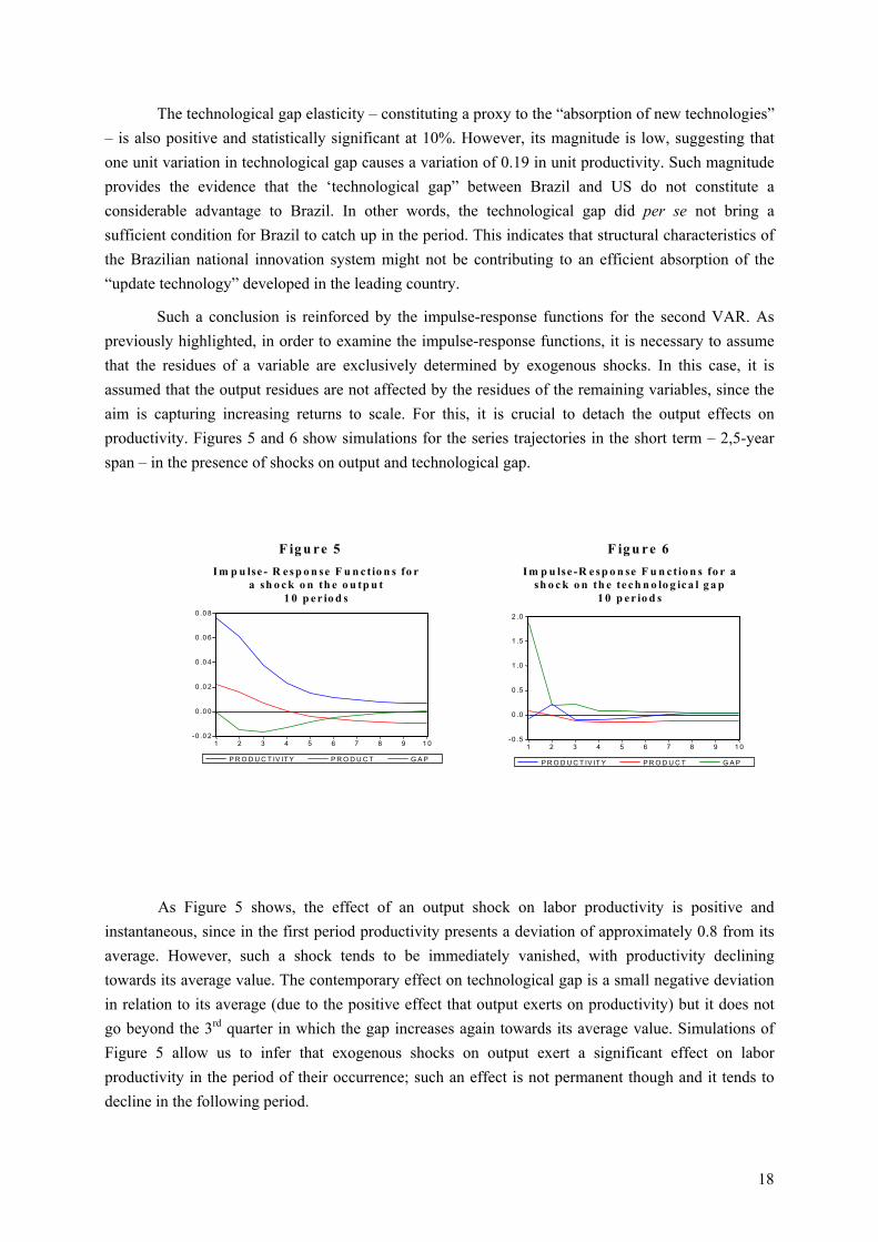
Such a conclusion is reinforced by the impulse-response functions for the second VAR. As previously highlighted, in order to examine the impulse-response functions, it is necessary to assume that the residues of a variable are exclusively determined by exogenous shocks. In this case, it is assumed that the output residues are not affected by the residues of the remaining variables, since the aim is capturing increasing returns to scale. For this, it is crucial to detach the output effects on productivity. Figures 5 and 6 show simulations for the series trajectories in the short term – 2,5-year span – in the presence of shocks on output and technological gap.

F ig u re 5 F ig u re 6

-0 .0 2

0 .0 0

0 .0 2

0 .0 4

0 .0 6

0 .0 8

1 2 3 4 5 6 7 8 9 1 0 P R O D U C T IV IT Y P R O D U C T G A P

Im p u lse - R e sp o n se F u n c tio n s fo r a sh o c k o n th e o u tp u t

1 0 p e r io d s

-0 .5

0 .0

0 .5

1 .0

1 .5

2 .0

1 2 3 4 5 6 7 8 9 1 0 P R O D U C T IV IT Y P R O D U C T G A P

Im p u lse -R e sp o n se F u n c tio n s fo r a sh o c k o n th e te c h n o lo g ic a l g a p

1 0 p e r io d s

As Figure 5 shows, the effect of an output shock on labor productivity is positive and

instantaneous, since in the first period productivity presents a deviation of approximately 0.8 from its average. However, such a shock tends to be immediately vanished, with productivity declining towards its average value. The contemporary effect on technological gap is a small negative deviation in relation to its average (due to the positive effect that output exerts on productivity) but it does not go beyond the 3rd quarter in which the gap increases again towards its average value. Simulations of Figure 5 allow us to infer that exogenous shocks on output exert a significant effect on labor productivity in the period of their occurrence; such an effect is not permanent though and it tends to decline in the following period.

18

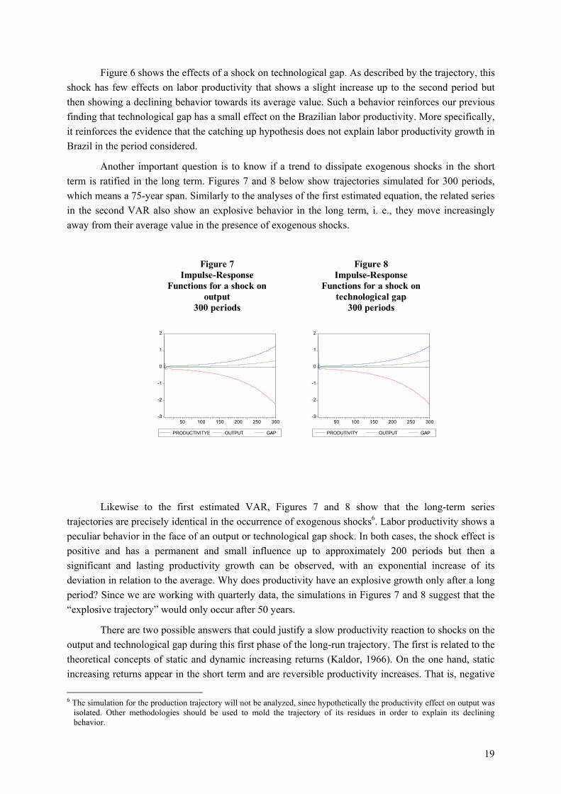
Figure 6 shows the effects of a shock on technological gap. As described by the trajectory, this shock has few effects on labor productivity that shows a slight increase up to the second period but then showing a declining behavior towards its average value. Such a behavior reinforces our previous finding that technological gap has a small effect on the Brazilian labor productivity. More specifically, it reinforces the evidence that the catching up hypothesis does not explain labor productivity growth in Brazil in the period considered.

Another important question is to know if a trend to dissipate exogenous shocks in the short term is ratified in the long term. Figures 7 and 8 below show trajectories simulated for 300 periods, which means a 75-year span. Similarly to the analyses of the first estimated equation, the related series in the second VAR also show an explosive behavior in the long term, i. e., they move increasingly away from their average value in the presence of exogenous shocks.

-3

-2

-1

0

1

2

50 100 150 200 250 300 PRODUCTIVITYE OUTPUT GAP

Figure 7 Impulse-Response

Functions for a shock on output

300 periods

-3

-2

-1

0

1

2

50 100 150 200 250 300 PRODUTIVITY OUTPUT GAP

Figure 8 Impulse-Response

Functions for a shock on technological gap

300 periods

Likewise to the first estimated VAR, Figures 7 and 8 show that the long-term series

trajectories are precisely identical in the occurrence of exogenous shocks6. Labor productivity shows a peculiar behavior in the face of an output or technological gap shock. In both cases, the shock effect is positive and has a permanent and small influence up to approximately 200 periods but then a significant and lasting productivity growth can be observed, with an exponential increase of its deviation in relation to the average. Why does productivity have an explosive growth only after a long period? Since we are working with quarterly data, the simulations in Figures 7 and 8 suggest that the “explosive trajectory” would only occur after 50 years.

There are two possible answers that could justify a slow productivity reaction to shocks on the output and technological gap during this first phase of the long-run trajectory. The first is related to the theoretical concepts of static and dynamic increasing returns (Kaldor, 1966). On the one hand, static increasing returns appear in the short term and are reversible productivity increases. That is, negative

6 The simulation for the production trajectory will not be analyzed, since hypothetically the productivity effect on output was

isolated. Other methodologies should be used to mold the trajectory of its residues in order to explain its declining behavior.

19

shocks on output will reduce gains in productivity originally obtained. On the other hand, dynamic increasing returns do not come about in the short term but they are continuous and permanent productivity increases. They stem from a longer learning period of an absorbed technology by means of labor force experiences alongside an increase of the production scale. In this way, besides providing permanent increases in productivity, the learning-by-doing process is intensified with an increase in the production scale, since the worker’s handling of a given technology is also intensified, thus allowing the labor force to proceed in a “function of technological learning”.

By looking at the impulse-response functions under an exogenous shock on output, it can be observed that the long period after which productivity starts to grow in a sustained way may be understood as the starting point of dynamic increasing returns. However, such a long period before the start of dynamic increasing returns may be an indication of difficulties the Brazilian labor force is facing to proceed in the “learning function”. Such difficulties are associated with low qualification whose proxy in the theoretical model is the average schooling of the labor force. The value of such a proxy for Brazil is actually small, since the Brazilian labor force average schooling in the sampling period is 3.7-years. Thus, one of the causes for the explosive behavior of the Brazilian productivity after so long a period is the low qualification of the labor force which hampers learning by doing along the import-substitution industrialization process. Hence, its lows down the emergence of dynamic increasing returns following an exogenous shock on output.

Another possible explanation for productivity behavior is related to the catching up hypothesis. Accordingly, the technological gap would be able to lever the growth rate of labor productivity in a backward country if this country could effectively incorporate advanced technologies being developed in the leading country. The analysis of Figure 8 shows that - after an exogenous shock on technological gap - productivity is held with a slight deviation from its average up to the period 200 showing an exponential growth afterwards. A possible interpretation for this is that the possibility of incorporation of new technologies was held constant all through the period. However, only after 50 years, the effect of technological gap would lead to the result predicted by the catching up models. That is, efficient technological absorption would be achieved and in this way pushing the Brazilian labor productivity. In other words, the benefit of a positive shock on the “technological gap” would occur only after 75 years. This would also be an indication that the Brazilian national innovation system underlining industrialization has not possessed the structural characteristics needed to incorporate the latest technologies, at least during this first phase of the long-run trajectory. As long as productivity faces an exponential growth, technological gap still shows the same growth pace, meaning that the positive reaction in productivity after 200 periods is not enough to reduce the gap, i. e., it is not enough to catch up. Such a feature reflects the low capacity of the Brazilian economy in absorbing the latest technologies that, in Abramovitz’s words (1986), is due to the low “social capability” of this economy.

Again, the variance decomposition of the forecast error for the analysis of the VAR behavior estimated in the face of exogenous shocks. As previously seen, we simulate that an arrangement of the variables is needed for the analysis. Like the arrangement of response functions, we assume that the output residues can only be explained by the behavior of the sequence εyt. Table 10 shows the contributions of each variable in explaining the residue variance behavior.

20

TABLE 10 Variance Decomposition for innovations on Productivity, Output and Gap

Contribution of an innovation in the

following series (%) Breakdown of series variance Periods Productivity Output Gap

1 7.87 92.10 0.03 2 14.43 83.28 2.29 3 22.55 74.28 3.17 4 30.70 66.16 3.14 8 53.80 44.18 2.02

12 65.75 32.64 1.61 24 80.44 18.34 1.22 50 89.10 9.91 1.00

Productivity

100 92.86 6.24 0.90 1 0 0.05 99.95 2 0.21 1.28 98.51 3 0.51 1.68 97.81 4 0.92 2.10 96.98 8 2.55 2.45 95.00

12 3.99 2.44 93.57 24 8.56 2.55 88.89 50 20.71 2.89 76.40

Gap

100 49.16 3.68 47.16 The output contribution in explaining the variance of productivity residues in the face of

innovation is extremely significant in the first 4 periods. However, a swift decline of the output contribution could also be observed, since it reached 92.10% in the first period and lowered to 44.18% at the end of the 8th period. Conversely, the participation of productivity rises rapidly in explaining its own variance, reaching 53.8% in the 8th quarter. This confirms the fact observed by the analysis of response functions: the existence of increasing returns to scale is not sufficient to perpetuate positive impacts on productivity in the presence of exogenous shocks on output and the reason for this is possibly the characteristics of the learning function. Additionally, the participation of technological gap in explaining the productivity variability (3.17% at most in the 3rd period) is too small, which confirms the conclusion that the relevance of technological gap for the Brazilian labor productivity growth via “technological imitation” is negligible. 5. CONCLUSIONS

The tests performed in this paper revealed a cointegration relation between the variables

studied. The first long-term relation (output, productivity, and exports) presented statistically significant coefficients with the signal predicted by the theory, i. e., productivity and exports relate positively to the output behavior. In the case of productivity, this was only obtained when lagged series was considered in 4 periods, showing that the effects of labor productivity variation can only exert significant impacts on the output after an one-year span.

21

Another interesting finding is that the hypothesis of “growth led by exports” was only partially confirmed for Brazil during the sampling period considered. This may evidence that exports were not the major component of the Brazilian demand during the period. In accordance to Kaldor (1966), this suggests that demand pulled by “domestic market” is not exhausted yet while exports might play an import but complementary role. And Myrdal/Kaldor cumulative causality could be verified by means of a model of error correction. On the other hand, Jayme Jr (2003) shows that, in the period of 1955-2000, Brazilian output growth has been constrained by balance of payments that is not made endogenous in our model. Bértola, Higachi, and Porcile (2002) have also showed the relevance of external constraints in the country’s economic growth.

We think that a remarkable finding is the cumulative effect of an exogenous productivity shocks on output and exports. Besides confirming a significant effect of productivity on output only after a one-year period, the impulse-response functions also showed that a productivity shock does not tend to dissipate over time. Conversely, it tends to move away from the series of its average values. This result indicates the need for more detailed empirical studies that could explain the “explosive behavior”.

Estimations of the theoretical equation related to productivity, output, and technological gap show interesting results. The elasticity for the increasing returns to scale is significant and relevant in magnitude. However, exogenous shocks on output have a powerful effect only on labor productivity after a one-year period, by provoking a slight deviation on productivity behavior during 200 periods. This evidences the difficulties placed for the dynamic increasing returns in the Brazilian economy, which seems to be unable accumulate gains from technological learning.

The coefficient of technological gap and labor productivity – in spite of being significant and positive – shows a relatively small magnitude. The Brazilian technological gap does not seem to represent a sufficient condition for an efficient absorption of technologies from the leading country (the USA). That is to say, Brazil is only partially able to catch up, since it cannot manage to fully engage in the international technological diffusion since it faces difficulties in absorbing the latest technologies.

The impulse-response function simulations for the long term show that – in the presence of an exogenous output or technological gap shock – productivity will only show an explosive behavior after a fifty-year period. The theory provides two possible explanations for such a trajectory.

The first is related to the dynamic increasing returns stemming from the capacity the labor force possesses with a given technology in function of an increased production scale. Such a learning-by-doing process becomes significant to the extent that output growth allows the intensification of the labor force specialization in a given technology. Using impulse-response functions, the period in which productivity increases exponentially may be understood as the starting point of the effects of dynamic increasing returns or, in other words, the instant in which the labor force starts to advance in a “technological learning function”. The key aspect is that the greater the labor force qualification, the faster the emergence of dynamic increasing returns. In this sense, the long period in which such effects become relevant (only after 50 years) may be due to the low qualification of the Brazilian labor force, which hampers increases in productivity stemming from learning by doing.

22

The second reason refers to the productivity behavior in the long term after a technological gap shock. This could also evidence the Brazilian economy constraints in absorbing the latest technologies from the leading countries. It seems that growth via technological imitation was possible all through 200 periods but only afterwards it started to increase exponentially. Such a result suggests that there are restraints on “social capability”, impeding the Brazilian economy to benefit fully from the “advantages from the gap”. This is a possible result of the characteristics of Brazilian import-substitution industrialization. The resulting national innovation system is not working as a focal tool able to provide “windows of opportunity”, being considered as “immature” (Albuquerque, 1999).

. Besides, the impulse-response functions reveal that technological gap also increase exponentially when productivity has the same growth, which suggests that technological absorption after 200 periods is not enough to reduce the gap. This is to say that the opportunities for Brazil to catch up seems to be blocked in the long term due to difficulties in absorbing technologies.

In spite of model’s restricted proxy for the capacity of technological absorption, it seems that labor-force average schooling is important enough for Brazil to increase its technological absorption potential. This is a key feature in the model, since the specification of the catching up function (aG e (-

G/δ)) requires that the limit to technological imitation will reach its peak when the gap is equal to the average schooling7. If the gap is higher, this means that the country does not possess the least conditions to absorb technology from the leading country and hence gains in productivity are increasingly smaller to the extent that the gap increases.

The evidences of increasing returns from 1976 to 2000 should not overshadow the main conclusion of this paper. It suggests the presence of structural constraints to the Brazilian economy that holds back permanent gains in labor productivity based on learning by doing. Associated to this, Brazil does not catch up efficiently, i. e.; its economy seems not to benefit fully from international technological diffusion. This again suggests structural constraints preventing Brazil to absorb technologies and hence spur its technological progress.

7 This happens because G must be equal to δ so that the derivative of function G and (-G/δ) be equal to zero.

23

REFERENCES

Abramovitz, M. (1986). Catching Up, Forging Ahead, and Falling Behind. Journal of Economic History, New York, v. 66, n. 2, p. 385-406, junho.

Albuquerque, E. (1999). National Systems of Innovation and Non-OECD Countries: Notes About a Rudimentary and Tentative “Typology”. Revista de Economia Política, vol. 19, nº 4 (76), outubro-dezembro.

Bértola, L. Higachi, H. Porcile, G. (2002). Balance-of-payments-constrained growth in Brazil: a test of Thirlwall’s Law, 1890-1973. Journal of Post Keynesian Economics, New York, v. 25, n. 1, p. 123-140, Fall.

Blitch, C. P. (1983). Allyn Young on increasing returns. Journal of Post Keynesian Economics, New York, v. 5, n. 3, p. 359-372, Spring.

Charemza, W. W. & Deadman, D. F. (1997). New Directions In Econometric Practice. London: Edward Elgar.

Dixon, R. & Thirlwall, A. P. (1975). A Model Of Regional Growth-Rate Differences On Kaldorian Lines. Oxford Economic Papers. July.

Enders, W. (1995). Applied Econometric Time Series. New York, Iowa University.

Fagerberg, J. (1988a). Why growth rates differ. In: DOSI, G. et alli. Technical Change and Economic Theory. London: Pinter.

Fagerberg, J. (1988b). International Competitiveness. The Economic Journal, 98, June, pp. 355-74

Freeman, C. (1995). The “National System of Innovation” in historical perspective. Cambridge Journal of Economics, Cambridge, v. 19, n.1, p. 5-24.

Jayme Jr, F. G. (2003). Balanced-of-Payments Constrained Economic Growth In Brazil. Revista de Economia Política, v.23, n.1, Jan/Abr.

Hamilton, J. (1994). Time Series Analysis. Princeton University Press.

Higachi, H. Canuto, O. Porcile, G. (1999). Modelos Evolucionistas de Crescimento Endógeno. Revista de Economia Política, vol. 19, nº 4 (76), outubro-dezembro.

Holden, D. & Perman, R. (1994). Unit Roots and Cointegration For The Economist. In: Rao, B. B. (org.) Cointegration For The Applied Economist. New York: Martin’s Press.

Kaldor, N. (1966). Causes Of The Slow Rate Of Economic Growth Of The United Kingdom. In: KING, J. E. Economic Growth in Theory and Practice: a Kaldorian Perspective. Cambridge: Edward Elgar, p. 279-318, 1994.

Lewis, W. A. (1969). O Desenvolvimento Econômico Com Oferta Ilimitada De Mão-De-Obra. In: AGARWALA, A. N. & SINGH, S. P. (orgs). A Economia Do Subdesenvolvimento. Rio de Janeiro: Forence, p. 406-456.

24

Madalla, G.S. & In-Moo Kim (1998). Unit Roots, Cointegration and Structural Change. Cambridge University Press, Cambridge, UK.

Mccombie, J. S. L. (1983). Kaldor’s laws in retrospect. Journal of Post Keynesian Economics, New York, v. 5, n. 3, p. 414-429, Spring.

Mccombie, J. S. L. & Thirlwall, A. P. (1994). Economic Growth and the Balance-of-Payments Constraint. New York: Martin’s Press.

Mills, T. C. (1993). The Econometric Modelling of Financial Time Series. New York: Cambridge.

Nelson, R. R. (org.) (1993). National Innovation Systems: a comparative analysis. New York, Oxford: Oxford University.

Perez, C. & Soete, L. (1988). Catching up in technology: entry barriers and windows of opportunity. In: In: DOSI, G. et al. Technical Change and Economic Theory. London: Pinter, p. 458-479.

Schumpeter, J. A. (1933). Teoria do Desenvolvimento Econômico. São Paulo: Abril Cultural, 1988.

Schumpeter, J. A. (1943). Capitalismo, Socialismo e Democracia. Rio de Janeiro: Zahar, 1984.

Thirlwall, A. P. (1987). Nicholas Kaldor. New York: N.Y. University Press.

25