Textbook Query Optimization 2. Textbook Query...
41
28 / 575 Textbook Query Optimization 2. Textbook Query Optimization • Algebra Revisited • Canonical Query Translation • Logical Query Optimization • Physical Query Optimization
Transcript of Textbook Query Optimization 2. Textbook Query...
28 / 575
Textbook Query Optimization
2. Textbook Query Optimization
• Algebra Revisited
• Canonical Query Translation
• Logical Query Optimization
• Physical Query Optimization
29 / 575
Textbook Query Optimization Algebra Revisited
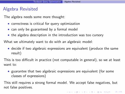
Algebra Revisited
The algebra needs some more thought:
• correctness is critical for query optimization
• can only be guaranteed by a formal model
• the algebra description in the introduction was too cursory
What we ultimately want to do with an algebraic model:
• decide if two algebraic expressions are equivalent (produce the sameresult)
This is too difficult in practice (not computable in general), so we at leastwant to:
• guarantee that two algebraic expressions are equivalent (for someclasses of expressions)
This still requires a strong formal model. We accept false negatives, butnot false positives.

30 / 575
Textbook Query Optimization Algebra Revisited
Tuples
Tuple:
• a (unordered) mapping from attribute names to values of a domain
• sample: [name: ”Sokrates”, age: 69]
Schema:
• a set of attributes with domain, written A(t)
• sample: {(name,string),(age, number)}
Note:
• simplified notation on the slides, but has to be kept in mind
• domain usually omitted when not relevant
• attribute names omitted when schema known
31 / 575
Textbook Query Optimization Algebra Revisited
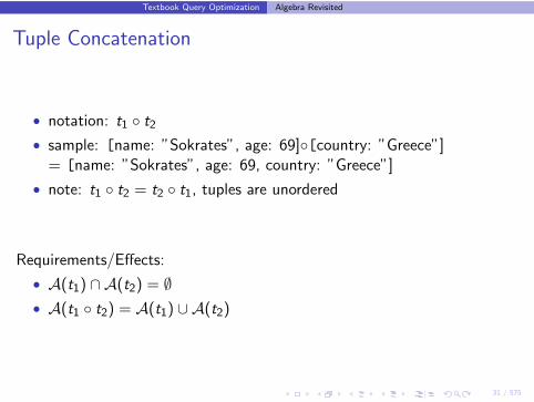
Tuple Concatenation
• notation: t1 ◦ t2
• sample: [name: ”Sokrates”, age: 69]◦[country: ”Greece”]= [name: ”Sokrates”, age: 69, country: ”Greece”]
• note: t1 ◦ t2 = t2 ◦ t1, tuples are unordered
Requirements/Effects:
• A(t1) ∩ A(t2) = ∅
• A(t1 ◦ t2) = A(t1) ∪ A(t2)
32 / 575
Textbook Query Optimization Algebra Revisited
Tuple Projection
Consider t = [name: ”Sokrates”, age: 69, country: ”Greece”]
Single Attribute:
• notation t.a
• sample: t.name = ”Sokrates”
Multiple Attributes:
• notation t|A
• sample: t|{name,age} = [name: ”Sokrates”, age: 69]
Requirements/Effects:
• a ∈ A(t), A ⊆ A(t)
• A(t|A) = A
• notice: t.a produces a value, t|A produces a tuple
33 / 575
Textbook Query Optimization Algebra Revisited
Relations
Relation:
• a set of tuples with the same schema
• sample: {[name: ”Sokrates”, age: 69], [name: ”Platon”, age: 45]}
Schema:
• schema of the contained tuples, written A(R)
• sample: {(name,string),(age, number)}
34 / 575
Textbook Query Optimization Algebra Revisited
Sets vs. Bags
• relations are sets of tuples
• real data is usually a multi set (bag)
Example: select agefrom student
age
232424. . .
• we concentrate on sets first for simplicity
• many (but not all) set equivalences valid for bags
The optimizer must consider three different semantics:
• logical algebra operates on bags
• physical algebra operates on streams (order matters)
• explicit duplicate elimination ⇒ sets
35 / 575
Textbook Query Optimization Algebra Revisited
Set Operations
Set operations are part of the algebra:
• union (L ∪ R), intersection (L ∩ R), difference (L \ R)
• normal set semantic
• but: schema constraints
• for bags defined via frequencies (union → +, intersection → min,difference → −)
Requirements/Effects:
• A(L) = A(R)
• A(L ∪ R) = A(L) = A(R), A(L ∩ R) = A(L) = A(R),A(L \ R) = A(L) = A(R)
36 / 575
Textbook Query Optimization Algebra Revisited
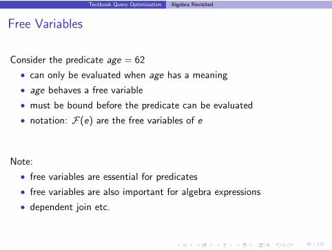
Free Variables
Consider the predicate age = 62
• can only be evaluated when age has a meaning
• age behaves a free variable
• must be bound before the predicate can be evaluated
• notation: F(e) are the free variables of e
Note:
• free variables are essential for predicates
• free variables are also important for algebra expressions
• dependent join etc.
37 / 575
Textbook Query Optimization Algebra Revisited
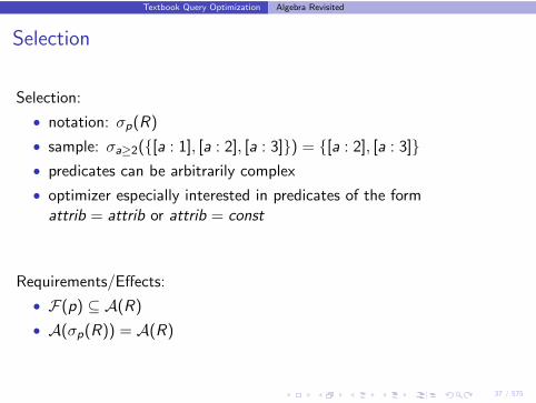
Selection
Selection:
• notation: σp(R)
• sample: σa≥2({[a : 1], [a : 2], [a : 3]}) = {[a : 2], [a : 3]}
• predicates can be arbitrarily complex
• optimizer especially interested in predicates of the formattrib = attrib or attrib = const
Requirements/Effects:
• F(p) ⊆ A(R)
• A(σp(R)) = A(R)
38 / 575
Textbook Query Optimization Algebra Revisited
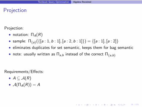
Projection
Projection:
• notation: ΠA(R)
• sample: Π{a}({[a : 1, b : 1], [a : 2, b : 1]}) = {[a : 1], [a : 2]}
• eliminates duplicates for set semantic, keeps them for bag semantic
• note: usually written as Πa,b instead of the correct Π{a,b}
Requirements/Effects:
• A ⊆ A(R)
• A(ΠA(R)) = A
39 / 575
Textbook Query Optimization Algebra Revisited
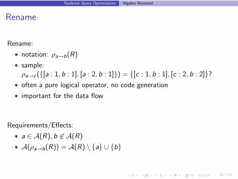
Rename
Rename:
• notation: ρa→b(R)
• sample:ρa→c({[a : 1, b : 1], [a : 2, b : 1]}) = {[c : 1, b : 1], [c : 2, b : 2]}?
• often a pure logical operator, no code generation
• important for the data flow
Requirements/Effects:
• a ∈ A(R), b 6∈ A(R)
• A(ρa→b(R)) = A(R) \ {a} ∪ {b}
40 / 575
Textbook Query Optimization Algebra Revisited
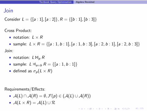
Join
Consider L = {[a : 1], [a : 2]},R = {[b : 1], [b : 3]}
Cross Product:
• notation: L× R
• sample: L× R = {[a : 1, b : 1], [a : 1, b : 3], [a : 2, b : 1], [a : 2, b : 3]}
Join:
• notation: L �p R
• sample: L �a=b R = {[a : 1, b : 1]}
• defined as σp(L× R)
Requirements/Effects:
• A(L) ∩ A(R) = ∅,F(p) ∈ (A(L) ∪ A(R))
• A(L× R) = A(L) ∪R
41 / 575
Textbook Query Optimization Algebra Revisited
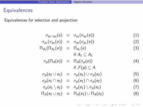
Equivalences
Equivalences for selection and projection:
σp1∧p2(e) ≡ σp1(σp2(e)) (1)
σp1(σp2(e)) ≡ σp2(σp1(e)) (2)
ΠA1(ΠA2(e)) ≡ ΠA1(e) (3)
if A1 ⊆ A2
σp(ΠA(e)) ≡ ΠA(σp(e)) (4)
if F(p) ⊆ A
σp(e1 ∪ e2) ≡ σp(e1) ∪ σp(e2) (5)
σp(e1 ∩ e2) ≡ σp(e1) ∩ σp(e2) (6)
σp(e1 \ e2) ≡ σp(e1) \ σp(e2) (7)
ΠA(e1 ∪ e2) ≡ ΠA(e1) ∪ ΠA(e2) (8)
42 / 575
Textbook Query Optimization Algebra Revisited
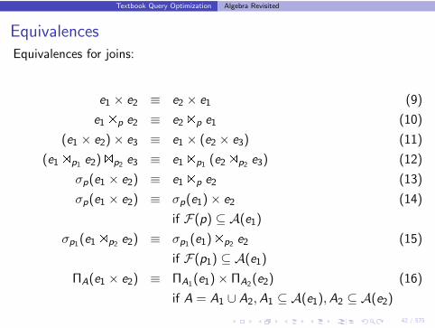
Equivalences
Equivalences for joins:
e1 × e2 ≡ e2 × e1 (9)
e1 �p e2 ≡ e2 �p e1 (10)
(e1 × e2)× e3 ≡ e1 × (e2 × e3) (11)
(e1 �p1 e2) �p2 e3 ≡ e1 �p1 (e2 �p2 e3) (12)
σp(e1 × e2) ≡ e1 �p e2 (13)
σp(e1 × e2) ≡ σp(e1)× e2 (14)
if F(p) ⊆ A(e1)
σp1(e1 �p2 e2) ≡ σp1(e1) �p2 e2 (15)
if F(p1) ⊆ A(e1)
ΠA(e1 × e2) ≡ ΠA1(e1)× ΠA2(e2) (16)
if A = A1 ∪ A2, A1 ⊆ A(e1), A2 ⊆ A(e2)
43 / 575
Textbook Query Optimization Canonical Query Translation
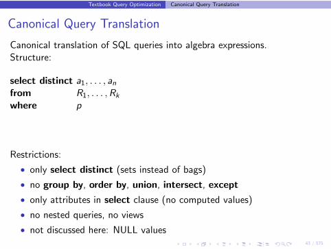
Canonical Query Translation
Canonical translation of SQL queries into algebra expressions.Structure:
select distinct a1, . . . , an
from R1, . . . ,Rk
where p
Restrictions:
• only select distinct (sets instead of bags)
• no group by, order by, union, intersect, except
• only attributes in select clause (no computed values)
• no nested queries, no views
• not discussed here: NULL values
44 / 575
Textbook Query Optimization Canonical Query Translation
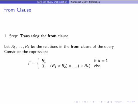
From Clause
1. Step: Translating the from clause
Let R1, . . . ,Rk be the relations in the from clause of the query.Construct the expression:
F =
{
R1 if k = 1((. . . (R1 × R2)× . . .)× Rk) else
45 / 575
Textbook Query Optimization Canonical Query Translation
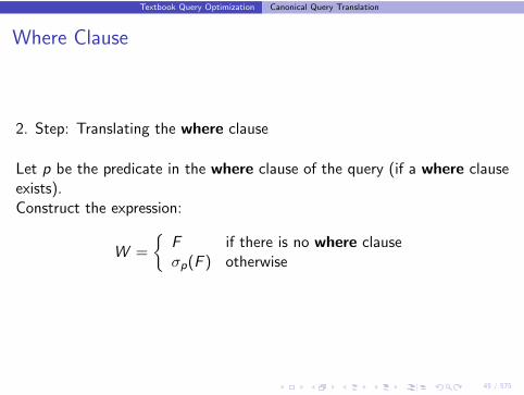
Where Clause
2. Step: Translating the where clause
Let p be the predicate in the where clause of the query (if a where clauseexists).Construct the expression:
W =
{
F if there is no where clauseσp(F ) otherwise
46 / 575
Textbook Query Optimization Canonical Query Translation
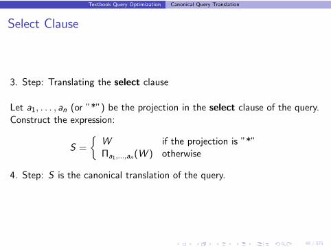
Select Clause
3. Step: Translating the select clause
Let a1, . . . , an (or ”*”) be the projection in the select clause of the query.Construct the expression:
S =
{
W if the projection is ”*”Πa1,...,an(W ) otherwise
4. Step: S is the canonical translation of the query.
47 / 575
Textbook Query Optimization Canonical Query Translation
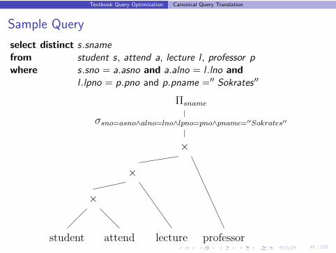
Sample Query
select distinct s.sname
from student s, attend a, lecture l , professor p
where s.sno = a.asno and a.alno = l .lno and
l .lpno = p.pno and p.pname =′′ Sokrates ′′
Πsname
σsno=asno∧alno=lno∧lpno=pno∧pname=′′Sokrates′′
×
×
×
professorlectureattendstudent
48 / 575
Textbook Query Optimization Canonical Query Translation
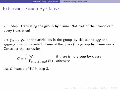
Extension - Group By Clause
2.5. Step: Translating the group by clause. Not part of the ”canonical”query translation!
Let g1, . . . , gm be the attributes in the group by clause and agg theaggregations in the select clause of the query (if a group by clause exists).Construct the expression:
G =
{
W if there is no group by clauseΓg1,...,gm;agg (W ) otherwise
use G instead of W in step 3.
49 / 575
Textbook Query Optimization Logical Query Optimization
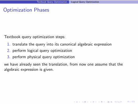
Optimization Phases
Textbook query optimization steps:
1. translate the query into its canonical algebraic expression
2. perform logical query optimization
3. perform physical query optimization
we have already seen the translation, from now one assume that thealgebraic expression is given.
50 / 575
Textbook Query Optimization Logical Query Optimization
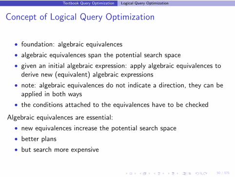
Concept of Logical Query Optimization
• foundation: algebraic equivalences
• algebraic equivalences span the potential search space
• given an initial algebraic expression: apply algebraic equivalences toderive new (equivalent) algebraic expressions
• note: algebraic equivalences do not indicate a direction, they can beapplied in both ways
• the conditions attached to the equivalences have to be checked
Algebraic equivalences are essential:
• new equivalences increase the potential search space
• better plans
• but search more expensive
51 / 575
Textbook Query Optimization Logical Query Optimization
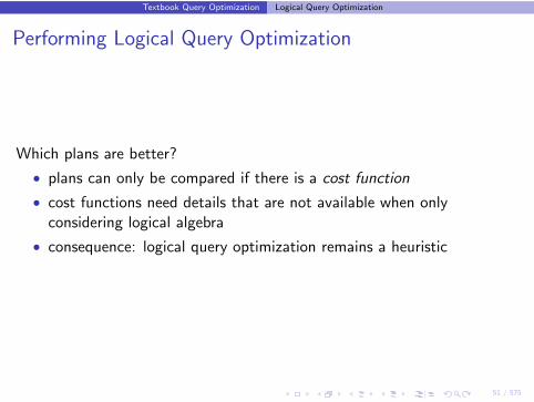
Performing Logical Query Optimization
Which plans are better?
• plans can only be compared if there is a cost function
• cost functions need details that are not available when onlyconsidering logical algebra
• consequence: logical query optimization remains a heuristic
52 / 575
Textbook Query Optimization Logical Query Optimization
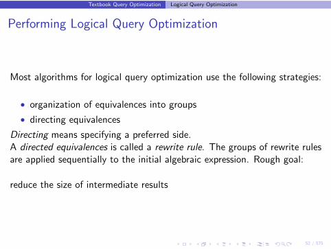
Performing Logical Query Optimization
Most algorithms for logical query optimization use the following strategies:
• organization of equivalences into groups
• directing equivalences
Directing means specifying a preferred side.A directed equivalences is called a rewrite rule. The groups of rewrite rulesare applied sequentially to the initial algebraic expression. Rough goal:
reduce the size of intermediate results
53 / 575
Textbook Query Optimization Logical Query Optimization
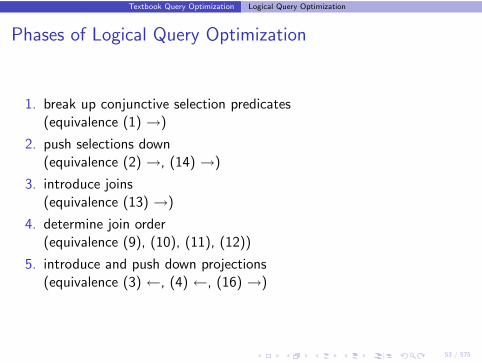
Phases of Logical Query Optimization
1. break up conjunctive selection predicates(equivalence (1) →)
2. push selections down(equivalence (2) →, (14) →)
3. introduce joins(equivalence (13) →)
4. determine join order(equivalence (9), (10), (11), (12))
5. introduce and push down projections(equivalence (3) ←, (4) ←, (16) →)
54 / 575
Textbook Query Optimization Logical Query Optimization
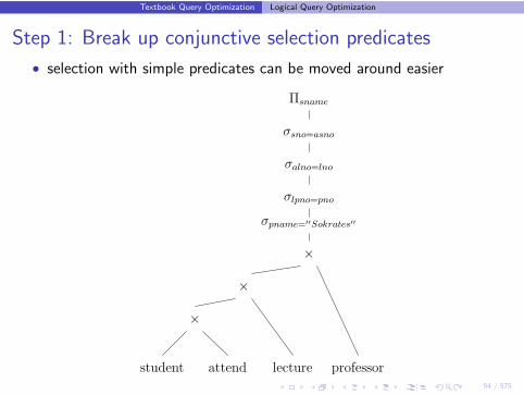
Step 1: Break up conjunctive selection predicates
• selection with simple predicates can be moved around easier
σpname=′′Sokrates′′
σsno=asno
σalno=lno
σlpno=pno
student attend lecture professor
×
×
×
Πsname
55 / 575
Textbook Query Optimization Logical Query Optimization
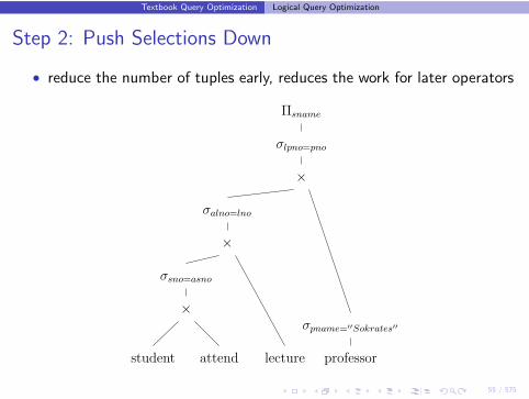
Step 2: Push Selections Down
• reduce the number of tuples early, reduces the work for later operators
σpname=′′Sokrates′′
σsno=asno
σalno=lno
σlpno=pno
student attend lecture professor
×
×
×
Πsname
56 / 575
Textbook Query Optimization Logical Query Optimization
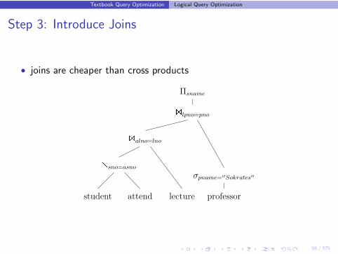
Step 3: Introduce Joins
• joins are cheaper than cross products�lpno=pno�alno=lno�sno=asno
σpname=′′Sokrates′′
student attend lecture professor
Πsname
57 / 575
Textbook Query Optimization Logical Query Optimization
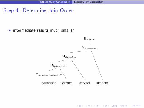
Step 4: Determine Join Order
• costs differ vastly
• difficult problem, NP hard (next chapter discusses only join ordering)
Observations in the sample plan:
• bottom most expression isstudent �sno=asno attend
• the result is huge, all students, all their lectures
• in the result only one professor relevantσname=′′Sokrates′′(professor)
• join this with lecture first, only lectures by him, much smaller
58 / 575
Textbook Query Optimization Logical Query Optimization
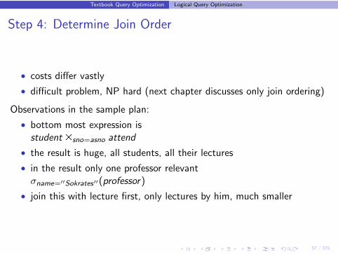
Step 4: Determine Join Order
• intermediate results much smaller
�lpno=pno
�alno=lno
�sno=asno
σpname=′′Sokrates′′
studentattendlectureprofessor
Πsname
59 / 575
Textbook Query Optimization Logical Query Optimization
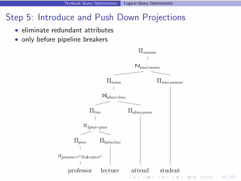
Step 5: Introduce and Push Down Projections
• eliminate redundant attributes• only before pipeline breakers
Πlpno,lno
Πsname
professor lecture attend student
σpname=′′Sokrates′′
�sno=asno�alno=lno�lpno=pno
Πpno
Πlno Πalno,asno
Πasno Πsno,sname
60 / 575
Textbook Query Optimization Logical Query Optimization
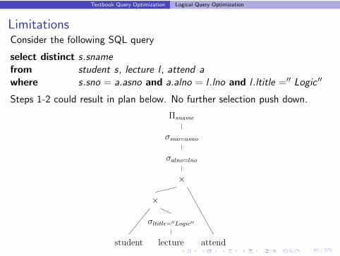
LimitationsConsider the following SQL query
select distinct s.sname
from student s, lecture l , attend a
where s.sno = a.asno and a.alno = l .lno and l .ltitle =′′ Logic ′′
Steps 1-2 could result in plan below. No further selection push down.
σalno=lno
σsno=asno
student attendlecture
×
×
Πsname
σltitle=′′Logic′′
61 / 575
Textbook Query Optimization Logical Query Optimization
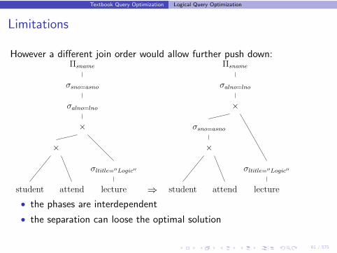
Limitations
However a different join order would allow further push down:
σalno=lno
σsno=asno
student attend lecture
×
×
Πsname
σltitle=′′Logic′′
⇒
σalno=lno
σsno=asno
student attend lecture
×
×
Πsname
σltitle=′′Logic′′
• the phases are interdependent
• the separation can loose the optimal solution

62 / 575
Textbook Query Optimization Physical Query Optimization
Physical Query Optimization
• add more execution information to the plan
• allow for cost calculations
• select index structures/access paths
• choose operator implementations
• add property enforcer
• choose when to materialize (temp/DAGs)
63 / 575
Textbook Query Optimization Physical Query Optimization
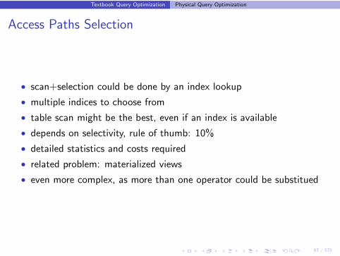
Access Paths Selection
• scan+selection could be done by an index lookup
• multiple indices to choose from
• table scan might be the best, even if an index is available
• depends on selectivity, rule of thumb: 10%
• detailed statistics and costs required
• related problem: materialized views
• even more complex, as more than one operator could be substitued
64 / 575
Textbook Query Optimization Physical Query Optimization
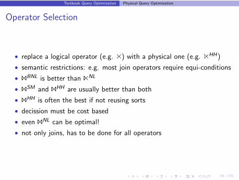
Operator Selection
• replace a logical operator (e.g. �) with a physical one (e.g. �HH)
• semantic restrictions: e.g. most join operators require equi-conditions
• �BNL is better than �NL
• �SM and �HH are usually better than both
• �HH is often the best if not reusing sorts
• decission must be cost based
• even �NL can be optimal!
• not only joins, has to be done for all operators
65 / 575
Textbook Query Optimization Physical Query Optimization
Property Enforcer
• certain physical operators need certain properties
• typical example: sort for �SM
• other example: in a distributed database operators need the datalocally to operate
• many operator requirements can be modeled as properties (hashingetc.)
• have to be guaranteed as needed
66 / 575
Textbook Query Optimization Physical Query Optimization
Materializing
• sometimes materializing is a good idea
• temp operator stores input on disk
• essential for multiple consumers (factorization, DAGs)
• also relevant for �NL
• first pass expensive, further passes cheap
67 / 575
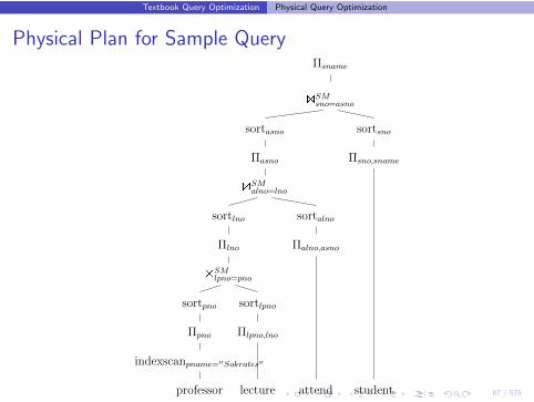
Textbook Query Optimization Physical Query Optimization
Physical Plan for Sample Query �SMsno=asno
�SMalno=lno
sortsno
sortalno
sortasno
indexscanpname=′′Sokrates′′
sortlno�SMlpno=pno
sortlpnosortpno
Πsno,snameΠasno
Πalno,asnoΠlno
Πpno
studentattendlectureprofessor
Πsname
Πlpno,lno
68 / 575
Textbook Query Optimization Physical Query Optimization
Outlook
• separation in two phases looses optimality
• many decissions (e.g. view resolution) important for logicaloptimization
• textbook physical optimization is incomplete
• did not discuss cost calculations
• will look at this again in later chapters