TEXT MINING FOR SOCIAL HARM AND CRIMINAL JUSTICE

APPLICATIONS

A Thesis

Submitted to the Faculty

of

Purdue University

by

Ritika Pandey

In Partial Fulfillment of the

Requirements for the Degree

of

Master of Science

August 2020

Purdue University

Indianapolis, Indiana

ii

THE PURDUE UNIVERSITY GRADUATE SCHOOL

STATEMENT OF THESIS APPROVAL

Dr. George Mohler, Chair

Department of Computer and Information Science

Dr. Mohammad Al Hasan

Department of Computer and Information Science

Dr. Snehasis Mukhopadhyay

Department of Computer and Information Science

Approved by:

Dr. Mihran Tuceryan

Head of Graduate Program

iii

To my parents.

iv

ACKNOWLEDGMENTS

I would like to express my sincere thanks to my advisor, Dr. George Mohler, for

his continuous guidance, encouragement and mentorship throughout my studies and

this research. I am gratefully indebted to him for his patience and support. I could

not have imagined having a better advisor and mentor.

I am extremely grateful to Professor Mohammad Al Hasan and Professor Snehasis

Mukopadhyay, for their guidance in completing this work.

My sincere thanks goes to John and Sumati for all their excellent work in Addiction

project. I would also like to thank Dr. P. Jeffrey Brantingham for his help and advice

in homicide project.

To conclude, I cannot forget to thank my family and friends for all the uncondi-

tional support and encouragement.

v

TABLE OF CONTENTS

Page

LIST OF TABLES . . . . . . . . . . . . . . . . . . . . . . . . . . . . . . . . . . vii

LIST OF FIGURES . . . . . . . . . . . . . . . . . . . . . . . . . . . . . . . . . viii

ABSTRACT . . . . . . . . . . . . . . . . . . . . . . . . . . . . . . . . . . . . . x

1 INTRODUCTION . . . . . . . . . . . . . . . . . . . . . . . . . . . . . . . . 1

1.1 Thesis Outline . . . . . . . . . . . . . . . . . . . . . . . . . . . . . . . . 3

2 EVALUATION OF CRIME TOPIC MODELS: TOPIC COHERENCE VER-

SUS SPATIAL CRIME CONCENTRATION . . . . . . . . . . . . . . . . . . 4

2.1 Introduction . . . . . . . . . . . . . . . . . . . . . . . . . . . . . . . . . 4

2.2 Methods . . . . . . . . . . . . . . . . . . . . . . . . . . . . . . . . . . . 6

2.3 Results . . . . . . . . . . . . . . . . . . . . . . . . . . . . . . . . . . . . 8

2.4 Conclusion . . . . . . . . . . . . . . . . . . . . . . . . . . . . . . . . . . 10

3 REDDITORS IN RECOVERY: TEXT MINING REDDIT TO INVESTI-

GATE TRANSITIONS INTO DRUG ADDICTION . . . . . . . . . . . . . . 12

3.1 Introduction . . . . . . . . . . . . . . . . . . . . . . . . . . . . . . . . . 12

3.2 Background and Related Works . . . . . . . . . . . . . . . . . . . . . . 13

3.2.1 Drug Addiction and the Opioid Crisis . . . . . . . . . . . . . . . 13

3.2.2 Using Social Media to Understand Drug-Related Issues . . . . . 15

3.3 Reddit Data . . . . . . . . . . . . . . . . . . . . . . . . . . . . . . . . . 16

3.4 Transition Classification: Modelling Transitions from Recreational Use

to Substance Abuse . . . . . . . . . . . . . . . . . . . . . . . . . . . . . 17

3.4.1 Creating Classes . . . . . . . . . . . . . . . . . . . . . . . . . . 17

3.4.2 Feature Selection . . . . . . . . . . . . . . . . . . . . . . . . . . 18

3.5 Survival Analysis: Predicting When Transitions are Likely to Occur . . 22

3.5.1 Right-Censored Data . . . . . . . . . . . . . . . . . . . . . . . . 23

3.5.2 Cox Regression . . . . . . . . . . . . . . . . . . . . . . . . . . . 23

vi

Page

3.6 Results . . . . . . . . . . . . . . . . . . . . . . . . . . . . . . . . . . . . 24

3.6.1 Survival Predictions on the Transition Dataset . . . . . . . . . . 26

3.7 Case Study . . . . . . . . . . . . . . . . . . . . . . . . . . . . . . . . . 27

3.7.1 Model Predictions of Subject . . . . . . . . . . . . . . . . . . . 28

3.8 Discussion . . . . . . . . . . . . . . . . . . . . . . . . . . . . . . . . . . 28

3.8.1 Informing Culture and Classifications . . . . . . . . . . . . . . . 30

3.8.2 Limitations . . . . . . . . . . . . . . . . . . . . . . . . . . . . . 31

3.9 Future Work . . . . . . . . . . . . . . . . . . . . . . . . . . . . . . . . . 32

4 BUILDING KNOWLEDGE GRAPHS OF HOMICIDE INVESTIGATION

CHRONOLOGIES . . . . . . . . . . . . . . . . . . . . . . . . . . . . . . . . 33

4.1 Introduction . . . . . . . . . . . . . . . . . . . . . . . . . . . . . . . . . 33

4.2 Homicide Graph Ontologies . . . . . . . . . . . . . . . . . . . . . . . . 35

4.3 Data Description . . . . . . . . . . . . . . . . . . . . . . . . . . . . . . 36

4.4 Identifying Named Entities and Evidence . . . . . . . . . . . . . . . . . 37

4.4.1 SpaCy . . . . . . . . . . . . . . . . . . . . . . . . . . . . . . . . 37

4.4.2 Bidirectional LSTM-CRF . . . . . . . . . . . . . . . . . . . . . 39

4.4.3 Application of NER to homicide investigation chronologies . . . 40

4.4.4 Identifying Evidence using Keyword Expansion . . . . . . . . . 40

4.5 Building a Knowledge Graph of Homicide Investigation Chronologies . 42

4.6 Association between Knowledge Graph Features and Homicide Solvability44

4.7 Discussion . . . . . . . . . . . . . . . . . . . . . . . . . . . . . . . . . . 49

5 SUMMARY . . . . . . . . . . . . . . . . . . . . . . . . . . . . . . . . . . . . 52

6 PUBLICATIONS . . . . . . . . . . . . . . . . . . . . . . . . . . . . . . . . . 54

REFERENCES . . . . . . . . . . . . . . . . . . . . . . . . . . . . . . . . . . . . 55

vii

LIST OF TABLES

Table Page

2.1 Coherence vs. spatial concentration 2009-2014 . . . . . . . . . . . . . . . . 9

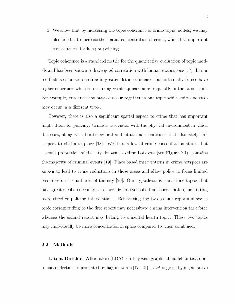
2.2 Category 2014 . . . . . . . . . . . . . . . . . . . . . . . . . . . . . . . . . . 10

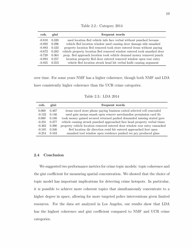
2.3 LDA 2014 . . . . . . . . . . . . . . . . . . . . . . . . . . . . . . . . . . . . 10

3.1 Discriminatory keywords for CAS and CAS→RECOV class using OddsRatio . . . . . . . . . . . . . . . . . . . . . . . . . . . . . . . . . . . . . . 21

3.2 Transition Classifier Results Summary. Table displays test-set performance

of Random Forest with 170 trees (selected using grid search and 10-fold cross

validation) using different features. Model trained on users’ first 6 months of

posts and predicts transitions in the subsequent 12 months. Number of train

and test set examples were 352 and 88, respectively. . . . . . . . . . . . . . . 25

3.3 Cox Model Results Summary. Train/test split of 1,775 (1665 censored) and

592 (352 censored) users, respectively. C-Index shown for models using different

feature sets. The model using drug utterances, keywords, and LIWC features

performed best on training set using 5-fold cross validation and gave a test-

set C-Index of 0.820. Test set data consisted of 45 observed and 592 censored

examples. . . . . . . . . . . . . . . . . . . . . . . . . . . . . . . . . . . . . 25

3.4 Top 10 Explanatory Covariates . . . . . . . . . . . . . . . . . . . . . . . . 26

3.5 One-Year Survival Probability by Top Drug Mention . . . . . . . . . . . . 27

4.1 NER model comparison for homicide investigation chronologies. . . . . . . 38

4.2 Initial List for Identifying Types of Evidence in Text . . . . . . . . . . . . 40

4.3 Evidence List after applying Keyword Expansion . . . . . . . . . . . . . . 41

viii

LIST OF FIGURES

Figure Page

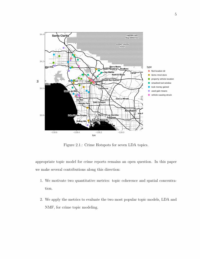
2.1 Crime Hotspots for seven LDA topics. . . . . . . . . . . . . . . . . . . . . 5

2.2 Stability over time of coherence vs generalized gini coefficient over time. . . 11

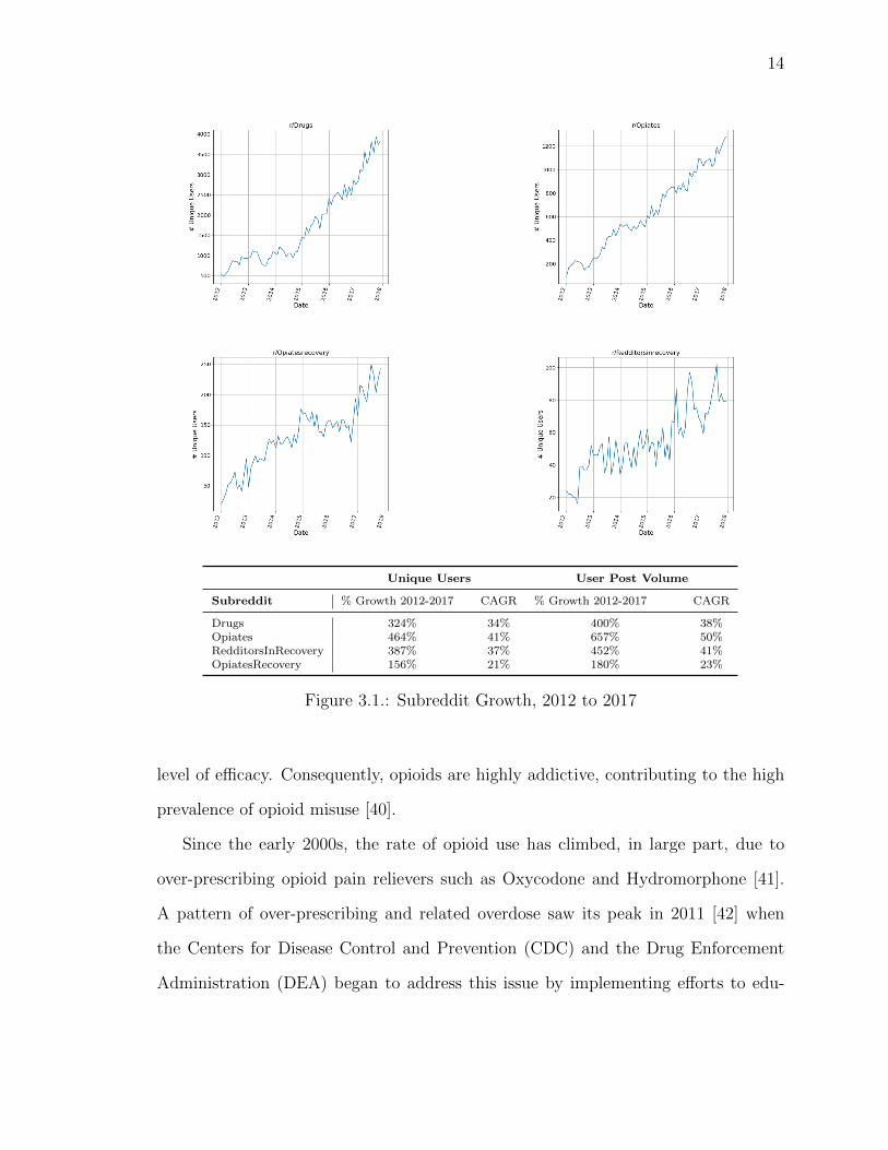
3.1 Subreddit Growth, 2012 to 2017 . . . . . . . . . . . . . . . . . . . . . . . . 14

3.2 Days Until First Recovery Post in the RECOV Group. . . . . . . . . . . . 18

3.3 Drugs with statistically significant variation in utterances between CASand CAS→RECOV (p-values < 0.05 using Kruskal-Wallis test). . . . . . . 21

3.4 Surviving One Year. Histograms showing the number of CAS and CAS→RECOV users predicted to survive at least a year. . . . . . . . . . . . . . . 27

3.5 Kaplan-Meier Curve showing surviving probability vs Days for the casestudy subject . . . . . . . . . . . . . . . . . . . . . . . . . . . . . . . . . . 28

3.6 Case Study Subject Profile . . . . . . . . . . . . . . . . . . . . . . . . . . . 29

4.1 Example knowledge graph of a homicide investigation chronology. Entitiesinclude witnesses, suspects and detectives as well as physical, documentaryand forensic type evidences. . . . . . . . . . . . . . . . . . . . . . . . . . . 33

4.2 Building knowledge sub-graphs using Named Entity Recognition and Key-word Expansion. Text and nodes are colored by its entity type (Detective-pink, Witness- green, Suspect- red, Physical evidence- yellow, Documen-tary evidence- cyan, Forensic evidence- orange, Other- gray) . . . . . . . . 44

4.3 Degree distributions of the 24 homicide investigation knowledge graphsof domain knowledge type (with and without detective nodes) and tripleextraction type (with and without detective nodes). . . . . . . . . . . . . . 45

4.4 Average number of chronology entries over first 20 weeks into the investi-gation. . . . . . . . . . . . . . . . . . . . . . . . . . . . . . . . . . . . . . . 45

4.5 Knowledge graph using Domain Knowledge Approach with and withoutdetective nodes. Each node is colored by its entity type (Detective- pink,Witness- green, Suspect- red, Physical evidence- yellow, Documentaryevidence- cyan, Forensic evidence- orange). . . . . . . . . . . . . . . . . . . 46

ix

Figure Page

4.6 Knowledge graph using Triple extraction approach with and without de-tective nodes. Each node is colored by its entity type (Detective- pink,Witness- green, Suspect- red, Physical evidence- yellow, Documentaryevidence- cyan, Forensic evidence- orange, Other- gray). . . . . . . . . . . 47

4.7 AUC and standard error for each network statistic in week 1 of the inves-tigation. . . . . . . . . . . . . . . . . . . . . . . . . . . . . . . . . . . . . . 48

4.8 AUC of GLM model (computed uses leave one out cross-validation) vs.number of weeks into the investigation. . . . . . . . . . . . . . . . . . . . 49

x

ABSTRACT

Pandey, Ritika M.S., Purdue University, August 2020. Text Mining for social harmand criminal justice applications. Major Professor: Dr. George Mohler.

Increasing rates of social harm events and plethora of text data demands the need

of employing text mining techniques not only to better understand their causes but

also to develop optimal prevention strategies. In this work, we study three social harm

issues: crime topic models, transitions into drug addiction and homicide investigation

chronologies. Topic modeling for the categorization and analysis of crime report text

allows for more nuanced categories of crime compared to official UCR categorizations.

This study has important implications in hotspot policing. We investigate the extent

to which topic models that improve coherence lead to higher levels of crime concen-

tration. We further explore the transitions into drug addiction using Reddit data. We

proposed a prediction model to classify the users’ transition from casual drug discus-

sion forum to recovery drug discussion forum and the likelihood of such transitions.

Through this study we offer insights into modern drug culture and provide tools with

potential applications in combating opioid crises. Lastly, we present a knowledge

graph based framework for homicide investigation chronologies that may aid inves-

tigators in analyzing homicide case data and also allow for post hoc analysis of key

features that determine whether a homicide is ultimately solved. For this purpose

we perform named entity recognition to determine witnesses, detectives and suspects

from chronology, use keyword expansion to identify various evidence types and fi-

nally link these entities and evidence to construct a homicide investigation knowledge

graph. We compare the performance over several choice of methodologies for these

xi

sub-tasks and analyze the association between network statistics of knowledge graph

and homicide solvability.

1

1. INTRODUCTION

Increased rates of social harm events and plethora of text-data demands the need of

employing text mining techniques not only to better understand their causes but also

to develop optimal prevention strategies. Over the past few years, the notion of social

harm has grabbed much attention. In 2007, Paddy Hillyard and Steve Tombs played

an influential role in pushing boundaries of how criminologists conceived as definition

of crime [1]. Since then social harm perspective has been contemplated as a means

to widen scope of rather narrowed approach that criminology offers [1–4].

Social harm events such as crime and drug use continue to remain a severe threat

to societies and nations across the globe. Hence, significant research efforts have

been made to underscore the utility of data mining and machine learning to address

the issue [5–16]. Moreover, text based data is ubiquitous in crime description, homi-

cide investigation and more recently online social media and discussion forums have

promoted individuals to share their addiction stories.

Our primary interest in this work is to leverage data mining and machine learning

techniques to better understand real-time, unfiltered criminal investigation and drug

addiction data with important implication in providing necessary tools for targeted

intervention.

This thesis focuses on 3 challenging problems:

• Evaluation of crime topic models: topic coherence vs spatial crime concentration

• Investigating transitions into drug addiction through text mining of reddit data

• Building knowledge graphs of homicide investigation chronologies

2

In the first problem we suggest two quantitative metrics, coherence and spatial

concentration for the evaluation of crime topic models. Topic modeling for the catego-

rization and analysis of crime report text allows for more nuanced categories of crime

compared to official UCR categorizations [8]. We investigate the extent to which

topic models that improve coherence lead to higher levels of crime concentration in

dataset of crime incidents from Los Angeles.

The second problem of the thesis focuses on gathering insights into drug use/misuse

using text snippets from users narratives obtained from Reddit. Drug addiction is de-

lineated as compulsive, continued substance use despite its negative effects. Various

online communities offer safe haven for individuals to seek advice, extend support and

share their addiction stories. We propose a binary classifier which predicts a user’s

transition from casual drug discussion forum to drug recovery forums. Additionally,

we propose a cox regression model that outputs likelihoods of such transitions. We

found how utterances of certain drugs and linguistic features play a vital role in

predicting these transitions and offer insights into modern drug culture.

The third part of the thesis discusses a framework for creating knowledge graphs

of homicide case chronologies that may aid investigators in analyzing homicide case

data and allow for post hoc analysis of the key features that determine whether a

homicide is ultimately solved. Our method consists of 1) performing named entity

recognition to determine witnesses, suspects, and detectives from chronology entries

2) using keyword expansion to identify documentary, physical, and forensic evidence

in each entry and 3) linking entities and evidence to construct a homicide investigation

knowledge graph. We compare the performance of several choices of methodologies

for these sub-tasks using homicide investigation chronologies from Los Angeles, Cali-

fornia. We then analyze the association between network statistics of the knowledge

graphs and homicide solvability.

3

1.1 Thesis Outline

The remaining of the dissertation is organized as follows: In Chapter 2, we will

suggest two metrics topic coherence and spacial concentration for evaluation of crime

topic models. In Chapter 3, we describe transitions into drug addiction through text

mining of reddit data. In Chapter 4, we describe building of knowledge graphs for

homicide investigation chronologies Finally, we summarize the dissertation in Chapter

5.

4

2. EVALUATION OF CRIME TOPIC MODELS: TOPIC

COHERENCE VERSUS SPATIAL CRIME

CONCENTRATION

2.1 Introduction

Kuang, Brantingham and Bertozzi [8] recently introduced crime topic modeling,

the application of NMF topic modeling to short (several sentence) text descriptions

accompanying crime incident reports. The idea behind crime topic modeling is that

crime categories resulting from the FBI Uniform Crime Reporting (UCR) categoriza-

tion system may lead to a loss of information and NMF topics exhibit a more nuanced

model of the text. Under the UCR system crime incidents that reflect a complex mix

of criminal behaviors are combined into one of only a few broad categories. For ex-

ample in the following two crime text reports from Los Angeles, CA, both reports

correspond to the same category (aggravated assault) despite the fact that the two

suspects exhibit different motives and behaviors.

• S APPROACHED V ON FOOT AND FOR NO APPARENT REASON

STABBED VICT IN CHEST S FLED LOC IN UNK VEH UNK DIR

• VICT WAS WALKING OBSD SUSP GRAB A TEMPERED GLASS CANDLE

HOLDER AND THROW IT AT HER HITTING HER ON THE ARM

In [8], non-negative matrix factorization is combined with hierarchical clustering

using cosine similarity to achieve a hierarchical topic model for crime incidents. While

the resulting topics are qualitatively analyzed in [8], how to evaluate and choose the

5

33.8

34.0

34.2

34.4

−118.6 −118.4 −118.2 −118.0

lon

lat

type

fled location dir

items rmvd store

property vehicle location

smashed tool window

took money gained

used gain means

vehicle causing struck

Figure 2.1.: Crime Hotspots for seven LDA topics.

appropriate topic model for crime reports remains an open question. In this paper

we make several contributions along this direction:

1. We motivate two quantitative metrics: topic coherence and spatial concentra-

tion.

2. We apply the metrics to evaluate the two most popular topic models, LDA and

NMF, for crime topic modeling.

6

3. We show that by increasing the topic coherence of crime topic models, we may

also be able to increase the spatial concentration of crime, which has important

consequences for hotspot policing.

Topic coherence is a standard metric for the quantitative evaluation of topic mod-

els and has been shown to have good correlation with human evaluations [17]. In our

methods section we describe in greater detail coherence, but informally topics have

higher coherence when co-occurring words appear more frequently in the same topic.

For example, gun and shot may co-occur together in one topic while knife and stab

may occur in a different topic.

However, there is also a significant spatial aspect to crime that has important

implications for policing. Crime is associated with the physical environment in which

it occurs, along with the behavioral and situational conditions that ultimately link

suspect to victim to place [18]. Weisburd’s law of crime concentration states that

a small proportion of the city, known as crime hotspots (see Figure 2.1), contains

the majority of criminal events [19]. Place based interventions in crime hotspots are

known to lead to crime reductions in those areas and allow police to focus limited

resources on a small area of the city [20]. Our hypothesis is that crime topics that

have greater coherence may also have higher levels of crime concentration, facilitating

more effective policing interventions. Referencing the two assault reports above, a

topic corresponding to the first report may necessitate a gang intervention task force

whereas the second report may belong to a mental health topic. These two topics

may individually be more concentrated in space compared to when combined.

2.2 Methods

Latent Dirichlet Allocation (LDA) is a Bayesian graphical model for text doc-

ument collections represented by bag-of-words [17] [21]. LDA is given by a generative

7

probabilistic model, where each word in a document is generated by sampling a topic

from a multinomial distribution with Dirichlet prior and then sampling a word from

a separate multinomial with parameters determined by the topic.

Non-negative matrix factorization (NMF) is a widely used tool for the anal-

ysis of high-dimensional data as it automatically extracts sparse and meaningful

features from a set of nonnegative data vectors [22]. NMF uncovers major hidden

themes by factoring the term-document matrix of a corpus into the product of two

non-negative matrices, one of them representing the relationship between words and

topics and the other one representing the relationship between topics and documents

in the latent score topic space [23].

Coherence is a quantitative measure of the similarity of words in a topic. In

particular, given a set V of topic words in a corpus (we will use the top 10 most

frequent words in each topic), coherence is computed as a sum of similarity scores

over all pairs of words in V . While different similarity scores may be used, we consider

the intrinsic measure UMass [24] to calculate the coherence. The Umass similarity

score measures the extent to which words tend to co-occur in topics together:

score(wi, wj) = logD(wi, wj) + ε

D(wj)

where D(wi, wj) is the number of documents containing both words wi and wj and

D(wj) is the number of documents containing word wj.

Gini index in the context of crime, is a measure of the extent to which a large

percentage of crime falls within a small area percentage of a city [25] [26]. Consider a

city divided into grid cells where the amount of crime falling in each cell is calculated

over an observation period. The Lorenz curve is computed by rank ordering the cells

by count and then plotting the cumulative percentage of crime against the cumulative

percentage of land area. The Gini index, G, ranges from 0 to 1 and is the ratio of

8

the line of equality (representing equal hotspots across the city) and the area under

the Lorenz curve. In particular, G = 0 corresponds to equal distribution of crime at

all grid cells and G = 1 corresponds to maximal concentration at a single hotspot.

Since, the number of crimes may be less than the number of places, we measure the

crime concentration using an adjusted gini coefficient G′, defined as the area between

the Lorenz curve and line of maximal equality [25],

G′ = max(1

c,

1

n)(2 ∗

n∑i=1

iyi − n− 1)−max(n

c, 1) + 1

where c is the total number of crimes, n is the total number of places, yi is the

proportion of crimes occurring in place i and, i is the rank order of the place when

places are ordered by the number of crimes yi.

2.3 Results

We analyze a data set of crime incidents in Los Angeles that spans the years

2009 to 2014. Each incident is accompanied by a date, latitude, longitude, and text

description of the incident that is a short paragraph. For measuring the Gini index,

we divide Los Angeles into a grid of size 100x100 and measure the number of crimes

of each topic falling in each grid cell.

As part of text preprocessing we remove stop words [27]. We extend the stop-words

list from the python NLTK package with common words such as victim, suspect and

unknown. We discard all the stop-words and any word whose length is less than 3

characters. We then process the document term matrix using Term Frequency Inverse

Document Frequency (TFIDF) weighting factors [28] to emphasize words that occur

frequently, but penalizing words that occur in a large percentage of documents (for

example stop words not found in our annotated list).

9

For each year, we sample a balanced data set of 35,000 events, 5000 events from

each of seven UCR categories: vandalism, theft, burglary theft from vehicle, burglary,

robbery, aggravated assault, and other. We then estimate LDA and NMF using k = 7

topics each for a fair comparison to the UCR categories.

Table 2.1.: Coherence vs. spatial concentration 2009-2014

type coherence std. error gini std. error

category -0.817 0.0068 0.3308 0.0021lda -0.287 0.031 0.360 0.007nmf -0.300 0.012 0.308 0.002

In Table I we present the average coherence across years along with the average

Gini coefficient. We use a weighted average where the average is weighted by the

number of events in each category to take into account the fact that some topics may

have more or less than 5000 events. Here we see that LDA has both the highest

coherence of topics and highest gini coefficient. In Table II we display the most

frequent words of each UCR crime category in 2014 and in Table III we display the

same table for LDA topics in 2014. For example, the burglary theft from vehicle

(BTFV) category has a coherence value of -.672 and a gini index of .282. The closest

topic of LDA to BTFV is topic 5, however this topic has higher coherence of -.462

and a higher gini index of .39. There are several topics where LDA has a lower gini

index, for example in the case of theft. These topics with lower gini index have lower

number of events, resulting in more zero count cells, and the adjusted gini index is

lower in these cases. However, in the weighted average across topics LDA has a higher

over all gini index.

In Figure 2 we display coherence and the gini coefficient over time to assess the

stability of these results. Here we see that LDA consistently has a higher gini index

10

Table 2.2.: Category 2014

coh. gini frequent words

-0.810 0.320 used location fled vehicle info face verbal without punched became-0.892 0.296 vehicle fled location window used causing door damage side smashed-0.883 0.433 property location fled removed took store entered items without paying-0.672 0.282 vehicle property location fled removed window entered took smashed door-0.720 0.364 prop. fled approach location took vehicle demand money removed punch-0.894 0.257 location property fled door entered removed window open rear entry-0.825 0.353 vehicle fled location struck head hit verbal knife causing argument

over time. For some years NMF has a higher coherence, though both NMF and LDA

have consistently higher coherence than the UCR crime categories.

Table 2.3.: LDA 2014

coh. gini frequent words

0.000 0.467 items rmvd store phone paying business exited selected cell concealed-0.122 0.146 used gain means smash open remove merchandise permission card ifo0.000 0.180 took money gained secured returned parked demanded missing stated gave-0.231 0.377 vehicle causing struck punched approached face head property verbal times-0.462 0.390 property vehicle location removed entered door window rear entry ransacked-0.185 0.346 fled location dir direction resid hit entered approached foot open-0.254 0.163 smashed tool window open residence pushed res pry produced glass

2.4 Conclusion

We suggested two performance metrics for crime topic models: topic coherence and

the gini coefficient for measuring spatial concentration. We showed that the choice of

topic model has important implications for detecting crime hotspots. In particular,

it is possible to achieve more coherent topics that simultaneously concentrate to a

higher degree in space, allowing for more targeted police interventions given limited

resources. For the data set analyzed in Los Angeles, our results show that LDA

has the highest coherence and gini coefficient compared to NMF and UCR crime

categories.

11

Future research may focus on the joint optimization of coherence and spatial

concentration. LDA and NMF in this paper were provided with no spatial informa-

tion. Methods may be developed that can improve both coherence and concentration

jointly using supervised learning. Additionally, such methods may be extended to

spatio-temporal models where topics and spatial hotspots evolve over time [29].

0.300

0.325

0.350

0.375

2009 2010 2011 2012 2013 2014

year

gini

type

category

lda

nmf

−0.8

−0.6

−0.4

−0.2

2009 2010 2011 2012 2013 2014

year

cohe

renc

e type

category

lda

nmf

Figure 2.2.: Stability over time of coherence vs generalized gini coefficient over time.

12

3. REDDITORS IN RECOVERY: TEXT MINING

REDDIT TO INVESTIGATE TRANSITIONS INTO DRUG

ADDICTION

3.1 Introduction

The rate of nonmedical opioid use has increased markedly since the early 2000s.

While recent efforts have been made to curb over-prescribing [30, 31], morbidity and

mortality rates associated with opioid misuse continue to worsen [32]. Traditionally,

those suffering from addiction take to support groups, such as Alcoholics Anony-

mous (AA) and Narcotics Anonymous (NA), on their road to recovery [33]. These

groups, which provide an encouraging community and facilitate programs for addic-

tion management and recovery, have shown significant promise in assisting substance

abusers [34]. In addition to the aforementioned support groups, federal support is

provided through organizations such as the Substance Abuse and Mental Health Ser-

vices Administration (SAMHSA). Among others, SAMHSA offers programs such as

Medication-assisted Treatment and Too Smart To Start - the former combines the

use of medication and behavioral therapy in the treatment of substance abuse and

the latter is a public education initiative which deters underage alcohol use.

More recently, communities have been established in online social media and dis-

cussion forums including Reddit, MedHelp, Twitter and Drugs-Forums.com, among

others. Enacted and internal stigmatization addicts must face [35,36] in conjunction

with the convenience, privacy, and anonymity of such online communities may be ex-

planations for their rapid expansion. These online hubs offer havens for individuals to

13

seek advice, extend support, and share their addiction stories without fear of recourse

or judgment. A previous study suggested that these communities can be tremendous

resources in the understanding, monitoring and intervening of substance abuse [37].

Earlier works underscore the utility of mining data from social media sites to un-

derstanding trends of human health and drug use [9, 11–13, 38, 39]; however, most

of these works do not explore the particular transition from voluntary drug use to

compulsive drug use, as well as the various factors that influence such a transition.

Our research leverages machine learning and data mining techniques to better under-

stand real-time, unfiltered user data presented to us via Reddit, and in particular,

focuses on the understanding of how users transition into addiction can be predicted

by using drug utterances and linguistic features contained in their Reddit posts. We

present two statistical models: 1) a “transition classifier” that predicts if a user, given

6 months of content history in general drug discussion forums, will post in forums

dedicated to substance recovery support in the subsequent 12 months and 2) a pro-

portional hazards survival model which estimates a user’s probability of posting in a

recovery forum within the next year.

3.2 Background and Related Works

3.2.1 Drug Addiction and the Opioid Crisis

Drug addiction is characterized by the compulsive, continued use of a substance

despite its negative effects. While drug consumption often begins as recreational,

frequent use increases one’s tolerance, ultimately altering brain chemistry, inducing

heightened desires for drugs, and prompting involuntary and compulsive use. Opioids

readily increase tolerance; with each use, one requires larger doses to reach the same

14

Unique Users User Post Volume

Subreddit % Growth 2012-2017 CAGR % Growth 2012-2017 CAGR

Drugs 324% 34% 400% 38%Opiates 464% 41% 657% 50%RedditorsInRecovery 387% 37% 452% 41%OpiatesRecovery 156% 21% 180% 23%

Figure 3.1.: Subreddit Growth, 2012 to 2017

level of efficacy. Consequently, opioids are highly addictive, contributing to the high

prevalence of opioid misuse [40].

Since the early 2000s, the rate of opioid use has climbed, in large part, due to

over-prescribing opioid pain relievers such as Oxycodone and Hydromorphone [41].

A pattern of over-prescribing and related overdose saw its peak in 2011 [42] when

the Centers for Disease Control and Prevention (CDC) and the Drug Enforcement

Administration (DEA) began to address this issue by implementing efforts to edu-

15

cate both medical professionals and the public on appropriate opiate use [40]. These

efforts included tightening prescriptions and developing new prescription opioids that

are “abuse-deterrent” [40]. While these efforts were met with declines in prescription

opioid abuse, illicit opioid use—including that of Heroin and Fentanyl—continued

to increase and contribute to rising opioid-related injuries and overdoses [42]. One

explanation for the continued rise in illicit opioids was supposedly that increased

barriers to medication prompted chronic pain patients to supplement their reduced

prescription allowance via self-medication, further exacerbating opioid-use risk [42].

Since Heroin is pharmacologically similar to prescription opioids, relatively cheap, and

readily available, it was an obvious replacement for those previously using prescription

opioids [41]. The trends outlined here demonstrate the need for balanced prevention

measures that aim to reduce opioid abuse and overdose while simultaneously main-

taining access to prescription opioids and treatment programs as needed [40].

3.2.2 Using Social Media to Understand Drug-Related Issues

Mining social media data to study health and drug-related behavior is not a new

concept. MacLean et al. created a model from MedHelp forums that attempts to

predict addiction relapse [13]. Paul and Dredze used a factorial LDA topic model on

forums from Drugs-Forums.com to model drug types, delivery methods, and other

related aspects such as cultural and health factors in the context of recreational drug

use [38]. Sarker et al. assessed the use of Twitter in analyzing patterns of drug abuse,

and built a binary classifier that distinguishes whether or not a tweet contains signs of

medication abuse [39]. Other studies have applied machine learning to classify users

of an addiction recovery mobile application [12] and to identify distinct behavioral

markers between Heroin and amphetamine dependence [43]. In the context of Reddit,

Choudhury et al. used Reddit data to explore the transition between mental health

16

discourse and suicidal ideation, and built a classifier that distinguishes between those

two states [9]. Eshleman et al. demonstrated the possibility of using a binary classifier

in predicting a user’s propensity to post in a recovery-related subreddit [11]. Our

research expands upon this latter work by exploring various linguistic factors and

drug utterances in a user’s post that are predictive of transitions into substance

abuse; further, we build a survival model capable of estimating the probability of

such transitions, providing deeper insight into the explanatory factors involved in

such shifts.

3.3 Reddit Data

Reddit.com (or Reddit) is an online collection of threads grouped by user com-

munities known as “subreddits” with each covering a distinct topic. Reddit users, or

“Redditors,” subscribe and submit content to subreddits which interest them, and

have their submitted content voted and commented on by fellow Redditors. Reddit

has the added appeal of anonymity, allowing users to partake in unfiltered conversa-

tions on topics of shared interest. As of April 2018, the platform has over 330 million

active users with 130 thousand active subreddits [44].

Threads on Reddit are defined by a user’s initial post and the subsequent com-

ments on the post by other users. Posts typically discuss a user’s own substance

use/abuse while comments primarily answer questions asked in the post and/or offer

support to the post author. Since our objective is to learn about transitions into sub-

stance abuse, which requires analysis of content pertaining to a user’s own situation,

we restrict our analysis solely to posts.

Using the pushift.io Reddit API1, we pulled data from January 2012 through May

2018. This dataset consisted of 309,528 posts from 125,194 unique users and included

1https://pushshift.io/

17

various attributes of each post such as content, title, author, date of post, number

of comments, and number of upvotes. We focus on four major drug-related subred-

dits: r/Opiates, r/Drugs, r/OpiatesRecovery, r/RedditorsInRecovery. In addition to

having adequate user and post volume, these subreddits host discussions on a vari-

ety of drugs. Whereas r/Opiates and r/Drugs primarily serve as forums for general

drug discussion, which tend to be more casual in nature, the r/OpiatesRecovery and

r/RedditorsInRecovery subreddits provide an avenue for those struggling with sub-

stance abuse and addiction to seek advice, share success and relapse stories, and

support others. The measurable growth in both user base and post volume be-

tween 2012 and 2017 is exhibited in Figure 3.1. In the proceeding analyses, we

will refer to r/Opiates and r/Drugs as “casual” subreddits and r/OpiatesRecovery

and r/RedditorsInRecovery as “recovery” subreddits.

3.4 Transition Classification: Modelling Transitions from Recreational

Use to Substance Abuse

We trained a binary classifier to model whether a user who posts only in casual

subreddits in their first 6 months will eventually go on to post in recovery subreddits

in the following 12 months.

3.4.1 Creating Classes

Analysis was restricted to users with at least 3 posts and who exclusively posted

in casual subreddits in their first 6 months on Reddit. Of these, we found the subset

of users that posted in a recovery subreddit within the next 12 months; there are

220 such users, and we label this group collectively as the CAS→RECOV class.

18

Figure 3.2 shows the distribution of the number of days until the first recovery post

for the CAS→RECOV group.

Figure 3.2.: Days Until First Recovery Post in the RECOV Group.

There are 2,836 users with at least 18 months of casual-only posts. To maintain

balance between the two classes, we randomly sample 220 users from this set to form

the CAS class. We then split these 440 examples into a training set (352 users) and

test set (88 users).

3.4.2 Feature Selection

In applying a machine learning model for predicting users’ transition from CAS→

RECOV, each user should be represented by a vector. For this purpose, we extract

various features from a user’s posts, including dense embedding vectors obtained

through Doc2V ec, linguistic characteristics of user posts, and drug utterances in the

post. For the last two kinds of features, we use Kruskal-Wallis statistical test to

determine which drug utterances and linguistic measures are significantly different

between the CAS and CAS→RECOV classes. Tables ?? and ?? show the selected

features and their frequency distribution.

19

Doc2Vec Embeddings. Text clustering and language processing applications

involve algorithms that generally require the input text data to be represented as

a fix-length vector. Bag-of-word models and n-gram models are often utilized to

generate these vector representations due to their simplicity, but both lack contextual

information. We therefore use Gensim’s Doc2Vec model to create 100-dimensional

vector representations for each user post [45]. The idea behind such representations

was first proposed by Le and Mikolov [46], who sought to create a methodology

that generates vector embeddings for texts of variable length. This unsupervised

framework has been shown to outperform the bag-of-words and N-gram models in

sentiment analysis and other information processing tasks.

Since predictions are based on 6 months of user posts, we aggregate the document

vectors of a user’s posts over this period. Let Dj be the set of posts made by user j in

the first 6 months on Reddit (ordered by date). Then, denoting the ith post of user j

by dji , we use the centroid of the doc2vec vectors of user j’s posts as a representation

of the user j.

Cj =1

|Dj|

|Dj |∑i=1

dji ∈ R100

In the above equation, dji is the doc2vec based vector representation of dji . Though

simplistic, prior works [47, 48] have suggested the efficacy of using the centroid of

document representations to capture meaningful content from a set of documents.

Linguistic Measures. The specific language and words one employs in speech

and writing can reveal much about one’s psychological and social states [49,50]. Fur-

ther, studies have shown socio-psychological and personality differences between drug

and non-drug addicts [51]. To capture both linguistic components (e.g. fraction of

pronouns, verbs, and articles among others) and psychological aspects (e.g. words

20

associated with positive/negative emotions, anger, and family/friends among others)

of user posts, we use the Linguistic Inquiry and Word Count2 (LIWC), a text analysis

program that categorizes words into 93 groups which reflect different emotions, think-

ing styles, social concerns, and parts of speech. Though LIWC variables capture more

than purely linguistic dimensions of texts, we will use the phrases “LIWC features”

and “linguistic features” interchangeably hereafter for simplicity.

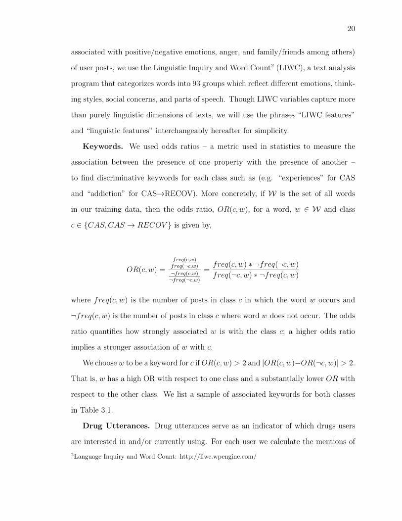
Keywords. We used odds ratios – a metric used in statistics to measure the

association between the presence of one property with the presence of another –

to find discriminative keywords for each class such as (e.g. “experiences” for CAS

and “addiction” for CAS→RECOV). More concretely, if W is the set of all words

in our training data, then the odds ratio, OR(c, w), for a word, w ∈ W and class

c ∈ {CAS,CAS → RECOV } is given by,

OR(c, w) =

freq(c,w)freq(¬c,w)

¬freq(c,w)¬freq(¬c,w)

=freq(c, w) ∗ ¬freq(¬c, w)

freq(¬c, w) ∗ ¬freq(c, w)

where freq(c, w) is the number of posts in class c in which the word w occurs and

¬freq(c, w) is the number of posts in class c where word w does not occur. The odds

ratio quantifies how strongly associated w is with the class c; a higher odds ratio

implies a stronger association of w with c.

We choose w to be a keyword for c ifOR(c, w) > 2 and |OR(c, w)−OR(¬c, w)| > 2.

That is, w has a high OR with respect to one class and a substantially lower OR with

respect to the other class. We list a sample of associated keywords for both classes

in Table 3.1.

Drug Utterances. Drug utterances serve as an indicator of which drugs users

are interested in and/or currently using. For each user we calculate the mentions of

2Language Inquiry and Word Count: http://liwc.wpengine.com/

21

Table 3.1.: Discriminatory keywords for CAS and CAS→RECOV class using OddsRatio

Class Keywords

CAS friends, completely, lsd, trip, reddit, music, weird, dr, friend,experiences, ended, 100, mdma

CAS→RECOV quit, addiction, clean, anymore, subs, suboxone, oxy, bupe

each drug (as a % of all drugs they mention). This calculation includes both formal

drug names of the drug, colloquial (“street”) names, and major brand names (e.g.,

OxyContin® is a common brand of oxycodone and “coke” is a oft-used name for

cocaine). In Figure 3.3, we displays four drugs that have highly significant variation

in utterance between the two classes.

Figure 3.3.: Drugs with statistically significant variation in utterances between CASand CAS→RECOV (p-values < 0.05 using Kruskal-Wallis test).

22

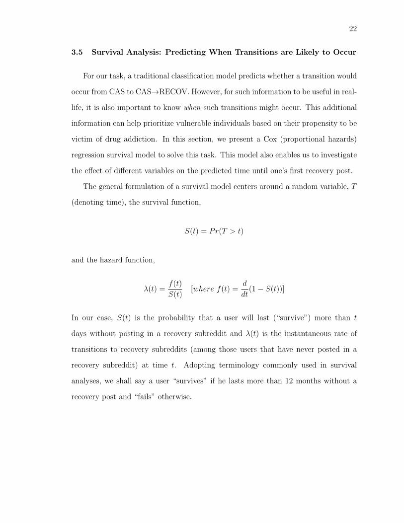
3.5 Survival Analysis: Predicting When Transitions are Likely to Occur

For our task, a traditional classification model predicts whether a transition would

occur from CAS to CAS→RECOV. However, for such information to be useful in real-

life, it is also important to know when such transitions might occur. This additional

information can help prioritize vulnerable individuals based on their propensity to be

victim of drug addiction. In this section, we present a Cox (proportional hazards)

regression survival model to solve this task. This model also enables us to investigate

the effect of different variables on the predicted time until one’s first recovery post.

The general formulation of a survival model centers around a random variable, T

(denoting time), the survival function,

S(t) = Pr(T > t)

and the hazard function,

λ(t) =f(t)

S(t)[where f(t) =

d

dt(1− S(t))]

In our case, S(t) is the probability that a user will last (“survive”) more than t

days without posting in a recovery subreddit and λ(t) is the instantaneous rate of

transitions to recovery subreddits (among those users that have never posted in a

recovery subreddit) at time t. Adopting terminology commonly used in survival

analyses, we shall say a user “survives” if he lasts more than 12 months without a

recovery post and “fails” otherwise.

23

3.5.1 Right-Censored Data

Besides providing the answer whether a user will survive beyond a given time,

survival model has another crucial advantage: a survival model can utilize “censored

data” effectively, whereas a traditional regression model fails to do so. Censored data

(also known as right-censored data) refers to observations for which the desired event

has not happened yet. For instance, say, the end of observation time for our study is

t. Now, if a user has never posted in recovery forum within our observation period,

one does not know with certainty whether that user will not post in recovery on some

day t > t. This is an example of right-censored data instances.

Our model requires users to have at least 10 posts where the first 3 were casual

and not all occurring on the same day. This criteria eliminates the case of 0-day

survival times, which in real-life makes little sense. In our dataset, there are 2,367

users satisfying these restrictions, and for each user, we look only at (up to) their

first 12 months of posts. 165 of these users fail within the first 12 months, while the

remainder are right-censored observations.

3.5.2 Cox Regression

A Cox regression model is a specific type of survival model that accounts for

the effects of covariates on some baseline hazard function λ0(t). Formally, if we let

x(i) ∈ Rd be a column vector of features for user i, the hazard for user i is,

λi(t) = λ0(t) exp{xᵀβ(i)}

and the corresponding survival function is,

Si(t) = S0(t)exp{βᵀx(i)}

24

where β ∈ Rd is a vector of trainable parameters. The data for the model can be

denoted Dsurv = {(yi, δi, x(i)) : i = 1, 2..., n} where yi is the minimum of the censoring

time Ci (end of observation time) and survival time Ti and

δi =

1 if Ti = yi

0 otherwise

,

where δi denotes whether or not an instance is censored. We train β by maximizing

the partial likelihood estimate (under iid assumption),

L(β|Dsurv) =∏n

i=1

[λ0(t) exp{βᵀx(i)}∑

j∈Ψ(yi)λ0(t) exp{βᵀx(j)}

]δi

where Ψ(t) = {i : yi > t} is the subset of users who survive past time t.

3.6 Results

In this section we provide experimental results for both binary classification and

cox regression. Results for both models suggest that drug utterances and linguistic

features can be indicative of one’s propensity to shift towards substance abuse.

We use categorical accuracy and F1 score to evaluate the transition classifier. A

baseline model, which used only Doc2Vec embeddings, achieved a modest 69.3% test-

set accuracy. With the inclusion of LIWC linguistic features, drug utterances, and

class-specific keywords in addition to tuning model parameters through grid search,

we improved accuracy by roughly 5% (Table 3.2).

Performance of the survival model was evaluated using Concordance Index (C-

Index), a standard metric often employed in survival models [52]. Concordance ranges

from 0 to 1 (a higher score indicates a stronger model) and is analagous to the AUC

25

Table 3.2.: Transition Classifier Results Summary. Table displays test-set performanceof Random Forest with 170 trees (selected using grid search and 10-fold cross validation)using different features. Model trained on users’ first 6 months of posts and predicts tran-sitions in the subsequent 12 months. Number of train and test set examples were 352 and88, respectively.

Model Accuracy F1 Score

Doc2Vec 0.693 0.682LIWC 0.659 0.659Doc2Vec + drugs + keywords 0.716 0.725LIWC + drugs + keywords 0.739 0.736Doc2Vec + LIWC + drugs + keywords 0.750 0.750

score of the Receiver Operating Characteristic (ROC). Our best Cox model achieved

a 0.823 C-Index on the test-set (Table 3.3), indicating a moderately strong model.

Table 3.3.: Cox Model Results Summary. Train/test split of 1,775 (1665 censored) and592 (352 censored) users, respectively. C-Index shown for models using different featuresets. The model using drug utterances, keywords, and LIWC features performed best ontraining set using 5-fold cross validation and gave a test-set C-Index of 0.820. Test set dataconsisted of 45 observed and 592 censored examples.

Model C-Index

Doc2Vec 0.790Doc2Vec + drugs + keywords + LIWC 0.788Drugs + keywords + LIWC 0.820

Test Set Performance 0.820

In addition to training Cox models using different feature sets, we sought to ex-

plore the explanatory strength of individual covariates by fitting a model to each

individual feature (Table 3.4 presents the C-statistics from this experiment). Using

this approach, we found that utterances of drugs such as Buprenorphine, Heroin, and

LSD, have a stronger impact on a user’s predicted survival probability relative to

other drugs. This is in accordance with our earlier analysis (Figure 3.3). Similarly,

LIWC dimensions such as “leisure,” “time,” and “focuspresent” have relatively more

26

predictive power (Table 3.4). These features measure the extent to which posts con-

tain terms related to leisure activities (e.g. “cook,” “chat,” “movie”), time-related

terms (e.g. “hour,” “day,” “oclock”), and terms that indicate a focus on the present

(e.g “today,” “is,” “now”).

Table 3.4.: Top 10 Explanatory Covariates

Drug Name C-Index

Heroin 0.748Buprenorphine 0.702

LSD 0.687psilocybin 0.628oxycodone 0.623marijuana 0.621Ecstasy 0.614fentanyl 0.610

oxymorphone 0.608amphetamine 0.597

LIWC feature C-Index

leisure 0.668Period 0.646time 0.646

ingest 0.645informal 0.642netspeak 0.633

focuspresent 0.630relativ 0.627nonflu 0.612money 0.610

3.6.1 Survival Predictions on the Transition Dataset

We looked once again at the 220 CAS and 220 CAS→RECOV Redditors, this

time through the lens of our trained survival model. In Figure 3.4, we fix the time

duration at 12 months and compare survival probabilities between the two groups.

Not surprisingly, a sizable majority of the CAS group have high probability (> 90%)

of surviving past 12 months. We then approximated the addictive potential of certain

drugs by measuring the average survival probability of users who share a common

drug of choice. For example, we found that users whose top drug utterances were

Ecstasy or LSD had high probability of surviving while users whose drug of choice is

Heroin or Buprenorphine had a comparatively smaller chance of surviving (Table 3.5).

27

Figure 3.4.: Surviving One Year. Histograms showing the number of CAS and CAS→RECOV users predicted to survive at least a year.

Table 3.5.: One-Year Survival Probability by Top Drug Mention

Drug Name Surv. Prob. Drug Name Surv. Prob.

Ecstasy 0.987 fentanyl 0.820LSD 0.981 cocaine 0.774

benzodiazepines 0.877 oxycodone 0.767marijuana 0.872 Heroin 0.502

methamphetamine 0.824 Buprenorphine 0.498

3.7 Case Study

In this section, we illustrate one of several potential uses of our models by applying

them to an actual Redditor. Figure 6 presents a profile of the user including a redacted

sample of his writing, the most prevalent LIWC aspects, and most uttered drugs from

his posts.

The subject is a routine user of Heroin and an active participant in r/Opiates.

His top 3 drug utterances are Heroin, oxycodone, and Buprenorphine with Heroin

representing approximately 35% of his total drug mentions. Referring to Table 3.5,

one may expect a lower 12-month survival probability for this user relative to someone

with a random drug composition. Furthermore, LIWC dimensions of the subject’s

posts are consistent with Redditors who do not survive 1 year. For example, users

28

who fail tend to have a lower “focuspresent” dimension, and our subject scores close

to the 75th-percentile in this category (Table ??).

3.7.1 Model Predictions of Subject

Given the subject’s background and profile, it is encouraging that our transition

classifier labels him as CAS→RECOV. That is, using only the subject’s first 6 months

of casual posts, the classifier predicts he will post in recovery within the subsequent

12 months. Furthermore, our Cox model predicts a less than a 18.6% chance he will

survive past 1 year (Figure 3.5), indicative of a high-risk user. Consulting the subject’s

entire post history, we found that he did eventually post in r/OpiatesRecovery 200

days after his first post.

Figure 3.5.: Kaplan-Meier Curve showing surviving probability vs Days for the casestudy subject

3.8 Discussion

In this work, we explored transitions from recreational substance use to substance

abuse using survival analysis and binary classification. In our classifier, we were able

to predict whether a previously “casual” user will post in a recovery subreddit within

the next 12 months. Using our survival model, we were able to uncover distinct

29

Initial Posts

Finished my stash off this morning as was expecting to havemore by now. Just had a call..... Its not good. Hopefullytomorrow he said. HOPEFULLY..... Tonight is going to bea very long night for me.

...Ran out of dope last night, meaning to get more this morn-ing. My man was out so planned on getting it while at work.But, I forgot my cash. DAMN, I have a whole night shift infront of me while starting to get sick. This sucks. Hope yourall having a better night than me.

...I have aquired 15 x 100mcg Fent patches of the matrixtype. I figured I would try smoking a bit of one and...I nowknow why its so easy to OD on them....Gonna be super carefulwith them though, lost 2 good friends over the years throughfent OD’s. Will keep posting at least once a day until theirgone though. Happy nods ppl, and keep safe.

First Recovery Post

Hi guys, I figured this would be asgood a place as any to post mystory, and look for answers. I havebeen using Heroin on and off forabout some years now...I am pastthe physical withdrawals now, butstill really struggling with the psy-chological side...All my friends use,hell, most people I know use. I wantto stop for my wife and son aboveeverything else, bit finding it reallyhard. So, what advice do you guyshave. Any will be greatly appreci-ated. I’m guessing I just want some-one to talk to as today I am reallystruggling with it. Thanks

LIWC Avg. Value LIWC Avg. Value

Authentic 71.261 netspeak 2.176relativ 16.059 percept 2.028focuspresent 13.495 leisure 1.189Period 11.902 money 0.862WPS 10.648 family 0.629Sixltr 9.534 nonflu 0.579time 8.281 sad 0.344conj 5.841 death 0.234informal 4.130 ingest 0.215insight 2.491 Exclam 0.000

(a) Subset of LIWC

(b) Top Drugs

Figure 3.6.: Case Study Subject Profile

features such as specific drug utterances and linguistic features of a given post that

influence a given user’s probability of transitioning from recreational substance use

to substance abuse. In this section, we discuss the implications of these results in

informing drug use culture and possible methods of drug classifications, as well as

highlight potential applications of our models in understanding drug use from the

user’s perspective.

30

3.8.1 Informing Culture and Classifications

Based on our Redditors’ posts, a pattern of use was apparent: drugs such as LSD,

Ecstasy, marijuana, and alcohol were often used by Redditors attending parties, music

festivals, or social events in general. In contrast, opioids were commonly used as a

habitual, lone activity or in smaller, low-energy gatherings. This trend learned by

inspection was further supported by post-level analyses showing a co-occurrence of

frequent mentions of LSD and Ecstasy and frequent use of words such as “music,”

“rave, ” and “party.” Paul and Dredze found similar results in their use of topic

modeling to understand various factors, including the cultural factors, associated

with certain drug use. For example, the “culture” words associated with Ecstasy

include [“music”, “people”, “great”, “rave”], while the “culture” words associated

with opioids include [“life”, “years”, “money”, “time”, “shit”] [38].

Our survival model suggests that certain drug utterances were highly explanatory

in influencing the probability of substance abuse – for instance, a user with higher

Heroin mentions (as a percentage of total drug mentions) is associated with a higher

probability of substance abuse, while higher LSD and Ecstasy mentions are asso-

ciated with lower probabilities. This particular example directly conflicts with the

current national drug classifications outlined by the DEA, who classifies drugs into

five “schedules” based on their dependence potential as well as the level of accepted

medical use. As it currently stands, drugs including Heroin, LSD, marijuana, and

Ecstasy are classified as Schedule I, while most other opioids along with cocaine are

classified as Schedule II. Our models, however, suggest that the drugs of choice for

individuals who are likely to transition are often not the drugs labeled as Schedule I,

with the exception of Heroin. Table 3.5 outlines the average “survival” probabilities

associated with drugs common among our users. In our model, users whose drugs of

choice are Ecstasy, LSD, and marijuana have a higher predicted survival rate which

31

may suggest that these drugs could be better classified as Schedule II or lower. Sim-

ilarly, their lower associated survival probabilities may be justification for a higher

classification for drugs like Buprenorphine, oxycodone, and cocaine.

Other studies have reached similar conclusions. The United Kingdom has similar

drug classifications based on addictive potential, and places many of the Schedule I

drugs as their top dangerous drugs as well. Yet Nutt and colleagues [53] found that

the UK system of classification is somewhat arbitrary and not driven by scientific

evidence. In their work, they reclassified the drugs listed in the UK’s guidelines

using potential of harms of individual drugs, and found that the top drugs with

high potential of harm include Heroin, cocaine, barbiturates, street methadone, and

ketamine. Their findings also disagree with UK’s designation of LSD and Ecstasy

in the top drug class – this aligns with our results and further suggests the higher

potential of harm from opioids relative to these other drugs.

Similarly, Sarvet et al [54] discuss the increasing amount of evidence in support of

the therapeutic properties of medical marijuana. According to them, medical experts,

including the American Medical Association, have urged the DEA to reschedule mar-

ijuana from Schedule I to Schedule II. They argue that not only would it increase

access for patients who could benefit from this form of treatment, it would also enable

further research and development of cannabinoid-based medicine.

3.8.2 Limitations

In this section, we list some limitations to our work: 1) We identify selection bias

in our Redditors, as they are choosing to express their opinions on Reddit and are

likely much more open about their drug use/recovery progress. Since this may not

be indicative of all drug users, our results may not be generalizable to the larger

population. 2) We use participation in general drug forums and recovery forums as

32

proxies for recreational use and substance abuse, respectively. However, since there

are no rules preventing abuse-related posts in our casual subreddits, these subreddits,

though predominately about casual drug discussion, do contain abuse-related posts.

3) We cannot make any clinical disgnoses of drug addition or mental illness based

solely on our analyses. 4) Although we made attempts to include all forms of drug

names in our drug counts, there may be names that are not included, and thus we may

not have captured all types of drug utterances. 5) Our research uncovers certain post-

level characteristics that influence the likelihood of transitions into recovery subreddits

but cannot explain why Redditors make these transitions.

Despite these limitations, our findings provide unique insight into drug use pat-

terns from the perspective of users and uncovered features within one’s posts that

may be predictive of future substance abuse. Our work demonstrates the utility of

online forums and social media sources in understanding human health and activity.

Finally, the computational models that we provide can be utilized into real-life ap-

plications. For example, there can be a software App for Redditors in which they

input their posts and the App returns the poster’s propensity for drug abuse. Also,

this App can be used as a predictive device to help counselors and psychologists in

advising their patients.

3.9 Future Work

Further research in this area could focus more on the temporal aspect of a user’s

post sequence. Similar to the work done by Maclean et al. [13], which used a Con-

ditional Random Field (CRF) to model phases of addiction, one could construct a

sequence model using our subreddits to track users’ phases of “pre-addiction” to

further analyze transitions into addiction and uncover more contextual factors that

influence such transitions. We hope to explore such analysis in the future.

33

4. BUILDING KNOWLEDGE GRAPHS OF HOMICIDE

INVESTIGATION CHRONOLOGIES

4.1 Introduction

A large amount of text-based data is produced during a homicide investigation

including basic descriptions of the event, evidence logs, forensic reports, maps and

annotated photographs, and transcripts of investigator’s notes and witness interviews.

These data are compiled into a so-called “Murder Book” that summarizes the paper

trail from the time the incident was reported to the time a case is closed.

In the United States nationally, around 60% of homicides are solved or cleared

via arrest or other exceptional means such as death of the offender [55]. Several

WIT1

VICT

WIT2

SUS1

photograph

WIT3

murder

WIT4

WIT5

WIT6

WIT7

WIT8

WIT9

handgun

SUS2

WIT10

WIT11

crime

scene

gunshot

wounds

report

notes

caliber

casings

body

vehicle

photos

SUS3

security

cameras

recording

firearm

recorded

WIT12

property

Figure 4.1.: Example knowledge graph of a homicide investigation chronology. Enti-ties include witnesses, suspects and detectives as well as physical, documentary andforensic type evidences.

34

factors appear to play an important role in homicide solvability [56]. Some crimes are

inherently more difficult to solve than others; clearance rates generally are lower for

homicides that involve guns, are perpetrated by strangers, lack witnesses, or occur

in neighborhoods where cooperation with police is strained [57–59]. The quality of

police investigations also appears to matter [60]. High volumes of casework, lack

of investigative resources, investigator inexperience, and variability in investigator

motivation (e.g., bias) can all drive down homicide clearance rates [61,62].

Our primary interest in this work is to understand the interactions between the

characteristics of a crime, as represented by collected evidence, and the investigative

process. We hypothesize that some of these interactions are non-obvious and there-

fore difficult to leverage using traditional methods designed to improve homicide

solvability. We explore methods to construct “knowledge graphs” from text-based in-

vestigative information contained within Murder Books and evaluate the association

between structural features of the resulting graphs and solvability of the cases. We

see this as a precursor to methods that can be used actively during investigations to

improve clearance rates for homicides that would typically go unsolved.

In Figure 4.1 we show an example knowledge graph constructed from a homicide

chronology using the methods detailed in this paper. In the graph there are 3 suspect

nodes, 12 witness nodes and a single node for the victim. There are 3 types of

evidence nodes connected to these 16 individuals, including physical evidence nodes

(yellow), documentary evidence nodes (cyan), and forensic evidence nodes (orange).

Our ultimate goal is to correlate features of the network with the outcome of the

investigation (whether or not it is solved).

The remainder of this paper proceeds as follows. In Section 4.2 we outline at

a conceptual level an ontology for homicide knowledge graphs. In Section 4.3 we

describe the data used in our study. In Section 4.4 we compare four deep learning ap-

35

proaches for named entity recognition in homicide investigation chronologies. We also

introduce a keyword expansion methodology for extracting evidence from chronology

entries. In Section 4.5 we consider two approaches for constructing knowledge graphs

of homicide investigations using the entity extraction techniques introduced earlier

in the paper and in Section 4.6 we analyze statistics of the constructed knowledge

graphs as they relate to solvability outcomes. We discuss the implications of our

findings and directions for future work in Section 4.7.

4.2 Homicide Graph Ontologies

Our approach to knowledge graph construction starts with the routine activities

theory of crime [63]. RAT outlines a core ontological framework for any potential

threat that arises from the normal activities that people engage in on a day-to-day

basis. For crime such as homicide, RAT helps delineate the key elements and contexts

that must underlie the crime. It is this underlying structure that detectives seek to

capture in their investigation and that we seek to represent in a knowledge graph.

The minimal elements necessary for a homicide consist of an offender (node) killing

(edge) a victim (node). The homicide takes place in a setting (node), which can act

upon both the offender and victim. By virtue of the fact that an offender and victim

must converge in a setting for a homicide to occur, these core elements necessarily

form a complete graph. The core graph can be further refined and extended based

on other specific knowledge about an event. For example, the act of killing may

be mediated by a weapon (node) and offenders, victims and settings each may be

conditioned by other characteristics such as motives (nodes), such as jealousy, and

contexts (nodes), such as alcohol and witnesses. Note that the hypothetical graph

for the crime itself must have elements such as an offender (node) that exist with

36

certainty. A corresponding investigative knowledge graph may have elements such as

a suspect (node) or evidence (node) labeled to reflect uncertainty.

There have been a few attempts to map out the ontology of graphs related to

various threats [64, 65], but these remain relatively simple at present. Homicide in-

vestigations can easily generate tens-of-thousands of unique data points, suggesting

that homicide knowledge graphs will include a proportional number of graphical ele-

ments. We expect the core ontology suggested above to quickly become challenging

to understand and difficult to analyze for plausible causal pathways (e.g., attribution

of guilt). We therefore require methods that can easily extract and accurately label

investigative elements and their relationships according to a specified ontology and

then use the resulting graphical structure for various investigative tasks.

4.3 Data Description

A so-called “Murder Book” is a case file management structure developed to en-

sure organization and standardization in homicide investigations. The Los Angeles

Police Department (LAPD) has been successfully using Murder Books for nearly

four decades [66]. It allows anyone involved in the investigation to find investiga-

tive reports, crime scene reports, witness list, interview transcripts, photos and other

material. Every Murder Book contains a case chronology which consists of a time-

ordered list of steps taken by the investigators over the entire history of the case. The

chronology typically starts with an entry describing which detectives are assigned to

the case and how they were notified, followed by a separate entry describing arrival at

the scene and general scene description (e.g., state of the victim and initial evidence

collected). A chronology typically ends with an entry describing how a case was closed

(e.g., suspect arrested) or, if the case remains open, the date and time of the last case

review. Hundreds of entries in between cover investigative events such as the date,

37

time and location of witness interviews, date of receipt of forensic reports, and date

of warrant requests. Each entry in the chronology is typically a compact, text-based

statement totalling no more than 120-150 words. The purpose is to provide a quick

reference for the state of the investigation, rather than a sounding-board for a theory

of the crime.

The dataset we analyze at present consists of the case chronologies for 24

randomly-sampled Murder Books for homicides that occurred in LAPD’s South Bu-

reau between 1990 to 2010. The data were provided by the LAPD and are analyzed

under Anonymous University IRB Protocol #XX-XXXXXX. The 24 cases generated

2482 unique chronological entries.

4.4 Identifying Named Entities and Evidence

Named entity recognition (NER) is a framework for identifying named entities

from text and classifying them into pre-defined categories. Deep learning based ap-

proaches for NER are currently state of the art and we compare four deep learning

models for the task of identifying detectives, witnesses, and suspects from homicide

chronologies. For a review of deep learning based NER see [67].

4.4.1 SpaCy

The first deep learning based approach we evaluate is the NER method imple-

mented in spaCy1, a Python based open source library that provides tools for natu-

ral language processing [68, 69]. The default NER model in spaCy utilizes subword

features and bloom embeddings [70], along with a convolution neural network with

residual connections.

1https://spacy.io/

38

Tab

le4.

1.:

NE

Rm

odel

com

par

ison

for

hom

icid

ein

vest

igat

ion

chro

nol

ogie

s.

Mod

elO

ver

all

Det

ecti

ve

Wit

nes

sS

usp

ect

Pre

cisi

on

Rec

all

F1-s

core

Pre

cisi

on

Rec

all

F1-s

core

Pre

cisi

on

Rec

all

F1-s

core

Pre

cisi

on

Rec

all

F1-s

core

spaC

ytr

ain

0.8

60.9

10.8

80.9

00.9

40.9

20.7

90.9

30.8

60.8

80.7

70.8

2valid

0.3

60.2

60.3

00.2

80.1

70.2

10.3

90.5

30.4

50.3

90.0

60.1

1

BiL

ST

M-C

RF

train

0.9

50.9

60.9

60.9

60.9

70.9

70.9

80.9

20.9

50.9

10.99

0.9

5valid

0.74

0.83

0.78

0.82

0.82

0.82

0.84

0.8

30.8

40.1

70.91

0.2

9

BiL

ST

M-B

iLS

TM

-CR

Ftr

ain

0.9

80.97

0.9

70.99

0.98

0.9

80.99

0.9

40.97

0.9

60.99

0.97

valid

0.6

70.83

0.7

40.6

40.7

00.6

70.84

0.92

0.88

0.1

20.8

80.2

1

BiL

ST

M-C

NN

-CR

Ftr

ain

0.99

0.9

60.98

0.9

90.98

0.99

0.9

80.96

0.97

0.99

0.9

40.97

valid

0.7

20.7

90.7

60.7

00.6

50.6

80.8

20.92

0.8

70.43

0.7

60.55

39

4.4.2 Bidirectional LSTM-CRF

We also apply a bidirectional LSTM-CRF (conditional random field) model for

NER [71]. The model makes use of both past and future input features and sequence

level tagging information. For the implementation of bi-LSTM and CRF, we first

obtain pre-trained GloVe [72] embeddings to input into the neural network, apply a

dropout to the word representation in order to prevent over-fitting [73], and then train

the Bi-LSTM to get a contextual representation. The final step in the model includes

applying CRF to decode the sentence [73]. We refer to this model as BiLSTM-CRF.

We also consider two alternative BiLSTM-CRF architectures. In the first alterna-

tive [74], we again obtain word embeddings using pre-trained GloVe embeddings [72]

and concatenate them with character level word embeddings from a bi-LSTM model.

The character level model uses a forward and backward LSTM to obtain a represen-

tation of the suffix and prefix of a word [74]. After obtaining the word representation,

we apply a bi-LSTM to get another sequence of vectors providing contextual repre-

sentations. Again, at the end we use a CRF to decode sentence level tag information.

We refer to this model as BiLSTM-BiLSTM-CRF.

The third LSTM-CRF variant we consider uses a CNN layer instead of Bi-LSTM

to derive character embeddings. We train a 1-D Convolutional Neural Network (CNN)

followed by a max pooling layer to get the character level embeddings and concatenate

the layer with pre-trained GloVe embeddings. The CNN is an effective architecture

for extracting morphological information from characters of a word [75–77]. This

word representation is then fed to a bi-directional LSTM network in order to extract

a contextual word representation which is then fed to the CRF model to decode the

sequence tags for the sentence. We refer to this model as BiLSTM-CNN-CRF.

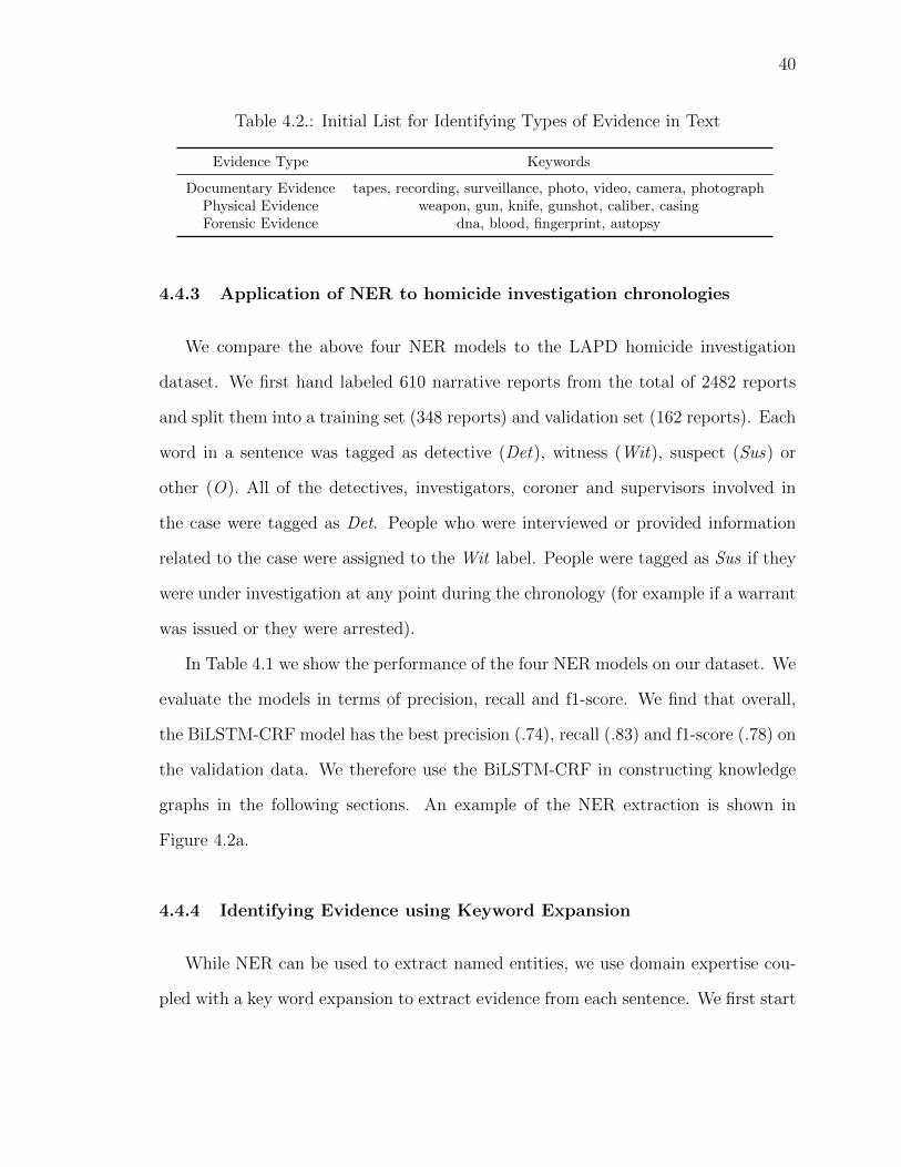
40

Table 4.2.: Initial List for Identifying Types of Evidence in Text

Evidence Type Keywords

Documentary Evidence tapes, recording, surveillance, photo, video, camera, photographPhysical Evidence weapon, gun, knife, gunshot, caliber, casingForensic Evidence dna, blood, fingerprint, autopsy

4.4.3 Application of NER to homicide investigation chronologies

We compare the above four NER models to the LAPD homicide investigation

dataset. We first hand labeled 610 narrative reports from the total of 2482 reports

and split them into a training set (348 reports) and validation set (162 reports). Each

word in a sentence was tagged as detective (Det), witness (Wit), suspect (Sus) or

other (O). All of the detectives, investigators, coroner and supervisors involved in

the case were tagged as Det. People who were interviewed or provided information

related to the case were assigned to the Wit label. People were tagged as Sus if they

were under investigation at any point during the chronology (for example if a warrant

was issued or they were arrested).

In Table 4.1 we show the performance of the four NER models on our dataset. We

evaluate the models in terms of precision, recall and f1-score. We find that overall,

the BiLSTM-CRF model has the best precision (.74), recall (.83) and f1-score (.78) on

the validation data. We therefore use the BiLSTM-CRF in constructing knowledge

graphs in the following sections. An example of the NER extraction is shown in

Figure 4.2a.

4.4.4 Identifying Evidence using Keyword Expansion

While NER can be used to extract named entities, we use domain expertise cou-

pled with a key word expansion to extract evidence from each sentence. We first start

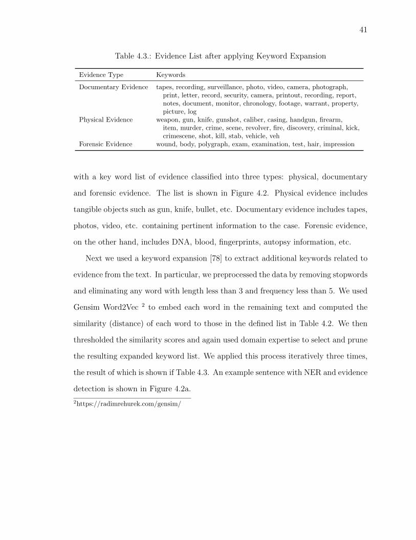
41

Table 4.3.: Evidence List after applying Keyword Expansion

Evidence Type Keywords

Documentary Evidence tapes, recording, surveillance, photo, video, camera, photograph,print, letter, record, security, camera, printout, recording, report,notes, document, monitor, chronology, footage, warrant, property,picture, log

Physical Evidence weapon, gun, knife, gunshot, caliber, casing, handgun, firearm,item, murder, crime, scene, revolver, fire, discovery, criminal, kick,crimescene, shot, kill, stab, vehicle, veh

Forensic Evidence wound, body, polygraph, exam, examination, test, hair, impression

with a key word list of evidence classified into three types: physical, documentary

and forensic evidence. The list is shown in Figure 4.2. Physical evidence includes

tangible objects such as gun, knife, bullet, etc. Documentary evidence includes tapes,

photos, video, etc. containing pertinent information to the case. Forensic evidence,

on the other hand, includes DNA, blood, fingerprints, autopsy information, etc.

Next we used a keyword expansion [78] to extract additional keywords related to

evidence from the text. In particular, we preprocessed the data by removing stopwords

and eliminating any word with length less than 3 and frequency less than 5. We used

Gensim Word2Vec 2 to embed each word in the remaining text and computed the

similarity (distance) of each word to those in the defined list in Table 4.2. We then

thresholded the similarity scores and again used domain expertise to select and prune

the resulting expanded keyword list. We applied this process iteratively three times,

the result of which is shown if Table 4.3. An example sentence with NER and evidence

detection is shown in Figure 4.2a.

2https://radimrehurek.com/gensim/

42

4.5 Building a Knowledge Graph of Homicide Investigation Chronologies

A knowledge graph (KG) is a representation of structured information in the form

of entities and relations (links) between them. Here we describe our approach to

constructing knowledge graphs of homicide investigation chronologies. We utilize an

end-to-end text to knowledge graph framework, t2kg, [79] to construct the knowledge

graph in four stages:

1. Entity Mapping

2. Coreference Resolution

3. Entity Extraction

4. Entity Disambiguation

During the first stage an entity is mapped to a uniform resource identifier (URI).

In the context of a homicide investigation, entity mapping can be viewed as identifying

law enforcement detectives, witnesses, suspects and evidences from text. In the next

stage, coreference resolution is the task of finding mentions in text that refer to the

same underlying entity. This is done in order to capture different expressions of

identical entities [80, 81]. For this purpose we use neuralcoref3 to resolve coreference

clusters. In the third stage we perform entity extraction, for which we considered the

following two approaches:

1. Triple Extraction Approach Subject-object-relation triples are extracted

using the Open Information Extraction technique implemented in the Stanford

CoreNLP library. In Figure 4.2b we show an example of a sub-graph created

from the paragraph in Figure 4.2a using the triple extraction approach. For

example, vehicle keys are provided to a witness leading to an edge between

vehicle and witness being added to the knowledge graph.

3https://spacy.io/universe/project/neuralcoref

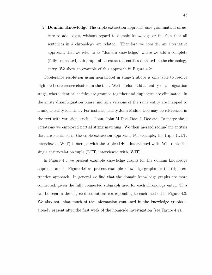
43

2. Domain Knowledge The triple extraction approach uses grammatical struc-

ture to add edges, without regard to domain knowledge or the fact that all

sentences in a chronology are related. Therefore we consider an alternative

approach, that we refer to as “domain knowledge,” where we add a complete

(fully-connected) sub-graph of all extracted entities detected in the chronology

entry. We show an example of this approach in Figure 4.2c.

Coreference resolution using neuralcoref in stage 2 above is only able to resolve

high level coreference clusters in the text. We therefore add an entity disambiguation

stage, where identical entities are grouped together and duplicates are eliminated. In

the entity disambiguation phase, multiple versions of the same entity are mapped to

a unique entity identifier. For instance, entity John Middle Doe may be referenced in

the text with variations such as John, John M Doe, Doe, J. Doe etc. To merge these

variations we employed partial string matching. We then merged redundant entities

that are identified in the triple extraction approach. For example, the triple (DET,

interviewed, WIT) is merged with the triple (DET, interviewed with, WIT) into the

single entity-relation tuple (DET, interviewed with, WIT).

In Figure 4.5 we present example knowledge graphs for the domain knowledge

approach and in Figure 4.6 we present example knowledge graphs for the triple ex-

traction approach. In general we find that the domain knowledge graphs are more

connected, given the fully connected subgraph used for each chronology entry. This

can be seen in the degree distributions corresponding to each method in Figure 4.3.

We also note that much of the information contained in the knowledge graphs is

already present after the first week of the homicide investigation (see Figure 4.4).

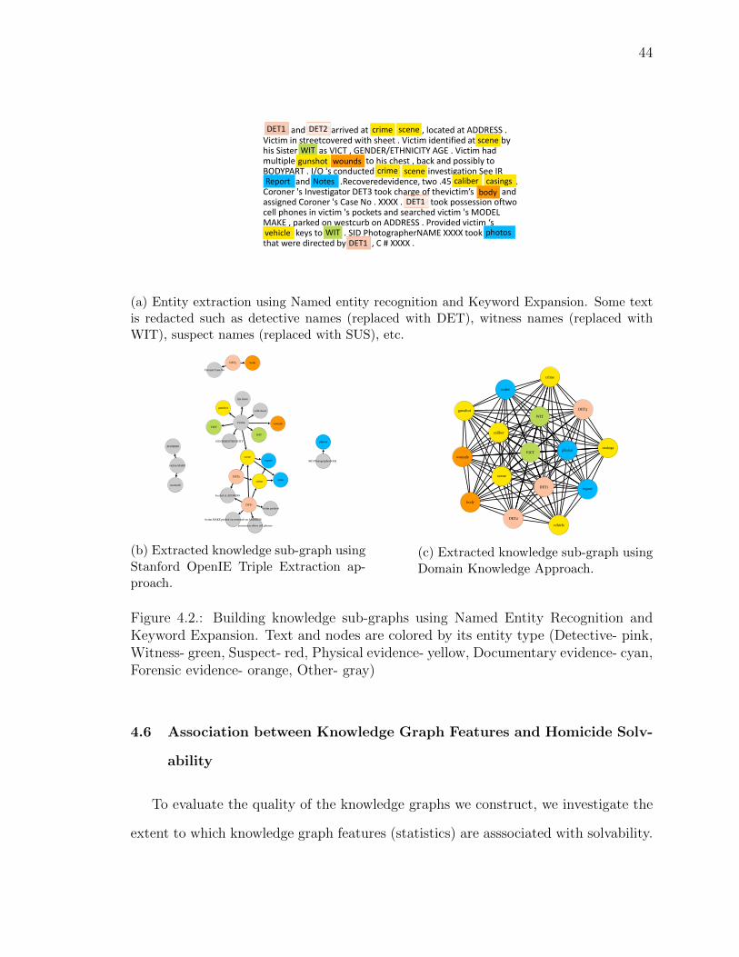
44

and arrived at , located at ADDRESS . Victim in streetcovered with sheet . Victim identified at by his Sister as VICT , GENDER/ETHNICITY AGE . Victim had multiple to his chest , back and possibly to BODYPART . I/O 's conducted investigation See IR

and .Recoveredevidence, two .45 . Coroner 's Investigator DET3 took charge of thevictim’s and assigned Coroner 's Case No . XXXX . took possession oftwocell phones in victim 's pockets and searched victim 's MODEL MAKE , parked on westcurb on ADDRESS . Provided victim ‘s

keys to . SID PhotographerNAME XXXX took that were directed by , C # XXXX .

DET1 DET2 crime scenescene

WITgunshot wounds

crime sceneReport Notes caliber casings

bodyDET1

vehicle WITDET1

photos

(a) Entity extraction using Named entity recognition and Keyword Expansion. Some textis redacted such as detective names (replaced with DET), witness names (replaced withWIT), suspect names (replaced with SUS), etc.

photos

with sheet

westcurb

victim pockets

DET2

ADDRESS

DET3

his chest

scene

located at ADDRESS

GENDER/ETHNICITY

WIT

Victim

crime

report

victim MAKE parked on westcurb on ADDRESS

SID PhotographerNAME

VICT

Coroner Case No

wounds

notes

gunshot

body

possession oftwo cell phones

DET1

victim MAKE

(b) Extracted knowledge sub-graph usingStanford OpenIE Triple Extraction ap-proach.

DET3

photosVICT

scene

caliber

wounds

casings

notes

vehicle

crime

gunshot

body

report

DET2

WIT

DET1

(c) Extracted knowledge sub-graph usingDomain Knowledge Approach.

Figure 4.2.: Building knowledge sub-graphs using Named Entity Recognition andKeyword Expansion. Text and nodes are colored by its entity type (Detective- pink,Witness- green, Suspect- red, Physical evidence- yellow, Documentary evidence- cyan,Forensic evidence- orange, Other- gray)

4.6 Association between Knowledge Graph Features and Homicide Solv-

ability

To evaluate the quality of the knowledge graphs we construct, we investigate the

extent to which knowledge graph features (statistics) are asssociated with solvability.

45

dk det dk no det te det te no det

2.5 5.0 7.5 10.0 2.5 5.0 7.5 10.0 2.5 5.0 7.5 10.0 2.5 5.0 7.5 10.00

20

40

60

80

0

25

50

75

5

10

3

6

9

degree

n

network dk det dk no det te det te no det

Figure 4.3.: Degree distributions of the 24 homicide investigation knowledge graphsof domain knowledge type (with and without detective nodes) and triple extractiontype (with and without detective nodes).

0.0 2.5 5.0 7.5 10.0 12.5 15.0 17.5 20.0Number of weeks

0

10

20

30

40

Num

ber o

f chr

onol

ogie

s

SolvedUnsolved

Figure 4.4.: Average number of chronology entries over first 20 weeks into the inves-tigation.

The methods we introduce here may be stepping stones towards AI-assisted homicide

investigation, where key elements of the graph may be identified as playing a role in

whether the case is ultimately solved (a suspect is charged for the crime). We are

cautious in avoiding the term prediction, given the small dataset size and our inability

to disentangle causality from correlation.

First, we create knowledge graphs for each of the 24 cases provided by the LAPD

using the triple extraction and domain knowledge approaches. After the creation of

the knowledge graphs, we compute network statistics for each KG, e.g., number of

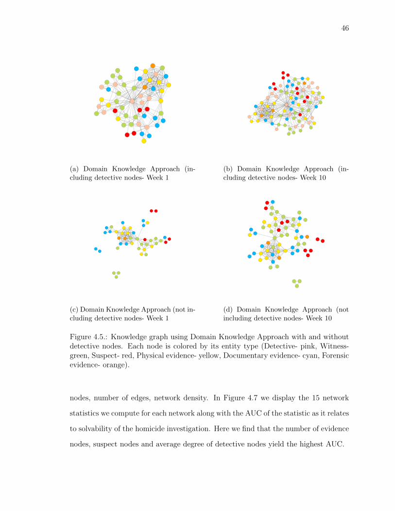
46

(a) Domain Knowledge Approach (in-cluding detective nodes- Week 1

(b) Domain Knowledge Approach (in-cluding detective nodes- Week 10

(c) Domain Knowledge Approach (not in-cluding detective nodes- Week 1

(d) Domain Knowledge Approach (notincluding detective nodes- Week 10

Figure 4.5.: Knowledge graph using Domain Knowledge Approach with and withoutdetective nodes. Each node is colored by its entity type (Detective- pink, Witness-green, Suspect- red, Physical evidence- yellow, Documentary evidence- cyan, Forensicevidence- orange).

nodes, number of edges, network density. In Figure 4.7 we display the 15 network

statistics we compute for each network along with the AUC of the statistic as it relates

to solvability of the homicide investigation. Here we find that the number of evidence

nodes, suspect nodes and average degree of detective nodes yield the highest AUC.

47

(a) Triple Extraction (including detectivenodes- Week 1

(b) Triple Extraction (including detectivenodes- Week 10

(c) Triple Extraction (after removing de-tective nodes- Week 1

(d) Triple Extraction (after removing de-tective nodes- Week 10

Figure 4.6.: Knowledge graph using Triple extraction approach with and withoutdetective nodes. Each node is colored by its entity type (Detective- pink, Witness-green, Suspect- red, Physical evidence- yellow, Documentary evidence- cyan, Forensicevidence- orange, Other- gray).

For each approach (domain knowledge and triple extraction), we consider networks

where detective nodes are included and networks where they are removed. While

detective node based features have a high AUC score, causality may be in the wrong

direction. On the one hand, an increase in the number of detective nodes may be due

48

●

●

●

●

●

●

●

●

●

●

●

●

●

●

●

●

●

●

●

●

●

●

●

●

●

●

●

●

●

●

●

●

●

●

●

●

●

●

●

●

●

●

●

●

●

●

●

●

●

●

●

●

●

●

●

●

●

●

●

●

DK Det DK No Det TE Det TE No Det

0.4 0.5 0.6 0.7 0.8 0.4 0.5 0.6 0.7 0.8 0.3 0.4 0.5 0.6 0.7 0.8 0.9 0.4 0.5 0.6 0.7 0.8density

avg degree detectivedet nodes

avg degree evidenceavg closeness centrality

avg node connspectral radius

avg clustering coefwit nodes

nodesavg degree witness

edgesevidence nodes

avg degree suspectsus nodes

densityavg closeness centrality

det nodesavg node conn

avg degree evidencespectral radius

avg clustering coefavg degree witness

wit nodesevidence nodes

nodesedges

sus nodesavg degree suspect

avg degree detective

avg clustering coefavg degree detective

det nodesavg node conn

avg closeness centralityavg degree witness

spectral radiuswit nodes

avg degree evidencedensityedgesnodes

avg degree suspectsus nodes

evidence nodes

avg degree evidenceavg closeness centrality

edgesavg clustering coef

densitydet nodes

avg degree witnessavg node connspectral radius

avg degree detectivenodes

avg degree suspectwit nodes

evidence nodessus nodes

AUC

Net

wor

k S

tatis

tic

Figure 4.7.: AUC and standard error for each network statistic in week 1 of theinvestigation.

to the case being solvable. On the other, cases with more dedicated resources may

be more likely to be solved. We show results for both types of networks.

We next evaluate a simple generalized linear model (GLM) with binary response

for determining solvability:

log(p(y = 1)/(1− p(y = 1)) = c0 + c1s+ c2e+ c3s · e (4.1)

where s is the number of suspect nodes, e is the number of evidence nodes, and y

indicates whether the homicide is solved. The features were selected based on their

individual AUC scores in Figure 4.7 and limited to the top-two (averaged across

network types) to prevent over-fitting.

Due to the small dataset size we use leave-one-out cross validation (LOOCV). In

Figure 4.8 we show the AUC scores of the GLM model for each network type (domain

knowledge vs. tripe extraction, with and without detective nodes) constructed using

data up to a given week past the start of the investigation. Here we generally find

that the domain knowledge approach outperforms the triple extraction approach. We

also do not find much improvement in the association between the model scores and

solvability past 1-3 weeks in the investigation. In the case of the triple extraction

networks without detective nodes, we find that the GLM model yields AUC scores at

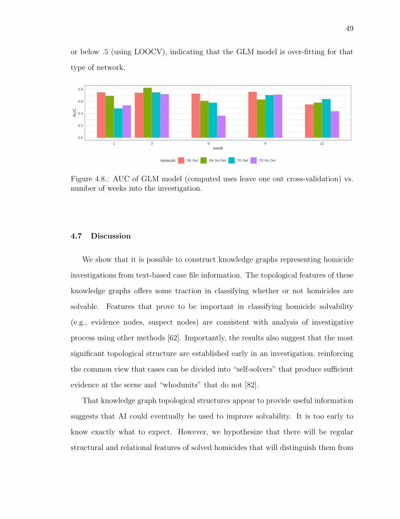
49

or below .5 (using LOOCV), indicating that the GLM model is over-fitting for that

type of network.

0.0

0.2

0.4

0.6

0.8

1 3 6 9 12week

AU

C

network DK Det DK No Det TE Det TE No Det

Figure 4.8.: AUC of GLM model (computed uses leave one out cross-validation) vs.number of weeks into the investigation.

4.7 Discussion

We show that it is possible to construct knowledge graphs representing homicide

investigations from text-based case file information. The topological features of these

knowledge graphs offers some traction in classifying whether or not homicides are

solvable. Features that prove to be important in classifying homicide solvability

(e.g., evidence nodes, suspect nodes) are consistent with analysis of investigative

process using other methods [62]. Importantly, the results also suggest that the most

significant topological structure are established early in an investigation, reinforcing

the common view that cases can be divided into “self-solvers” that produce sufficient

evidence at the scene and “whodunits” that do not [82].

That knowledge graph topological structures appear to provide useful information

suggests that AI could eventually be used to improve solvability. It is too early to

know exactly what to expect. However, we hypothesize that there will be regular

structural and relational features of solved homicides that will distinguish them from

50

unsolved ones. When comparing graphs, we may be able to identify gaps or holes in

graphical structures that, if closed, could improve the chances of a case being solved.

To the extent that such graph-based insights go beyond what common investigative

practice would yield, AI-assisted homicide investigation may be valuable.

A common expressed view is that solving homicides helps build community trust

in police, while failure to do so erodes that trust and creates a sense of impunity

among offenders [58, 59]. If AI can help improve homicide solvability, then it can

also be seen to contribute to building community trust. However, the question is

not simply whether such methods augment the process of homicide investigation.

Rather, since homicide investigations must adhere to the policy requirements of the

organization and the procedural requirements of the law, so must AI used within those

investigations. For example, if we consider a hypothetical knowledge graph-based

recommender system that suggests investigative steps, then those recommendations

cannot violate policy or the law.

AI-assisted homicide investigation would also need to be evaluated in terms of

fairness. The evidence is mixed on whether homicide clearance rates are mediated by

race and gender [56, 59, 62, 83], though many expect that clearances rates are lower

when the victim is a person of color [58]. In any case, AI should not introduce or

amplify any clearance rate imbalances. We should also consider the possibility that

AI-assisted investigation might ease clearance rate imbalances. Such imbalances may

originate with the event itself if, for instance, so-called “whodunit” cases arise more

often in association with certain demographic characteristics [84]. They might also

appear if there is “victim devaluing” based on demographic characteristics [58, 59].

Identifying such biases in investigative knowledge graphs is a necessary and important

step towards correcting for them.

51

Finally, we must also be aware of the potential for the miscarriage of justice.

Recent evidence suggests that wrongful convictions may occur in < 5% of capital cases

such as murder [85]. That wrongful convictions may also differ by race [86], demands

that the contributing factors be taken into consideration in AI-assisted homicide

investigations. While careful adherence to rules of evidence and procedure may offer

some protection, it does not provide a guarantee. Wrongful convictions can sometimes

be linked back to false witness statements, forensic error, or police misconduct [87].

Eventually, whether there are recognizable differences between knowledge graphs that

include corrupted information and those that do not needs to be investigated.

Ultimately, considerations of fairness, accountability, and transparency need to be

central to the development of machine learning methods for homicide investigations.

52

5. SUMMARY

In this work, we proposed machine learning methodologies to address social harm

issues. In particular, we evaluated crime topic models, investigated transitions into

drug addiction and analyzed homicide investigation chronologies using knowledge

graph based framework.

The crime topic modeling exhibit a more nuanced model of crime incidents which

entails the massive loss of information resulting from FBI Uniform Crime Reporting

[8]. We suggested two performance metrics for the evaluation of crime topic models

and demonstrated that choice of topic model has important implications for detecting

crime hotspots. We showed that it is possible to achieve more coherent topics that

simultaneously concentrate to a higher degree in space, allowing for more targeted

police intervention given limited resources.

Another problem we explored was the transition from recreational substance use

to substance abuse using voluntary generated introspective text in Reddit forums.

We proposed a prediction model that provides both the classification and likelihood

over time indicating a propensity of a user to become a drug addiction victim. Our

study indicates user’s transition into drug addiction can be predicted by the keywords

and linguistic features of the his post and most frequent drug names in his post.

Furthermore, we proposed a knowledge graph based framework for homicide in-

vestigation chronologies. Homicide investigations chronology tracks the evolution of

an investigation, including when and how persons involved and items of evidence

became part of a case. We performed named entity recognition to determine de-

tectives, witness and suspects from chronology entries and also extracted different

53

evidence types using keyword expansion. We further linked entities and evidence to

construct a knowledge graph and analyzed the association between network statistics

of knowledge graph and homicide solvability.

54

6. PUBLICATIONS

In this section, we provide the list of our publications:

1. Pandey, Ritika and Mohler, George ”Evaluation of crime topic models: topic

coherence vs spatial crime concentration,” 2018 IEEE International Conference

on Intelligence and Security Informatics (ISI), Miami, FL, 2018, pp. 76-78, doi:

10.1109/ISI.2018.8587384.

2. John Lu, Sumati Sridhar, Ritika Pandey, Mohammad Al Hasan, and Geo-

rege Mohler. 2019. Investigate Transitions into Drug Addiction through Text

Mining of Reddit Data. In Proceedings of the 25th ACM SIGKDD Interna-

tional Conference on Knowledge Discovery Data Mining (KDD ’19). As-

sociation for Computing Machinery, New York, NY, USA, 2367–2375. doi:

https://doi.org/10.1145/3292500.3330737.

REFERENCES

55

REFERENCES

[1] Paddy Hillyard and Steve Tombs. From ‘crime’ to social harm? Crime, Law andSocial Change, 48:9–25, 01 2007.

[2] Paddy Hillyard and Steve Tombs. Beyond Criminology: Taking Harm Seriously.Pluto Press, 2004.

[3] Danny Dorling, Dave Gordon, Paddy Hillyard, Christina Pantazis, Simon Pem-berton, and Steve Tombs. Criminal Obsessions: Why Harm Matters More ThanCrime (2nd ed.). Harm and Society. Centre for Crime and Justice Studies, Lon-don, 2008.

[4] Simon Pemberton. Social harm future(s): Exploring the potential of the socialharm approach. Crime, Law and Social Change, 48:27–41, 01 2007.

[5] S. V. Nath. Crime Pattern Detection Using Data Mining. In 2006IEEE/WIC/ACM International Conference on Web Intelligence and IntelligentAgent Technology Workshops, pages 41–44, 2006.

[6] H. Chen, W. Chung, J. J. Xu, G. Wang, Y. Qin, and M. Chau. Crime datamining: a general framework and some examples. Computer, 37(4):50–56, 2004.

[7] Mohammad Keyvanpour, Mostafa Javideh, and Mohammadreza Ebrahimi. De-tecting and investigating crime by means of data mining: A general crime match-ing framework. Procedia CS, 3:872–880, 12 2011.

[8] Da Kuang, P Jeffrey Brantingham, and Andrea L Bertozzi. Crime topic model-ing. Crime Science, 6(1):12, 2017.

[9] Munmun De Choudhury, Emre Kiciman, Mark Dredze, Glen Coppersmith, andMrinal Kumar. Discovering Shifts to Suicidal Ideation from Mental Health Con-tent in Social Media. In Proceedings of the 2016 CHI Conference on HumanFactors in Computing Systems, CHI ’16, page 2098–2110, New York, NY, USA,2016. Association for Computing Machinery.

[10] George Mohler, Jeremy Carter, and Rajeev Raje. Improving social harm indiceswith a modulated hawkes process. International Journal of Forecasting, 34(3):431– 439, 2018.

[11] R. Eshleman, D. Jha, and R. Singh. Identifying individuals amenable to drugrecovery interventions through computational analysis of addiction content insocial media. In 2017 IEEE International Conference on Bioinformatics andBiomedicine (BIBM), pages 849–854, 2017.

56

[12] Benjamin Fischman. Data Driven Support for Substance Addiction RecoveryCommunities. In Extended Abstracts of the 2018 CHI Conference on HumanFactors in Computing Systems, CHI EA ’18, page 1–6, New York, NY, USA,2018. Association for Computing Machinery.

[13] Diana MacLean, Sonal Gupta, Anna Lembke, Christopher Manning, and JeffreyHeer. Forum77: An Analysis of an Online Health Forum Dedicated to AddictionRecovery. In Proceedings of the 18th ACM Conference on Computer SupportedCooperative Work Social Computing, CSCW ’15, page 1511–1526, New York,NY, USA, 2015. Association for Computing Machinery.

[14] Kadhim Al-Janabi and Hayder Fatlawi. Crime Data Analysis Using Data MiningTechniques To Improve Crimes Prevention Procedures. 01 2010.

[15] Shyam Varan. Crime Pattern Detection Using Data Mining. pages 41 – 44, 012007.

[16] Saurabh Pandey, Nahida Chowdhury, Milan Patil, Rajeev Raje, George Mohler,and Jeremy Carter. CDASH: Community Data Analytics for Social Harm Pre-vention. 08 2018.

[17] David Newman, Jey Han Lau, Karl Grieser, and Timothy Baldwin. AutomaticEvaluation of Topic Coherence. In Human Language Technologies: The 2010Annual Conference of the North American Chapter of the Association for Com-putational Linguistics, HLT ’10, pages 100–108, Stroudsburg, PA, USA, 2010.Association for Computational Linguistics.

[18] Patricia L. Brantingham and Paul J. Brantingham. Nodes, paths and edges:Considerations on the complexity of crime and the physical environment. Journalof Environmental Psychology, 13(1):3 – 28, 1993.

[19] David Weisburd. The law of crime concentration and the criminology of place.Criminology, 53, 05 2015.

[20] Anthony A Braga, Andrew V Papachristos, and David M Hureau. The effects ofhot spots policing on crime: An updated systematic review and meta-analysis.Justice quarterly, 31(4):633–663, 2014.

[21] David M Blei, Andrew Y Ng, and Michael I Jordan. Latent dirichlet allocation.Journal of machine Learning research, 3(Jan):993–1022, 2003.

[22] Nicolas Gillis. The why and how of nonnegative matrix factorization. Regular-ization, Optimization, Kernels, and Support Vector Machines, 12(257), 2014.

[23] Wei Xu, Xin Liu, and Yihong Gong. Document Clustering Based On Non-negative Matrix Factorization. In SIGIR Forum (ACM Special Interest Groupon Information Retrieval), pages 267–273, 01 2003.

[24] David Mimno, Hanna M. Wallach, Edmund Talley, Miriam Leenders, and An-drew McCallum. Optimizing Semantic Coherence in Topic Models. In Proceed-ings of the Conference on Empirical Methods in Natural Language Processing,EMNLP ’11, pages 262–272, Stroudsburg, PA, USA, 2011. Association for Com-putational Linguistics.

57

[25] Wim Bernasco and Wouter Steenbeek. More Places than Crimes: Implicationsfor Evaluating the Law of Crime Concentration at Place. Journal of QuantitativeCriminology, 33(3):451–467, Sep 2017.

[26] John E Eck, YongJei Lee, O SooHyun, and Natalie Martinez. Compared towhat? Estimating the relative concentration of crime at places using systematicand other reviews. Crime Science, 6(1):8, 2017.

[27] Martin Rajman and Romaric Besancon. Text Mining - Knowledge extractionfrom unstructured textual data. In Alfredo Rizzi, Maurizio Vichi, and Hans-Hermann Bock, editors, Advances in Data Science and Classification, pages 473–480, Berlin, Heidelberg, 1998. Springer Berlin Heidelberg.

[28] Juan Ramos et al. Using tf-idf to determine word relevance in document queries.In Proceedings of the first instructional conference on machine learning, volume242, pages 133–142, 2003.

[29] George Mohler and P Jeffrey Brantingham. Privacy preserving, crowd sourcedcrime Hawkes processes. In Social Sensing (SocialSens), 2018 InternationalWorkshop on, pages 14–19. IEEE, 2018.

[30] Richard J. Bonnie, Morgan A. Ford, and Jonathan K. Phillips. Pain Managementand the Opioid Epidemic: Balancing Societal and Individual Benefits and Risksof Prescription Opioid Use. The National Academies Press, 2017.

[31] Jonathan Penm, Neil J. MacKinnon, Jill M. Boone, Antonio Ciaccia, CameronMcNamee, and Erin L. Winstanley. Strategies and policies to address the opioidepidemic: A case study of Ohio. Journal of the American Pharmacists Associa-tion, 57(2, Supplement):S148 – S153, 2017.

[32] Puja Seth, Lawrence Scholl, Rose Rudd, and Sarah Bacon. Overdose deathsinvolving opioids, cocaine, and psychostimulants — United States, 2015–2016.American Journal of Transplantation, 18:1556–1568, 06 2018.

[33] Self-Help/Recovery Support Group.

[34] Samantha P Wallace Kathlene Tracy. Benefits of peer support groups in thetreatment of addiction. Substance Abuse and Rehabilitation, 7.

[35] Jason B. Luoma, Barbara S. Kohlenberg, Steven C. Hayes, Kara Bunting, andAlyssa K. Rye. Reducing self-stigma in substance abuse through acceptanceand commitment therapy: Model, manual development, and pilot outcomes.Addiction Research & Theory, 16(2):149–165, 2008.

[36] Magdalena Berger, Todd H. Wagner, and Laurence C. Baker. Internet use andstigmatized illness. Social Science and Medicine, 61(8):1821 – 1827, 2005.

[37] Kim Jung Sunny, Marsch A. Lisa, Hancock T. Jeffrey, and Das K. Amarendra.Scaling Up Research on Drug Abuse and Addiction Through Social Media BigData. J Med Internet Res, 19(10):e353, Oct 2017.

[38] Michael J. Paul and Mark Dredze. Experimenting with Drugs (and Topic Mod-els): Multi-Dimensional Exploration of Recreational Drug Discussions. In Proc.of AAAI, 2012.

58

[39] Abeed Sarker, Karen O’Connor, Rachel Ginn, Matthew Scotch, Karen Smith,Dan Malone, and Graciela Gonzalez. Social Media Mining for Toxicovigilance:Automatic Monitoring of Prescription Medication Abuse from Twitter. DrugSafety, 39(3):231–240, Mar 2016.

[40] Wilson M. Compton, Christopher M. Jones, and Grant T. Baldwin. Relationshipbetween Nonmedical Prescription-Opioid Use and Heroin Use. New EnglandJournal of Medicine, 374(2):154–163, 2016.

[41] Andrew Kolodny, David T. Courtwright, Catherine S. Hwang, Peter Kreiner,John L. Eadie, Thomas W. Clark, and G. Caleb Alexander. The PrescriptionOpioid and Heroin Crisis: A Public Health Approach to an Epidemic of Addic-tion. Annual Review of Public Health, 36(1):559–574, 2015.

[42] Mark Edmund Rose. Are Prescription Opioids Driving the Opioid Crisis? As-sumptions vs Facts. Pain Medicine, 19(4):793–807, 2018.

[43] Ahn, Woo-Young, Vassileva, and Jasmin. Machine-learning identifies substance-specific behavioral markers for opiate and stimulant dependence. Drug and Al-cohol Dependence, 161, 2016/04/01.

[44] A. Hutchinson. Reddit Now Has as Many Users as Twitter, and Far HigherEngagement Rates.

[45] Gensim: Doc2Vec Paragraph Embeddings.

[46] Quoc Le and Tomas Mikolov. Distributed Representations of Sentences andDocuments. In Proceedings of the 31st International Conference on InternationalConference on Machine Learning - Volume 32, ICML’14, pages II–1188–II–1196.JMLR.org, 2014.

[47] Dragomir R. Radev, Hongyan Jing, Malgorzata Stys, and Daniel Tam. Centroid-based Summarization of Multiple Documents. Inf. Process. Manage., 40(6):919–938, November 2004.

[48] Kaustubh Mani, Ishan Verma, and Lipika Dey. Multi-Document Summarizationusing Distributed Bag-of-Words Model. CoRR, abs/1710.02745, 2017.

[49] James W. Pennebaker. The secret life of pronouns: what our words say aboutus. Bloomsbury Press, 2013.

[50] James W. Pennebaker, Matthias R. Mehl, and Kate G. Niederhoffer. Psycholog-ical Aspects of Natural Language Use: Our Words, Our Selves. Annual Reviewof Psychology, 54(1):547–577, 2003.

[51] M. R. Gossop and S. B. Eysenck. A further investigation into the personality ofdrug addicts in treatment. Addiction, 75(3):305–311, 1980.

[52] Harald Steck, Balaji Krishnapuram, Cary Dehing-oberije, Philippe Lambin, andVikas C Raykar. On Ranking in Survival Analysis: Bounds on the ConcordanceIndex. In Advances in Neural Information Processing Systems 20, pages 1209–1216. Curran Associates, Inc., 2008.

[53] David Nutt, Leslie A King, William Saulsbury, and Colin Blakemore. Develop-ment of a rational scale to assess the harm of drugs of potential misuse. TheLancet, 369(9566):1047 – 1053, 2007.

59

[54] Aaron L. Sarvet, Melanie M. Wall, David S. Fink, Emily Greene, Aline Le,Anne E. Boustead, Rosalie Liccardo Pacula, Katherine M. Keyes, MagdalenaCerda, Sandro Galea, and Deborah S. Hasin. Medical marijuana laws and adoles-cent marijuana use in the United States: a systematic review and meta-analysis.Addiction, 113(6):1003–1016.

[55] FBI. Crime in the United States. 2017.

[56] Charles Wellford and James Cronin. Clearing up homicide clearance rates. Na-tional Institute of Justice Journal, 243:1–7, 2000.

[57] Aki Roberts. Predictors of homicide clearance by arrest: An event history anal-ysis of NIBRS incidents. Homicide Studies, 11(2):82–93, 2007.

[58] Jill Leovy. Ghettoside: A True Story of Murder in America. Spiegel Grau, NewYork, 2015.

[59] Paige E. Vaughn. The effects of devaluation and solvability on crime clear-ance, journal = Journal of Criminal Justice, volume = 68, pages = 101657,issn = 0047-2352, doi = https://doi.org/10.1016/j.jcrimjus.2020.101657, url =http://www.sciencedirect.com/science/article/pii/S0047235219303848, year =2020, type = Journal Article.

[60] Anthony A. Braga and Desiree Dusseault. Can Homicide Detectives ImproveHomicide Clearance Rates? Crime Delinquency, 64(3):283–315, 2018.

[61] Fiona Brookman and Martin Innes. The problem of success: What is a‘good’homicide investigation? Policing and society, 23(3):292–310, 2013.

[62] Wendy C Regoeczi. Solving homicides: Understanding trends and patterns inpolice clearances of lethal violence, pages 121–138. Emerald Publishing Limited,2018.

[63] L. E. Cohen and M. Felson. Social change and crime rate trends: A routineactivity approach. Am Sociol Rev, 44, 1979.

[64] Ogerta Elezaj, Sule Yildirim Yayilgan, Edlira Kalemi, Linda Wendelberg, Mo-hamed Abomhara, and Javed Ahmed. Towards Designing a Knowledge Graph-Based Framework for Investigating and Preventing Crime on Online Social Net-works. E-Democracy – Safeguarding Democracy and Human Rights in the DigitalAge, pages 181–195. Springer International Publishing, 2020.

[65] Tian Xia and Yijun Gu. Building Terrorist Knowledge Graph from Global Ter-rorism Database and Wikipedia. In 2019 IEEE International Conference onIntelligence and Security Informatics (ISI), pages 194–196. IEEE.

[66] Police Foundation and United States of America. Homicide Investigation CaseFile Profile: The Los Angeles Police Department Murder Book. 2018.

[67] Vikas Yadav and Steven Bethard. A Survey on Recent Advances in Named EntityRecognition from Deep Learning models. In Proceedings of the 27th InternationalConference on Computational Linguistics, pages 2145–2158, 2018.

[68] Matthew Honnibal and Ines Montani. spaCy 2: Natural language understandingwith Bloom embeddings, convolutional neural networks and incremental parsing.Preprint., 2017.

60

[69] Mark Neumann, Daniel King, Iz Beltagy, and Waleed Ammar. ScispaCy: Fastand Robust Models for Biomedical Natural Language Processing. In Proceedingsof the 18th BioNLP Workshop and Shared Task, pages 319–327, 2019.

[70] Joan Serra and Alexandros Karatzoglou. Getting deep recommenders fit: Bloomembeddings for sparse binary input/output networks. In Proceedings of theEleventh ACM Conference on Recommender Systems, pages 279–287, 2017.

[71] Zhiheng Huang, Wei Xu, and Kai Yu. Bidirectional LSTM-CRF Models forSequence Tagging. CoRR, abs/1508.01991, 2015.

[72] Jeffrey Pennington, Richard Socher, and Christopher D Manning. Glove: Globalvectors for word representation. In Proceedings of the 2014 conference on empir-ical methods in natural language processing (EMNLP), pages 1532–1543, 2014.

[73] Guillaume Genthial. Sequence Tagging with tensorflow, 2018.

[74] Guillaume Lample, Miguel Ballesteros, Sandeep Subramanian, KazuyaKawakami, and Chris Dyer. Neural Architectures for Named Entity Recogni-tion. In Proceedings of NAACL-HLT, pages 260–270, 2016.

[75] Xuezhe Ma and Eduard Hovy. End-to-end Sequence Labeling via Bi-directionalLSTM-CNNs-CRF. In Proceedings of the 54th Annual Meeting of the Associationfor Computational Linguistics (Volume 1: Long Papers), pages 1064–1074, 2016.

[76] Jason P.C. Chiu and Eric Nichols. Named Entity Recognition with BidirectionalLSTM-CNNs. Transactions of the Association for Computational Linguistics,4:357–370, 2016.

[77] Cıcero Nogueira Dos Santos and Bianca Zadrozny. Learning Character-LevelRepresentations for Part-of-Speech Tagging. In Proceedings of the 31st Interna-tional Conference on International Conference on Machine Learning - Volume32, ICML’14, page II–1818–II–1826. JMLR.org, 2014.

[78] Cody Buntain, Erin McGrath, and Brandon Behlendorf. Sampling social me-dia: Supporting information retrieval from microblog data resellers with text,network, and spatial analysis. In Proceedings of the 51st Hawaii InternationalConference on System Sciences, 2018.

[79] Natthawut Kertkeidkachorn and Ryutaro Ichise. T2KG: An end-to-end sys-tem for creating knowledge graph from unstructured text. In Workshops at theThirty-First AAAI Conference on Artificial Intelligence, 2017.

[80] Kevin Clark and Christopher D Manning. Deep Reinforcement Learning forMention-Ranking Coreference Models. In Proceedings of the 2016 Conference onEmpirical Methods in Natural Language Processing, pages 2256–2262, 2016.

[81] Kevin Clark and Christopher D Manning. Improving Coreference Resolution byLearning Entity-Level Distributed Representations. In Proceedings of the 54thAnnual Meeting of the Association for Computational Linguistics (Volume 1:Long Papers), pages 643–653, 2016.

[82] Marc Riedel and John Jarvis. The decline of arrest clearances for criminal homi-cide: Causes, correlates, and third parties. Criminal Justice Policy Review,9(3-4):279–306, 1999.

61

[83] Catherine Lee. The value of life in death: Multiple regression and event historyanalyses of homicide clearance in Los Angeles County, journal = Journal ofCriminal Justice. 33(6):527–534, 2005.

[84] Cheryl L. Maxson, Margaret A. Gordon, and Malcolm W. Klein. Differencesbetween gang and nongang homicides. Criminology, 23(2):209–222, 1985.

[85] Charles E. Loeffler, Jordan Hyatt, and Greg Ridgeway. Measuring Self-ReportedWrongful Convictions Among Prisoners. Journal of Quantitative Criminology,2018.

[86] Samuel R Gross, Kristen Jacoby, Daniel J Matheson, and Nicholas Montgomery.Exonerations in the United States 1989 through 2003. J. Crim. l. & CrimiNology,95:523, 2004.

[87] Jon Gould and Richard Leo. One Hundred Years Later: Wrongful ConvictionsAfter a Century of Research. Journal of Criminal Law and Criminology, 100, 062010.