TEXT CLASSIFICATION USING MACHINE LEARNING

_______________

A Thesis

Presented to the

Faculty of

San Diego State University

_______________

In Partial Fulfillment

of the Requirements for the Degree

Master of Science

in

Computer Science

_______________

by

Vinay Kumar Polisetty

Summer 2012

iii

Copyright © 2012

by

Vinay Kumar Polisetty

All Rights Reserved

iv

DEDICATION

Firstly, I would like to dedicate my work to my dad Ramesh and mom Sunita whose

moral support has constantly made me believe in myself, to achieve my dreams with all hard

work and dedication. Secondly, I would like to dedicate this to my friends and well-wishers

for being there whenever I needed them for a valuable input.

v

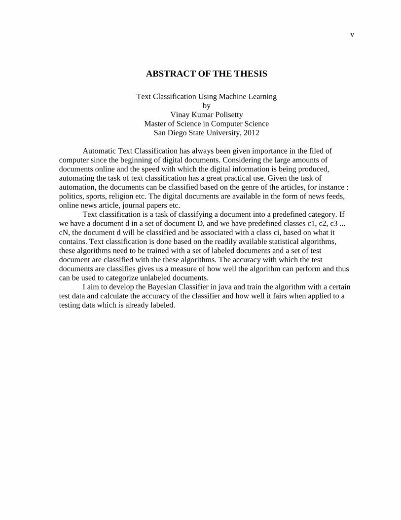
ABSTRACT OF THE THESIS

Text Classification Using Machine Learning by

Vinay Kumar Polisetty Master of Science in Computer Science

San Diego State University, 2012

Automatic Text Classification has always been given importance in the filed of computer since the beginning of digital documents. Considering the large amounts of documents online and the speed with which the digital information is being produced, automating the task of text classification has a great practical use. Given the task of automation, the documents can be classified based on the genre of the articles, for instance : politics, sports, religion etc. The digital documents are available in the form of news feeds, online news article, journal papers etc.

Text classification is a task of classifying a document into a predefined category. If we have a document d in a set of document D, and we have predefined classes c1, c2, c3 ... cN, the document d will be classified and be associated with a class ci, based on what it contains. Text classification is done based on the readily available statistical algorithms, these algorithms need to be trained with a set of labeled documents and a set of test document are classified with the these algorithms. The accuracy with which the test documents are classifies gives us a measure of how well the algorithm can perform and thus can be used to categorize unlabeled documents.

I aim to develop the Bayesian Classifier in java and train the algorithm with a certain test data and calculate the accuracy of the classifier and how well it fairs when applied to a testing data which is already labeled.

vi

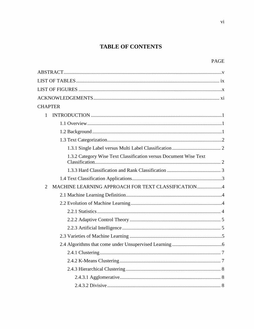
TABLE OF CONTENTS

PAGE

ABSTRACT ...............................................................................................................................v

LIST OF TABLES ................................................................................................................... ix

LIST OF FIGURES ...................................................................................................................x

ACKNOWLEDGEMENTS ..................................................................................................... xi

CHAPTER

1 INTRODUCTION .........................................................................................................1 1.1 Overview ............................................................................................................1 1.2 Background ........................................................................................................1 1.3 Text Categorization ............................................................................................2

1.3.1 Single Label versus Multi Label Classification ....................................... 2 1.3.2 Category Wise Text Classification versus Document Wise Text Classification..................................................................................................... 2 1.3.3 Hard Classification and Rank Classification ........................................... 3

1.4 Text Classification Applications ........................................................................3 2 MACHINE LEARNING APPROACH FOR TEXT CLASSIFICATION ....................4

2.1 Machine Learning Definition .............................................................................4 2.2 Evolution of Machine Learning .........................................................................4

2.2.1 Statistics ................................................................................................... 4 2.2.2 Adaptive Control Theory ......................................................................... 5 2.2.3 Artificial Intelligence ............................................................................... 5

2.3 Varieties of Machine Learning ..........................................................................5 2.4 Algorithms that come under Unsupervised Learning ........................................6

2.4.1 Clustering ................................................................................................. 7 2.4.2 K-Means Clustering ................................................................................. 7 2.4.3 Hierarchical Clustering ............................................................................ 8

2.4.3.1 Agglomerative................................................................................. 8 2.4.3.2 Divisive ........................................................................................... 8

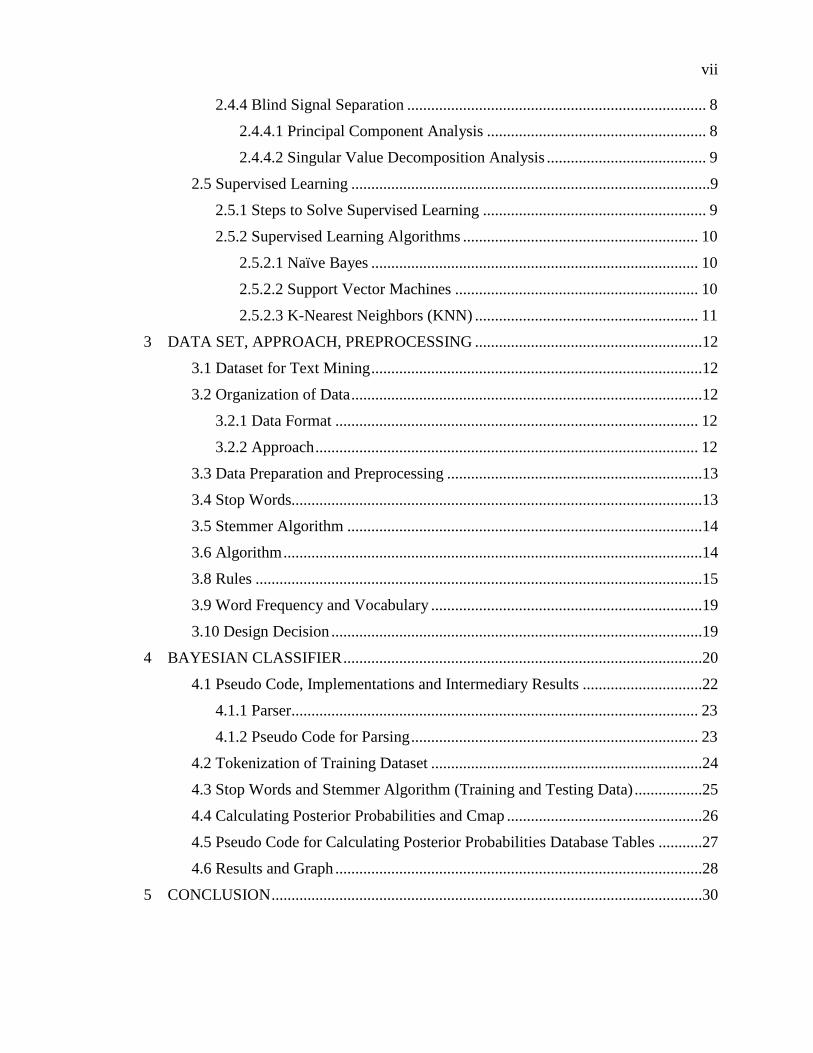
vii

2.4.4 Blind Signal Separation ........................................................................... 8 2.4.4.1 Principal Component Analysis ....................................................... 8 2.4.4.2 Singular Value Decomposition Analysis ........................................ 9

2.5 Supervised Learning ..........................................................................................9 2.5.1 Steps to Solve Supervised Learning ........................................................ 9 2.5.2 Supervised Learning Algorithms ........................................................... 10

2.5.2.1 Naïve Bayes .................................................................................. 10 2.5.2.2 Support Vector Machines ............................................................. 10 2.5.2.3 K-Nearest Neighbors (KNN) ........................................................ 11

3 DATA SET, APPROACH, PREPROCESSING .........................................................12 3.1 Dataset for Text Mining ...................................................................................12 3.2 Organization of Data ........................................................................................12

3.2.1 Data Format ........................................................................................... 12 3.2.2 Approach ................................................................................................ 12

3.3 Data Preparation and Preprocessing ................................................................13 3.4 Stop Words.......................................................................................................13 3.5 Stemmer Algorithm .........................................................................................14 3.6 Algorithm .........................................................................................................14 3.8 Rules ................................................................................................................15 3.9 Word Frequency and Vocabulary ....................................................................19 3.10 Design Decision .............................................................................................19

4 BAYESIAN CLASSIFIER ..........................................................................................20 4.1 Pseudo Code, Implementations and Intermediary Results ..............................22

4.1.1 Parser...................................................................................................... 23 4.1.2 Pseudo Code for Parsing ........................................................................ 23

4.2 Tokenization of Training Dataset ....................................................................24 4.3 Stop Words and Stemmer Algorithm (Training and Testing Data) .................25 4.4 Calculating Posterior Probabilities and Cmap .................................................26 4.5 Pseudo Code for Calculating Posterior Probabilities Database Tables ...........27 4.6 Results and Graph ............................................................................................28

5 CONCLUSION ............................................................................................................30

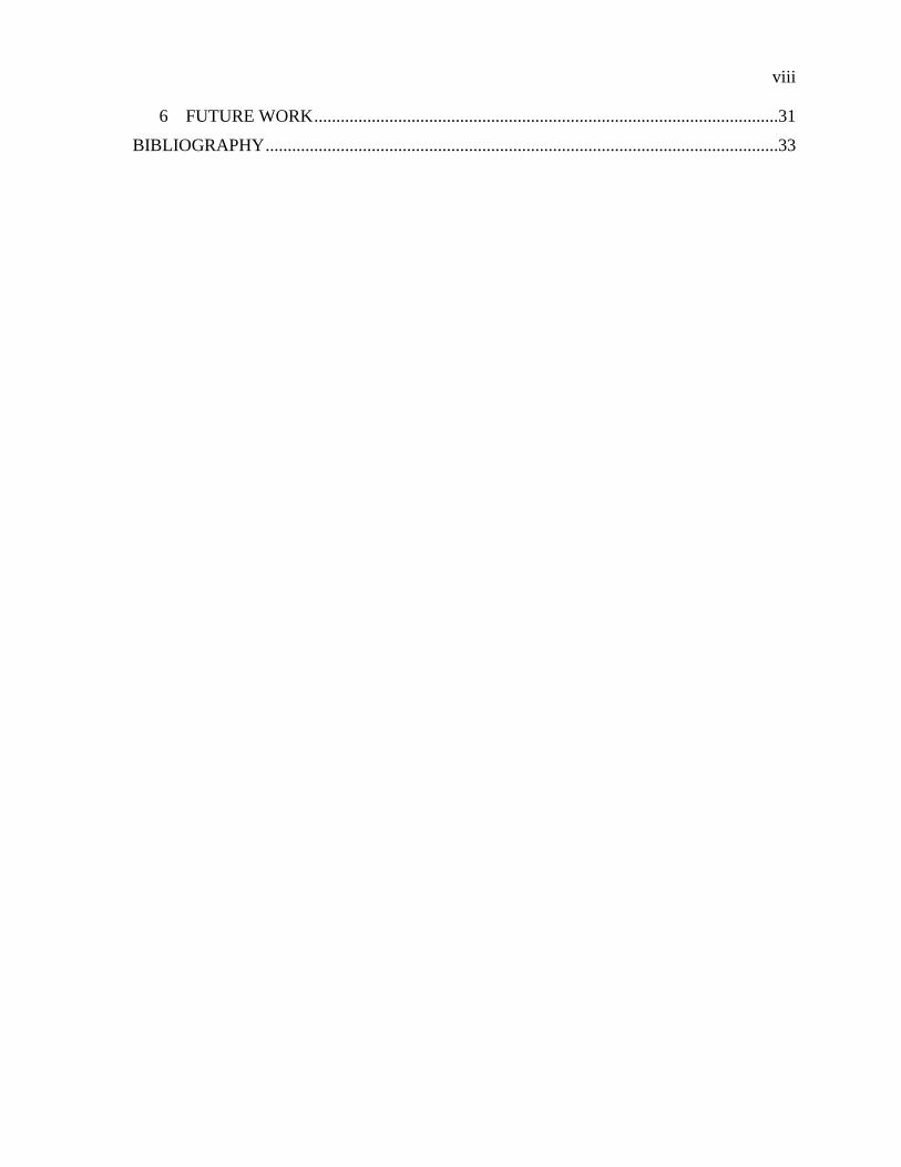
viii

6 FUTURE WORK .........................................................................................................31 BIBLIOGRAPHY ....................................................................................................................33

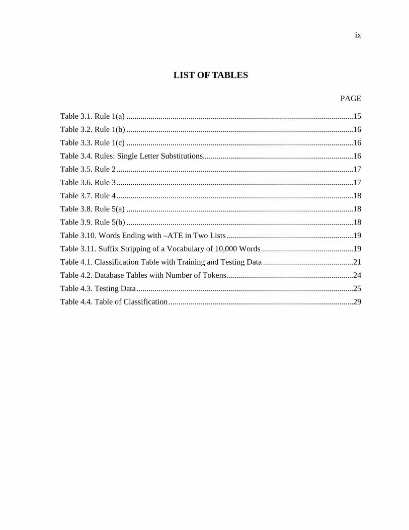
ix

LIST OF TABLES

PAGE

Table 3.1. Rule 1(a) .................................................................................................................15 Table 3.2. Rule 1(b) .................................................................................................................16 Table 3.3. Rule 1(c) .................................................................................................................16 Table 3.4. Rules: Single Letter Substitutions...........................................................................16 Table 3.5. Rule 2 ......................................................................................................................17 Table 3.6. Rule 3 ......................................................................................................................17 Table 3.7. Rule 4 ......................................................................................................................18 Table 3.8. Rule 5(a) .................................................................................................................18 Table 3.9. Rule 5(b) .................................................................................................................18 Table 3.10. Words Ending with –ATE in Two Lists ...............................................................19 Table 3.11. Suffix Stripping of a Vocabulary of 10,000 Words ..............................................19 Table 4.1. Classification Table with Training and Testing Data .............................................21 Table 4.2. Database Tables with Number of Tokens ...............................................................24 Table 4.3. Testing Data ............................................................................................................25 Table 4.4. Table of Classification ............................................................................................29

x

LIST OF FIGURES

PAGE

Figure 2.1. Clustering algorithm. ...............................................................................................6 Figure 2.2. Hierarchical clustering. ............................................................................................7 Figure 3.1. Showing the record classification. .........................................................................12 Figure 3.2. List of word frequencies. .......................................................................................13 Figure 4.1. Accuracy plot of classification. .............................................................................28

xi

ACKNOWLEDGEMENTS

I sincerely thank my advisor, Prof. Joseph Lewis for his valuable guidance and

encouragement throughout the time I have been working on my thesis. He has been

instrumental in instilling the values of hard work and the quest for knowledge in me during

the course of my Master’s degree.

I would also like to thank my committee members Prof. Alan Riggins and Prof. Sunil

Kumar for agreeing to be a part of my thesis committee and providing valuable suggestions

towards improvement of my thesis.

Finally, I would like to thank my Dad, Mom and my entire family who have prayed

that I realize each of my dreams.

1

CHAPTER 1

INTRODUCTION

This chapter sheds light on the basic understandings of my research work, about how

I developed an interest and landed up on taking this topic. Text classification is seen

currently as a difficult task to classify data; this has to be solved for effective and efficient

digital document keeping.

1.1 OVERVIEW This thesis focuses on text classification using Machine Learning algorithms. In the

process of applying these machine learning algorithms, a lot of decisions have been made

based on the time to develop the algorithm, complexity of the algorithm and accuracy with

which the developed algorithms work on the given test data. In this thesis I have used a

statistical algorithm that has already been available and applied it to the domain of

document/text classification.

1.2 BACKGROUND Digital document management tasks have gained extreme importance in the last

decade, as the rate at which the digital documents were being produced was astounding and

exponential. This increase in the digital documents has inevitably pushed the problem of

classifying them to the forefront. Labeling a document with a category is one way of

strategically classifying the documents for easy access and document keeping. Text

classification has been a part of Information science since 1970s but only recently has it

gained popularity and attention of many researchers and scientists.

Problem statement for this thesis is as such: There is such abundance of Information

available on the World Wide Web and if the process of labeling documents is done by hand.

Yahoo has a hierarchy of 500,000 categories to label and it would take thousands of

people, millions of hours to categorize the documents they have. Medline is a national

Library of Medicine and spends $2 million annually to index and categorize their documents,

and they have around 18,000 categories. The US Census Bureau Decennial Census in 1990

2

had 22 million responses. It would cost $15 million to totally classify and categorize by hand.

Apart from economic gains and being time efficient, there are other uses to which text

classification can be applied like:

1. Recommendation systems

2. Email spam detection

3. Sentiment analysis

Thus the text classification can be applied to various problem sets apart from mere document

categorization into predefined categories [1].

1.3 TEXT CATEGORIZATION The task of assigning a document to a predefined category is Text Classification. If

we have n documents d1, d2, d3 … dn to be categorized into m categories c1, c2 … cm,

where D={d1,dn} and C={c1,cm} there will be a variable X indicating a decision that di

belongs to cj and a variable value Y indicating a decision that di doesn’t belong to cj. The

values of X and Y will give us information about the documents and are used to classify the

documents. It is generally assumed from that there is no information about the predefined

categories, i.e. no external knowledge about the documents is available, and all the

information that is used for classification is extracted from the documents themselves. Text

classification can be categorized into different types.

1.3.1 Single Label versus Multi Label Classification Depending on the purpose for what we are classifying the text, different constraints.

Single label classification is when we can associate a document di from a set of documents D

to only one category ci from a set of categories C. The classification in which a document

can be associated with more than 1 category it is multi label TC. Depending on Single label

and Multi Label, the approach and the implementation of the algorithm vary. In many special

cases Single Label approach is used to classify the multi label problem by determining if a

document di belongs to a category ci or to the set of rest of ci,i.e {C}-ci.

1.3.2 Category Wise Text Classification versus Document Wise Text Classification

Given a document di from the set D, we need to classify the document into a category

ci from a set of C is Document wise text classification and given a category ci from set C, if

3

the we want to find all the documents di from set D that belongs to ci, it is Category wise text

classification. The above two types of classification are used depending on what kind of

problem we are solving and the time of availability of the documents. For example: We use

Document wise text classification when the documents are available at different times. In

spam filtering algorithm the mails are received at different times.

Category wise classification is used when we need to add a new category ci to a set of

C, after classifying a set of text documents and the documents need to be considered for

classification after the new category being added.

1.3.3 Hard Classification and Rank Classification For a complete automatic classification we either need X or Y to determine into

which category a document belongs to. A semi automatics classification will give the rank of

all categories into which a document belongs to with taking any hard decision and some level

of human intervention is required to select the category among the different categories

returned. Rank Classification is chosen when the accuracy of the training data cannot be

trusted or it is weak, where as a hard classification algorithm can be used when we have a

high quality training dataset with which we can train the algorithm appropriately. A rank

classification is also used when the accuracy of classification is critical.

1.4 TEXT CLASSIFICATION APPLICATIONS Text classification has been around for quite a long time now; it was first termed in

1961. Since then the text classification has been used for a variety of purposes. Some of the

various well know applications of text classification are:

1. Automatic indexing for Boolean Information retrieval system

2. Document classification

3. Text filtering

4. Word sense ambiguities 5. Categorization of world wide web

4

CHAPTER 2

MACHINE LEARNING APPROACH FOR TEXT

CLASSIFICATION

2.1 MACHINE LEARNING DEFINITION Learning like cognitive thinking is a complex process which depends on various

factors and processes; it is very difficult to precisely define learning. The process of learning

a machine can be drawn parallel to a zoologist trying to learn about animals. Researchers

believe that from the concepts of machine learning, we can understand at least a few aspects

of complex biological learning. A machine can learn whenever there is a change in the data,

program and response when there is a change to the external information, and thus improving

the future performance. Why machine learning is critical? And why not have programmer to

code logic to perform the same task. Machine learning can applied when we have input and

output and don’t have a relationship or a reason for the output for a given set of input. In such

cases we expect the machines to adjust the function governing the input and output mapping

and which huge sets of data the governing function could be lost in the pile. The environment

that governs the given problem keeps changing and with the use of machine learning the

need of constant redesign can be eliminated. New knowledge about the domain will keep

adding more information and newer datasets; machine learning can be used to track the new

relationships and functions [2], [3].

2.2 EVOLUTION OF MACHINE LEARNING Machine Learning is inspired and derived from various fields of study. Different

methods and different technical jargon from various fields are now converging to what is

called machine learning. Some of the most popular disciplines that contributed to machine

learning are

2.2.1 Statistics One of the biggest problem that statistics is used to solve is how to use the samples

from unknown probability distributions and decide on the other samples from the same

5

distributions. Statistical methods for dealing with such problems can be applied in machine

learning.

Biological neuron is the practical example of how decision can be made. When we

talk about non-linear parameters being multiplied by specific weights, we are emulating a

biological neuron and making a machine use the same principle that brain uses. A vast area

of machine learning is attributed to neural networks also called as brain-style computation,

sub-symbolic processing.

2.2.2 Adaptive Control Theory The control theorists and scientists deal with the problem of controlling a process

which consists of unknown patterns and parameters that have to be calculated during a

certain operation. Most often these parameters change real time during the operation and the

control process should track these changes and estimate the parameters. For example,

controlling a robot based on the sensory inputs represents this sort of a problem, or a missile

detecting system is an other example where the control process is widely applied [4].

2.2.3 Artificial Intelligence Artificial Intelligence has always been closely coupled with machine learning. One of

the earliest applications of was designing a game of checkers [5], Samuel developed a

program that learned parameters of a function that evaluates position of the pieces. Ai

researchers have explored analogies of how the past experience can be used to predict the

future actions [6]. Rules was a relatively newer methods where decision-tree methods [7].

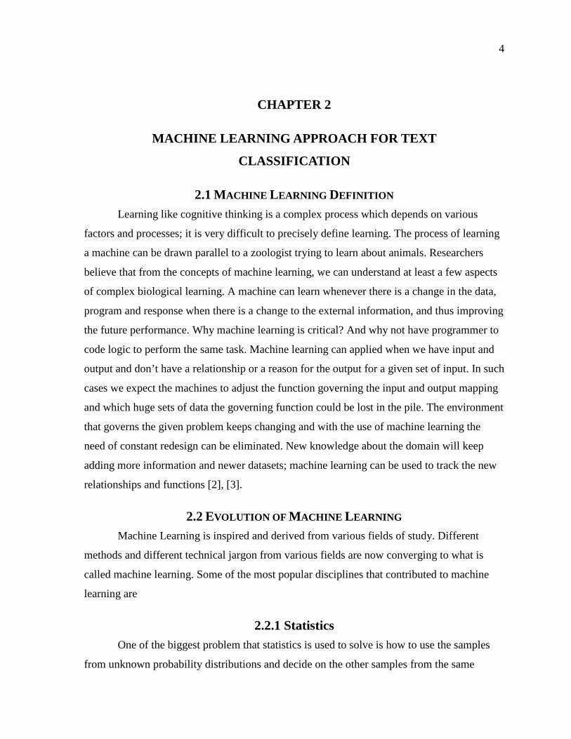
2.3 VARIETIES OF MACHINE LEARNING Machine Learning can be broadly classified into two types supervised learning and

unsupervised learning. Let us consider the some set of points in a 2-D space illustrated in

Figure 2.1. The First set of points seem to be distinguishable into 2 classes while the second

is a little difficult to classify/partition, the third seems more problematic than the first two.

This is where unsupervised algorithms come in handy, they help in finding the natural

partitions in the dataset even if the data sets seem to be complex and intermixed to the naked

eye [2].

6

Figure 2.1. Clustering algorithm.

Unsupervised learning uses procedures that attempt to find natural partitions of

patterns. There are two parts:

1. The R-partition of a set S of complex unlabeled patterns where the R itself is inferred from the patterns in the dataset. The partition of S dataset into R subsets (S1; : : : ;SR;) which are mutually exclusive is called clustering. Now we have labeled subsets from the unlabeled datasets and a suitable classifier can be developed by using the training pattern in the subsets.

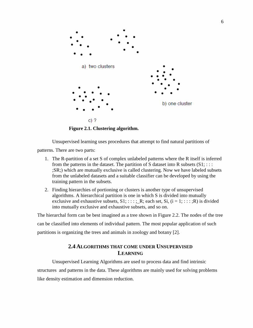
2. Finding hierarchies of portioning or clusters is another type of unsupervised algorithms. A hierarchical partition is one in which S is divided into mutually exclusive and exhaustive subsets, S1; : : : ;_R; each set, Si, (i = 1; : : : ;R) is divided into mutually exclusive and exhaustive subsets, and so on.

The hierarchal form can be best imagined as a tree shown in Figure 2.2. The nodes of the tree

can be classified into elements of individual pattern. The most popular application of such

partitions is organizing the trees and animals in zoology and botany [2].

2.4 ALGORITHMS THAT COME UNDER UNSUPERVISED LEARNING

Unsupervised Learning Algorithms are used to process data and find intrinsic

structures and patterns in the data. These algorithms are mainly used for solving problems

like density estimation and dimension reduction.

7

Figure 2.2. Hierarchical clustering.

2.4.1 Clustering The task of assigning a set/group of data sets into groups is called as cluster analysis.

Clustering is generally done in such a way that the objects in the group are similar to each

other and share common properties [2].

Clustering is a group of clusters; this group of clusters covers all objects in a dataset.

Apart from the grouping the objects in clusters, there is generally a relationship between

different clusters, like a hierarchy of clusters embedded within each other.

Hard clustering is when each object belongs to a cluster or not soft clustering (also

fuzzy clustering: each object belongs to each cluster to a certain degree, e.g. a likelihood of

belonging to the cluster).

Clustering algorithms can be categorized based on their cluster model, as listed

above. The following overview will only list the most prominent examples of clustering

algorithms, as there are probably a few dozen published clustering algorithms [2].

2.4.2 K-Means Clustering It is one of the most sought after cluster analysis derived from statistics and data

mining. This method is used to partition n objects into k clusters in which every object

8

belongs to the cluster with the nearest mean. The data space is divided into voronoi spaces

for K-means clustering.

K-means is a computationally NP problem; however there are heuristic algorithms to

converge fast to local optimum [2].

2.4.3 Hierarchical Clustering It is a method of cluster analysis where there is a hierarchy of clusters is built. There

are two types of hierarchical clustering.

2.4.3.1 AGGLOMERATIVE The “bottom up” approach is adopted in Agglomerative clustering, where each

observation is analyzed in its own cluster and later pairs of clusters are merged together to

move one hierarchy up. The time complexity of this algorithm is and thus it is difficult and

slow to work with large datasets

2.4.3.2 DIVISIVE This is a “top down” approach: all observations start in one cluster, and splits are

performed recursively as one moves down the hierarchy. In general, the merges and splits are

determined in a greedy manner. Dendogram is used to present the hierarchical clustering.

Divisive clustering with an exhaustive search is , which is even worse.

2.4.4 Blind Signal Separation The separation of set of signals from a set of mixed signals is Blind signal separation,

it is assumed that we don’t have any information about the source signals and the mixing

process. Two most popular Blind signal separations are:

1. Principal component analysis

2. Singular value decomposition

2.4.4.1 PRINCIPAL COMPONENT ANALYSIS Orthogonal transformation for the basis of principal component analysis (PCA). The

orthogonal transformation is transforms the set of observations of related values to set of

uncorrelated values/variables called principal components. The number of principal

components is always lesser than the original variables.

9

The first principal component has the highest variance which accounts for variability

in the data, the next components have the higher variance with a constraint that it is

orthogonal to preceding components. Principal components are guaranteed to be independent

only if the data set is jointly normally distributed. PCA is sensitive to the relative scaling of

the original variables. Depending on the field of application, it is also named the discrete

Karhunen-Loeve transform (KLT) [8].

2.4.4.2 SINGULAR VALUE DECOMPOSITION ANALYSIS

The singular value decomposition (SVD) is a factorization of a real or complex

matrix, with many useful applications in signal processing and statistics. Formally, the

singular value decomposition of an m×n real or complex matrix M is a factorization of the

form where U is an m×m real or complex unitary matrix, Σ is an m×n rectangular diagonal

matrix with nonnegative real numbers on the diagonal, and V* (the conjugate transpose of V)

is an n×n real or complex unitary matrix. The diagonal entries Σi,i of Σ are known as the

singular values of M. The m columns of U and the n columns of V are called the left singular

vectors and right singular vectors of M, respectively [1].

2.5 SUPERVISED LEARNING It is a machine learning technique of inferring a function from a training data. The

training data consisting of a training data set. In supervised learning set each example has an

input vector and an expected output result. An inferred function is developed by analyzing

the training data and produces an inferred function which is called a classifier. The inferred

function will predict the correct output value for any valid [2].

2.5.1 Steps to Solve Supervised Learning To solve any classification problem with Supervised Learning algorithms we should

perform the following steps:

• Training data to apply on the algorithm. Before actually implementing the algorithm we need to decide on the data that has to be used for training the algorithm. For example in text classification, it could be a word, a phrase, or two words at a time and so on.

10

• Training set gathering. The training dataset we use need to resemble the actual word data for the function to be appropriate. The training dataset should be as complete as possible.

• Input Feature. The accuracy of the function that is being developed depends on how well the input dataset is represented. The input data set is transformed into a feature vector; the features should exactly and precisely represent the input dataset. The number of features should not be too large because of the curse of dimensionality, but should contain enough information to actually predict the output.

• Determine the structure of the learned function and corresponding learning algorithm. For example, the engineer may choose to use support vector machines or Bayesians classifier.

• After completing the design, the learning algorithm is run through the training set, the supervised learning algorithm require to determine certain parameters. The parameters must be adjusted by varying the parameters.

• Evaluating the accuracy, after the algorithm is subjected to the gathered training set, the performance of the resulting function should be measured on a test set that is separate from the training set.

2.5.2 Supervised Learning Algorithms There are a wide range of algorithms available for supervised learning; each has its

pros and cons. There is nothing like an ideal supervised learning algorithm that can solve all

problems and can be applied to all datasets. Some of the most popular algorithms are as

follows.

2.5.2.1 NAÏVE BAYES It is the most popular and widely used algorithm primarily for classification

problems. The assumption that the independent variables are statistically independent is the

main idea behind this algorithm. The simplicity of this in terms of comprehension and use

made it widely popular. Naïve Bayes algorithm is ideal when the input feature vector is really

high. This simple algorithm outperforms most complex algorithms because of its simple

assumption of independent variables. A variety of methods exist for modeling the conditional

distributions of the inputs including normal, lognormal, gamma, and Poisson [9].

2.5.2.2 SUPPORT VECTOR MACHINES This method performs regression and classification by making non linear boundaries

in the given dataset. Because of complex and intermixed datasets, SVN provides great

11

flexibility in building a classifier. There are several types of support vector models including

linear, polynomial, RBF and sigmoid [10].

2.5.2.3 K-NEAREST NEIGHBORS (KNN) In contrast to the statistical methods, KNN is a memory based method and requires

not training. KNN is based on the assumption that the objects that are located close belong to

a certain category. KNN prediction is based on set of prototypes examples based on the

majority vote and average regression over a KNN prototypes [11], [12].

12

CHAPTER 3

DATA SET, APPROACH, PREPROCESSING

3.1 DATASET FOR TEXT MINING The 20 Newsgroups data set is a collection of 20,000 documents partitioned into

20 different categories. This dataset has been extremely popular for text mining and text

classification purposes. The original source of this data set is Tom Mitchell from Carnegie

Mellon University.

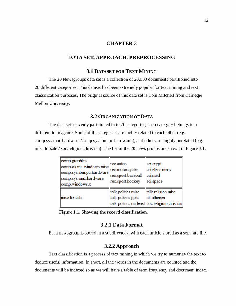
3.2 ORGANIZATION OF DATA The data set is evenly partitioned in to 20 categories, each category belongs to a

different topic/genre. Some of the categories are highly related to each other (e.g.

comp.sys.mac.hardware /comp.sys.ibm.pc.hardware ), and others are highly unrelated (e.g.

misc.forsale / soc.religion.christian). The list of the 20 news groups are shown in Figure 3.1.

Figure 1.1. Showing the record classification.

3.2.1 Data Format Each newsgroup is stored in a subdirectory, with each article stored as a separate file.

3.2.2 Approach Text classification is a process of text mining in which we try to numerize the text to

deduce useful information. In short, all the words in the documents are counted and the

documents will be indexed so as we will have a table of term frequency and document index.

13

Once we have the matrix of the term frequencies and document index, various well known

analytic algorithms can be implemented for text classification. We can use any of the

supervised and unsupervised learning methods available to draw predictive conclusions on

the test data [13].

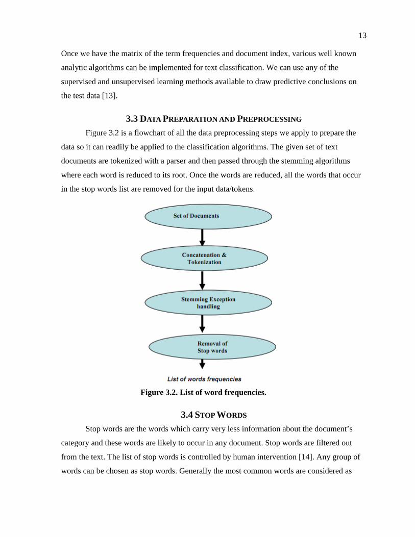
3.3 DATA PREPARATION AND PREPROCESSING Figure 3.2 is a flowchart of all the data preprocessing steps we apply to prepare the

data so it can readily be applied to the classification algorithms. The given set of text

documents are tokenized with a parser and then passed through the stemming algorithms

where each word is reduced to its root. Once the words are reduced, all the words that occur

in the stop words list are removed for the input data/tokens.

Figure 3.2. List of word frequencies.

3.4 STOP WORDS Stop words are the words which carry very less information about the document’s

category and these words are likely to occur in any document. Stop words are filtered out

from the text. The list of stop words is controlled by human intervention [14]. Any group of

words can be chosen as stop words. Generally the most common words are considered as

14

stop words, words like at, the, is, which and on etc. Source for the collection of stop words

combined with my list, my dataset of stop words comprises around 1293 which we port in a

MySQL table named stop words [15], [16], [17], [18].

3.5 STEMMER ALGORITHM Stemming is another information retrieval process for reducing the feature space of

the data set. In this process the words are reduced to their stem or root. Ideally a stemming

algorithm should reduce the words fishing, fished, fish and fisher to the root word fish. A

stemmer for English, for example, should identify the string “cats” (and possibly “catlike”,

“catty”, etc.) as based on the root “cat”, and “stemmer”, “stemming”, “stemmed” as based on

“stem”. A stemming algorithm reduces the words “fishing”, “fished”, “fish”, and “fisher” to

the root word, “fish”.

Stemming as a normalization process is used in majority of the text mining problems

for the reason that the total number of terms in the data set are reduced considerably and thus

the complexity of the data set and computational times come down. The algorithm for the

porter-stemmer is as follows. The two points to be noted about this algorithm are:

1. The suffix is being removed only to improve the IR performance and is not a linguistic exercise, as the suffix stripping cannot be controlled depending on the words and document,

2. If connections and connection are two words, they will be conflated to connection, so is the case with relate and relativity.

Stemming is done with a list of suffix and rules for each suffix, and with more

complicated rule and suffix there is equal chanced of degradation of the information

available in the dataset. For example, wander, will be conflated to wand, which is not the

stem word for wander. Therefore, with the chances of degradation being equally likely, I

have chose a simple stemmer which does not apply complex rules and suffixes [18], [19].

3.6 ALGORITHM The algorithm and the rules applied are the result of a study from the Porter-Stemmer

technical paper from Cambridge University. Any alphabet other than A, E, I, O, U and Y

preceded by a consonant is considered as constant, any thing other than consonant is

considered as vowel. Now a consonant is considered as c and a list of consonants like cccc…

15

is denoted by C and a list of vowels vvvv… id denoted as V, a word can be denoted by any

of the following four forms: CVCV ... C; CVCV ... V; VCVC ... C; or VCVC ... V.

Any word can be represented by the single form

[C]VCVC ... [V]

The square brackets are arbitrary, this may be represented as

[C](VC){m}[V]

where VC is repeated m times. The rules can be given in the form

(condition) S1 -> S2

This means if the suffix is S1 and the word satisfies the condition, the suffix is replaced by

S2. The condition part may also contain

*S - the stem ends with S (and similarly for the other letters)

*v* - the stem contains a vowel.

*d - the stem ends with a double consonant (e.g. -TT, -SS).

*o - the stem ends cvc, where the second c is not W, X or Y (e.g. -WIL, -HOP).

Only te longest matching s1 for a give word is taken if we have multiple options that

complies with S1, For example: SSES -> SS; IES -> I; SS -> SS; and S ->.

Here the conditions are all null. CARESSES maps to CARESS since SSES is the longest

match for S1. Equally CARESS maps to CARESS (S1=`SS’) and CARES to CARE

(S1=`S’). We deal with plural forms and past participles here.

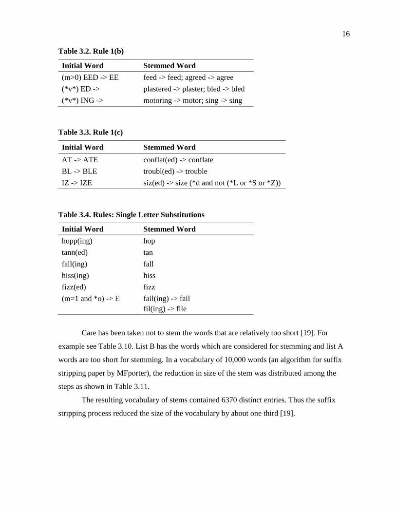
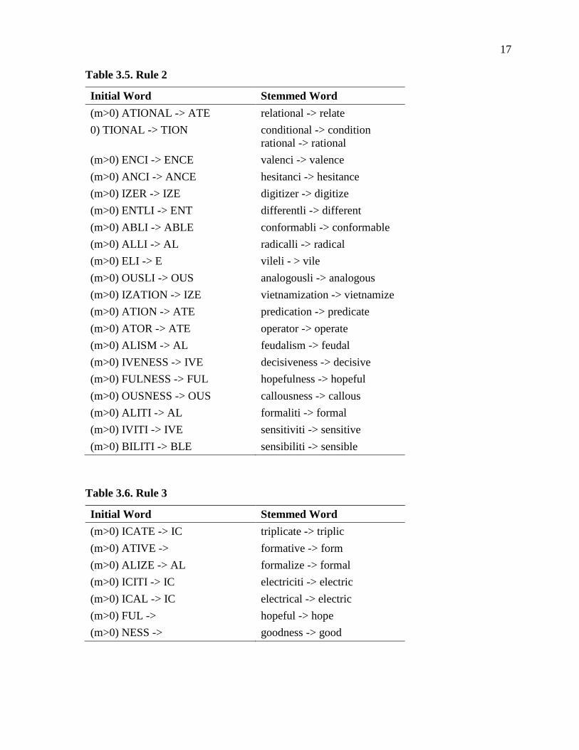
3.8 RULES Rule 1 is divided into 4 subparts as seen in Tables 3.1 to 3.4. If either of second and

third subparts of rule 1 complies, we implement the rule shown in Table 3.3. The next set of

rules for stemming is as shown in Table 3.5. Rule 3 is shown in Table 3.6. Rule 4 is shown in

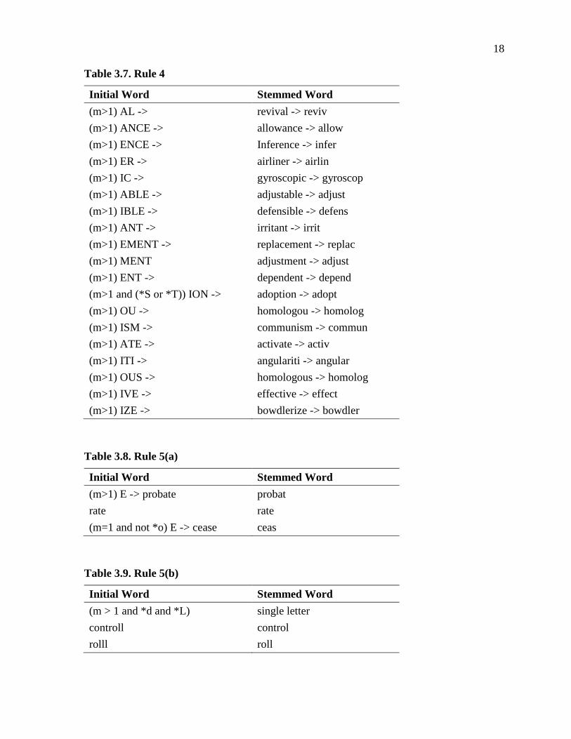
Table 3.7. Rule 5 is shown in Tables 3.8 and 3.9.

Table 3.1. Rule 1(a)

Initial Word Stemmed Word SSES -> SS caresses -> caress IES -> I ponies -> poni ; ties -> ti SS -> SS caress -> caress S -> cats -> cat

16

Table 3.2. Rule 1(b)

Initial Word Stemmed Word (m>0) EED -> EE feed -> feed; agreed -> agree (*v*) ED -> plastered -> plaster; bled -> bled (*v*) ING -> motoring -> motor; sing -> sing

Table 3.3. Rule 1(c)

Initial Word Stemmed Word AT -> ATE conflat(ed) -> conflate BL -> BLE troubl(ed) -> trouble IZ -> IZE siz(ed) -> size (*d and not (*L or *S or *Z))

Table 3.4. Rules: Single Letter Substitutions

Initial Word Stemmed Word hopp(ing) hop tann(ed) tan fall(ing) fall hiss(ing) hiss fizz(ed) fizz (m=1 and *o) -> E fail(ing) -> fail

fil(ing) -> file

Care has been taken not to stem the words that are relatively too short [19]. For

example see Table 3.10. List B has the words which are considered for stemming and list A

words are too short for stemming. In a vocabulary of 10,000 words (an algorithm for suffix

stripping paper by MFporter), the reduction in size of the stem was distributed among the

steps as shown in Table 3.11.

The resulting vocabulary of stems contained 6370 distinct entries. Thus the suffix

stripping process reduced the size of the vocabulary by about one third [19].

17

Table 3.5. Rule 2

Initial Word Stemmed Word (m>0) ATIONAL -> ATE relational -> relate 0) TIONAL -> TION conditional -> condition

rational -> rational (m>0) ENCI -> ENCE valenci -> valence (m>0) ANCI -> ANCE hesitanci -> hesitance (m>0) IZER -> IZE digitizer -> digitize (m>0) ENTLI -> ENT differentli -> different (m>0) ABLI -> ABLE conformabli -> conformable (m>0) ALLI -> AL radicalli -> radical (m>0) ELI -> E vileli - > vile (m>0) OUSLI -> OUS analogousli -> analogous (m>0) IZATION -> IZE vietnamization -> vietnamize (m>0) ATION -> ATE predication -> predicate (m>0) ATOR -> ATE operator -> operate (m>0) ALISM -> AL feudalism -> feudal (m>0) IVENESS -> IVE decisiveness -> decisive (m>0) FULNESS -> FUL hopefulness -> hopeful (m>0) OUSNESS -> OUS callousness -> callous (m>0) ALITI -> AL formaliti -> formal (m>0) IVITI -> IVE sensitiviti -> sensitive (m>0) BILITI -> BLE sensibiliti -> sensible

Table 3.6. Rule 3

Initial Word Stemmed Word (m>0) ICATE -> IC triplicate -> triplic (m>0) ATIVE -> formative -> form (m>0) ALIZE -> AL formalize -> formal (m>0) ICITI -> IC electriciti -> electric (m>0) ICAL -> IC electrical -> electric (m>0) FUL -> hopeful -> hope (m>0) NESS -> goodness -> good

18

Table 3.7. Rule 4

Initial Word Stemmed Word (m>1) AL -> revival -> reviv (m>1) ANCE -> allowance -> allow (m>1) ENCE -> Inference -> infer (m>1) ER -> airliner -> airlin (m>1) IC -> gyroscopic -> gyroscop (m>1) ABLE -> adjustable -> adjust (m>1) IBLE -> defensible -> defens (m>1) ANT -> irritant -> irrit (m>1) EMENT -> replacement -> replac (m>1) MENT adjustment -> adjust (m>1) ENT -> dependent -> depend (m>1 and (*S or *T)) ION -> adoption -> adopt (m>1) OU -> homologou -> homolog (m>1) ISM -> communism -> commun (m>1) ATE -> activate -> activ (m>1) ITI -> angulariti -> angular (m>1) OUS -> homologous -> homolog (m>1) IVE -> effective -> effect (m>1) IZE -> bowdlerize -> bowdler

Table 3.8. Rule 5(a)

Initial Word Stemmed Word (m>1) E -> probate probat rate rate (m=1 and not *o) E -> cease ceas

Table 3.9. Rule 5(b)

Initial Word Stemmed Word (m > 1 and *d and *L) single letter controll control rolll roll

19

Table 3.10. Words Ending with –ATE in Two Lists

List A List B ------ ------ RELATE DERIVATE PROBATE ACTIVATE CONFLATE DEMONSTRATE PIRATE NECESSITATE PRELATE RENOVATE

Table 3.11. Suffix Stripping of a Vocabulary of 10,000 Words

Step Number of Words Reduced 1 3597 2 766 3 327 4 2424 5 1373

Number of words not reduced 3650

3.9 WORD FREQUENCY AND VOCABULARY After the stop words processing and stemming the words, the input dataset has come

down by a considerable amount. For every document in the training data set, the word

frequencies are calculated per document. For example for the documents d1, d2 … dn we

have a vector for each document v1, v2, … vn. Each vector consists of the words in the

document and its corresponding frequency per document.

3.10 DESIGN DECISION To rule out the words that contribute too less information or the term frequencies

which skew the distribution curve, only those words are considered in the vocabulary that are

repeated more than five times in the cumulative word frequency. Finally after the

preprocessing of data and de skewing the term frequencies we end with a vocabulary of

words which are considered to build a Bayesians model for text classification [19].

20

CHAPTER 4

BAYESIAN CLASSIFIER

The Naïve Bayes classifier is the most versatile machine learning algorithm. It is

specially popular with extremely high dimensionality. Given its simplicity, it outperforms

most complex operations [11], [20], [21], [22].

Machine Learning algorithms I chose was the multinomial Naïve Bayes model, which

is a probabilistic method and is classified as supervised learning algorithm.

Mathematical foundation is the probability of a document to belong to a category c

and is computed as:

Here in the above equation, is called the probability of term , occurring in a

document c. here tk is the parameter which gives us the information of how the word tk can

be related to class c. when we have the document with tk corresponding to multiple classes,

the chose the class that evaluates to the highest priority in the above equation. Here t1, t2, t3

… tn is the vocabulary of all the training set.

At this point of time we already have the vocabulary after preprocessing the data

which is free from stop words and all the tokens are stemmed to their suffix.

The posterior probability is calculated for every category for a give document and the

category that evaluates to maximum a posterior probability ϲmap is the class that the document

is classified to

In the above equation, the conditional parameter carries weight that gives us

information and tells us if tk is big enough to consider c as its class. The prior probability

P(c), from the above equation the higher the P(c), the more are the chances for the document

21

to belong to C, a class that appears more frequently is the class that will given more weight

for a document to be classified into that class. Estimation of the parameters and .

The maximum likelihood is a probability theory which gives us the relative

frequency:

where is the number of documents in class and is the total number of documents.

We estimate the conditional probability as the relative frequency of term in

documents belonging to class :

Here is the word frequency of term t in training documents of class c that including all the

occurrences in a single document [22], [23].

To eliminate zeros we add 1 to the above equation

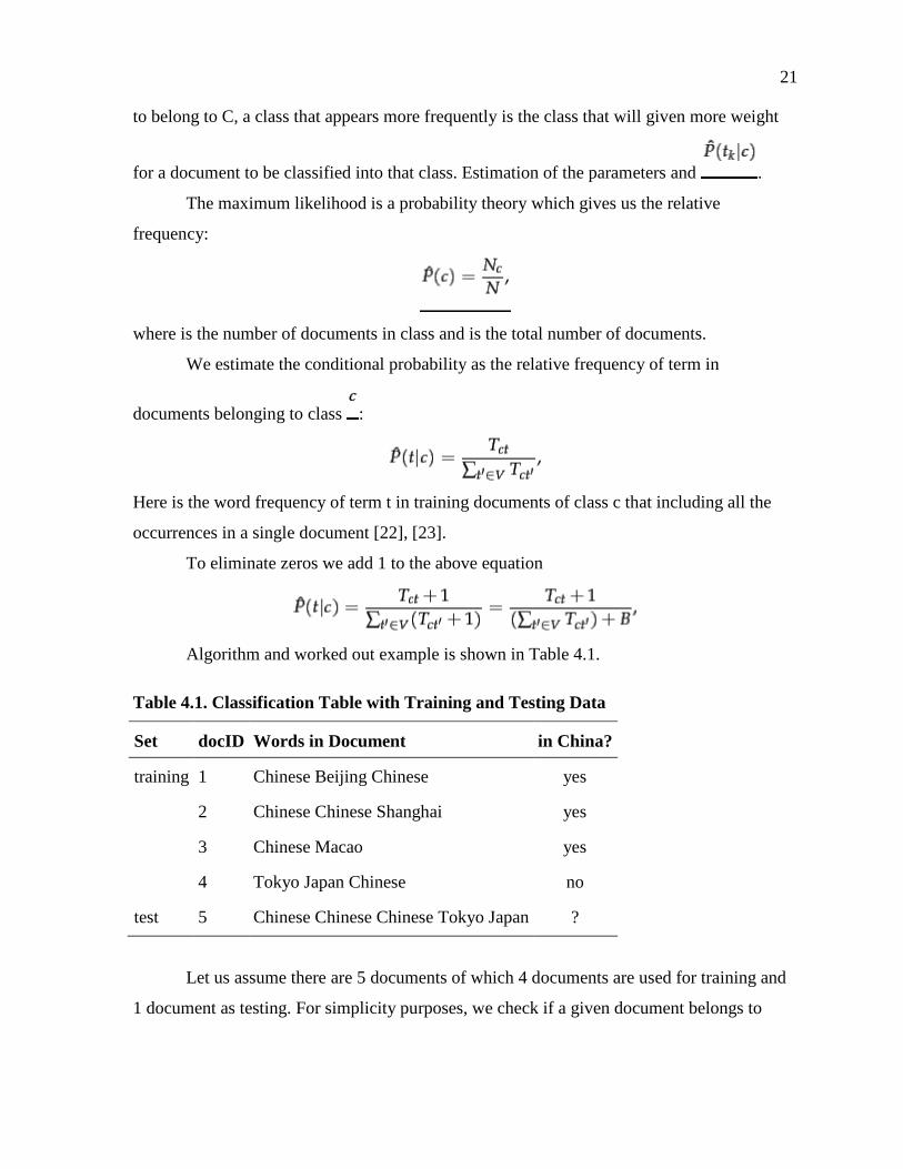
Algorithm and worked out example is shown in Table 4.1.

Table 4.1. Classification Table with Training and Testing Data

Set docID Words in Document in China?

training 1 Chinese Beijing Chinese yes

2 Chinese Chinese Shanghai yes

3 Chinese Macao yes

4 Tokyo Japan Chinese no

test 5 Chinese Chinese Chinese Tokyo Japan ?

Let us assume there are 5 documents of which 4 documents are used for training and

1 document as testing. For simplicity purposes, we check if a given document belongs to

22

class china. Document 1, 2, and 3 belong to class china, document 4 does not belong to class

china, and we need to classify the document 5. Steps are as follows:

1. Now we have the count of a token in the training set, in this example for the word Chinese the is 5.

2. We need to have the count of all the vocabulary of the whole training data set, i.e. each token is counted only once and in this example. We have Chinese, Beijing, Shanghai, Macao, Japan, Tokyo which accounts to value 6.

3. We need to have a count of all the occurrences of all the token in the training data set for a given class. For example, considering the first three documents belong to a class china we need to have the count of all the tokens including repetitions, Here in the document 1, 2 and 3 we count Chinese Beijing Chinese from document 1; Chinese Chinese Shanghai from document 2; Chinese Macao from document 3.

All the tokens from the above 3 documents sum up to 8. And the tokens from

document 4 Tokyo Japan Chinese accounts to 3. Now, for the test data, having the tokens

Chinese Chinese Chinese Tokyo Japan we need to calculate the Cmap:

and

Thus, we have the following calculations:

We then get:

4.1 PSEUDO CODE, IMPLEMENTATIONS AND INTERMEDIARY RESULTS

We build a parser to convert the text documents to vectors, the pseudo code to

convert the documents to words is presented. After the tokenizing, the stop words and

stemming algorithms are applied and the intermediary results are presented.

23

4.1.1 Parser Parsing is a process of converting text into tokens/words, the input to the parser is the

data set of 20,000 documents which are converted to tokens/words.

• Input: All the 20,000 news text documents

• Output: Words which are tokenized and processed for special symbols and removed them.

Parser and tokenizing pseudo code applied for both testing data and training data:

1. Read all the 20,000 documents as input to the parser

2. Tokenize the documents with by words

4.1.2 Pseudo Code for Parsing Here is pseudo code for building the parser:

For each document For each line each_word = each_Line.split(“ “); store in a Mysql table categoryname_vocab end end

The list of documents are converted into single words by splitting them at spaces and

new lines. The words are stored in mysql table, and after tokenizing the resultant words are

stripped off the special characters and strings with help of patterns in regular expressions.

1. Refining the words and removing the special characters and symbols which add up to the noise in the training dataset, this step is specially important as the documents are news groups picked up from the Internet, they have a lot fo special characters and meaningless information.

Regular Expression patters which are excluded from the text are:

pattern1=“,|\”||’|/|\\(|\\)|>|<|>>|\\?|\\*|\\[|\\]|\\*|_|!|#|%|\\{|\\}|`|^|:|;|=“ pattern2=“([\\w-]+(?:\\.[\\w-]+)*@(?:[\\w-]+\\.)+\\w{2,7})\\b”; pattern3=“^\\’“; pattern4=“\\’$”; pattern2=“[\\^]+”; pattern3=“\\|”; pattern4=“=“; pattern5=“\\\\”; pattern6=“\\|”; pattern7=“=“; pattern8=“!”; pattern9=“[~]+”; pattern10=“,|:|;|&|@|\\?|\\+”;.

24

2. Finally after replacing all the above pattern with empty string, split for spaces and trim the word such that there are no leading and trailing spaces.

4.2 TOKENIZATION OF TRAINING DATASET For each token generated in Step 2 check for the patterns listed above. Replace the

pattern with space. Trim each token for leading and trailing spaces. Store the refined tokens

in a new table.

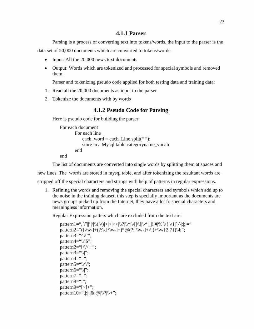
After the initial tokenization, the total number of tokens with repetitions in the

training data is stored in the table words_vocab accounting to 638021. The total number of

token in all the testing documents accounted for about 1.9 million. See Table 4.2.

Table 4.2. Database Tables with Number of Tokens

Database Tables/Category No. of Words/Features/Tokens Atheism_vocab 198002 Autos_vocab 121898 Baseball_vocab 127625 Christian_vocab 235371 Crypt_vocab 188176 Electronics_vocab 241469 Forsale_vocab 141257 Graphics_vocab 396076 Guns_vocab 394126 Hockey_vocab 304438 Ibm_pc_hardware_vocab 230626 Mac_hardware_vocab 104500 Med_vocab 165816 Motorcycles_vocab 109173 Ms_windows_vocab 132695 Politics_mideast_vocab 301993 Politics_misc_vocab 251888 Religion_misc_vocab 205956 Space_vocab 179892 Windows_x_vocab 181011

25

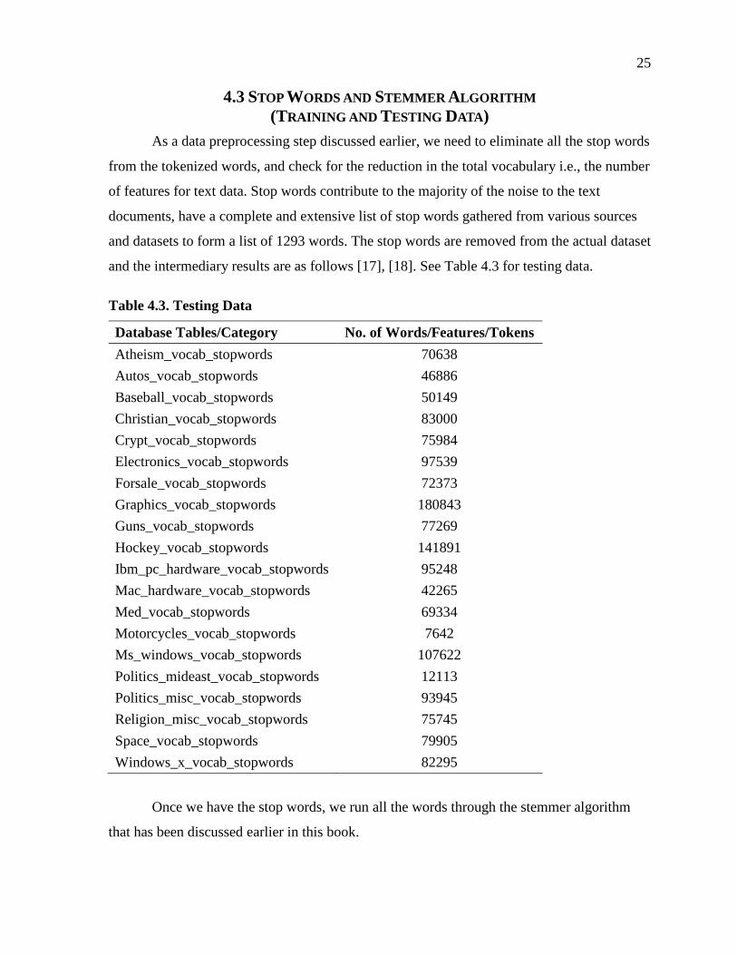
4.3 STOP WORDS AND STEMMER ALGORITHM (TRAINING AND TESTING DATA)

As a data preprocessing step discussed earlier, we need to eliminate all the stop words

from the tokenized words, and check for the reduction in the total vocabulary i.e., the number

of features for text data. Stop words contribute to the majority of the noise to the text

documents, have a complete and extensive list of stop words gathered from various sources

and datasets to form a list of 1293 words. The stop words are removed from the actual dataset

and the intermediary results are as follows [17], [18]. See Table 4.3 for testing data.

Table 4.3. Testing Data

Database Tables/Category No. of Words/Features/Tokens Atheism_vocab_stopwords 70638 Autos_vocab_stopwords 46886 Baseball_vocab_stopwords 50149 Christian_vocab_stopwords 83000 Crypt_vocab_stopwords 75984 Electronics_vocab_stopwords 97539 Forsale_vocab_stopwords 72373 Graphics_vocab_stopwords 180843 Guns_vocab_stopwords 77269 Hockey_vocab_stopwords 141891 Ibm_pc_hardware_vocab_stopwords 95248 Mac_hardware_vocab_stopwords 42265 Med_vocab_stopwords 69334 Motorcycles_vocab_stopwords 7642 Ms_windows_vocab_stopwords 107622 Politics_mideast_vocab_stopwords 12113 Politics_misc_vocab_stopwords 93945 Religion_misc_vocab_stopwords 75745 Space_vocab_stopwords 79905 Windows_x_vocab_stopwords 82295

Once we have the stop words, we run all the words through the stemmer algorithm

that has been discussed earlier in this book.

26

Calculating the actual vocabulary (Training Data) is as follows. The total number of

tokens in the training data is stored in the table words_vocab accounting to 221389. Now

from all the documents, we need to get the count of the unique words in the database this

accounts to the actual vocabulary and also considered as the features space in Machine

learning Jargon. So as it is really important to keep the feature space as low as possible which

will retain the maximum information about the class, we have to make certain assumption

about it.

All the unique words from the tables discussed previously are stored in the Database

table words_freq. Select count(*) from words_vocab gives 221389, which is still high and it

contributes to a computational over head. However, only those words which have appeared

more than 5 times are considered for the vocabulary and is the actual feature space for this

specific dataset. All the words that have appeared more than 5 times are recorded in the

database words_freq5. Select count(*) from words_freq5 gives 55809, which I feel is

computationally acceptable compared to 221389. Now the actual vocabulary /Feature space

is calculated by Select distinct(word) from word_freq5, which gives us a result of 18958.

This set of words in the words_freq5 is used to calculate the apriori probability.

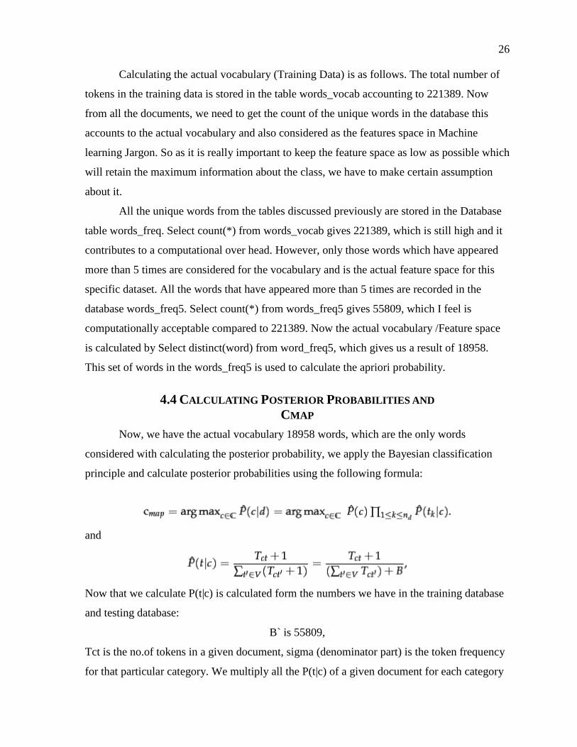
4.4 CALCULATING POSTERIOR PROBABILITIES AND CMAP

Now, we have the actual vocabulary 18958 words, which are the only words

considered with calculating the posterior probability, we apply the Bayesian classification

principle and calculate posterior probabilities using the following formula:

and

Now that we calculate P(t|c) is calculated form the numbers we have in the training database

and testing database:

B` is 55809,

Tct is the no.of tokens in a given document, sigma (denominator part) is the token frequency

for that particular category. We multiply all the P(t|c) of a given document for each category

27

and classify the document to that category which gives us the highest cmap. Here is the result

of all the documents and categories that have been classified appropriately and the

documents that have been misclassified.

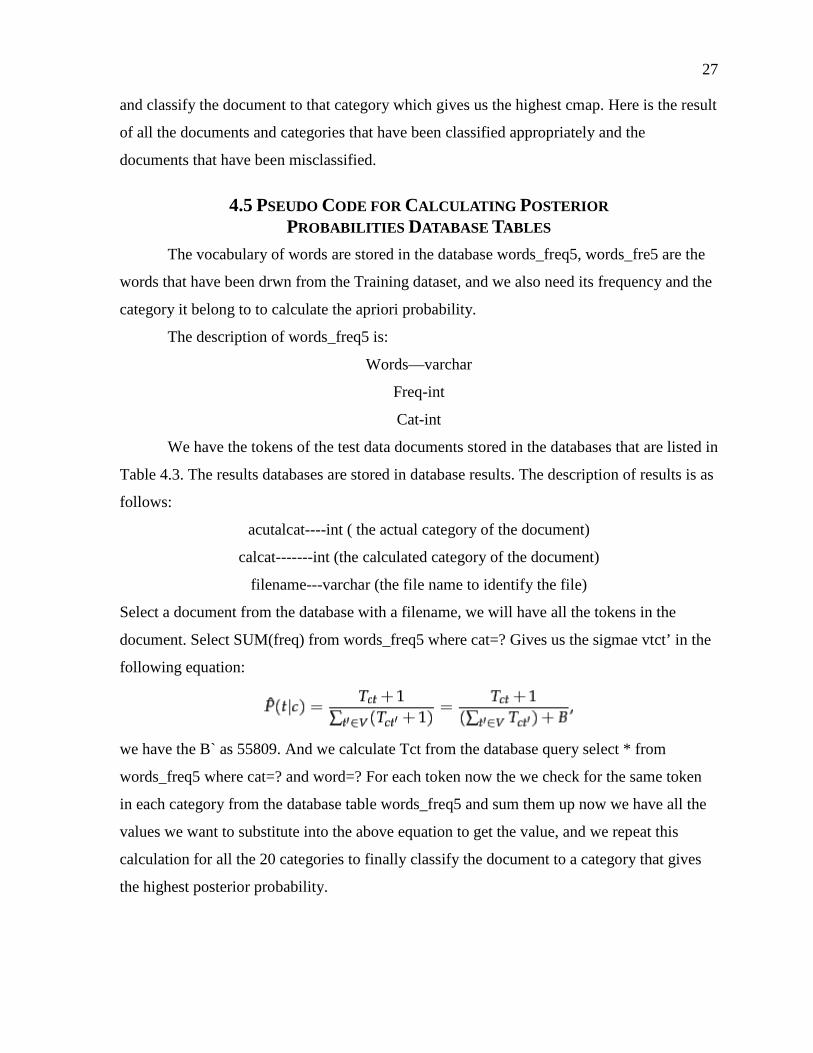
4.5 PSEUDO CODE FOR CALCULATING POSTERIOR PROBABILITIES DATABASE TABLES

The vocabulary of words are stored in the database words_freq5, words_fre5 are the

words that have been drwn from the Training dataset, and we also need its frequency and the

category it belong to to calculate the apriori probability.

The description of words_freq5 is:

Words—varchar

Freq-int

Cat-int

We have the tokens of the test data documents stored in the databases that are listed in

Table 4.3. The results databases are stored in database results. The description of results is as

follows:

acutalcat----int ( the actual category of the document)

calcat-------int (the calculated category of the document)

filename---varchar (the file name to identify the file)

Select a document from the database with a filename, we will have all the tokens in the

document. Select SUM(freq) from words_freq5 where cat=? Gives us the sigmae vtct’ in the

following equation:

we have the B` as 55809. And we calculate Tct from the database query select * from

words_freq5 where cat=? and word=? For each token now the we check for the same token

in each category from the database table words_freq5 and sum them up now we have all the

values we want to substitute into the above equation to get the value, and we repeat this

calculation for all the 20 categories to finally classify the document to a category that gives

the highest posterior probability.

28

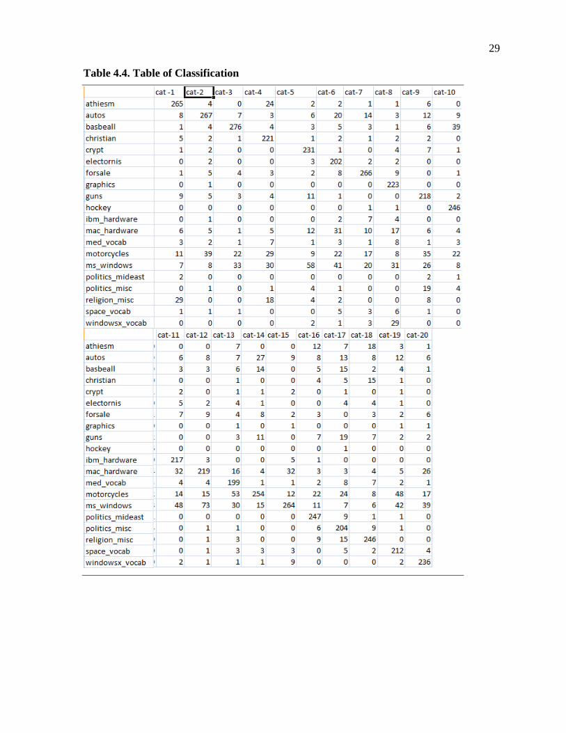
4.6 RESULTS AND GRAPH Figure 4.1 summarizes the accuracy plot classification of various categories based on

the data set I have considered. The plot in Figure 4.1 suggests that documents that belong to

the category of atheism, baseball and windows texts are classified with a better efficiency as

their data sets are better trained. The accuracy of documents is also a function of the

correlation between the various categories that are to be classified. As we can observe that in

the case of some categories the texts have been grouped in different categories owing to

similarities in their feature space. It is expected that if the trained data set is modified there

can be an increased efficiency with classification. It can be observed from Table 4.4 of

calculations that documents that contain similar feature sets tend to be misclassified which

accounts for the drop in efficiency to 75%.

Figure 4.1. Accuracy plot of classification.

We can infer that the Bayesian Classifier is robust against real data noise, it assumes

that the feature space attributes are independent and performed reasonable well in classifying

the text even when the attribute dependencies are strong. The Bayesian Classifier has a clear

edge over other complex algorithms when we have smaller training data and for text

classification with a smaller training dataset the learning speed can be really healthy.

Acc

ura

cy o

f cla

ssif

icat

opn

(%

)

Category

Accuracy plot of classification

29

Table 4.4. Table of Classification

30

CHAPTER 5

CONCLUSION

The task of assigning a document to a predefined category is Text Classification. If

we have n documents d1, d2, d3 … dn to be categorized into m categories c1, c2 … cm,

where D={d1,dn} and C={c1,cm} there will be a variable X indicating a decision that di

belongs to cj and a variable value Y indicating a decision that di does not belong to cj.

In Chapter 2, we discussed about the various Machine learning algorithms and

techniques available to solve a wide variety of real world classification problem. We learnt

that a Machine learning algorithm has been derived from various backgrounds like statistics,

neural networks, and probability theory. We also discussed about supervised and

unsupervised algorithms, 90% of all machine learning algorithms are either classified under

supervised or unsupervised algorithms.

In Chapter 3, we talked about the dataset used for applying the machine learning

algorithm, the dataset is the yahoo 20,000 news group, we talked about the data

preprocessing algorithms, the stop-word elimination algorithm and stemmer algorithm which

are widely used in Natural Language processing.

In Chapter 4, we discussed about the Bayesian Algorithm, which the most popular

algorithm in the Machine learning field, this chapter also has the pseudo codes for the

stemmer, stop words and Bayesian algorithm implementation and the intermediary results,

which helps us understand the importance of each of these algorithms.

31

CHAPTER 6

FUTURE WORK

Now that we have successfully classified the documents with a reasonable accuracy,

there is still scope for better efficiencies. The efficiency can certainly be improved by

providing a dataset that covers the feature space required to classify the documents.

We know that the apriori probability is the most important factor to calculate the

posterior probability, It is assumed that the apriori probability is constant throughout the

classification process. However we can implement an adaptive apriori probability, where

after successfully classifying the test document, this document will contribute to the apriori

probability and likelihood rations, this gives us a great learning algorithm if the training

dataset available is very limited and later on the testing document outnumbers the training

dataset.

Apart from the Adaptive Bayesian probability, there are algorithms that can be used

for data preprocessing and classification algorithms.

A few data preprocessing techniques available for natural language processing are:

1. Chi Square feature extraction

2. Principal components analysis

3. Kernel PCA

4. Latent semantic analysis

There are as well a lot of classification algorithms apart from Bayesians:

1. Neural networks

2. Kernel Estimators

3. Nearest Neighbor Algorithm

4. Learning Automata.

It will be interesting to see how each of the classification performs with each of the

data preprocessing techniques.

Implementation feasibility includes document classification. Document classification

is a computation intensive process, and it take high speed machines to solve real word

32

problems in realistic time lines. I see Hadoop, map-reduce architecture as a solution to

implement the data preprocessing algorithms and classification algorithms, it is the most

economical and a practical approach to deal with huge data sets and millions of

computations.

33

BIBLIOGRAPHY

[1] Paul Bennett. 20-760: Web-Based Information Architectures July 23, 2002. http://users.softlab.ntua.gr, accessed Feb. 2012.

[2] Nils J. Nilsson. Introduction to Machine Learning, Robotics Laboratory, Department of Computer Science, 2005. http://robotics.stanford.edu/~nilsson/MLBOOK.pdf, accessed Feb. 2012.

[3] StatSoft. Naive Bayes Classifier: Technical Notes, n.d. http://www.statsoft.com/textbook/naive-bayes-classifier/#Technical Notes, accessed Nov. 2011.

[4] John G. Bollinger and Neil A. Duffie. Computer Control of Machines and Processes. Addison-Wesley, Reading, MA, 1988.

[5] A. L. Samuel. Some studies in machine learning using the game of checkers. IBM J. Res. & Devel., 3:210-229, 1959.

[6] J. G. Carbonell and T. M. Mitchell. Machine Learning: An Artificial Intelligence Approach. Morgan Kaufmann, San Mateo, CA, 1986.

[7] J. R. Quinlan. Learning logical definitions from relations. Machine Learning, 5:266, 1990.

[8] Christopher D. Manning, Prabhakar Raghavan and Hinrich Schütze. Introduction to Information Retrieval. Cambridge University Press, Cambridge, MA, 2008.

[9] M. Ikonomakis, S. Kotsiantis, and V. Tampakas. Text classification using machine learning techniques. WSEAS Trans. Comp., 4(8):966-974, 2005.

[10] Paul N. Bennett. Text Categorization through Probabilistic Learning: Applications to Recommender Systems, n.d. http://www.cs.utexas.edu/~ml/papers/pbennett-ugthesis.pdf, accessed Oct. 2011.

[11] S. B. Kim, H. C. Rim, D. S. Yook, and H. S. Lim. Effective methods for improving Naive Bayes text classifiers. LNAI 2417, 414-423, 2002.

[12] Y. Bao and N. Ishii. Combining multiple kNN classifiers for text categorization by reducts. LNCS 2534:340-347, 2002.

[13] J. Rennie. 20 Newsgroups, 2008. http://people.csail.mit.edu/jrennie/20Newsgroups/, accessed June 2011.

[14] A. Vinciarelli. Noisy text categorization, pattern recognition. Proceedings from the 17th International Conference on Pattern Recognition (ICPR’04), 4:554-557, 2004.

[15] Mohammed Abdul and Wajeed T. Adilakshmi. Text classification using machine learning. Int. J. Fuzzy Logic Sys., 2:41-51, 2012.

[16] Toman Michal, Tesar Roman and Jezek Karel. Influence of word normalization on text classification. Proceedings from the 1st International Conference on

34

Multidisciplinary Information Sciences & Technologies, Merida, Spain, 2006. InSciT2006.

[17] Webconfs. Stop Words, 2006. http://www.webconfs.com/stop-words.php, accessed Aug. 2011.

[18] J. Ignacio Serrano, M. Dolores del Castillo, Jesus Oliva, and Angel Iglesias. The influence of stop-words and stemming on human text base comprehension. Proceedings of the European Perspectives on Cognitive Science, NBU Press, Sofia, Bulgaria, 2011.

[19] M. F. Porter. An algorithm for suffix stripping. Program 14(3):130-137, 1980.

[20] M. Klopotek and M. Woch. Very large Bayesian networks in text classification. LNCS 2657:397-406, 2003.

[21] Kamal Nigam, Andrew Kachites Mccallum, Sebastian Thrun, and Tom Mitchell. Text Classification from Labeled and Unlabeled Documents Using EM, 1999. http://www.kamalnigam.com/papers/emcat-mlj99.pdf, accessed on November 2011.

[22] Christopher D. Manning, Prabhakar Raghavan and Hinrich Schütze. Introduction to Information Retrieval. Cambridge University Press, London, UK, 2008.

[23] Peter Cheeseman and John Stutz. Bayesian classification (AutoClass): Theory and results. In U. Fayyad, G. Piatetsky-Shapiro, P. Smyth, and R. Uthurusamy, editors, Advances in Knowledge Discovery and Data Mining, Cambridge, MA, 1996. MIT Press.