Tetrahedron Diagram and Perturbative Calculation in...

Adv. Studies Theor. Phys., Vol. 2, 2008, no. 18, 871 - 901

Tetrahedron Diagram and Perturbative Calculation

in Chern-Simons-Witten Theory

Freddy P Zena,b,1, Jusak S Kosasiha,b,2, Asep Y Wardayaa,c,3, Triyantaa,b,4

aTheoretical Physics Laboratory, THEPI Divisionand

bINDONESIA Center for Theoretical and Mathematical Physics (ICTMP)Faculty of Mathematics and Natural Sciences, Institut Teknologi Bandung

Jl. Ganesha 10 Bandung 40132, Indonesia

cDiponegoro University,Jl. Prof. H. Soedarto, SH. Tembalang Semarang 50275, Indonesia

Abstract

We investigate extended Wilson loop operators, in particular tetra-hedron operator in (2 + 1)-dimensional Chern-Simons-Witten theory.This operator emerges naturally from the contribution terms in two-particle scattering amplitude. We evaluate this diagram non-perturbativelyin terms of vacuum expectation values of Wilson loop operators, espe-cially for gauge group SU(N) with specific choices of representations.On the other hand, we also discuss the perturbative calculation of vac-uum expectation value in this theory. We show that, up to the thirdorder, this values of unknotted Wilson loop operators are identical tothe non-perturbative result.

Keywords: Chern-Simons theory

1 Introduction

The Chern-Simons-Witten (CSW) theory has been providing many interestingtopics for both mathematics and physics. Different aspects of the theory havebeen explored, e.g. abelian and non-abelian theory with the Chern-Simonsterm, supersymmetric extension, and pure theory. Specifically, after it was

[email protected]@[email protected]@fi.itb.ac.id

872 F. P. Zen, J. S. Kosasih, A. Y Wardaya and Triyanta

pointed out that the pure theory could be relevant for knot theory [1, 2], manyresearchers have contributed to clarify the relation of CSW theory to two-dimensional, conformal field theories and to knot theory. Witten describedthe exact solution to this theory in non-perturbative case. He and othersalso showed that there is relation between this theory and the polynomialor quantum group invariants of knot in three dimensions, in particular theJones polynomial and its generalizations like the HOMFLY and the Kauffmanpolynomial invariants [3, 4, 5]. These knot polynomials can be regarded asvacuum expectation values (VEV) of Wilson loop operators in this theory.

The CSW theory also has interesting features from the perturbative pointof view and lead to Goussarov-Vassiliev or finite type invariants. Moreover,Witten’s idea was based on the validity of the path integral formulation ofthe quantized theory. By examining the existence of a quantum field theorydescription of the link invariants in perturbative framework, it turned out thatthe coefficients of the perturbative series correspond to these invariants. Theperturbative expansion of the path integral of the theory has been consideredfor flat R3 [6] and for general three-manifolds [7]. Subsequently, there wasmuch attention given to understanding the perturbative series for knots andlinks in R3 [8].

The perturbative series expansion has been studied for different gauge-fixings which lead to different representations for Vassiliev invariants. Thecovariant Landau gauge corresponds to the configuration space integrals andthe non-covariant light-cone gauge to the Kontsevich integrals. Another studiesof the perturbative series expansion in the non-covariant temporal gauge hasthe important feature that the integrals which are present in the expressionsfor the coefficients of the perturbative series expansion can be carried out. Inthis case one obtains combinatorial expressions, instead of integral ones, forVassiliev invariants and this has been shown to be the case up to order four[9]. Perturbative expansion in other gauges might also highlight other aspectsof the theory, for example in axial gauge [10] and in light-cone gauge [11]. Theinvariants obtained in the perturbative framework with different gauge-fixingare the same since the theory is gauge invariant and Wilson loops are gaugeinvariant operators.

One main issue in perturbative CSW theory is the calculability of the vac-uum expectation value of Wilson loop operator 〈W (C)〉 in the three-dimensionalfield theory framework. It turned out that 〈W (C)〉 has a meaningful pertur-bative expansion in powers of the coupling constant k−1. Although by powercounting the theory appears renormalizable, it is in fact UV finite, which meansthe β function and the anomalous dimensions of the fields vanish to all orders[12, 13]. Even, more interestingly, there is no divergences in the computationof 〈W (C)〉 in this theory. One loop renormalization constant of the theory hasbeen calculated and the result showed the existence of the famous k shift [14].

Tetrahedron diagram and perturbative calculation in CSW theory 873

Therefore, the framing has nothing to do with divergences of 〈W (C)〉, but isrelated to the self-linking problem which is topological in origin.

The mathematical establishment of relations between CSW gauge theory,topological theories in 3 manifold and knot theory is still making progress.Some recent studies include the application of Maldacena’s conjecture [15],the use of methods of stochastic analysis [16] and its connection to the Pennermodels [17].

In this paper we will evaluate the non-perturbative as well as the pertur-bative aspects of CSW theory. In non-perturbative aspect, it is shown thatthe VEV of Wilson loop operators are evaluated by using braiding formula [18]which is useful to construct algebraic relations between unknotted Wilson loopoperators. It also discussed the emergence of the extended Wilson loop oper-ators, namely baryon type [19] and tetrahedron operators [20]. Especially, wewill evaluate the tetrahedron type operator. This diagram emerges by refiningthe calculation of the gravitational scattering amplitude in previous work [21].It is important, therefore, to make it clear what contributions will be suppliedfrom these terms.

On the other hand, parallel to the non-perturbative approach, the explicitperturbative calculation of the unknotted Wilson loop operator is presentedup to the third order. The coefficients of these expansion is shown to be thesame as the non-perturbative results. After that, we also investigate the ghostand auxiliary fields contributions to the Wilson loop operator. A detailedperturbative calculation of the ghost contribution up to the second order isgiven in the Appendix A and other important integral formulas related to theframing procedure are given in Appendix B.

2 Chern-Simons Theory and Extended Wilson

Loop Operators

In this section we will present the rudimentary facts about CSW theory andto discuss the emergence of extended Wilson loop operators5. The action forthis theory in (2 + 1)-dimension is the Chern-Simons secondary characteristicclass defined by

S =k

4π

∫M

Tr(A ∧ dA+2

3A ∧A ∧ A). (1)

Here k−1 plays the role of coupling constant whereas A is a connection ona G-bundle E over a space-time three manifold M . Trace is taken over the

5One of us (FPZ) would like to thank M. Hayashi for collaboration in this part, see ref.[20]


representation of gauge group G. The partition function Z(M, k) takes theform

Z(M, k) =

∫M

[DA] eiS. (2)

Under the gauge transformation, the action will transform as

S −→ S + 2πk SWZ , (3)

where SWZ ∈ Z is the winding number of the gauge transformation.The Wilson loop operators Wρ(C), which are the basic observables of the

theory, are the most important gauge invariant operators in this theory. Theseoperators are related to the link invariants of knot theory and defined by thetrace of path-ordered exponential of the connection A along a closed loop Cwhich is embedded in M ,

Wρ(C) = Trρ

(P exp

∮C

A

), (4)

where ρ is a representation of the gauge group G (ρ is its conjugate represen-tation). Note that a closed loop C can be knotted in the three manifold.

A normalized VEV of an operator O(A) is defined as

〈O(A)〉 =Z(M, k,O)

Z(M, k, 1), Z(M, k,O) =

∫[DA] O(A)eiS. (5)

In the following we use notation for the normalized VEV of unknotted Wilsonloop operator

E0(ρ) = 〈Wρ(�)〉, (6)

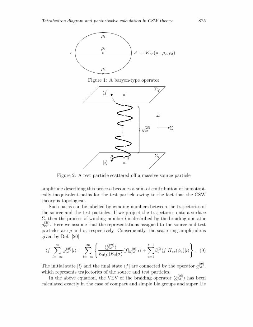
such that the VEV of the baryon-type operator (Figure 1) is denoted as

〈Kεε′(ρ1, ρ2, ρ3)〉 = δεε′√E0(ρ1)E0(ρ2)E0(ρ3), (7)

and if, for example ρ1 = id (identity representation), then from consistencycondition [19]

〈Kεε′(id, ρ3, ρ3)〉 = δεε′E0(ρ3). (8)

Now, let us imagine the following situation (see Figure 2). A test parti-cle scattered off a massive source particle situated at the spatial origin of thespace-time manifold M . Upon quantization of the test particle, the scattering


ε ε′ ≡ Kεε′(ρ1, ρ2, ρ3)

ρ1

ρ2

ρ3

Figure 1: A baryon-type operator

Σ

t

×

×|i〉

〈f | Σf

Σiσρ

⎫⎪⎪⎪⎪⎪⎪⎪⎪⎪⎪⎬⎪⎪⎪⎪⎪⎪⎪⎪⎪⎪⎭g

(2l)ρσ

•

•

Figure 2: A test particle scattered off a massive source particle

amplitude describing this process becomes a sum of contribution of homotopi-cally inequivalent paths for the test particle owing to the fact that the CSWtheory is topological.

Such paths can be labelled by winding numbers between the trajectories ofthe source and the test particles. If we project the trajectories onto a surfaceΣ, then the process of winding number l is described by the braiding operatorg

(2l)ρσ . Here we assume that the representations assigned to the source and test

particles are ρ and σ, respectively. Consequently, the scattering amplitude isgiven by Ref. [20]

〈f |∞∑

l=−∞g(2l)

ρσ |i〉 =∞∑

l=−∞

{〈g(2l)

ρσ 〉E0(ρ)E0(σ)

〈f |g(0)ρσ |i〉 +

r−1∑u=1

b(l)u 〈f |Hρσ(φu)|i〉}. (9)

The initial state |i〉 and the final state 〈f | are connected by the operator g(2l)ρσ ,

which represents trajectories of the source and test particles.In the above equation, the VEV of the braiding operator 〈g(2l)

ρσ 〉 has beencalculated exactly in the case of compact and simple Lie groups and super Lie


φu

σ σ

ρ

≡ T (φu, σ, σ|λs, ρ, ρ)

ρ

λs

Figure 3: A tetrahedron operator which contribute to scattering amplitude ofa test particle and a source particle

group, whereas b(l)u is given by

b(l)u =

r−1∑s=1

(q−Q(ρ)−Q(σ)+Q(λs))l

√E0(λs)

(E0(ρ)E0(σ))3〈T (φu, σ, σ|λs, ρ, ρ)〉, (10)

where

q = exp

(2πi

k +Q(Adj)

). (11)

Q(ρ) is the quadratic Casimir invariant of the ρ representation. T (φn, σ, σ|λρ, ρ, ρ)is a tetrahedron operator (Figure 3).

Now, we will discussed the detail calculation of the VEV of tetrahedronoperator for simple Lie group

Starting from u channel basis Hu, we can construct the following expansionof s channel Is

�s1

3

2

4

=∑u′Lsu′�u′

1

3

2

4

. (12)

If we attach the Wilson line�4 2u to the top side of both Hu and Is we will

arrive at the following relation6

6Here, we also use the following notation i ≡ ρi and i ≡ ρi(i = 1, 2, 3, 4) as representationsand its conjugate of the gauge group G attach to the Wilson lines.


�3

s

4

2

u

1

=∑u′Lsu′ �

3

u′

4

1

2u

. (13)

The loop in the Wilson line can be expressed as a single Wilson line accordingto the following identity

�4 2

u′

u

= δuu′(Uu′42)

−1�u′ (14)

then, it can be shown easily that a tetrahedron diagram can be constructedfrom baryon type diagrams as given in the following relation

�1

3

su

2

4 =∑u′Lsu′δuu′(Uu′

42)−1

3

1

u′, (15)

= Lsu(Uu42)

−1 3 u′ 1 .

Note that Usij is determined by connecting both endpoints in Eq. (14), and

therefore can be written as

Usij =

√E0(ρs)

E0(ρi)E0(ρj). (16)

Substituting this into the above tetrahedron-baryon relation, we get


⟨

�3

s

14

u

2

⟩= Lsu

(E0(4)E0(2)

E0(u)

)1/2⟨

�3

1

u

⟩(17)

which, by substituting the definition in equation (7), we finally get the VEVof tetrahedron diagram

⟨

�1

3

su

2

4

⟩= Lsu

(E0(4)E0(2)

E0(u)

)1/2

(E0(3)E0(u)E0(1))1/2, (18)

= Lsu(E0(4)E0(3)E0(2)E0(1))1/2, (19)

or

Lsu = (E0(4)E0(3)E0(1)E0(2))−1/2

⟨

�1

3

su

2

4

⟩. (20)

One can also easily see the cyclic symmetry modulo 4 of the tetrahedrondiagram as follows

�3

2

1a b

c

−→ �b

c

3 1 a

2

−→ �a

2

b 3 1

c

−→ �1

c

a b3

2

−→ �3

2

1a b

c

.

We can also define similar matrices that relates different channels

Jt =∑

u

φtMtuφ−1u HuHu =

∑t

φ−1t MtuφuJt (21)


and

Jt =∑

s

NtsφsIsIs =∑

t

Ntsφ−1s Jt, (22)

where the φ factors are defined as

φs = βsq12(Q(3)+Q(4)−Q(s), (23)

φt = βtq12(Q(t)+Q(4)−Q(1), (24)

φu = βuq12(Q(2)+Q(4)−Q(u), (25)

with symmetry factors

βa =

{+1 a is symmetric combination of two representations−1 a is antisymmetric combination of two representations.

(26)

These M and N matrices can be found by the same manner as the previousderivation of the L matrix. In summary, the matrices L,M , and N are givenby

Lsu = (E0(1)E0(2)E0(3)E0(4))−12 〈T (4, s, 2|1, u, 3)〉, (27)

Mtu = (E0(1)E0(2)E0(3)E0(4))−12 〈T (4, u, 2|3, t, 1)〉, (28)

Nts = (E0(1)E0(2)E0(3)E0(4))−12 〈T (1, t, 4|3, s, 2)〉. (29)

From the orthonormality condition of the bases, these matrices will satisfy thefollowing unitary contraints

LL† = 1,MM † = 1, NN † = 1, (30)

as well as the following orthogonality conditions, obtained from previous rela-tions

LLT = 1,MMT = 1, NNT = 1. (31)

Also, from the consistency condition, one can easily derive the following rela-tion among these matrices

NφsL = φtMφ−1u . (32)

These constraints and conditions will fix the components of these L,M , andN matrices.

Now, for example, if we choose ρ = σ = N and σ = ρ = N , where Nand N are the fundamental representation of SU(N), the VEV of tetrahedron


operator gives

Lid,S =1

E20(N)

〈T (S,N,N |id, N,N)〉 =

√E0(S)

E0(N), (33)

Lid,A =1

E20(N)

〈T (A,N,N |id, N,N)〉 =

√E0(A)

E0(N), (34)

NAdj,id =1

E20(N)

〈T (id, N,N |Adj, N,N)〉 =

√E0(Adj)

E0(N), (35)

Nid,id =1

E20(N)

〈T (id, N,N |id, N,N)〉 =1

E0(N). (36)

The above relation are consistent with the VEV of baryon type operator inequation (7)

3 Perturbative Case

In the previous chapter, we discussed the calculation of vacuum expectationvalue of extended Wilson loop operators by using unperturbative method. Thisconcept has been used for many applications in various physical conditions [10,22]. Now, we will calculate the vacuum expectation value of unknotted Wilsonloop operator 〈Wρ(�)〉 within the framework of perturbation theory. Theperturbative problem has been discussed in many papers for many differentsettings [7, 8, 12, 17, 23, 24, 25]. In this section, we use arbitrary gaugegroup and restrict the order of the calculation of 〈Wρ(�)〉 up to order (2π

k)3.

Particularly, we compare the result with the nonperturbative one for SU(N)and E6 gauge groups.

In the perturbative case, the classical CSW action (1) must undergo amodification in order to perform the quantization. We will adopt the standardFaddeev-Popov procedure, and the total action becomes [6]

Stot = SCS + Sgauge−fixing + Sghost

=k

4π

∫M3

d3x εμνρ Tr

(Aμ∂νAρ + i

2

3AμAνAρ

)

+k

4π

∫M3

d3x√g gμν Aa

μ∂νφa −

∫M3

d3x√g gμν ∂ν c

a(Dνc)a, (37)

where c and ca are Faddeev-Popov ghosts, φa is the Lagrange multiplier (aux-iliary field) and

(Dμc)a = ∂μc

a − fabcAbμc

c. (38)


Here, fabc is the structure constant of the group G and gμν is some metric onM3. The resulting propagators from eq. (37) are

⟨Aa

μ(x)Abν(y)

⟩=i

kδabεμνσ

(x− y)σ

|x− y|3 , (39)

⟨Aa

μ(x)φb(y)

⟩= − i

kδab (x− y)μ

|x− y|3 , (40)

⟨φa(x)φb(y)

⟩= 0, (41)

⟨ca(x)cb(y)

⟩= − i

4πδab 1

|x− y| . (42)

The Wilson loop operator in a representation ρ of G [5, 6] is defined as

Wρ(C) = Trρ(P exp

∮C

A)

= Trρ

[1 + i

∮C

dxμAμ(x) −∮

C

dxμ

∫ x

dyνAν(y)Aμ(x)

− i

∮C

dxμ

∫ x

dyν

∫ y

dzρAρ(z)Aν(y)Aμ(x)

+

∮C

dxμ

∫ x

dyν

∫ y

dzρ

∫ z

dwσAσ(w)Aρ(z)Aν(y)Aμ(x)

+ i

∮C

dxμ

∫ x

dyν

∫ y

dzρ

∫ z

dwσ

∫ w

dvλAλ(w)Aσ(w)Aρ(z)Aν(y)Aμ(x)

−∮

C

dxμ

∫ x

dyν

∫ y

dzρ

∫ z

dwσ

∫ w

dvλ

∫ v

duτ

× Aτ (u)Aλ(w)Aσ(w)Aρ(z)Aν(y)Aμ(x) + ...

]. (43)

All line integrals are performed on the same contour C. If an explicit param-eterizations {xμ(t) : 0 ≤ t ≤ 1} of C is used, then we will get

∮C

dxμ

∫ x

dyν =

∫ 1

0

ds

∫ s

0

dt xμ(s)xν(t), (44)

and so on.


3.1 The Ghost Fields Contribution

From eq. (37), the total quantized action contains contributions from gauge,ghost and auxiliary fields. This can be rewritten again as

Stot =

∫d3x

(k

4πc2(ρ) ε

μνρ Aaμ∂νA

aρ +

k

4πAa

μ∂μφa + ca∂μ∂μc

a

)

+

∫d3x fabc

(∂μca Ab

μcc − k

12πc2(ρ) ε

μνρ AaμA

bνA

cρ

), (45)

where c2(ρ) is the quadratic Casimir for the fundamental representation anddim ρ is the dimension of the gauge group.

The standard VEV of the Wilson loop operator of the action (45) can bewritten as

〈Wρ(C)〉 =

∫DADφDcDc Trρ

(P exp

∮C

A

)eiStot . (46)

To solve eq. (46) perturbatively, we insert external source functions J and Hin the partition function for gauge and ghost fields respectively, and the VEVof the Wilson loop operators is obtained as follows

〈Wρ(C)〉 =

[dim ρ+ c2(ρ)

∮C

dxτ

∫ x

dyλ δ2

δJ iτδJ iλ

+i

2c2(ρ) f

ijk

∮C

dxτ

∫ x

dyλ

∫ y

dzρ δ3

δJ iτδJ jλδJkρ+ ...

]

× exp

[− f def

∫d3x

(∂σ 1

δHd

)δ3

δJeσδHf

]

× exp

[k

12πc2(ρ)

∫d3x fabcεαβγ δ3

δJaαδJbβδJcγ

]Z0

∣∣∣∣∣J=H=H=0

, (47)

where Z0 is the partition functional that is defined as

Z0 = exp

[∫d3x d3y

(1

8 c2(ρ)Js

μ(x) V st,μνAA (x− y) J t

ν(y)

+Hs(x) V stcc (x− y) H t(y) + F (VAφ)

)], (48)


where V ab,μνAA (x−y) =

⟨Aa

μ(x)Abν(y)

⟩and V ab

cc (x−y) =⟨ca(x)cb(y)

⟩. Note that

the contribution of auxiliary fields vanish, because the total action (37) doesnot contain any vertex of the auxiliary fields.

One would expect that the ghost contribution vanish for all orders due tothe unphysical nature of the ghost fields. We show that this contributionsvanish up to the second order.

If eq. (47) is expanded as power series of (1/k), we get

(i) For order (1/k)0, 〈Wρ(C)〉 = dim ρ.

(ii) For order (1/k), the VEV of the Wilson loop operator for ghost fieldsis defined as

〈Wρ(C)〉(1)ghost =

dim ρ

2!

[∫d3x f def

(∂σ 1

δHd

)δ3

δJeσδHf

]2

Z0

∣∣∣∣∣J=H=H=0

− dim ρ

[∫d3x f def

(∂σ 1

δHd

)δ3

δJeσδHf

]

×[k c2(ρ)

12π


δJaαδJbβδJcγ

]Z0

∣∣∣∣∣J=H=H=0

.(49)

One can see that the value of 〈Wρ(C)〉(1)ghost vanish.

(iii) For order (1/k)2, the VEV of the Wilson loop operator for ghost fieldscontain seven terms that can be written as

〈Wρ(C)〉(2)ghost = − i

2f ijk c2(ρ)

∮C

dxτ

∫ x

dyλ

∫ y

dzρ δ3

δJ iτδJ jλδJkρ

×[∫

d3x f def

(∂σ 1

δHd

)δ3

δJeσδHf

]Z0

∣∣∣∣∣J=H=H=0


−c2(ρ)∮

C

dxτ

∫ x

dyλ δ2

δJ iτδJ iλ

[∫d3x f def

(∂σ 1

δHd

)δ3

δJeσδHf

]

×[k

12πc2(ρ)


δJaαδJbβδJcγ

]Z0

∣∣∣∣∣J=H=H=0

−dim ρ

3!

[∫d3x f def

(∂σ 1

δHd

)δ3

δJeσδHf

]

×[k

12πc2(ρ)


δJaαδJbβδJcγ

]3

Z0

∣∣∣∣∣J=H=H=0

+dim ρ

2!

[∫d3x f def

(∂σ 1

δHd

)δ3

δJeσδHf

]2

× 1

2!

[k

12πc2(ρ)


δJaαδJbβδJcγ

]2

Z0

∣∣∣∣∣J=H=H=0

+dim ρ

4!

[∫d3x f def

(∂σ 1

δHd

)δ3

δJeσδHf

]4

Z0

∣∣∣∣∣J=H=H=0

+1

2!c2(ρ)

∮C

dxτ

∫ x

dyλ δ2

δJ iτδJ iλ

×[∫

d3x f def

(∂σ 1

δHd

)δ3

δJeσδHf

]2

Z0

∣∣∣∣∣J=H=H=0

−dim ρ

3!

[∫d3x f def

(∂σ 1

δHd

)δ3

δJeσδHf

]3

×[k

12πc2(ρ)


δJaαδJbβδJcγ

]Z0

∣∣∣∣∣J=H=H=0

. (50)

Because of the anticommutation and the peculiar structure of the indices (seeAppendix A), eq. (50) become simpler

〈Wρ(C)〉(2)ghost =

dim ρ

4!

[∫d3x f def

(∂σ 1

δHd

)δ3

δJeσδHf

]4

Z0

∣∣∣∣∣J=H=H=0

+1

2!c2(ρ)

∮C

dxτ

∫ x

dyλ δ2

δJ iτδJ iλ

×[∫

d3x f def

(∂σ 1

δHd

)δ3

δJeσδHf

]2

Z0

∣∣∣∣∣J=H=H=0


−dim ρ

3!

[∫d3x f def

(∂σ 1

δHd

)δ3

δJeσδHf

]3

×[k

12πc2(ρ)


δJaαδJbβδJcγ

]Z0

∣∣∣∣∣J=H=H=0

. (51)

Finally, eq. (51) vanish because of various reasons that will be explained inAppendix A.

3.2 The Zeroth, First and Second Order Contribution

of Gauge Fields

In this section, we calculate perturbatively the zeroth, first, and second ordercontributions of gauge fields following Guadagnini et.al.[6]. In the next sectionwe extend the calculation up to the third order contribution. In order tosimplify the calculation, the unknotted knot is chosen as a circle

U0 = {x(s) = (cos 2πs, sin 2πs, 0); 0 ≤ s ≤ 1} . (52)

For the (2πk

)0 contribution to 〈Wρ(C)〉, we will get

〈Wρ(C)〉(0) = 〈Wρ(�)〉(0) = dim ρ. (53)

Then, (2πk

) contribution to 〈Wρ(C)〉(1) is defined as

〈Wρ(C)〉(1) = −Tr(RbRa)

∮C

dxμ

∫ x

dyν⟨Ab

ν(y)Aaμ(x)

⟩= −i

(2π

k

)dim ρ c2(ρ) ϕ(C), (54)

where the quadratic Casimir for the fundamental representation c2(ρ) is givenby

c2(ρ)1 = RaRa, (55)

and ϕ(C) is defined as

ϕ(C) =1

2π

∫ 1

0

ds

∫ s

0

dt εμνσxμ(s)xν(t)

(x(s) − x(t))σ

|x(s) − x(t)|3 . (56)

The formula (56) is known as the cotorsion of C. The cotorsion is notinvariant under the deformation of C, because it is metric dependent. This iscontrary to the fact that the 〈Wρ(C)〉 is a topological invariant. This problemcan be solved by inserting a framing contour Cf that is defined as

xμ → yμ = xμ + εnμ(t) , (ε > 0, |n(t)| = 1) , (57)


where nμ is a vector field orthogonal to C. In this paper, we choose the valueof nμ to be

n(s) = [0, 0, eπis]. (58)

If the formula (54) is rewritten by inserting a framing contour Cf (57) for theunknot condition (52), we obtain

〈Wρ(�)〉(1)f = −i

(2π

k

)dim ρ c2(ρ)ϕf(U0) = 0, (59)

where ϕf (U0) is the value of ϕ(C) with inserted framing contour Cf (57) forthe unknot (52).

Now, we will analyze the (2πk

)2 contribution to 〈Wρ(C)〉 which results fromthe interactions part of the Lagrangian contributed by the A3 and A4 termsof eq. (43).

The first term of the (2πk

)2 part of 〈Wρ(C)〉 can be written as

〈Wρ(C)〉(2a) = Trρ

[−i∮

C

dxμ

∫ x

dyν

∫ y

dzρ 〈Aρ(z)Aν(y)Aμ(x)〉]

=

(2π

k

)2(

dim ρ cv c2(ρ)

32π3

)×

×∮

C

dxμ

∫ x

dyν

∫ y

dzρ Hμνρ(x, y, z), (60)

where the quadratic Casimir for the adjoint representation cv is obtainedthrough the relation

δab cv = facd f bcd, (61)

and

Hμνρ(x, y, z) = εαβγεμασενβλεργτ

∫d3l

(l − x)σ

|l − x|3(l − y)λ

|l − y|3(l − z)τ

|l − z|3 . (62)

If we use the unknotted knot (52) in equation (62), we will obtain

ζ1(U0) =1

32π3

∮C

dxμ

∫ x

dyν

∫ y

dzρHμνρ(x, y, z)

= − 1

16π3

∫ 2π

0

dθ

∫ θ

0

dφ

∫ φ

0

dψ ×

×[

sin

(θ − φ

2

)+ sin

(θ − ψ

2

)+ sin

(φ− ψ

2

)]

= − 1

12, (63)


and we get the value of 〈Wρ(�)〉(2a) as

〈Wρ(�)〉(2a) = − 1

12

(2π

k

)2

dim ρ cv c2(ρ). (64)

The second term of the (2πk

)2 part of 〈Wρ(C)〉 can be written as [6]

〈Wρ(C)〉(2b) = Trρ

[∮C

dxμ

∫ x

dyν

∫ y

dzρ

∫ z

dwσ 〈Aσ(w)Aρ(z)Aν(y)Aμ(x)〉]

= −1

2

(2π

k

)2

dim ρ c22(ρ)ϕ2(C) +

(2π

k

)2

dim ρ cv c2(ρ)ζ2(C),(65)

where ϕ(C) is defined in eq. (56) and ζ2(C) is defined as

ζ2(C) =1

8π2

∮C

dxμ

∫ x

dyν

∫ y

dzρ

∫ z

dwσεσναερμβ(w − y)α

|w − y|3(z − x)β

|z − x|3 . (66)

If we use the unknotted knot (52) in equation (65), the value of 〈Wρ(�)〉(2b) is

〈Wρ(�)〉(2b) = 0, (67)

where we have applied the framing procedure similar to the first order case(59). More specific calculations can be found in [6]. Note that the equations(60) and (65) are contributions of order (2π

k)2 to 〈Wρ(C)〉.

3.3 The (2πk )3 Contributions

In this section, we discuss the contribution of order (2πk

)3 to 〈Wρ(C)〉. It is

divided into two parts, 〈Wρ(C)〉(3a) and 〈Wρ(C)〉(3b). 〈Wρ(C)〉(3a) contains theinteraction part of the Lagrangian contracted with the A5 term of eq. (43),that is

〈Wρ(C)〉(3a) = Tr

[i

∮C

dxμ

∫ x

dyν

∫ y

dzρ

∫ z

dwσ

∫ w

dvλ ×

×〈Aλ(v)Aσ(w)Aρ(z)Aν(y)Aμ(x)〉]

=icv dim ρ c22(ρ)

8π k3

∮C

dxμ

∫ x

dyν

∫ y

dzρ

∫ z

dwσ

∫ w

dvλ ××[Fλσ,ρνμ(v − w, y, x, z) + Fλρ,σνμ(v − z, y, x, w)

+ Fλν,σρμ(v − y, z, x, w) + Fλμ,σρν(v − x, z, y, w)

+ Fσρ,λνμ(w − z, y, x, v) + Fσν,λρμ(w − y, z, x, v)

+ Fσμ,λρν(w − x, z, y, v) + Fρν,λσμ(z − y, w, x, v)

+ Fρμ,λσν(z − x,w, y, v) + Fνμ,λσρ(y − x,w, z, v)]


−ic2v dim ρ c2(ρ)

16π k3

∮C

xμ

∫ x

dyν

∫ y

dzρ

∫ z

dwσ

∫ w

dvλ ××[Fλρ,σνμ(v − z, y, x, w) + Fλν,σρμ(v − y, z, x, w)

+ Fσν,λρμ(w − y, z, x, v) + Fσμ,λρν(w − x, z, y, v)

+ Fρμ,λσν(z − x,w, y, v)], (68)

where Fλσ,ρνμ(v − w, y, x, z) is given by

Fλσ,ρνμ(v − w, y, x, z) = ελσα(v − w)α

|v − w|3 Hρνμ(y − z, x− z). (69)

The 〈Wρ(C)〉(3b) contribution is related to the A6 term of eq. (43). Thiscontribution is written in equation (70) and includes only terms of order (2π

k)3

which form combinations of three gauge propagators. The A6 terms that in-volve combinations of two gauge vertices are excluded since they are of order(2π

k)4. The contribution 〈Wρ(C)〉(3b) is defined as

〈Wρ(C)〉(3b) = Tr

[i

∮C

dxμ

∫ x

dyν

∫ y

dzρ

∫ z

dwσ

∫ w

dvλ

∫ v

duτ ×

× 〈Aτ (u)Aλ(v)Aσ(w)Aρ(z)Aν(y)Aμ(x)〉]

=i dim ρ c32(ρ)

k3

∮C

dxμ

∫ x

dyν

∫ y

dzρ

∫ z

dwσ

∫ w

dvλ

∫ v

duτ ×

×[ετλαεσρβενμγ

(u− v)α

|u− v|3(w − z)β

|w − z|3(y − x)γ

|y − x|3

+ετλαεσνβερμγ(u− v)α

|u− v|3(w − y)β

|w − y|3(z − x)γ

|z − x|3

+ετλαεσμβερνγ(u− v)α

|u− v|3(w − x)β

|w − x|3(z − y)γ

|z − y|3

+ετραελσβενμγ(u− z)α

|u− z|3(v − w)β

|v − w|3(y − x)γ

|y − x|3

+

(1 − k1

2

)ετσαελρβενμγ

(u− w)α

|u− w|3(v − z)β

|v − z|3(y − x)γ

|y − x|3

+

(1 − k1 +

k21

4

)ετσαελνβερμγ

(u− w)α

|u− w|3(v − y)β

|v − y|3(z − x)γ

|z − x|3


+

(1 − k1

2

)ετσαελμβερνγ

(u− w)α

|u− w|3(v − x)β

|v − x|3(z − y)γ

|z − y|3

+

(1 − 3k1

2+k2

1

2

)ετραελνβεσμγ

(u− z)α

|u− z|3(v − y)β

|v − y|3(w − x)γ

|w − x|3

+

(1 − k1 +

k21

4

)ετραελμβεσνγ

(u− z)α

|u− z|3(v − x)β

|v − x|3(w − y)γ

|w − y|3

+

(1 − k1

2

)ετναελσβερμγ

(u− y)α

|u− y|3(v − w)β

|v − w|3(z − x)γ

|z − x|3

+

(1 − k1 +

k21

4

)ετναελρβεσμγ

(u− y)α

|u− y|3(v − z)β

|v − z|3(w − x)γ

|w − x|3

+

(1 − k1

2

)ετναελμβεσργ

(u− y)α

|u− y|3(v − x)β

|v − x|3(w − z)γ

|w − z|3

+ετμαελσβερνγ(u− x)α

|u− x|3(v − w)β

|v − w|3(z − y)γ

|z − y|3

+

(1 − k1

2

)ετμαελρβεσνγ

(u− x)α

|u− x|3(v − z)β

|v − z|3(w − y)γ

|w − y|3

+ετμαελνβερσγ(u− x)α

|u− x|3(v − y)β

|v − y|3(z − w)γ

|z − w|3], (70)

where k1 = cv/c2(ρ). If we use the unknot condition (52) in eq. (68), we getthe integral

∮C

dxμ

∫ x

dyν

∫ y

dzρ

∫ z

dwσ

∫ w

dvλερμα(z − x)α

|z − x|3 Hλσν(w − v, y − v)

= 32iπ

(π2

6− 1

), (71)

∮C

dxμ

∫ x

dyν

∫ y

dzρ

∫ z

dwσ

∫ w

dvλεσμα(w − x)α

|w − x|3 Hλρν(z − v, y − v)

= 32iπ

(π2

6− 1

), (72)


∮C

dxμ

∫ x

dyν

∫ y

dzρ

∫ z

dwσ

∫ w

dvλ

[ελρα

(v − z)α

|v − z|3 Hσνμ(y − w, x− w)

+ εσνα(w − y)α

|w − y|3 Hλρμ(z − v, x− v)

]= 32iπ, (73)

∮C

dxμ

∫ x

dyν

∫ y

dzρ

∫ z

dwσ

∫ w

dvλελνα(v − y)α

|v − y|3 Hσρμ(z − w, x− w) = 32iπ,

(74)

∮C

dxμ

∫ x

dyν

∫ y

dzρ

∫ z

dwσ

∫ w

dvλελμα(v − x)α

|v − x|3 Hσρν(z − w, y − w)

= 32iππ2

6, (75)

∮C

dxμ

∫ x

dyν

∫ y

dzρ

∫ z

dwσ

∫ w

dvλ

[ελσα

(v − w)α

|v − w|3 Hρνμ(y − z, x− z)

+ εσρα(w − z)α

|w − z|3 Hλνμ(y − v, x− v) + ερνα(z − y)α

|z − y|3 Hλσμ(w − v, x− v)

+ ενμα(y − x)α

|y − x|3 Hλσρ(w − v, z − v)

]= −32iπ

π2

6. (76)

More details of the calculation of (71)- (76) can be found in Appendix B. Byusing the values of integrals in eqs. (71)- (76), we can calculate the VEV of an

unknotted Wilson loop operator for order (2πk

)3 in 〈Wρ(C)〉(3a)

〈Wρ(�)〉(3a) =c2v dim ρ c2(ρ)

k3

(2π2

3

). (77)

The value of 〈Wρ(�)〉(3b) is obtained by using the framing procedure as in eq.(67)

〈Wρ(�)〉(3b) = 0. (78)

From the equations (53), (59), (64), (67), (77) and (78), we can concludethat the calculation of VEV of an unknotted Wilson loop operator up to order(2π

k)3 is given by

〈Wρ(�)〉 = dim ρ

[1 − 1

12

(2π

k

)2

cv c2(ρ) +c2v c2(ρ)

3

(2π2

k3

)+ ...

]. (79)


We use the computation in the previous section for the gauge groups SU(N)and E6 as examples. For the gauge group SU(N), the values of dimρ andquadratic Casimir are

dim ρ = N, (80)

c2(N) = Q(N) =N2 − 1

2N, (81)

cv = Q(Adj) = N. (82)

Then, from non-perturbative case, we get

E0(N) = [N ]√q = N

[1 − π2

k2

(N2 − 1

6

)+

2Nπ2

k3

(N2 − 1

6

)+ ...

]. (83)

If we calculate eq. (79) by using the values in eqs. (80)- (82), the VEV of anunknotted Wilson loop operator for this gauge group, up to the same order,will have the same values as in the equation (83):

〈WN(�)〉 = N

[1 − π2

k2

(N2 − 1

6

)+

2Nπ2

k3

(N2 − 1

6

)+ ...

]. (84)

As in SU(N) case, the E6 group has the following values :

dim ρ = dim 27 = 27, (85)

c2(27) = Q(27) =26

3, (86)

cv = Q(Adj) = Q(78) = 12. (87)

From non-perturbative CSW theory, we get

E0(27) = [3]q2 [9]√q = 27 − 936π2

k2+ 22464

π2

k3+ .... (88)

Then, as in eq. (83) and (84), the nonperturbative method in eq. (88) will beidentical to the perturbative method in eq. (89) up to order (2π

k)3 of 〈Wρ(�)〉

:

〈W27(�)〉 = 27 − 936π2

k2+ 22464

π2

k3+ .... (89)


4 Conclusions and Discussions

We have discussed the role of Wilson loop operators and extended operators inthe CSW theory. We have also discussed a two-particle scattering system, oneof which we treat as a test particle scattered off a source. In the calculation in[21], the second term of the equation (9), or the contributions from tetrahedronoperator, is missing. We evaluated this term for SU(N) gauge group.

The calculation of the VEV of the Wilson loop operator in the CSW theoryhas been discussed by Witten where he has showed that the VEV of the Wilsonloop operator in perturbation theory is the same as the polynomial invariantsof knot in three dimensions.

Looking at the ( 1k)0 up to ( 1

k)3 terms of the equation (83), (84), (88) and

(89), we summarize that the braiding formula is identical up to the third orderof the VEV of an unknotted Wilson loop operator. For example, we havechecked this result for the gauge group SU(N) and E6. In fact, our calculationshowed that the symmetry and dynamical terms factorize, so the contributionof the group factor can be computed independently and hence the applicationof other gauge groups is straightforward. Up to order ( 1

k)2, the VEV of the

Wilson loop operator has been computed in [6]. The problem arises in thecomputation of the VEV of the Wilson loop operator for the unknotted caseof order ( 1

k)3. In this case, the use of the framing procedure results in non-

simple integral forms.We hope that the result will help to illuminate more insights of the equiva-

lence between the braiding formula and the VEV of an unknotted Wilson loopoperator in perturbation theory and its consistency with the equations (83)and (88) will strengthen this relation.

5 Acknowledgements

One of us (FPZ) would like to thank M. Hayashi for useful discussions. AYWwould like to thank BPPS, Dirjen Dikti, Republic of Indonesia, for financialsupport. He also acknowledges all members of Theoretical Physics Labora-tory, Department of Physics ITB, for warmest hospitality. This research isfinancially supported by Riset Internasional ITB No. 054/K 01.07/PL/2008.


A Detailed Calculation of Ghost Contributions

In the last section, we have calculate the contribution of ghost fields to theVEV of the Wilson loop operator. In this appendix, we provide more detailsof this calculation up to order (1/k2).

The first part of the eq. (51) can be written as

〈Wρ(C)〉(2a)ghost =

dim ρ

4!

[∫d3x f def

(∂σ 1

δHd

)δ3

δJeσδHf

]4

Z0

∣∣∣∣∣J=H=H=0

. (90)

Some terms of the solution of eq. (90) vanish since they contain the determi-nant form with dependent columns or rows, i.e. εαβγεσδλ.p

α1 p

β1p

σ2 = 0. Therefore

we can write eq. (90) as

〈Wρ(C)〉(2a)ghost = − dim ρ

(π

2k c2(ρ)

)2

f f2e1f1f f4e3f2f f1e3f3f f3e1f4εσ1σ4ρ1

×εσ2σ3ρ2

∫d3x

∫d3p4

(2π)3

pσ14 p

σ24

p24

∫d3p5

(2π)3

pρ1

5 pσ35

p25(p4 − p5)2

×∫

d3p6

(2π)3

pρ26 p

σ46

p26(p6 − p5)2(p6 − p5 + p4)2

−4.dim ρ

6

(1

64

)(π

2k c2(ρ)

)2

f f2e3f1f f1e4f2f f4e3f3f f3e4f4

×εσ1σ3ρ1εσ1σ4ρ2

∫d3x

∫d3p4

(2π)3

pρ1

4 pσ44

p24

∫d3p5

(2π)3

pρ2

5 pσ35

p25(p5 − p4)3

= 3. dim ρ

(π

16k c2(ρ)

)2

f f2e1f1f f4e3f2f f1e3f3f f3e1f4

∫d3xεσ1ρ2ρ1

×εσ2σ3ρ2

∫d3p4

(2π)3

pσ14 p

σ24

p54

∫d3p5

(2π)3

[pρ1

5 pσ35

(p5 + p4)2− pρ1

5 pσ35

p25

]

− dim ρ

(π

2k c2(ρ)

)2

f f2e1f1f f4e3f2f f1e3f3f f3e1f4εσ1σ4ρ1

×εσ2σ3ρ2

∫d3x

∫d3p4

(2π)3

pσ14 p

σ24

p54

∫d3p5

(2π)3

pρ1

5 pσ35

p25(p4 − p5)2

1

4π2

×[(p4 − p5)

ρ2(p4 − p5)σ4B

(7

2, 1

)− pρ2

5 pσ45 B

(7

2, 1

)

−(p4 − p5)2

4δρ2σ4B

(5

2, 2

)+p2

5

4δρ2σ4B

(5

2, 2

)]


+2dim ρ

3

(π

16k c2(ρ)

)2(1

128

)f f2e3f1f f1e4f2f f4e3f3f f3e4f4

×εσ1ρ2ρ1εσ1ρ2σ4

∫d3x

∫d3p4

(2π)3

pρ1

4 pσ44

p24

= 0. (91)

The second part of eq. (51) vanishes

〈Wρ(C)〉(2b)ghost =

1

2!c2(ρ)

∮C

dxτ

∫ x

dyλ δ2

δJ iτδJ iλ

×[∫

d3x f def

(∂σ 1

δHd

)δ3

δJeσδHf

]2

Z0

∣∣∣∣∣J=H=H=0

= −(π

8k

)2(cv dim ρ

c2(ρ)

)∮c

dxτ

∫ x

dyλ εσλαεστβ

×∫

d3p

(2π)3

pαpβ

p3cos[p.(x− y)]

= 0, (92)

because of the following relations

cos[p.(x− y)] = 1 − [p.(x− y)]2

2!+

[p.(x− y)]4

4!....., (93)

and ∫d3p

(2π)2

pμ1pμ2

p3=

∫d3p

(2π)2

pμ1pμ2pμ3

p3= ... = 0. (94)

Finally, the third part of the eq. (51) is

〈Wρ(C)〉(2c)ghost = −dim ρ

3!

[∫d3x f def

(∂σ 1

δHd

)δ3

δJeσδHf

]3

×[k

12πc2(ρ)


δJaαδJbβδJcγ

]Z0

∣∣∣∣∣J=H=H=0

,(95)

which, after eliminating the zero terms can be written as

〈Wρ(C)〉(2c)ghost = 4

dim ρ k

6π

(π

k

)3(1

2 c2(ρ)

)2

f f3bf1f f1cf2f f2af3fabcεσ2ρ1ρ2


× εσ3σ1ρ2

∫d3x

[ ∫d3p1

(2π)3

pσ11 p

σ21 p1

64

∫d3p2

(2π)3

pσ32 p

ρ12

p22(p2 − p1)6

+

∫d3p2

(2π)3

pσ32 p

ρ12 p2

64

∫d3p1

(2π)3

pσ11 p

σ21

p21(p1 − p2)6

]

−4dim ρ k

18π

(π

k

)3(1

2 c2(ρ)

)2


× εσ3σ1ρ3

∫d3x

∫d3p1

(2π)3

pσ11 p

σ21

p21

∫d3p2

(2π)3

pσ32 p

ρ1

2

p22(p2 − p1)2

× 1

4π2

1

(p1 − p2)3

[pρ2

1 pρ31 B

(7

2, 1

)− p2

1

4δρ2ρ3B

(5

2, 2

)

− pρ22 p

ρ32 B

(7

2, 1

)+p2

2

4δρ2ρ3B

(5

2, 2

)]

−dim ρ k

2π

(π

k

)31

64

(1

2 c2(ρ)

)2

f f2bf1f f3cf2f f1af3fabc

× εσ1ρ3ρ1εσ2σ3ρ1

∫d3x

∫d3p1

(2π)3

pσ11 p

σ31

p51

×[∫

d3p2

(2π)3

pσ22 p

ρ32

p22

−∫

d3p2

(2π)3

pσ22 p

ρ32

(p1 + p2)2

]

+dim ρ k

6π

(π

k

)3(1

2 c2(ρ)

)2


× εσ2σ3ρ2

∫d3x

∫d3p2

(2π)3

pσ22 p

ρ3

2

p22

∫d3p1

(2π)3

pσ11 p

σ31

p51(p1 + p2)2

1

4π2

×[(p1 + p2)

ρ1(p1 + p2)ρ2B

(7

2, 1

)− pρ1

2 pρ22 B

(7

2, 1

)

− (p1 + p2)2

4δρ1ρ2B

(5

2, 2

)+p2

2

4δρ1ρ2B

(5

2, 2

)]

= 0. (96)

From the results of the above calculations, we can conclude that the con-tributions of ghost fields to the VEV of the Wilson loop operator up to order(1/k2) vanish.


B Detailed Calculation of The Integrals Using

Framing

In this paper, we use circle for the unknotted knot which parametrization isgiven in eq. (52) and the vector field orthogonal to C is nμ which is given ineq. (58). Therefore we get

εμνσxμ(s) (xν(t) + εnν(t)) (x(s) − x(t) − εn(t))σ

= det[x(s)|x(t)|x(s) − x(t)] + ε det[x(s)|n(t)|x(s) − x(t)]

−ε det[x(s)|x(t)|n(t)] − ε2 det[x(s)|n(t)|n(t)]

= ε det[x(s)|n(t)|x(s) − x(t)] − ε det[x(s)|x(t)|n(t)]

= ε eπit

[4π4i(s− t)2 − (2π)2

(t− s− (t− s)3

3!

)]. (97)

By using the integral in the eq. (57), the imaginary part of the integral is∫ t

0

du εμνσxμ(s) (xν(u) + εnν(u))

(x(s) − x(u) − εn(u))σ

|x(s) − x(u) − εn(u)|3

= ε eπis

∫ t

s−δ

du32π4i(s− u)2 − 32π2(u− s)

[16π2(u− s)2 + 4ε2]3/2= −π eπis

= −iπ sin π s, (98)

∫ t

0

duxμ(s)xν(t)xρ(u)Hμνρ(x(t) − x(s), x(u) − x(s))

= (2π)4

∫ t

0

du [sin π|s− t| + sin π|s− u| + sin π|t− u|]−1

= (2π)3 sec2

[π(s− t)

2

]ln

(1 − cot

πs

2tan

πt

2

), (99)

∫ u

0

dg

∫ g

0

dh xσ(g)xν(t)xλ(h)Hλσν(x(g) − x(h), x(t) − x(h))

= 16π2

∫ u

g=0

ln

(1 − cot

πt

2tan

πg

2

)d tan

[π(g − t)

2

]

= 16π2

[ln

(1 − cot

πt

2tan

πu

2

)tan

(π(u− t)

2

)

− cotπt

2ln

(1 + tan

πt

2tan

πu

2

)]. (100)


Next, we will compute the integral in eq. (71)- (76) by framing the unknottedknot.

The first, from the eq. (71), there is integral upper limit u → t for inte-gration variable dg :

∮C

dxμ

∫ x

dyν

∫ y

dzρ

∫ z

dwσ

∫ w

dvλ εμρα(x− z)α

|x− z|3 Hλσν(w − v, y − v)

=

∫ 1

0

ds

∫ s

0

dt

∫ t

0

du

∫ u→t

0

dg

∫ g

0

dh εμρα xμ(s) (xρ(u) + εnρ(u))

× (x(s) − x(u) − εn(u))α

|x(s) − x(u) − εn(u)|3 xν(t) xσ(g) xλ(h)Hλσν(x(g) − x(h), x(t) − x(h))

= 16π3i

∫ 1

0

ds sinπs

∫ s

0

dt cotπt

2ln

(1 + tan2 πt

2

)

= 32πi

(π2

6− 1

)(101)

and from the eq. (72), there is integral limit g → u for integration variable dh: ∮

C

dxμ

∫ x

dyν

∫ y

dzρ

∫ z

dwσ

∫ w

dvλεμσα(x− w)α

|x− w|3 Hλρν(z − v, y − v)

=

∫ 1

0

ds

∫ s

0

dt

∫ t

0

du

∫ u

0

dg

∫ g→u

0

dh εμσα xμ(s) (xσ(g) + εnσ(g))

× (x(s) − x(g) − εn(g))α

|x(s) − x(g) − εn(g)|3 xν(t) xρ(u) xλ(h)Hλρν(x(u) − x(h), x(t) − x(h))

= −8π4i

∫ 1

0

ds sinπs

∫ s

0

dt

∫ t

0

du sec2

(π(u− t)

2

)ln

(1 − cot

πt

2tan

πu

2

)

= 32πi

(π2

6− 1

). (102)

Then, from the eq. (73), we take the limit u → t and g → u for integrationvariables dg and dh respectively :

∮C

dxμ

∫ x

dyν

∫ y

dzρ

∫ z

dwσ

∫ w

dvλ

[ερλα

(z − v)α

|z − v|3 Hσνμ(y − w, x− w)

+ ενσα(y − w)α

|y − w|3 Hλρμ(z − v, x− v)

]


=

∫ 1

0

ds

∫ s

0

dt

∫ t

0

du

∫ u→t

0

dg

∫ g

0

dh ερλα xρ(u)

(xλ(h) + εnλ(h)

)× (x(u) − x(h) − εn(h))α

|x(u) − x(h) − εn(h)|3 xμ(s) xν(t) xσ(g)Hσνμ(x(t) − x(g), x(s) − x(g))

+

∫ 1

0

ds

∫ s

0

dt

∫ t

0

du

∫ u

0

dg

∫ g→u

0

dh ενσα xν(t) (xσ(g) + εnσ(g))

× (x(t) − x(g) − εn(g))α

|x(t) − x(g) − εn(g)|3 xμ(s) xρ(u) xλ(h)Hλρμ(x(u) − x(h), x(s) − x(h))

= 16π3i

∫ 1

0

ds

∫ s

0

dt

[tan2(πt/2)

1 + tan πt2

tan πs2

+

+ sinπt cot

(πs

2

)ln

(1 + tan

πt

2tan

πs

2

)]

= 32πi, (103)

and by using the limit t→ s in the eq. (74), we get

∮C

dxμ

∫ x

dyν

∫ y

dzρ

∫ z

dwσ

∫ w

dvλενλα(y − v)α

|y − v|3 Hσρμ(z − w, x− w)

=

∫ 1

0

ds

∫ s

0

dt

∫ t→s

0

du

∫ u

0

dg

∫ g

0

dh ενλα xν(t)

(xλ(h) + εnλ(h)

)× (x(t) − x(h) − εn(h))α

|x(t) − x(h) − εn(h)|3 xμ(s) xρ(u) xσ(g)Hσρμ(x(u) − x(g), x(s) − x(g))

= 16π3i

∫ 1

0

ds

∫ s

0

dt sinπt cotπs

2ln

(1 + tan

πs

2tan

πt

2

)

= 32πi. (104)

Next, from the eq. (75), we take the limit s→ 1 for integration variable dt :

∮C

dxμ

∫ x

dyν

∫ y

dzρ

∫ z

dwσ

∫ w

dvλεμλα(x− v)α

|x− v|3 Hσρν(z − w, y − w)

=

∫ 1

0

ds

∫ s→1

0

dt

∫ t

0

du

∫ u

0

dg

∫ g

0

dh εμλα xμ(s)

(xλ(h) + εnλ(h)

)× (x(s) − x(h) − εn(h))α

|x(s) − x(h) − εn(h)|3 xν(t) xρ(u) xσ(g)Hσρν(x(u) − x(g), x(t) − x(g))

= −32iππ2

6, (105)


and finally, the four integrals in equation (76) can be evaluated as∮C

dxμ

∫ x

dyν

∫ y

dzρ

∫ z

dwσ

∫ w

dvλ

×[εσλα

(w − v)α

|w − v|3 Hρνμ(y − z, x− z) + ερσα(z − w)α

|z − w|3 Hλνμ(y − v, x− v)

+ενρα(y − z)α

|y − z|3 Hλσμ(w − v, x− v) + εμνα(x− y)α

|x− y|3 Hλσρ(w − v, z − v)

]

=

∫ 1

0

ds

∫ s

0

dt

∫ t

0

du

∫ u

0

dg

∫ g

0

dh xμ(s) xν(t) xρ(u) xσ(g) xλ(h)

×[εσλα

(x(g) − x(h))α

|x(g) − x(h)|3 Hρνμ(x(t) − x(u), x(s) − x(u))

+ερσα(x(u) − x(g))α

|x(u) − x(g)|3 Hλνμ(x(t) − x(h), x(s) − x(h))

+ενρα(x(t) − x(u))α

|x(t) − x(u)|3 Hλσμ(x(g) − x(h), x(s) − x(h))

+εμνα(x(s) − x(t))α

|x(s) − x(t)|3 Hλσρ(x(g) − x(h), x(u) − x(h))

]

= −π[∫ 1

0

ds

∫ s

0

dt

∫ t

0

du

∫ u→1

0

dg eπigxμ(s) xν(t) xρ(u)Hρνμ(x(t) − x(u), x(s) − x(u))

+

∫ 1

0

ds

∫ s

0

dt

∫ t

0

du

∫ g→t

0

dh eπiuxμ(s) xν(t) xλ(h)Hλνμ(x(t) − x(h), x(s) − x(h))

+

∫ 1

0

ds

∫ s

0

dt

∫ u→s

0

dg

∫ g

0

dh eπitxμ(s) xσ(g) xλ(h)Hλσμ(x(g) − x(h), x(s) − x(h))

+

∫ 1

0

ds

∫ t→1

0

du

∫ u

0

dg

∫ g

0

dh eπis xρ(u) xσ(g) xλ(h)Hλσρ(x(g) − x(h), x(u) − x(h))

]

= −π[∫ 1

0

ds

∫ s

0

dt

∫ t

0

du

∫ 1

0


+

∫ 1

0

ds

∫ s

0

dt

∫ t

0

du

∫ t

0

dg eπiuxμ(s) xν(t) xσ(g)Hσνμ(x(t) − x(g), x(s) − x(g))

+

∫ 1

0

ds

∫ s

0

dt

∫ s

0

du

∫ u

0

dg eπitxμ(s) xρ(u) xσ(g)Hσρμ(x(u) − x(g), x(s) − x(g))

+

∫ 1

0

ds

∫ 1

0

dt

∫ t

0

du

∫ u

0

dg eπis xν(t)xρ(u) xσ(g)Hσρν(x(u) − x(g), x(t) − x(g))

]

= −π1

4× 4

∫ 1

0

ds

∫ s

0

dt

∫ t

0

du

∫ 1

0


= −πi(2π)4

(1

6π

)(2

π

)= −32πi

(π2

6

). (106)


References

[1] A. S. Schwarz, Lett. Math. Phys. 2 (1978), 247; Commun. Math. Phys. 67(1979), 1; Baku Intern. Topological Conf. Abstracts, Vol. 2 (1987), 345.

[2] M. F. Atiyah, “New Invariants of Three- and Four-Dimensional Mani-folds,” in The Mathematical Heritage of Hermann Weyl, Proc. Symp.Pure Math. 48, ed. R Wells (Amer. Math. Soc. 1988).

[3] V. F. R. Jones, Bull. Am. Math. Soc. 12 (1985), 103.

[4] P. Freyd, D. Yetter, J. Hoste, W. B. R. Lickorish, K. Millet and A. Oc-neanu, Bull. Am. Math. Soc., 12 (1985), 239.

[5] E. Witten, Commun. Math. Phys., 121 (1989), 351.

[6] E. Guadagnini, M. Martellini and M. Mintchev, Phys. Lett. B 227 (1989),111 ; Nucl. Phys. B 330 (1990), 575.

[7] S. Axelrod and I. Singer, “Chern-Simons perturbation theory,” in Dif-ferential geometric methods in theoretical physics, p. 3, World Scientific,1991.

[8] D. Altschuler and L. Freidel, Commun. Math. Phys., 187 (1997), 261.

[9] J.M.F. Labastida and E. Perez, J. Math. Phys., 41 (2000), 2658.

[10] A. Hahn, Commun. Math. Phys., 248 (2004), 467.

[11] T. Ochiai, J. Math. Phys., 44 (2003), 10.

[12] A. Blasi and R. Collina, Nucl. Phys. B, 345 (1990), 472.

[13] F. Delduc, C. Lucchesi, O. Piguet and S. P. Sorella, Nucl. Phys. B, 346(1990), 513.

[14] W. F. Chen and Z. Y. Zhu, J. Phys A, 27 (1994), 1781.

[15] H. Ooguri and C. Vafa, Nucl. Phys. B, 577 (2000), 419.

[16] I. Mitoma and S. Nishikawa, “Asymptotic Expansion of the One-LoopApproximation of the Chern-Simons Integral in an Abstract Wiener SpaceSetting,” arXiv: 0707.0047v1, July 2007.

[17] N. Chair, J. Phys A, 40 (2007), F443.

[18] M. Hayashi, Prog. Theor. Phys. 90 (1993), 263.


[19] E. Witten, Nucl. Phys. B, 322 (1989), 629.

[20] M. Hayashi and F. P. Zen, Prog. Theor. Phys., 91 (1994), 361 ;F. P. Zen, “Gravitational Scattering Amplitude in Chern-Simons Theory,”in Frontiers in Quantum Physics (Conf. Proc.), Springer (1998) 314.

[21] K. Koehler, F. Mansouri, C. Vaz and L. Witten, J. Math. Phys., 32(1991), 239.

[22] T. Eguchi and H. Kanno, Phys. Lett. B 585 (2004), 163-172.

[23] M. Alvarez and J.M.F. Labastida, Nucl. Phys. B, 433 (1995), 555[Erratum-ibid, 441 (1995), 403]; J. Knot Theory Ramifications, 5 (1996),779; Commun. Math. Phys., 189 (1997), 641.

[24] M. Alvarez, J.M.F. Labastida and E. Perez, Nucl. Phys. B 488 (1997),677.

[25] D. Bar-Natan, J. Knot Theory Ramifications, 4 (1995), 503.

Received: July 1, 2008

Tetrahedron Diagram and Perturbative Calculation in...

Documents

Transcript of Tetrahedron Diagram and Perturbative Calculation in...