TESTING!LANDIS+IITOSTOCHASTICALLY! …

Copyright 2013 Austin V. Davis

TESTING LANDIS-‐II TO STOCHASTICALLY MODEL SPATIALLY ABSTRACT VEGETATION

TRENDS IN THE CONTIGUOUS UNITED STATES

By

Austin V. Davis

A Thesis Presented to the

FACULTY OF THE USC GRADUATE SCHOOL UNIVERSITY OF SOUTHERN CALIFORNIA

In Partial Fulfillment of the Requirements for the Degree

MASTER OF SCIENCE (GEOGRAPHIC INFORMATION SCIENCE AND TECHNOLOGY)

December 2013

ii

Dedication

To the men and women of the United States Army.

iii

Acknowledgements

Special thanks to Dr. Travis Longcore, my thesis advisor, for putting up with

my pesky e-‐mail and supporting me in this effort. Also, I deeply appreciate the

contributions made by the other members of my thesis committee, Dr. Karen Kemp

and Dr. Edward Pultar, despite my interruptions to their summer vacations. Next, I

acknowledge my Branch Chief, Mr. Mark Graves, for providing a set of footsteps to

follow. It was through his encouragement that I pursue this degree program at the

University of Southern California. On that note, I must also thank the Director of the

United States Army Engineer Research and Development Center Environmental

Laboratory, Dr. Beth Fleming, for granting her unwavering support of this pursuit.

Dr. Eric Brizke, Dr. Nathan Beane, and Mr. Michael Whitby also deserve special

thanks for being exceptional research partners and colleagues; without their

skepticism this project would never have existed. Finally, I thank my mother for

encouraging me to read and write before I thought it would matter, my father for

demonstrating the importance of life-‐long education, and my wife for not giving up

on me.

iv

Table of Contents Dedication ..................................................................................................................................ii

Acknowledgements ............................................................................................................... iii

Abstract ......................................................................................................................................vi

Chapter 1: Introduction .........................................................................................................1 Overview ..................................................................................................................................................................1 Background .............................................................................................................................................................6 LANDIS ......................................................................................................................................................................8

Chapter 2: Methodology...................................................................................................... 12 Overview ............................................................................................................................................................... 12 Table 1: LANDIS-‐II Input Files ..................................................................................................................... 12 Locality Dataset.................................................................................................................................................. 19 Building a Landscape Diversity Database............................................................................................... 21 Filtering the Dataset......................................................................................................................................... 22 Generating Ecological Parameters for LANDIS-‐II................................................................................ 26 Extracting Spatially Explicit Rasters ......................................................................................................... 30 Generating Random Rasters ......................................................................................................................... 31 Building LANDIS-‐II Input Text-‐Files ......................................................................................................... 32 Executing LANDIS-‐II......................................................................................................................................... 33 Developing Vegetation Trends .................................................................................................................... 34 Statistical Testing .............................................................................................................................................. 38

Chapter 3: Results................................................................................................................. 41

Chapter 4: Discussion and Conclusion........................................................................... 45 Discussion............................................................................................................................................................. 45 Conclusion ............................................................................................................................................................ 48

References............................................................................................................................... 51

Appendix A: Pseudocode for LANDIS-II Scenario Server......................................... 54

Appendix B: Pseudocode for LANDIS-II Scenario Client .......................................... 57

Appendix C: Pseudocode for Data Analysis.................................................................. 61

v

List of Figures Figure 1– An Example of the Experimental Variables and Iterations Used in this Research ......................................................................................................................................................15 Figure 2– Research Overview ............................................................................................................16 Figure 3 -‐ NatureServe Dataset: Ecological Systems of the United States ......................18 Figure 4 – Candidate Localities Resulting From Hexagonal Tessellation of the Ecological Systems of the United States at 48-‐km2 Scale .......................................................20 Figure 5 -‐ Landscape Diversity Based On The Ecological Systems Of The United States Dataset And The Candidate Localities At The 12-‐km2 Scale ...................................22 Figure 6 – The Localities Containing Sets Of Vegetation Communities Used To Understand The Spatial Sensitivity Of LANDIS-‐II......................................................................26 Figure 7 – An Example Of The Three Different Spatial Representations Used In This Experiment And Their Associated Succession And Output ..................................................35 Figure 8 -‐ Chi-‐square Equation..........................................................................................................39 Figure 9 -‐ Succession Trajectory Based On Initial Area Of A Vegetation Community.........................................................................................................................................................................42 Figure 10 -‐ Succession Trajectory Based On The Total Area Of A Vegetation Community.................................................................................................................................................43 Figure 11 -‐ End-‐State Analysis...........................................................................................................44

vi

Abstract

The second generation of the Landscape Disturbance and Succession model

(LANDIS-‐II) is frequently used to understand ecological succession on the landscape.

LANDIS-‐II is an important simulation tool but it can be difficult to parameterize

properly in data-‐poor regions. By examining the spatial sensitivity of LANDIS-‐II, the

model’s users will have an improved understanding of the data required to properly

implement the model. Existing studies have tested the ecological sensitivity of

LANDIS-‐II in local geographic settings, but a robust test of the model’s spatial

sensitivity has not been completed. This research tested the spatial sensitivity of the

LANDIS-‐II spatially stochastic landscape model using a broad set of vegetation

communities found within the contiguous United States. Thirty spatially explicit,

equal-‐area, and area-‐weighted iterations of the spatial parameters of the LANDIS-‐II

model were run for a series of localities in the contiguous United States, where the

areas were defined by the spatial composition of vegetation community values.

Ecological attributes were derived from the NatureServe Ecological Systems of the

United States dataset. A test of the spatial input parameters of LANDIS-‐II

demonstrated that the model is aspatial under certain conditions. Furthermore,

vegetation community interactions may be effectively represented in LANDIS-‐II by a

series of spatially stochastic input rasters; such that assessing a locality’s vegetation

trend is possible even when spatially explicit land classification information is

unavailable, thereby facilitating long-‐term environmental planning in data-‐poor

environments.

1

Chapter 1: Introduction

Overview

Landscape ecology is the spatial-‐centric sub-‐discipline of the ecological

sciences that evolved to embrace the role space and time play in the environment

(Turner 1989; Watt 1947). The field is responsible for the development of many

different types of dynamic landscape models including models with dispersion-‐

based drivers. In a dispersion model, an entity is represented at an initial position

and its replicates are propagated to surrounding locations during a series of time-‐

steps. Model parameters can be used to attenuate the dispersion process. For

instance, by defining a maximum dispersion distance, an initial entity cannot be

dispersed farther than the set distance in the model.

The representation of dynamic spatio-‐temporal landscape phenomena has

been an ongoing challenge for spatial modelers. A common method for modeling

these phenomena is through the snapshot method. The snapshot method represents

data through a series of raster grids, one for each time-‐step. Each raster grid

displays a small change on the landscape; the temporally ordered, iterative display

of these rasters allows the modeler to visualize the temporal processes acting in the

model (Pultar et al. 2009). A dispersion model adhering to the snapshot method

represents an initial entity as a single cell, or series of cells, on the initial raster. As

time progresses, new raster grids are generated that show the entity spreading to

more cells on the raster.

2

Most landscape models use spatially explicit knowledge to populate the input

conditions of the model. Spatially explicit knowledge is defined here as the digital

representation of the real world that maintains a recognizable depiction of the real

world’s spatial arrangement and composition. Spatial arrangement is the unique

pattern and shape of an entity or series of entities, whereas, spatial composition is

considered the proportion of area each entity occupies in a defined space. For

example, a spatially explicit dataset representing a forested landscape maintains the

shape of each forest’s boundary, as well as the same proportion of area for each

forest, in relation to the spatial extent of the landscape being represented.

The Landscape Disturbance and Succession family of models, commonly

known as LANDIS models, were developed by forest ecologists to understand forest

succession across a broad set of landscapes. LANDIS is classified as a dispersion

model adhering to the snapshot method to represent the spatio-‐temporal ecological

succession occurring in the model. The model operator defines a series of species

and dispersion parameters to represent various vegetation communities on the

landscape. In most (if not all) studies (Scheller et al. 2008; Scheller et al. 2011;

Scheller and Mladenoff 2005; Shang et al. 2004), species parameters are defined by

iteratively testing a set of observed and arbitrary values in preliminary LANDIS runs,

and then selecting parameters that the operator deems most representative of real

world properties. The iterative process of selecting ideal species and dispersion

parameters is known as ecological parameter optimization. While ecological

3

parameter optimization is common, a robust test of the model’s spatial sensitivity is

lacking.

Mlandenoff and He, the creators of the original LANDIS model, note that the

use of simulation models allow researchers the opportunity to explore the effects of

disturbance, scale, time, and ecological complexity on an environment. While both

claim LANDIS to be a valid tool for forest related research, they have stated:

“…LANDIS is not designed to predict the occurrence of a given event or change on a

single real location. The model is best viewed as a tool for projecting plausible

landscape patterns resulting from different simulated assumptions and scenarios”

(pp.159, Mladenoff and He 1999). In many ways, this statement sparked the

development of this research project because it highlights a direct need to

understand the model’s spatial sensitivity before accepting its results.

LANDIS simulation models are useful for understanding landscape level

succession for a given set of vegetation communities. In this research, a vegetation

community is considered a unique set of collocated plant species occurring on the

landscape, regardless of their spatial properties (e.g. adjacency, patchiness). LANDIS

is generally used to determine non-‐spatial vegetation trends acting in the model,

such as the increase or decrease of a given species’ (or vegetation community’s)

percentage-‐area shown in the model’s output. An example of aspatial LANDIS output

visualization is shown in LANDIS: A Spatial Model of Forest, Landscape Disturbance,

Succession, and Management (Mladenoff et al. 1996) using the APACK software

4

package for summarizing landscape metrics. The practice of chart and tabular

summaries of LANDIS raster output is still in use (Scheller et al. 2007), which

suggests that only non-‐spatial vegetation trend information is required as an output

by the model’s users.

Given that LANDIS-‐II is primarily an ecological tool, LANDIS-‐II’s developers

and users have focused more on the sensitivity analysis of ecological parameters in

the model (He, Larsen, and Mladenoff 2002) instead of assessing how spatial

properties influence the non-‐spatial vegetation trend results. This research tested

the spatial sensitivity of the LANDIS-‐II landscape simulation model to understand

the influence spatial arrangement and spatial composition have on simulation

results. This study posits that LANDIS-‐II’s spatial stochasticity allows it to accept

randomly generated spatial input parameters and produce non-‐spatial output

results similar to those found when spatially explicit input parameters are used.

Certainly non-‐spatially explicit input layers cannot be used to predict spatially

explicit trends and outcomes, but because LANDIS output results are traditionally

reported using an aspatial method, spatially explicit knowledge may not be needed.

Under this paradigm, vegetation communities acting within LANDIS-‐II

simulations are contained by an interaction space based on spatial reality, rather

than an explicit representation of reality itself. If this paradigm holds true, then

LANDIS-‐II could be used to understand vegetation trends in data-‐poor

environments.

5

The novelty of this research is the adaptive application of the LANDIS-‐II

model to understand its spatial sensitivity. In previous studies (Scheller and

Mladenoff 2005; Scheller et al. 2011), LANDIS-‐II was optimized for specific

ecological regimes using the ecological parameter optimization technique discussed

earlier, and applied to fixed, spatially explicit input layers to develop a set of non-‐

spatial vegetation trend results. In this research, however, the results of spatially

explicit output based on generic ecological parameters were used as an

experimental control in a sensitivity test of two different, random spatial variables.

Because non-‐spatial vegetation trends are based on the aggregation of spatial data

within a spatial extent, the experimental design of this research also assesses the

spatial sensitivity of three different aggregation scales: 12km2, 24km2, and 48km2.

The Chi-‐square statistic was used to compare the similarity between the tabular

vegetation trend patterns produced by the experimental control and both variables

individually at each scale. After all, LANDIS-‐II is used to provide non-‐spatial

vegetation succession trend information and not spatially accurate assessments of

landscape future (Mladenoff and He 1999). This exploration of the LANDIS-‐II model

adds to the current body of knowledge.

Furthermore, this study is in direct support of U.S. Army research operations

concerning global change, land management, and the fate of contaminants on

military installations. This research was conducted parallel to the development of a

vegetation trend database for dominant, natural, upland vegetation in the

6

contiguous United States. Although the larger research project is not outlined in this

study, it served as the impetus for an investigation of LANDIS-‐II, provided the

context for the experimental parameters used, and served as an opportunity to

further the understanding of spatially stochastic modeling.

Background

The study of spatially variant ecosystems begins with Tansley’s 1935 paper,

The Use and Abuse of Vegetation Concepts and Terms (Tansley 1935). In the paper,

the author introduces the idea of ecosystems as being a web of inter-‐related multi-‐

layered natural systems, and expounds upon the concept of succession found in

these systems. By 1935, ecologists had observed that not only do plants themselves

undergo transitional phases, but entire vegetation communities undergo a series of

transitions as well. These patterns of transition, driving one ecosystem to transgress

upon another, are referred to as succession.

Watt builds on Tansley’s work with his review (Watt 1947) of vegetation

patterns and processes. Contemporaries of Tansley used mathematical and

population models to describe, predict, and understand their world (Morris 1997).

Watt’s work is striking in that he notices the importance of spatial settings on

vegetation, and describes the dynamic phases of an ecosystem distributed on the

landscape. In the 19th century, ecologists believed vegetation and ecosystems were

distributed uniformly across the local landscape, but advances in the field pointed to

patchy distributions of ecosystems (Legendre and Fortin 1989). Although Watt’s

7

examples largely focus on the patchiness of micro-‐communities as situated on a

local hill-‐slope, 20th century ecologists would begin describing the spatial

relationships and ecological settings seen in the environment.

Turner (1989) articulates the development of ecological modeling from the

early conceptual understanding provided by Watt. The notion of landscape patches

in different phases of succession and the influence of scale on biogeographic

understanding are discussed in more detail as the underpinning of modern spatial

landscape models. The quantitative revolution in geography brought new statistical

methods, such as Moran’s I, for describing spatial patterns. A spatial-‐centric

approach to ecology became formally developed and Turner presents a strong

argument for the use of spatial ecology models over non-‐spatial models, which may

not capture the full range of important processes in the environment. Spatial

properties and drivers play an important role in ecosystems and should be

represented in the model environment because spatial patterns do affect real world

ecological processes.

With the advent of the personal computers becoming more available at lower

cost, the possibility of more complex modeling efforts was slowly realized.

Furthermore, ecology models became more spatial-‐centric and incorporated new

variables, including disturbance and human-‐ordered land management. Paine et al.

(1998) discuss how disturbances affect landscape succession. While ecological

communities often rebound following routine disturbances, Paine et al. note that

8

after a catastrophic disturbance, or series of disturbances, the landscape enters a

new ecological domain by undergoing catastrophic succession. Once this process

has occurred, ecological communities rarely rebound.

Although this research tested the spatial sensitivity of LANDIS-‐II without

modeling disturbances or land management decisions, the demand for these

variables within a landscape modeling package is a leading reason for the

development, evolution, and use of the LANDIS family of spatial models. Although

the LANDIS family of models is only one set of many, it is widely used to predict

species-‐specific response to environmental disturbances and is portable to a broad

range of landscapes and vegetation regimes (He, H. S., D. R. Larsen, and D. J.

Mladenoff 2002).

LANDIS

LANDIS is a dispersion-‐based system used to model dynamic ecological

succession between vegetation communities. The model internally disperses species

based on a random-‐seed value that determines distance and direction, provided the

new location is within the bounds set by the species and dispersion parameters.

Mladenoff et al. (1996) describe the objectives and approach used in the design and

production of the original LANDIS model. The paper provides a brief background of

the original research goals, model description, and model outputs. The creators of

the model sought to develop a model platform able to capture the spatio-‐temporal

evolution of large forested landscapes. The developers also desired a model capable

9

of dynamically modeling ecological disturbances based on spatially explicit input

data. The LANDIS developers settled on a dynamic, spatially stochastic, dispersion-‐

based platform capable of meeting their research needs.

He et al. (2002) present a persuasive argument for the use of the LANDIS

family of models. The authors describe LANDIS as a premier system in the ecological

modeling field and consider it the benchmark for future landscape model

development. The model is object oriented and developed in C# .Net allowing

developers to extend the capabilities of the system using a modern computing

language. The extensibility of the model through the use of open-‐source extension

packages is a leading reason for its prolific use (He, Larsen, and Mladenoff 2002).

The core of the model, however, remains proprietary. It is this proprietary nature

that makes the current research necessary.

LANDIS’s design as a spatially stochastic model lends itself to be a portable

and adaptable model capable of investigating a broad range of problems (He, Larsen,

and Mladenoff 2002). The pedigree of LANDIS and its many applications are

described by Mladenoff (2004), who also introduces the second generation LANDIS

model, LANDIS-‐II. LANDIS-‐II includes new features such as time-‐step controls, a

new dispersal method (double exponential seed dispersal), and increased

mechanistic detail within the model.

10

Like LANDIS, LANDIS-‐II’s spatial drivers are dispersion based. During

successive temporal iterations of the model, species modeled in LANDIS-‐II are

distributed throughout the spatial input layer (initial communities layer model

parameter) based on their original position and a user-‐supplied dispersion

parameter. The distance and direction of a species’ dispersion from its original

location to a new location is stochastically determined. The probability that species’

establishment will occur at a new location is calculated based on the parameters

found at the new site and each species’ establishment probability. If establishment

occurs, landscape succession has occurred. The pattern created through this

iterative dispersion process is considered to be spatially stochastic, although it is

attenuated by the model’s parameters.

Schaller et al. (2007) present LANDIS-‐II, describing the model’s basic

assumptions, purpose, features, and architecture. The model is designed as an

object-‐oriented extendable landscape simulation system able to suggest a range of

vegetation succession trajectories that may occur for a given landscape. LANDIS-‐II

does make broad assumptions, such as, soil, elevation regime, solar angle, and

climate conditions are considered to be homogenous across the input grid. In an

effort to account for this homogeneity, many LANDIS-‐II users define different

ecoregions for a study area based on local microclimate and soil patterns. Each

species in each ecoregion is then assigned different, arbitrarily assigned

establishment probabilities.

11

LANDIS-‐II is superior to LANDIS because it is designed to improve its

portability to different ecological regimes and provides greater control over its

spatio-‐temporal parameters. This is evidenced by the user-‐base discussion for

scaling-‐up the modeling framework to run at the regional scale (LANDIS-‐II User

Community 2012). Further, its modular design allows it to interact with other

spatial modeling applications (Scheller and Mladenoff 2005), ultimately influencing

the results of other models.

Ecologists have built successive generations of LANDIS by improving its

ecological parameters and adapting its geoprocessor (e.g. new dispersal method)

but the spatial nature of the model has not been robustly examined. Before

incorporating LANDIS-‐II into further spatial modeling workflows, LANDIS-‐II’s

spatial sensitivity should be examined in detail. This research examined the effects

of spatial arrangement and composition within the model by performing a spatial

experiment. This experiment compared a spatially explict control case against two

spatial variables that expressed random arrangement, where each variable

expressed a different degree of spatial composition.

12

Chapter 2: Methodology

Overview

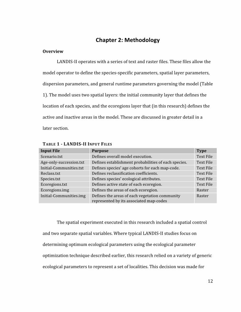
LANDIS-‐II operates with a series of text and raster files. These files allow the

model operator to define the species-‐specific parameters, spatial layer parameters,

dispersion parameters, and general runtime parameters governing the model (Table

1). The model uses two spatial layers: the initial community layer that defines the

location of each species, and the ecoregions layer that (in this research) defines the

active and inactive areas in the model. These are discussed in greater detail in a

later section.

TABLE 1 - LANDIS-II INPUT FILES Input File Purpose Type Scenario.txt Defines overall model execution. Text File Age-‐only-‐succession.txt Defines establishment probabilities of each species. Text File Initial-‐Communities.txt Defines species’ age cohorts for each map-‐code. Text File Reclass.txt Defines reclassification coefficients. Text File Species.txt Defines species’ ecological attributes. Text File Ecoregions.txt Defines active state of each ecoregion. Text File Ecoregions.img Defines the areas of each ecoregion. Raster Initial-‐Communities.img Defines the areas of each vegetation community

represented by its associated map-‐codes Raster

The spatial experiment executed in this research included a spatial control

and two separate spatial variables. Where typical LANDIS-‐II studies focus on

determining optimum ecological parameters using the ecological parameter

optimization technique described earlier, this research relied on a variety of generic

ecological parameters to represent a set of localities. This decision was made for

13

three reasons. First, it is a requirement of the concurrent research involving the

development of a vegetation trend database to process a broad range of ecological

parameters. Second, the experimental results using different ecological regimes only

serves to bolster the validity of the results because ecological parameters can

remain fixed. Third, ecological parameter sensitivity is not the focus of this research,

but rather the spatial properties of the underlying datasets. Therefore, any

ecological parameters could have been used in this study, provided they remained

constant between the experimental control and variables.

For this study, ecological regimes were defined as the set of dominant,

natural, terrestrial vegetation communities within the boundaries of a given locality.

The spatial control was defined as the spatial composition and arrangement of

vegetation communities at each locality. Each variable, at each locality, was

processed by LANDIS using thirty separate iterations of the model and the results

were aggregated for more robust comparison. The spatial control variable used the

same spatial input layer, but LANDIS’s random-‐seed value was changed. The

random-‐seed value governs the stochasticity of the model, such that running

LANDIS-‐II with the same set of input parameters, layers, and random-‐seed value

always produces the same result. To produce a range of results with the same input

parameters and layers, the random-‐seed value must change. Running a set of thirty

iterations of each variable at each locality in LANDIS-‐II was determined to

effectively capture the range of vegetation trend succession occurring for each

14

instance of each variable at each locality. This acknowledges Mlandenoff’s earlier

quote and provides a stable dataset to assess vegetation trends for each variable.

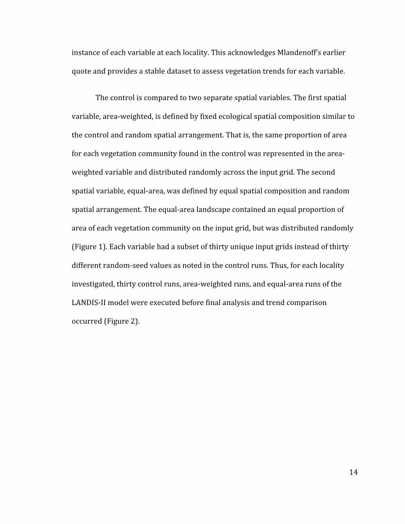
The control is compared to two separate spatial variables. The first spatial

variable, area-‐weighted, is defined by fixed ecological spatial composition similar to

the control and random spatial arrangement. That is, the same proportion of area

for each vegetation community found in the control was represented in the area-‐

weighted variable and distributed randomly across the input grid. The second

spatial variable, equal-‐area, was defined by equal spatial composition and random

spatial arrangement. The equal-‐area landscape contained an equal proportion of

area of each vegetation community on the input grid, but was distributed randomly

(Figure 1). Each variable had a subset of thirty unique input grids instead of thirty

different random-‐seed values as noted in the control runs. Thus, for each locality

investigated, thirty control runs, area-‐weighted runs, and equal-‐area runs of the

LANDIS-‐II model were executed before final analysis and trend comparison

occurred (Figure 2).

15

FIGURE 1– AN EXAMPLE OF THE EXPERIMENTAL VARIABLES AND ITERATIONS USED IN THIS RESEARCH

This figure diagrams the spatially explicit control and two spatial variables used to test the spatial sensitivity of LANDIS-‐II in this research. The control was iterated using a series of different random-‐seed values in LANDIS-‐II. The two variables were iterated by creating thirty different input grids.

16

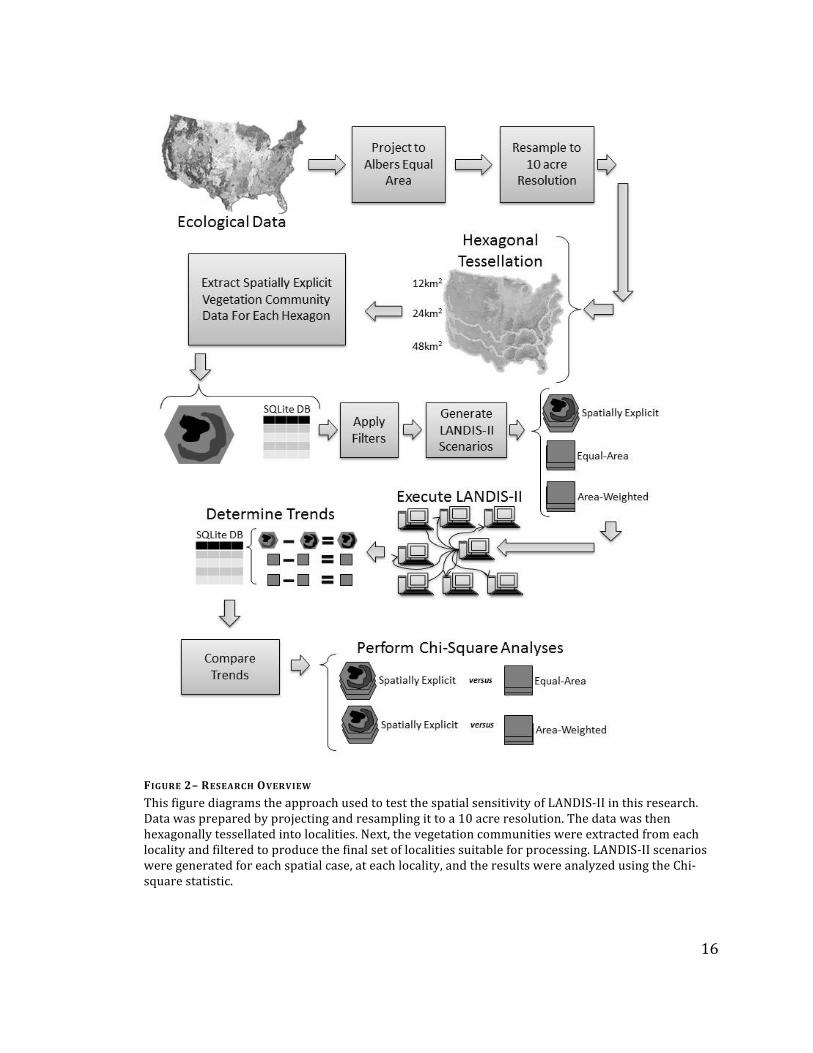
FIGURE 2– RESEARCH OVERVIEW

This figure diagrams the approach used to test the spatial sensitivity of LANDIS-‐II in this research. Data was prepared by projecting and resampling it to a 10 acre resolution. The data was then hexagonally tessellated into localities. Next, the vegetation communities were extracted from each locality and filtered to produce the final set of localities suitable for processing. LANDIS-‐II scenarios were generated for each spatial case, at each locality, and the results were analyzed using the Chi-‐square statistic.

17

The hypothesis of this research is that, significantly more often than not,

aspatial vegetation trends produced by LANDIS-‐II based on a spatially explicit input

control parameter (i.e. digital representation of the real environment) are similar to

trends generated using the area-‐weighted variable. Further, succession trends

generated using the equal-‐area variable produce trend results similar to the control

case significantly more often than not, but less often than the area-‐weighted case.

Each of these trend comparisons were assessed at three different scales to

determine the effect locality size has on each result (Figure 1).

Testing the stochasticity of the LANDIS-‐II model involves a significant

amount of computer resources and data handling. This research used the python

programming language and numerous site-‐packages. The site-‐package for SQLite

(SQLite3) was used to store large datasets that were easily queried. The NumPy and

SciPy site-‐packages were used to generate stochastic spatial arrangements and

perform the final analysis. Esri’s ArcPy was used to load, convert, and store a variety

of raster file formats. Finally, the Python language was instrumental in the

automation of LANDIS-‐II simulations. A simple client-‐server environment for

distributing the computing load across multiple machines was developed for this

project (Figure 1). Pseudo-‐code used to implement many of the more complex tasks

is available in the appendicies.

18

Vegetation Community Dataset

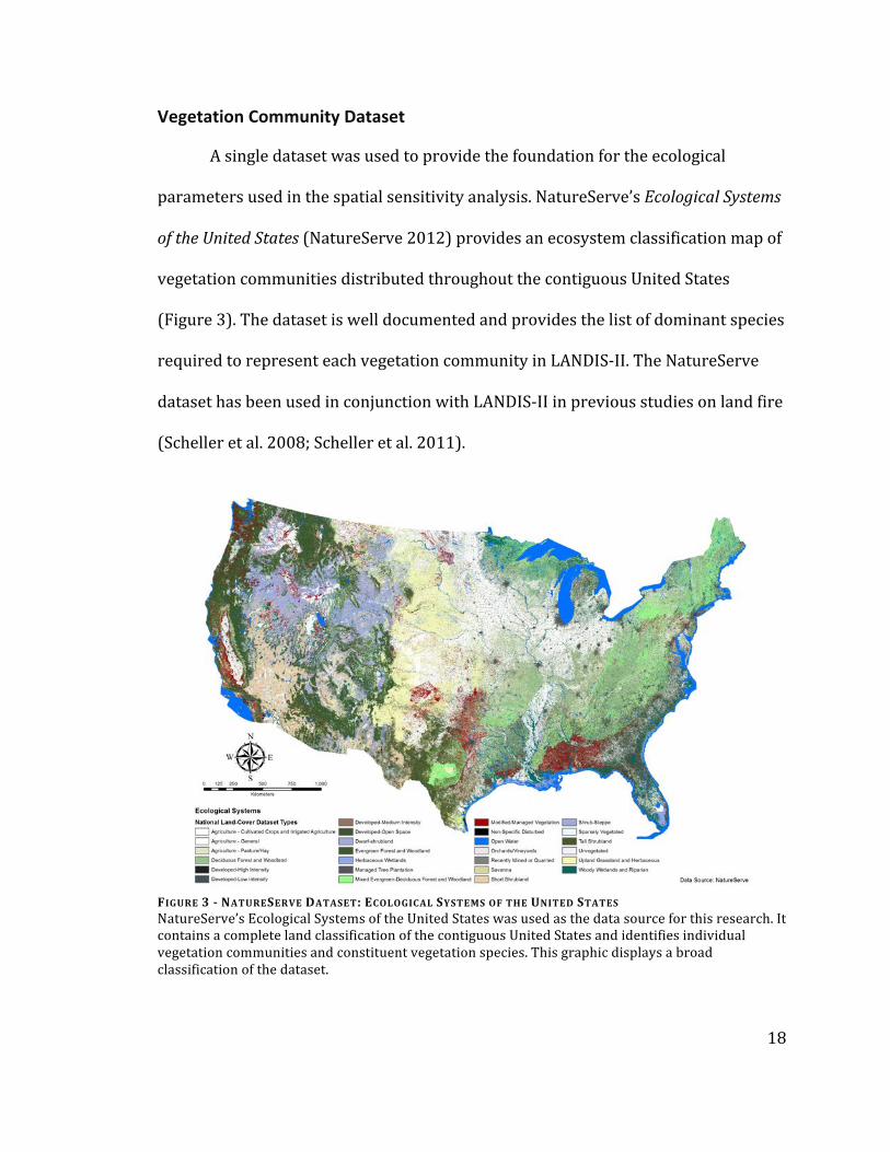
A single dataset was used to provide the foundation for the ecological

parameters used in the spatial sensitivity analysis. NatureServe’s Ecological Systems

of the United States (NatureServe 2012) provides an ecosystem classification map of

vegetation communities distributed throughout the contiguous United States

(Figure 3). The dataset is well documented and provides the list of dominant species

required to represent each vegetation community in LANDIS-‐II. The NatureServe

dataset has been used in conjunction with LANDIS-‐II in previous studies on land fire

(Scheller et al. 2008; Scheller et al. 2011).

FIGURE 3 - NATURESERVE DATASET: ECOLOGICAL SYSTEMS OF THE UNITED STATES NatureServe’s Ecological Systems of the United States was used as the data source for this research. It contains a complete land classification of the contiguous United States and identifies individual vegetation communities and constituent vegetation species. This graphic displays a broad classification of the dataset.

19

The NatureServe dataset was prepared for further processing by first

projecting it into the Albers Equal Area coordinate system (2012a) such that each

locality contained an equal number of raster cells. The concurrent research project

had a 10-‐acre minimum mapping area requirement (personal communication with

Dr. Eric Britzke); therefore, the NatureServe raster was resampled from a 30-‐m2

spatial resolution, to a 10-‐acre spatial resolution using a majority-‐area approach.

The resampling process reduced the computational intensity of this study by

limiting the time required to calculate each locality’s vegetation community regime.

It should be noted that the 10-‐acre resampling procedure slightly accentuates

dominant landscape communities, which was acceptable given the research

preference toward dominant communities.

Locality Dataset

The NatureServe dataset was tessellated into three continuous hexagonal

polygon shapefiles, where each individual polygon represents a candidate locality

suitable for investigation (e.g., Figure 4).

20

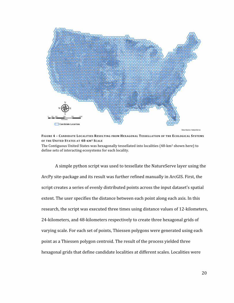
FIGURE 4 – CANDIDATE LOCALITIES RESULTING FROM HEXAGONAL TESSELLATION OF THE ECOLOGICAL SYSTEMS OF THE UNITED STATES AT 48-KM2 SCALE

The Contiguous United States was hexagonally tessellated into localities (48-‐km2 shown here) to define sets of interacting ecosystems for each locality.

A simple python script was used to tessellate the NatureServe layer using the

ArcPy site-‐package and its result was further refined manually in ArcGIS. First, the

script creates a series of evenly distributed points across the input dataset’s spatial

extent. The user specifies the distance between each point along each axis. In this

research, the script was executed three times using distance values of 12-‐kilometers,

24-‐kilometers, and 48-‐kilometers respectively to create three hexagonal grids of

varying scale. For each set of points, Thiessen polygons were generated using each

point as a Thiessen polygon centroid. The result of the process yielded three

hexagonal grids that define candidate localities at different scales. Localities were

21

considered “candidate” because a series of vegetation filters had not yet been

applied to select only those localities meeting a series of target criteria.

Building a Landscape Diversity Database

Before the set of candidate localities was filtered, the vegetation community

dataset needed to be configured in a rapidly queriable manner. For each locality, the

ArcGIS Extract By Mask tool (2012b) extracted the set of NatureServe community

values found within the hexagonal extent. The ArcPy RasterToNumPyArray (2013b)

function converted the extracted result into an array suitable for evaluation using

the NumPy Site-‐Package (2013a). The NumPy Unique function operated on the

returned array to produce the set of unique community values found in each

candidate locality under investigation. Each community value and its associated cell

count (or area in 10-‐acre units) was inserted into a SQLite table. If a locality was not

contained by the data extent of the NatureServe raster, it was ignored.

By using a SQLite table, filtering landscape classification data to determine

the final set of localities can be performed through the use of SQL queries rather

than slower more complicated raster based queries. The use of a table also allows

the researcher to retain a filter identifier that specifies the criteria used to remove a

particular locality from consideration.

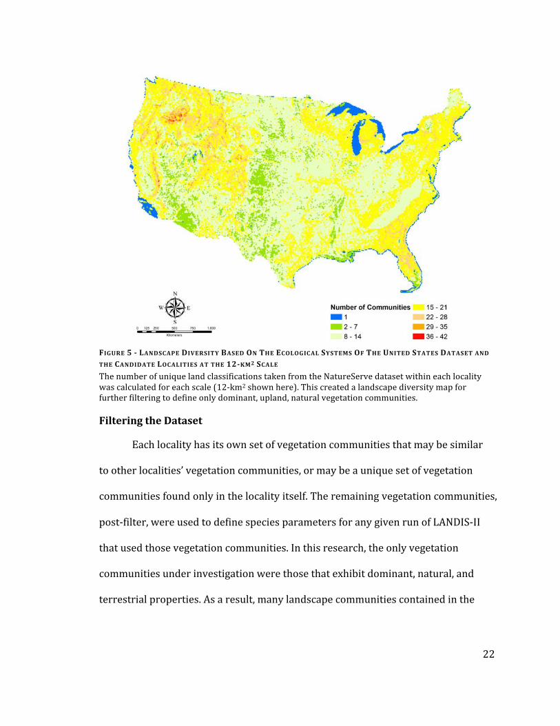
As byproduct of the research approach, by tallying the number of unique

communities in each locality, it was possible to create a landscape diversity map

(Figure 5).

22

FIGURE 5 - LANDSCAPE DIVERSITY BASED ON THE ECOLOGICAL SYSTEMS OF THE UNITED STATES DATASET AND THE CANDIDATE LOCALITIES AT THE 12-KM2 SCALE

The number of unique land classifications taken from the NatureServe dataset within each locality was calculated for each scale (12-‐km2 shown here). This created a landscape diversity map for further filtering to define only dominant, upland, natural vegetation communities.

Filtering the Dataset

Each locality has its own set of vegetation communities that may be similar

to other localities’ vegetation communities, or may be a unique set of vegetation

communities found only in the locality itself. The remaining vegetation communities,

post-‐filter, were used to define species parameters for any given run of LANDIS-‐II

that used those vegetation communities. In this research, the only vegetation

communities under investigation were those that exhibit dominant, natural, and

terrestrial properties. As a result, many landscape communities contained in the

23

NatureServe dataset were removed; including, agricultural lands, wetlands, barren

lands, and urban areas.

The first filter removed all landscape communities that did not represent

natural, terrestrial vegetation. Of the remaining landscape communities defined by

the NatureServe dataset, two were missing appropriate species information and

were removed.

The second filter focused on the composition of each candidate locality.

Recall that vegetation communities are the set of collocated species occurring on the

landscape as classified by NatureServe. For the given set of vegetation communities

contained by a candidate locality, the total area of each individual vegetation

community had to represent at least 3.34% of the total locality area. This minimum

area threshold was determined by calculating the total area of each vegetation

community in a locality, and dividing it by the total area of that locality, to determine

the proportional area of each vegetation community in each locality. The set of

proportional areas for all vegetation communities in all localities were binned into

thirty bins, where the first bin represented the smallest proportional areas found

across all localities. Thus, the first bin represented vegetation communities on the

local landscape considered to be non-‐dominant (i.e. a vegetation community

occupied less than 3.34% of the locality’s area). By removing the non-‐dominant

communities in each locality, only vegetation communities that were considered to

24

be dominant (the targets of this research) in those localities remained, regardless of

their patchiness on the landscape.

The third filter applied acted to limit the number of communities being

evaluated. If a candidate locality had more than six unique vegetation communities

remaining after the first two filters were applied, it was removed from

consideration. Conceptually, areas of real-‐world landscape that exhibit more than

six different dominant vegetation communities at a given locality are highly complex

and may be driven by ecological drivers other than vegetation dispersion; such as

elevation regime or soil patterns (personal communication, Dr. Eric Britzke). Seven

localities were removed as a result of this maximum threshold filter.

Also, since there must be more than one kind of vegetation community

represented in LANDIS to fuel succession, all localities containing only one kind of

community were removed from further consideration.

The final threshold applied to the dataset ensured that candidate localities

exhibited natural, terrestrial connectivity and that the locality was dominated by

natural systems. Candidate localities were removed from further processing if the

collective set of remaining communities under investigation occupied less than 60%

of the total area of the locality. The 60% threshold was used based on the

suggestions of percolation theory (Majewski and Malarz 2008). Percolation theory is

a branch of statistical physics that explains the probability of connectivity in a lattice.

25

The theory defines a set of percolation thresholds, that when met, predict the

existence of a single path between one side of a lattice and its opposing side, passing

only through cells of the same value; in this case, cells occupied by natural

vegetation.

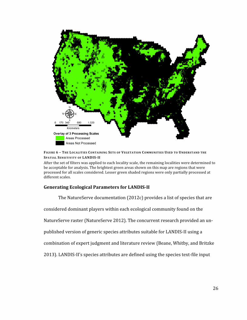
The final set of localities used in this research were concentrated in New

England, the Appalachian Mountains, scattered areas in the Midwest, and much of

the public land-‐dominated regions of the Intermountain West, and open spaces of

the West Coast. Areas not included were the large expanses of agriculture and

silvicuture in the Midwest and Southeast, and the large wetland ecosystems of the

Gulf Coastal Plain and Florida (Figure 6).

26

FIGURE 6 – THE LOCALITIES CONTAINING SETS OF VEGETATION COMMUNITIES USED TO UNDERSTAND THE SPATIAL SENSITIVITY OF LANDIS-II

After the set of filters was applied to each locality scale, the remaining localities were determined to be acceptable for analysis. The brightest green areas shown on this map are regions that were processed for all scales considered. Lesser green shaded regions were only partially processed at different scales.

Generating Ecological Parameters for LANDIS-II

The NatureServe documentation (2012c) provides a list of species that are

considered dominant players within each ecological community found on the

NatureServe raster (NatureServe 2012). The concurrent research provided an un-‐

published version of generic species attributes suitable for LANDIS-‐II using a

combination of expert judgment and literature review (Beane, Whitby, and Britzke

2013). LANDIS-‐II’s species attributes are defined using the species text-‐file input

27

parameter and govern each species’ behavior at runtime (Scheller and Domingo

2011).

LANDIS-‐II’s initial communities input layer is a raster file (e.g. *.img, *.gis)

that defines the spatial arrangement and distribution of vegetation communities

(Scheller and Domingo 2011). Each cell of the initial communities input raster may

contain multiple species of varying ages based on the parameters found in the initial

communities text file. In this research, these communities were identified for

localities within the contiguous United States; where each locality exhibited a given

set of vegetation communities. While the generation of initial community input

layers is discussed in a latter section, its associated map-‐codes are discussed here.

Vegetation communities in natural systems are composed of species at

different stages of their lifecycles (Watt 1947). To capture age diversity in the real

landscape, vegetation communities were parsed into different map-‐codes by the

researcher to allow species age variability to be appropriately modeled in LANDIS-‐II.

For each vegetation community, a set of twelve map-‐codes was assigned with

different age distributions to better represent the range of vegetation community

age structures found on the landscape. The age distributions were based on the

longevity of each constituent species. Each map-‐code represents an equal

proportion of the area each vegetation community represents in a given spatial

variable or control. The use of a longevity-‐based metric was chosen over a sexual-‐

28

maturity based metric because the forestry profession has a better understanding of

a given species longevity over a species’ sexual maturity.

The distribution of input species age was set at 80%, 50%, 30%, and 10% of

each species’ longevity. In LANDIS-‐II, species begin to die after their age was greater

than 80% of that species’ longevity. This age class was used to represent vegetation

communities at the end of their lifecycles. The 50% and 30% of longevity age classes

were used to represent two different mid-‐growth stages. The 10% of longevity age

class was used to represent a community early in its lifecycle.

In the first four, out of twelve, map-‐codes, species ages were assigned as 80%,

50%, 30%, or 10% of each species’ longevity to create four homogenously aged

cohorts. The next four map-‐codes assigned sets of age classes to each species to

create map-‐codes with mixed ages. The sets were: 80% and 50%; 80% and 30%;

10% and 30%; and 80%, 50%, 30%, and 10%. The remaining four map-‐codes

randomly assigned species ages, or sets of ages, taken from the first eight map-‐codes.

Map-‐code generation was repeated for each vegetation community at each locality

under investigation. Multiple species with varying ages can occur in each cell of the

raster used to represent a spatial variable or the experimental control to comprise a

vegetation community.

LANDIS-‐II uses establishment probabilities to determine the likelihood that a

particular species will establish itself in a new location after dispersal (Scheller and

29

Domingo 2011). Often these values are optimized for extremely site-‐specific studies

using the ecological parameter optimization process discussed earlier to take into

account soil and climatic conditions. Because this research tested LANDIS-‐II’s spatial

sensitivity at thousands of different sites, all establishment probabilities were set to

0.6 (on a 0 to 1.0 scale). This ensured all species are more likely than not to establish

themselves at new locations and that succession was more likely than not to occur.

Further, by fixing the establishment probability for all species, at all localities, allows

for a clearer picture of the spatial sensitivity of the model to be produced.

The LANDIS-‐II ecoregion layer parameter allows the user to define different

sets of establishment probabilities for different locations on the initial communities

input layer. It also allows certain areas of the map to be considered inactive in the

model (Scheller and Domingo 2011). For the purposes of this research, areas of the

initial communities layer containing vegetation communities under investigation

were part of the “alive” region. Areas of the initial communities layer containing

land classification values not under investigation (those areas removed by the filter)

were considered part of the “dead” region. The “dead” region was set to be inactive

in the model. Once again, to simplify the ecological parameters and focus on the

spatial sensitivity of LANDIS-‐II the ecoregion parameter was effectively rendered

homogenous for each locality regardless of soil and microclimate.

The final ecological parameter defined by this research was each species’

reclassification coefficient. Reclassification coefficients allow LANDIS-‐II to

30

determine which vegetation community a given cell should belong to on the initial

communities layer, based on the set of species occurring at that location. In this

research the succession trajectory of vegetation communities and not species was

assessed. In LANDIS-‐II vegetation communities are represented by their constituent

species, therefore, vegetation communities must be parameterized as a collection of

species in LANDIS-‐II. After the model disperses each vegetation community’s

constituent species, its initial community layer must be reclassified to determine the

new locations and areas where each vegetation community resides. If all species are

given equivalent reclassification values for each community, then communities have

an equal chance of being assigned to a cell if those communities happen to contain

the same species, and a species generally used for community discrimination is not

present (Scheller and Domingo 2011). All reclassification values for this study were

equal in value (set to 0.5 on a 0 to 1.0 scale).

LANDIS-‐II’s reclassification calculation also considers species age as a

proportion of its longevity. Older species on the landscape are given higher

reclassification values in LANDIS-‐II by default. By structuring the parameter as

described above, a vegetation community must complete its ecological succession

before it is reclassified to a new community.

Extracting Spatially Explicit Rasters

The spatially explicit rasters required for the experimental control were

extracted using a python script that iteratively selected a given locality hexagon,

31

extracted values from the NatureServe dataset using the Extract By Mask tool and

classified the resulting layer using the NumPy site-‐package. The classification

scheme used divides each vegetation community area into twelve zones, one for

each map-‐code, to represent the age mixes of each species in the vegetation

community in LANDIS-‐II. The map-‐code values were recycled between runs

representing different localities with different sets of vegetation communities.

Regions of the grid that were missing vegetation community values, or exhibited

community values that were filtered out, were given a value of zero and defined as

inactive areas using the ecoregion parameter layer in LANDIS-‐II. The spatially

explicit layer was processed in LANDIS-‐II using different random-‐seed values for

each run to capture the spatial variation of model results. Every extracted raster

was stored in its own uniquely named folder.

Generating Random Rasters

The area-‐weighted spatial variable maintains the proportion of area each

ecological community represents in a locality. The ecological community

composition was extracted from the SQLite database created during the initial phase

of this research. The spatial arrangement was generated randomly using the NumPy

Random Choice function of the NumPy site-‐package. The total number of cells on the

input raster was equivalent to the number of cells contained in the total area of a

given locality. Thirty different area-‐weighted spatial scenarios were generated for

each locality to provide a range of inputs into the model.

32

The equal-‐area variable represents equal areas of vegetation communities in

a locality with random spatial arrangement. This dataset was generated in a similar

fashion to the area-‐weighted rasters; the exception being, post-‐filter vegetation

communities were given an equivalent amount of area on the generated raster.

Thirty equal-‐area spatial scenarios were generated for each locality as well. Every

random grid generated was stored in its own uniquely named folder.

Building LANDIS-II Input Text-Files

LANDIS-‐II is operated using a series of text-‐files. The LANDIS-‐II text-‐files

used as input and parameter files were generated for each uniquely named folder

containing an input raster (Table 1). These text-‐files were generated using object-‐

oriented python code that represented each text-‐file as a different method within a

LandisInput class. The class parsed a dictionary of model variables for each input

file passed to the script as input arguments. Then a Create method was called that

generated all of the input text-‐files and saved each set of text-‐files to its associated

uniquely named folder, containing its initial communities input raster.

An ecoregion raster was generated for each initial communities raster by

assigning a value of one to each cell that was not equal to zero. Each initial

communities raster file was read-‐in using the ArcPy site-‐package. It was then

converted to a NumPy array for further processing. Once the array was classified as

one or zero it was saved as a different filename. This created the spatial parameter

33

that defined the active or inactive state of certain areas in the model (i.e. the

ecoregion parameter layer).

The model scenario was further established such that the time-‐step for

succession in the model occurred every 3-‐years. The temporal duration of the

scenario was set to 80-‐years to match the time horizon of the concurrent research

project. The Age Reclass Output Extension time-‐step was set to 40-‐years such that

the model output initial-‐state, mid-‐state, and end-‐state output.

Executing LANDIS-II

The large number of LANDIS-‐II runs required development of simple server

and client scripts in python to distribute the processing load across multiple

computers. First, all of the folders containing LANDIS-‐II input files were copied to a

network drive that all computers had access to. Because each folder represents a

different run of LANDIS-‐II, the server script built the list of required LANDIS-‐II runs

by populating a list of folders on the network file-‐share. Next, the server script

extended python’s SocketServer site-‐package and overrode the handle method to

handle each request made to the server. When a client computer signaled it was

ready to process a LANDIS-‐II run, the server sent a filename of a given folder on the

network share. The client copied the folder to the local machine, executed the

LANDIS-‐II run and copied the results back to the network file-‐share.

The client was also able to execute multiple runs of LANDIS-‐II simultaneously

by using python’s multiprocessing site-‐package. A pool of workers was defined such

34

that each worker downloaded a LANDIS-‐II run and executed it in a sub-‐process. This

allowed the client to take advantage of the multi-‐core processors found on each

computer. For any given scenario of the LANDIS-‐II model, the average execution

time was approximately 4 seconds. The processing of all runs took nearly 200 hours

on eleven different machines.

The server and client code is shown in the Appendicies A and B.

Developing Vegetation Trends

The spatially explicit control case was represented as a hexagon due to the

tessellation method used. The spatial variables were represented as square rasters

to reduce computational complexity during variable generation. The shape of the

spatial variables is considered irrelevant because each was constructed randomly

based on a proportional representation of ecological communities. As an example,

consider a locality occupied by two habitats; Mediterranean California Lower

Montane Black Oak-‐Conifer Forest and Woodland, and North Pacific Dry Douglas-‐fir-‐

(Madrone) Forest and Woodland (Figure 7). This research demonstrated a slight

increase in the Mediterranean California Lower Montane Black Oak-‐Conifer Forest

and Woodland habitat in each spatial variable. By examining the proportional

representation of landscape succession trends in each spatial variable and

comparing it to the proportional representation of trends in the spatial control, it is

possible to demonstrate that the trends are similar.

35

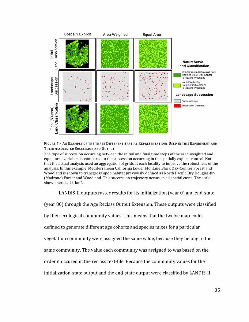
FIGURE 7 – AN EXAMPLE OF THE THREE DIFFERENT SPATIAL REPRESENTATIONS USED IN THIS EXPERIMENT AND THEIR ASSOCIATED SUCCESSION AND OUTPUT

The type of succession occurring between the initial and final time steps of the area-‐weighted and equal-‐area variables is compared to the succession occurring in the spatially explicit control. Note that the actual analysis used an aggregation of grids at each locality to improve the robustness of the analysis. In this example, Mediterranean California Lower Montane Black Oak-‐Conifer Forest and Woodland is shown to transgress upon habitat previously defined as North Pacific Dry Douglas-‐fir-‐(Madrone) Forest and Woodland. This succession trajectory occurs in all spatial cases. The scale shown here is 12-‐km2.

LANDIS-‐II outputs raster results for its initialization (year 0) and end-‐state

(year 80) through the Age Reclass Output Extension. These outputs were classified

by their ecological community values. This means that the twelve map-‐codes

defined to generate different age cohorts and species mixes for a particular

vegetation community were assigned the same value, because they belong to the

same community. The value each community was assigned to was based on the

order it occured in the reclass text-‐file. Because the community values for the

initialization-‐state output and the end-‐state output were classified by LANDIS-‐II

36

using the same method, the comparison between the two layers produced the

switching trend for each LANDIS-‐II run.

Because the maximum number of communities that could occur on an output

raster is six due to the initial filtering procedure, the values on the output raster

were always less than or equal to six. The initialization-‐state raster was multiplied

by ten and added to the end-‐state raster. A python script cast each raster to a

NumPy array to complete this process.

The result produced an array of values, where the first digit of each value

represents the initial state and the second digit of each value represents the final

state. Values that are zero represent inactive areas of the grid. Values that are

cleanly divisible by ten (e.g., 10, 20, 30) represent areas where all species

experienced a die-‐off, and succession has yet to occur. This comparison was

completed for every set of LANDIS-‐II output. In these experiments, ecological

disturbances were not modeled. Isolated incidences of a few cells experiencing a

die-‐off due to a species reaching its maximum age may occur; but in reality, discrete

ecological transitions are rarely seen in undisturbed environments and were an

artifact of the model’s representation of ecological processes.

The result of each comparison was compiled in a SQLite table. The

comparison table used scale, locality, run-‐type, and iteration fields to uniquely

describe each run. Values for the scale column (i.e., 12, 24, and 48) were associated

37

to the spatial extent of each model run. The locality column stored the feature

identifier of the associated initial input locality. The run-‐type field described

whether or not the run was spatially explicit, area-‐weighted, or equal-‐area. The

iteration column held a value that noted which iteration the run represented (i.e. 1

through 30). The table also included a column for the initial vegetation community

values, final vegetation community values, and the area of each change between an

initial and final vegetation community pair. These changes represent the landscape

succession.

By storing the comparison data in a SQLite table, it is possible to perform

rapid queries for each unique set of runs. Each experimental variable and the

control were comprised of thirty individual runs to form an aggregate assessment of

vegetation trends. Aggregates were made for each combination of scale, locality, and

run-‐type. To generate the aggregate vegetation community succession trend, each

succession trend’s area was summed for all thirty runs and stored in an aggregation

table; such that, the original and final fields in the aggregation table represented the

total number of cells transitioning from the initial vegetation community to the final

vegetation community across all thirty iterations. An analysis of these trends

yielded the evidence necessary to partially accept and reject the research

hypotheses.

38

Statistical Testing

Through the use of the SQLite and SciPy python site-‐packages it was possible

to perform a Chi-‐square analysis at each locality using the experimental control as

the expected value and each experimental variable as separate observed cases. The

SQLite table containing the aggregated values of vegetation community trends for

each locality supplied the input data for the Chi-‐square analyses.

Three categories of Chi-‐square analysis were used to compare the

experimental control to the experimental variables. The first analysis focused on the

succession trajectory of the landscape by assessing each trend as a proportion of its

initial starting area. The second Chi-‐square analysis considered the succession

trajectory of each trend as a proportion of the total landscape area. The final Chi-‐

square analysis evaluated the model end-‐states for each trend to determine the

overall sensitivity of the model using the end-‐state proportion of each vegetation

community out of the total area.

By comparing proportions instead of actual cell counts it was possible to

ignore inactive areas in the spatially explicit experimental control and focus only on

the aspect of the landscape that was of interest.

For the first Chi-‐square analysis at a given locality, the degrees of freedom

were defined as the total number of succession trends occurring across all spatial

cases (spatially explicit, area-‐weighted, equal-‐area) at a particular scale, minus one.

Next, the total area of the input vegetation community at its initial state divided the

39

area represented by each trend. The trends generated using spatially explicit input

were compared to the trends produced in the area-‐weighted variable, and

separately the equal-‐area variable using the Chi-‐square formula (Figure 8). This

analysis was carried out by querying the SQLite table of aggregated data in Python,

calculating the degrees of freedom and the Chi-‐square statistic, and using SciPy to

determine each statistic’s associated alpha value. The results of the comparisons

were stored in a SQLite table and represented the trajectory of landscape change as

a proportion of each vegetation community’s initial state.

FIGURE 8 - CHI-SQUARE EQUATION

The Chi-‐square equation was used to determine the trends produced when the experimental control (i.e. spatially explicit case) was compared to the two experimental variables; area-‐weighted and equal-‐area.

The second analysis was similar to the first, except that instead of calculating

the initial area proportions as a percentage of each vegetation community’s initial

state, the calculation represents the area proportion of the succession trend to the

total area of the active grid. The degrees of freedom were still defined by the

number of succession trends across all runs at a given locality. The results of this

analysis were stored in a separate SQLite table and represented the trajectory of

succession of each vegetation community as a proportion of the total area of the grid.

The final analysis compared the experimental control and variables at the

output end-‐state to determine the amount of equifinality that occurred in the results.

40

The aggregated data for each locality was extracted from the SQLite table. The

proportion each vegetation community represented as a ratio to the total active area

of the grid at the model’s end-‐state was calculated. This calculation was made by

summing the areas of each vegetation community using the SQL SUM function and

the GROUP BY aggregator; these sums were further divided by the total area of the

active grid. The degrees of freedom were defined by the total number of unique

vegetation communities occurring at the end-‐state minus one. Next, the Chi-‐square

statistic was calculated between the spatially explicit experimental control and each

variable and the result was stored in a new SQLite table.

The python pseudocode used to implement these analyses may be found in

Appendix C.

41

Chapter 3: Results

Recall that the first test used the Chi-‐square statistic to determine the

similarity between the spatially explicit case and the two spatial variables

individually. The analysis focused on the succession trajectories as a proportion of

each vegetation community’s initial area. This analysis was completed at every

locality under investigation at each scale. At the 95% confidence level, there is less

than 1% difference between the comparisons of each spatial variable to the spatial

control at any given scale; but, there is approximately a 10% difference between the

results at each scale. The results also indicate that a dataset containing random

spatial arrangements and percentage-‐area compositions can substitute for spatially

explicit data between 40% and 60%, or on average half, of the time. The full range of

confidence levels for the chi-‐square analysis was calculated due to the requirements

of the concurrent research. The full range is shown here to indicate a slightly

decreasing number of runs considered to be different from the control at increasing

levels of confidence (Figure 9).

42

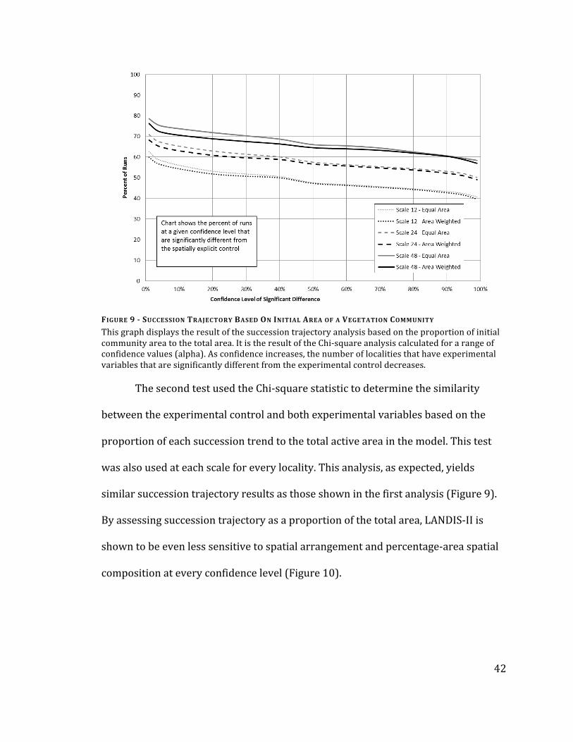
FIGURE 9 - SUCCESSION TRAJECTORY BASED ON INITIAL AREA OF A VEGETATION COMMUNITY

This graph displays the result of the succession trajectory analysis based on the proportion of initial community area to the total area. It is the result of the Chi-‐square analysis calculated for a range of confidence values (alpha). As confidence increases, the number of localities that have experimental variables that are significantly different from the experimental control decreases.

The second test used the Chi-‐square statistic to determine the similarity

between the experimental control and both experimental variables based on the

proportion of each succession trend to the total active area in the model. This test

was also used at each scale for every locality. This analysis, as expected, yields

similar succession trajectory results as those shown in the first analysis (Figure 9).

By assessing succession trajectory as a proportion of the total area, LANDIS-‐II is

shown to be even less sensitive to spatial arrangement and percentage-‐area spatial

composition at every confidence level (Figure 10).

43

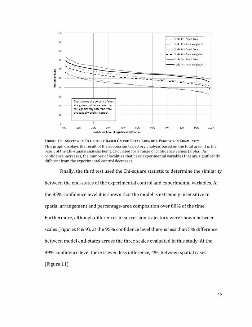
FIGURE 10 - SUCCESSION TRAJECTORY BASED ON THE TOTAL AREA OF A VEGETATION COMMUNITY

This graph displays the result of the succession trajectory analysis based on the total area. It is the result of the Chi-‐square analysis being calculated for a range of confidence values (alpha). As confidence increases, the number of localities that have experimental variables that are significantly different from the experimental control decreases.

Finally, the third test used the Chi-‐square statistic to determine the similarity

between the end-‐states of the experimental control and experimental variables. At

the 95% confidence level it is shown that the model is extremely insensitive to

spatial arrangement and percentage-‐area composition over 80% of the time.

Furthermore, although differences in succession trajectory were shown between

scales (Figures 8 & 9), at the 95% confidence level there is less than 5% difference

between model end-‐states across the three scales evaluated in this study. At the

99% confidence level there is even less difference, 4%, between spatial cases

(Figure 11).

44

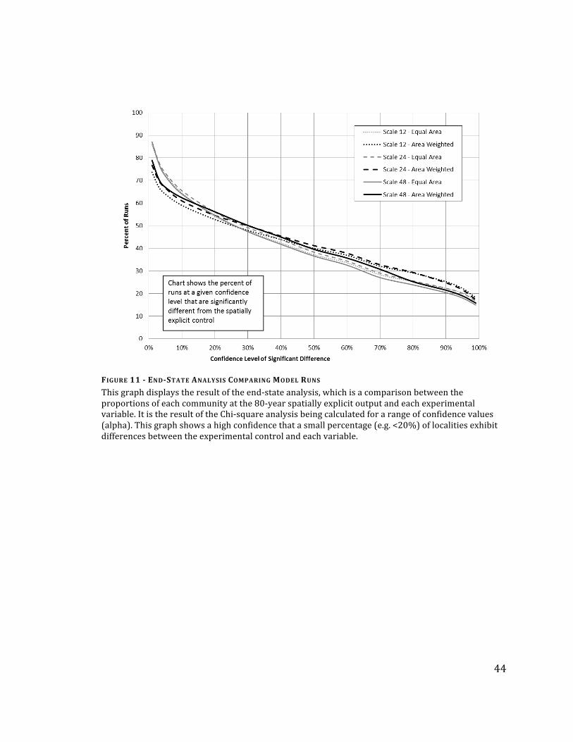
FIGURE 11 - END-STATE ANALYSIS COMPARING MODEL RUNS

This graph displays the result of the end-‐state analysis, which is a comparison between the proportions of each community at the 80-‐year spatially explicit output and each experimental variable. It is the result of the Chi-‐square analysis being calculated for a range of confidence values (alpha). This graph shows a high confidence that a small percentage (e.g. <20%) of localities exhibit differences between the experimental control and each variable.

45

Chapter 4: Discussion and Conclusion

Discussion

A review of the literature on the LANDIS-‐II model’s use and application

suggests that the spatial sensitivity of the model has largely been untested. Although

the current research does not test every possible avenue of spatial and ecological

parameterization of the LANDIS-‐II model, the spatial sensitivity of the model’s

fundamental spatial function (i.e. dispersion) has been assessed for a range of

spatial and ecological settings to understand the processes acting within the model’s

proprietary core. The results suggest that LANDIS-‐II is a spatially insensitive model

for determining vegetation succession trends. While the model does produce a

spatial output layer, the developer and user communities both consider it to be an

imaginary representation of reality, rather than an accurate prediction of a future

end-‐state (Mladenoff and He 1999).

The results do have two important caveats. On further review of the

underlying LANDIS-‐II runs where the Chi-‐square statistic returned a value of zero, it

appears that localities exhibiting only grass communities experience a complete die-‐

off in the model. Although not scientifically sound, it occurs in all spatial cases. By

slightly adjusting the grass species parameters to have maximum dispersion

distances greater than half the cell-‐size (i.e. >100m) dispersion occurs and species

die-‐off no longer happens. Also, due to longevity values less than 80 years (the time

horizon of this analysis) it appears that the grass longevity parameter does not

46

allow the grass species to survive in an undisturbed environment (one of the

assumptions in this study). While this caveat points to a flaw in the generic species

attributes used to model grass species in this research, since the same response

occurs for all spatial cases, the model can be shown to be spatially insensitive in

these instances. As such, the result is still valuable to this analysis.

The second caveat is the special case that occurs when the expected area of a

succession trend is zero and the observed succession trend area is greater than zero.

This special case was handled by adding a value of one to the expected and observed

values when performing the Chi-‐square evaluation. The squared difference between

the adjusted-‐expected and adjusted-‐observed value in the Chi-‐square statistic was

divided by the adjusted-‐expected value (one). This simplified the formula to be the

square of the original observed value. This case “explodes” the Chi-‐square results

and inflated the perceived differences between the spatial control and each spatial

variable. Thus, differences shown in the results are artificially inflated as a direct

result of the analytical mechanism used (i.e. the Chi-‐square statistic) and model

output is more similar than these results suggest. The Chi-‐square statistic was

chosen based on its low computational intensity and its ability to compare sets of

categories. Although the use of Chi-‐square is shown to affect the results, this is

acceptable because the elimination of the inflated values would only serve to

strengthen trends produced.

47

The results of this study indicate that succession trajectories between the

experimental control and both variables are likely to increase in difference as scale

increases. This is consistent with expectation because dispersion distance

parameters for any given species cover a larger proportion of the small 12-‐km2 grid

than the larger 24-‐km2 grid. Further, the differences in succession trajectory are

directly related to scale as a proportion of the total active area, and as a proportion

of the initial area of each vegetation community.

Although the succession trends seem to indicate reduced similarity as scale

increases, the end-‐state analysis suggests that the end-‐states are very similar

regardless of how the underlying changes are occurring. This would suggest that

there is some degree of equifinality occurring in the model. The differences between

the area-‐weighted results and the equal-‐area results are very small, less than 1% at

the 99% confidence level for differences between runs. This end-‐state metric is

considered to be more important because the proportion of vegetation communities

occurring at the end-‐state condition is typically used to document succession trends.

In acknowledging the research results, it appears that spatial arrangement

and percentage-‐area composition are not a requirement of the successful use of

LANDIS-‐II approximately 80% of the time at the 95% confidence level, provided the

ecological communities are known. These results represent a conservative estimate,

because of the artificial inflation of the Chi-‐square statistic discussed earlier. Stated

differently, the Chi-‐square null hypothesis that the experimental control is the same

48

as an experimental variable was rejected roughly 20% of the time with 95%

confidence.

The size of a given study area, however, is directly related to the method of

succession trajectory the vegetation communities undergo. The results of the first

two analyses (Figures 8 & 9) demonstrate that as processing area increases, the

difference between succession trajectories in the experimental variables and the

spatial control increase as well. Therefore, as the size of a study area increases,

succession may occur differently at different scales but the final end-‐state results

will be similar.

Conclusion This research assessed the spatial sensitivity of the LANDIS-‐II model to

spatial arrangement and spatial composition in homogenous spatial settings (the

LANDIS-‐II basic assumptions). No effort was taken to capture microclimate, solar

angle, elevation, or soils using variable establishment probabilities and ecoregions

to ensure all ecological parameters in the model remain fixed. The research

approach used the aggregate of thirty runs for the experimental control and each

experimental variable. Further, thousands of different localities were assessed with

different generically parameterized dominant, upland vegetation communities.

Although the results of this research point to caveats in the generalization of

ecological parameters, to understand the spatial sensitivity of the model in a

simplified environment optimum ecological parameters were not needed.

49

The first hypothesis of this research states that aspatial end-‐state vegetation

community succession trends based on spatially explicit parameters are similar to

results produced by parameters that maintain ecological composition but possess

random arrangement. Given the result of the end-‐state Chi-‐square analysis, this

hypothesis may be accepted. The second hypothesis of this research states that

aspatial end-‐state vegetation community succession trends based on spatially

explicit parameters are similar to results produced by parameters that do not

maintain ecological composition or arrangement, but exhibit less comparison than

the area-‐weighted case. The second hypothesis is accepted and rejected in part.

The equal-‐area variable did produce end-‐state results similar to that of the

spatially explicit control and in this sense the second hypothesis is accepted in part.

The equal-‐area variable, however, was not shown definitively to be more similar to

the control case than the area-‐weighted variable, therefore the second hypothesis is

rejected in part.

In conclusion, this research suggests that the spatial composition and

arrangement of an input layer into the LANDIS-‐II model may not be as important as

originally thought. These results suggest that LANDIS-‐II could be used to model

areas where spatially explicit information is poorly known, or in cases where

producing spatially explicit information is cost prohibitive. It is suggested that

future LANDIS-‐II studies assess the spatial sensitivity of their results when using

less generic ecological parameters. Future spatial tests of LANDIS-‐II could also be

50

done to determine the effects of spatial arrangement and composition when

microclimate or soils are defined by ecoregions and variable establishment

probabilities are used in the model. Finally, successive studies may also see value in

assessing spatial sensitivity for longer time durations and different scales than used

in this research.

51

References

Albers equal area conic. in Esri Inc. [database online]. 2012a [cited May 2013]. Available from http://resources.arcgis.com/en/help/main/10.1/index.html#/Albers_Equal_Area_Conic/003r0000001n000000/.

Extract by mask [database online]. 2012b [cited May 2013]. Available from

http://resources.arcgis.com/en/help/main/10.1/index.html#//009z0000002n000000. Esri Inc

He, H. S., D. R. Larsen, and D. J. Mladenoff. 2002. Exploring component-‐based

approaches in forest landscape modeling. Environmental Modelling & Software 17 (6): 519–529.

LANDIS-‐II User Community, "Moderated Discussion: Scaling Up LANDIS Results for

Regional Inference" (LANDIS-‐II Users Discussion, LANDIS-‐II, 2012). Legendre, Pierre, and Marie-‐Josree Fortin. 1989. Spatial pattern and ecological

analysis. Vegetatio 80 (2): 107–138. Majewski, Mariusz, and Krzysztof Malarz. 2008. Square latice site percolation

thresholds for complex neighborhoods. Krakow, Poland: AGH University of Science and Technology.

Mladenoff, David J., and Hong S. He. 1999. Design, behavior and application of

LANDIS, an object-‐oriented model of forest landscape disturbance and succession. In Spatial modeling of forest landscape change: Approaches and applications., eds. David J. Mladenoff, William L. Baker, 125–162. Cambridge, U.K.: Cambridge University Press.

Mladenoff, David J., George E. Host, Joel Boeder, and Thomas R. Crow. 1996. Landis:

A spatial model of forest landscape disturbance, succession, and management. In GIS and environmental modeling: Progress and research issues., eds. Michael F. Goodchild, Louis T. Steyaert, Bradley O. Parks, Carol Johnston, David Maidment, Michael Crane and Sandi Glendinning, 175–179. GIS World Books.

Morris, Andrew J. 1997. Representing spatial interactions in simple ecological

models. University of Warwick.

52

Nathan Beane, Michael Whitby and Eric Britzke, "Species Attributes" (Dataset, US Army ERDC, 2013), https://docs.google.com/file/d/0B4stw1Lkj0-‐dVXo2NTdUdk1WeGM/edit?usp=sharing.

NatureServe. NatureServe explorer. in NatureServe [database online]. 2012 [cited

March/2 2013]. Available from http://www.natureserve.org/explorer/. NatureServe explorer. in NatureServe [database online]. 2012c [cited May 2013].

Available from http://www.natureserve.org/explorer/servlet/NatureServe?init=Ecol.

NumPy reference. in The SciPy Community [database online]. 2013a [cited May

2013]. Available from http://docs.scipy.org/doc/numpy/reference/. Paine, Robert T., Mia J. Tegner, and Edward A. Johnson. 1998. Compounded

perturbations yield ecological surprises. Ecosystems 1 (6) : 535–545. Pultar, Edward, Martin Raubal, Thomas J. Cova, and Michael F. Goodchild. 2009.

Dynamic GIS case studies: Wildfire evacuation and volunteered geographic information. Transactions in GIS 13 : 85–104.

Raster to NumPy array. in Esri Inc. [database online]. 2013b [cited May 2013].

Available from http://resources.arcgis.com/en/help/main/10.1/index.html#//018v00000023000000.

Scheller, Robert M., and James B. Domingo. 2011. LANDIS-II model v6.0 user guide. Scheller, Robert M., James B. Domingo, Brian R. Sturtevant, Jeremy S. Williams,

Arnold Rudy, Eric J. Gustafson, and David J. Mladenoff. 2007. Design, development, and application of LANDIS-‐II, a spatial landscape simulation model with flexible temporal and spatial resolution. Ecological Modelling 201 (3–4) : 409–419.

Scheller, Robert M., and David J. Mladenoff. 2005. A spatially interactive simulation

of climate change, harvesting, wind, and tree species migration and projected changes to forest composition and biomass in northern Wisconsin, USA. Global Change Biology 11 (2): 307–321.

Scheller, Robert M., Steve Van Tuyl, Kenneth L. Clark, John Hom, and Inga La Puma.

2011. Carbon sequestration in the new jersey pine barrens under different scenarios of fire management. Ecosystems 14 (6): 987–1004.

53

Scheller, Robert M., Steve Van Tuyl, Kenneth Clark, Nicholas G. Hayden, John Hom, and David J. Mladenoff. 2008. Simulation of forest change in the new jersey pine barrens under current and pre-‐colonial conditions. Forest Ecology and Management 255 (5–6) : 1489–1500.

Shang, Bo Z., Hong S. He, Thomas R. Crow, and Stephen R. Shifley. 2004. Fuel load

reductions and fire risk in central hardwood forests of the united states: A spatial simulation study. Ecological Modelling 180 (1) : 89–102.

Tansley, A. G. 1935. The use and abuse of vegetational concepts and terms. Ecology

16 (3) : 284–307, Turner, Monica Goigel. 1989. Landscape ecology: The effect of pattern on process.

Annual Review of Ecology and Systematics 20 : 171–197. Watt, Alex S. 1947. Pattern and process in the plant community. Journal of Ecology

35 (1/2) : 1–22.

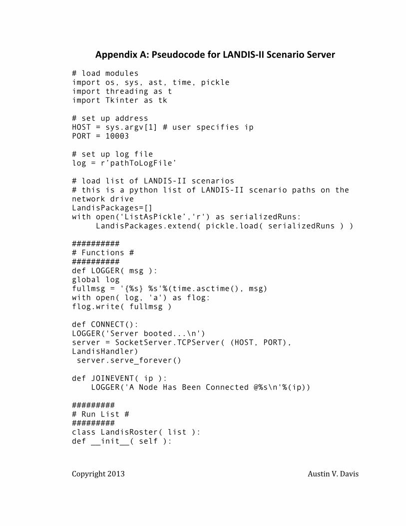
Copyright 2013 Austin V. Davis

Appendix A: Pseudocode for LANDIS-‐II Scenario Server

# load modules import os, sys, ast, time, pickle import threading as t import Tkinter as tk # set up address HOST = sys.argv[1] # user specifies ip PORT = 10003 # set up log file log = r’pathToLogFile’ # load list of LANDIS-II scenarios # this is a python list of LANDIS-II scenario paths on the network drive LandisPackages=[] with open(‘ListAsPickle’,'r') as serializedRuns: LandisPackages.extend( pickle.load( serializedRuns ) ) ########## # Functions # ########## def LOGGER( msg ): global log fullmsg = '{%s} %s'%(time.asctime(), msg) with open( log, 'a') as flog: flog.write( fullmsg ) def CONNECT(): LOGGER('Server booted...\n') server = SocketServer.TCPServer( (HOST, PORT), LandisHandler) server.serve_forever() def JOINEVENT( ip ): LOGGER('A Node Has Been Connected @%s\n'%(ip)) ######### # Run List # ######### class LandisRoster( list ): def __init__( self ):

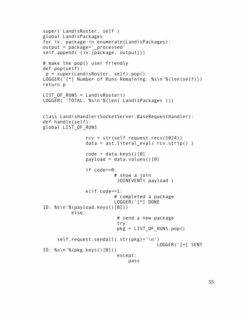
55

super( LandisRoster, self ) global LandisPackages for ix, package in enumerate(LandisPackages): output = package+'_processed' self.append( {ix:[package, output]}) # make the pop() user friendly def pop(self): p = super(LandisRoster, self).pop() LOGGER('[*] Number of Runs Remaining: %s\n'%(len(self))) return p LIST_OF_RUNS = LandisRoster() LOGGER( 'TOTAL: %s\n'%(len( LandisPackages ))) class LandisHandler(SocketServer.BaseRequestHandler): def handle(self): global LIST_OF_RUNS rcv = str(self.request.recv(1024)) data = ast.literal_eval( rcv.strip() ) code = data.keys()[0] payload = data.values()[0] if code==0: # show a join JOINEVENT( payload ) elif code==1: # completed a package LOGGER('[*] DONE ID: %s\n'%(payload.keys()[0])) else: # send a new package try: pkg = LIST_OF_RUNS.pop() self.request.sendall( str(pkg)+'\n') LOGGER('[+] SENT ID: %s\n'%(pkg.keys()[0])) except: pass

56

if __name__ == "__main__": CONNECT()

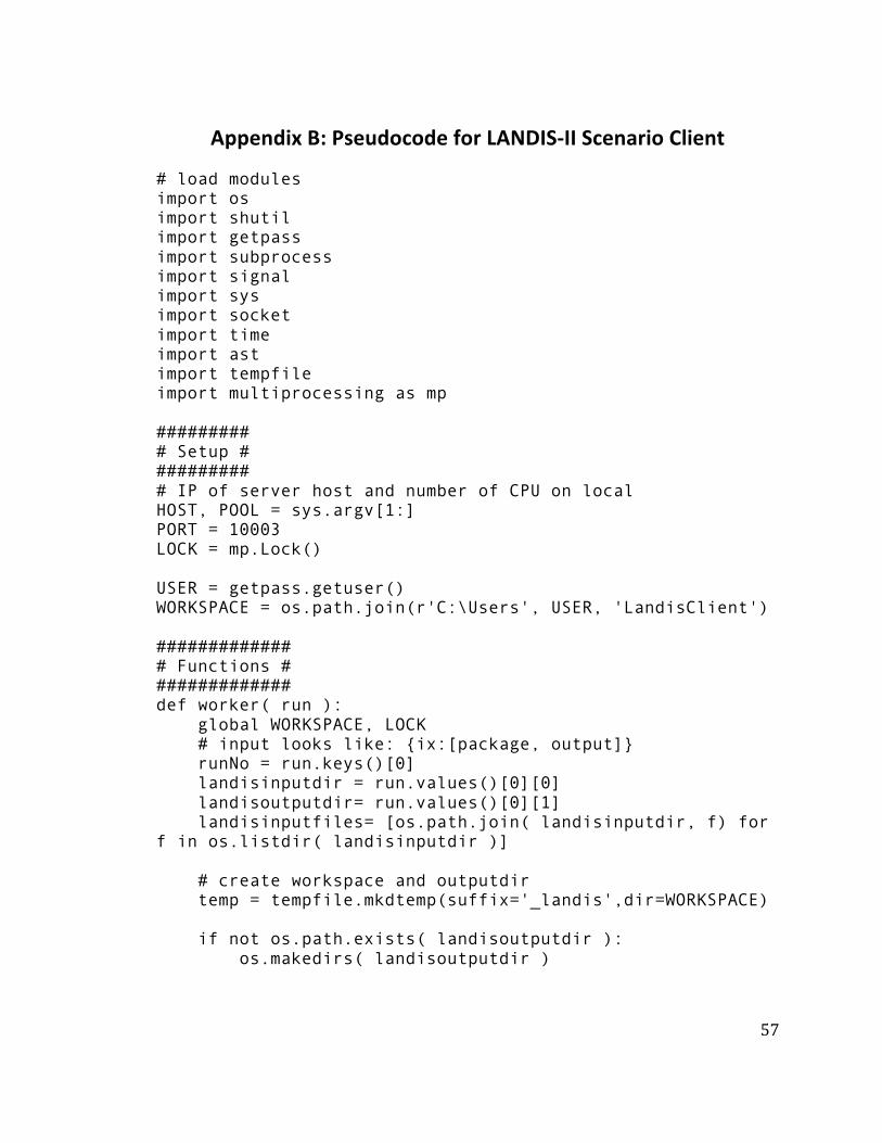
57

Appendix B: Pseudocode for LANDIS-‐II Scenario Client

# load modules import os import shutil import getpass import subprocess import signal import sys import socket import time import ast import tempfile import multiprocessing as mp ######### # Setup # ######### # IP of server host and number of CPU on local HOST, POOL = sys.argv[1:] PORT = 10003 LOCK = mp.Lock() USER = getpass.getuser() WORKSPACE = os.path.join(r'C:\Users', USER, 'LandisClient') ############# # Functions # ############# def worker( run ): global WORKSPACE, LOCK # input looks like: {ix:[package, output]} runNo = run.keys()[0] landisinputdir = run.values()[0][0] landisoutputdir= run.values()[0][1] landisinputfiles= [os.path.join( landisinputdir, f) for f in os.listdir( landisinputdir )] # create workspace and outputdir temp = tempfile.mkdtemp(suffix='_landis',dir=WORKSPACE) if not os.path.exists( landisoutputdir ): os.makedirs( landisoutputdir )

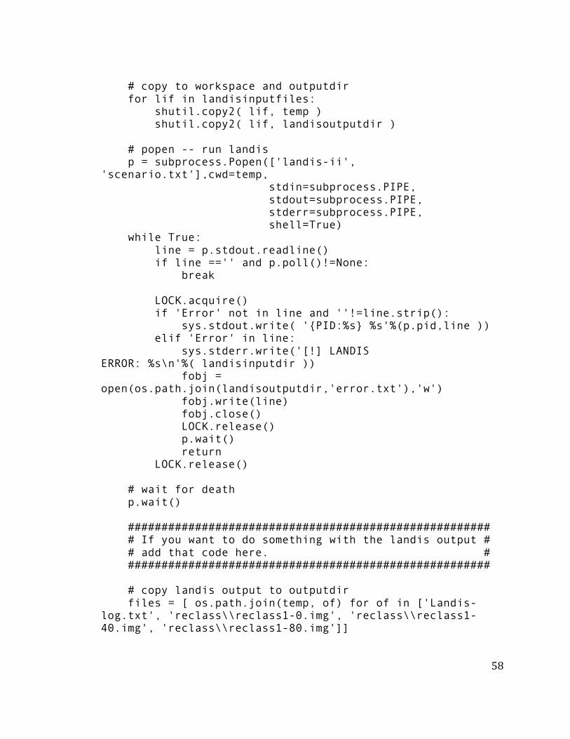
58

# copy to workspace and outputdir for lif in landisinputfiles: shutil.copy2( lif, temp ) shutil.copy2( lif, landisoutputdir ) # popen -- run landis p = subprocess.Popen(['landis-ii', 'scenario.txt'],cwd=temp, stdin=subprocess.PIPE, stdout=subprocess.PIPE, stderr=subprocess.PIPE, shell=True) while True: line = p.stdout.readline() if line =='' and p.poll()!=None: break LOCK.acquire() if 'Error' not in line and ''!=line.strip(): sys.stdout.write( '{PID:%s} %s'%(p.pid,line )) elif 'Error' in line: sys.stderr.write('[!] LANDIS ERROR: %s\n'%( landisinputdir )) fobj = open(os.path.join(landisoutputdir,'error.txt'),'w') fobj.write(line) fobj.close() LOCK.release() p.wait() return LOCK.release() # wait for death p.wait() ###################################################### # If you want to do something with the landis output # # add that code here. # ###################################################### # copy landis output to outputdir files = [ os.path.join(temp, of) for of in ['Landis-log.txt', 'reclass\\reclass1-0.img', 'reclass\\reclass1-40.img', 'reclass\\reclass1-80.img']]

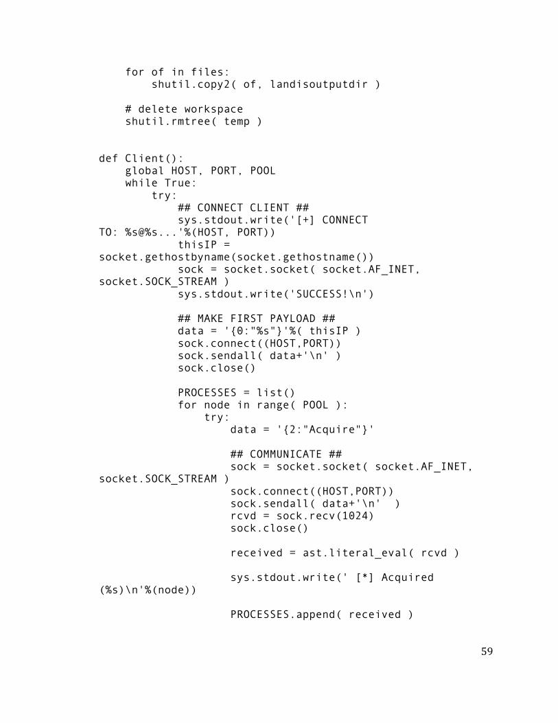
59

for of in files: shutil.copy2( of, landisoutputdir ) # delete workspace shutil.rmtree( temp ) def Client(): global HOST, PORT, POOL while True: try: ## CONNECT CLIENT ## sys.stdout.write('[+] CONNECT TO: %s@%s...'%(HOST, PORT)) thisIP = socket.gethostbyname(socket.gethostname()) sock = socket.socket( socket.AF_INET, socket.SOCK_STREAM ) sys.stdout.write('SUCCESS!\n') ## MAKE FIRST PAYLOAD ## data = '{0:"%s"}'%( thisIP ) sock.connect((HOST,PORT)) sock.sendall( data+'\n' ) sock.close() PROCESSES = list() for node in range( POOL ): try: data = '{2:"Acquire"}' ## COMMUNICATE ## sock = socket.socket( socket.AF_INET, socket.SOCK_STREAM ) sock.connect((HOST,PORT)) sock.sendall( data+'\n' ) rcvd = sock.recv(1024) sock.close() received = ast.literal_eval( rcvd ) sys.stdout.write(' [*] Acquired (%s)\n'%(node)) PROCESSES.append( received )

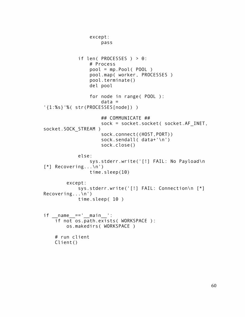
60

except: pass if len( PROCESSES ) > 0: # Process pool = mp.Pool( POOL ) pool.map( worker, PROCESSES ) pool.terminate() del pool for node in range( POOL ): data = '{1:%s}'%( str(PROCESSES[node]) ) ## COMMUNICATE ## sock = socket.socket( socket.AF_INET, socket.SOCK_STREAM ) sock.connect((HOST,PORT)) sock.sendall( data+'\n') sock.close() else: sys.stderr.write('[!] FAIL: No Payload\n [*] Recovering...\n') time.sleep(10) except: sys.stderr.write('[!] FAIL: Connection\n [*] Recovering...\n') time.sleep( 10 ) if __name__=='__main__': if not os.path.exists( WORKSPACE ): os.makedirs( WORKSPACE ) # run client Client()

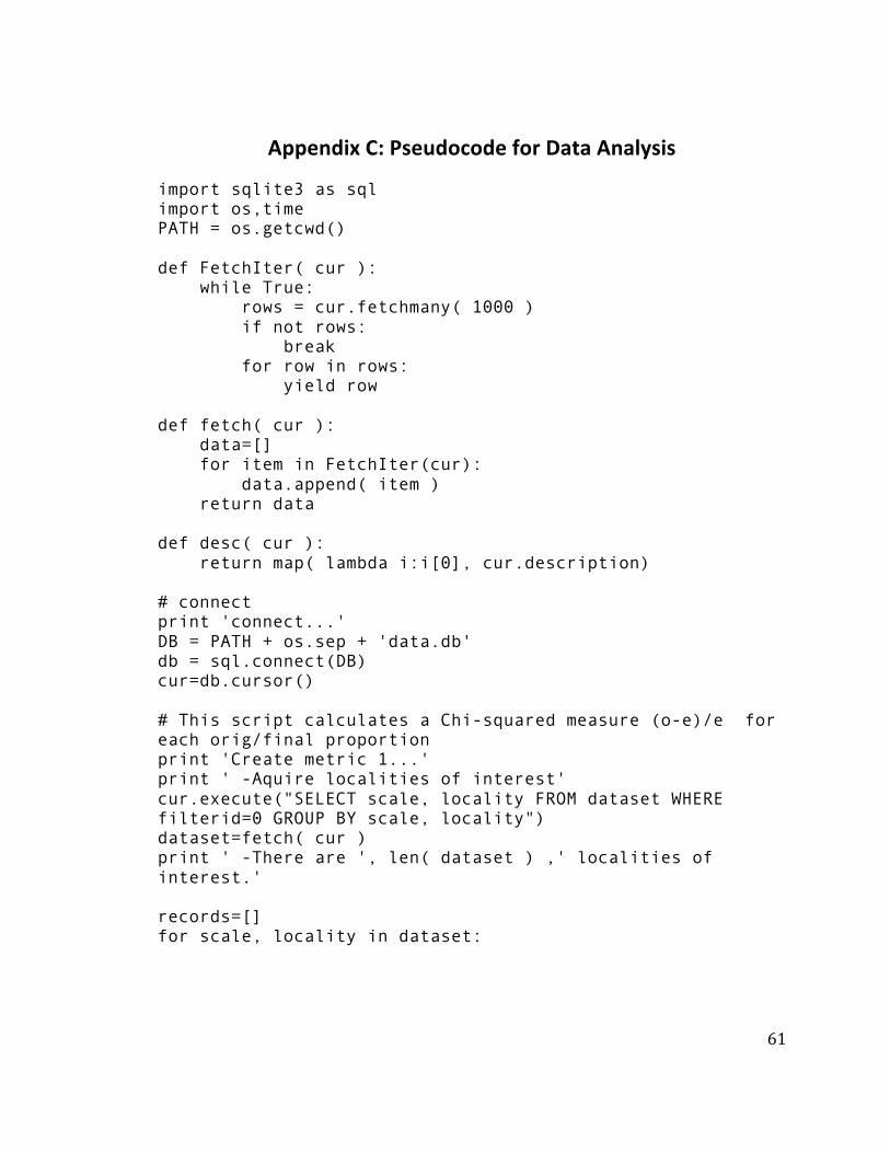
61

Appendix C: Pseudocode for Data Analysis

import sqlite3 as sql import os,time PATH = os.getcwd() def FetchIter( cur ): while True: rows = cur.fetchmany( 1000 ) if not rows: break for row in rows: yield row def fetch( cur ): data=[] for item in FetchIter(cur): data.append( item ) return data def desc( cur ): return map( lambda i:i[0], cur.description) # connect print 'connect...' DB = PATH + os.sep + 'data.db' db = sql.connect(DB) cur=db.cursor() # This script calculates a Chi-squared measure (o-e)/e for each orig/final proportion print 'Create metric 1...' print ' -Aquire localities of interest' cur.execute("SELECT scale, locality FROM dataset WHERE filterid=0 GROUP BY scale, locality") dataset=fetch( cur ) print ' -There are ', len( dataset ) ,' localities of interest.' records=[] for scale, locality in dataset:

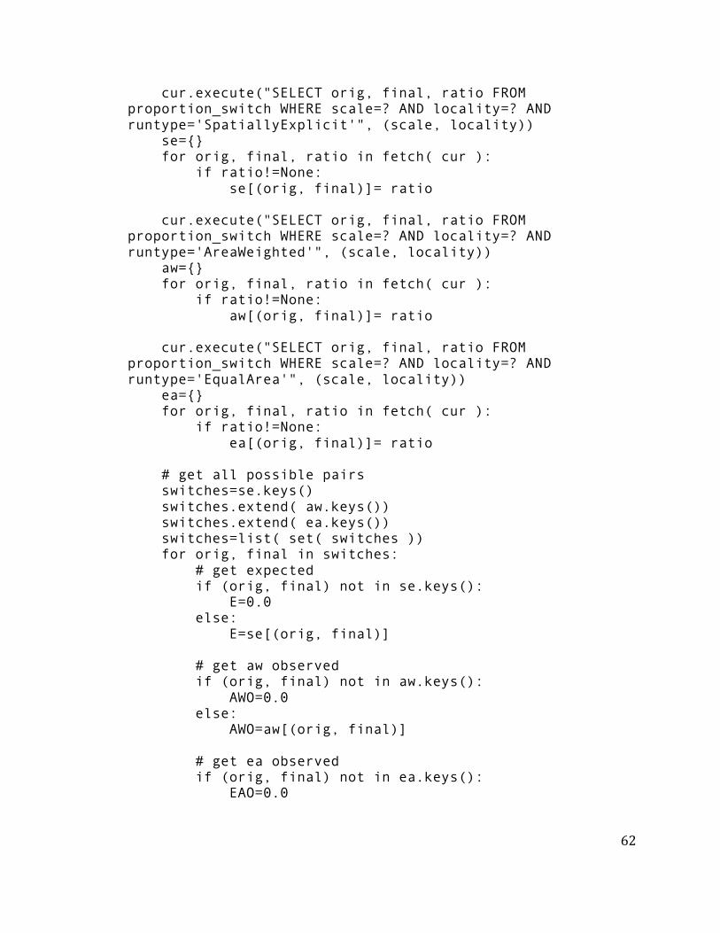
62

cur.execute("SELECT orig, final, ratio FROM proportion_switch WHERE scale=? AND locality=? AND runtype='SpatiallyExplicit'", (scale, locality)) se={} for orig, final, ratio in fetch( cur ): if ratio!=None: se[(orig, final)]= ratio cur.execute("SELECT orig, final, ratio FROM proportion_switch WHERE scale=? AND locality=? AND runtype='AreaWeighted'", (scale, locality)) aw={} for orig, final, ratio in fetch( cur ): if ratio!=None: aw[(orig, final)]= ratio cur.execute("SELECT orig, final, ratio FROM proportion_switch WHERE scale=? AND locality=? AND runtype='EqualArea'", (scale, locality)) ea={} for orig, final, ratio in fetch( cur ): if ratio!=None: ea[(orig, final)]= ratio # get all possible pairs switches=se.keys() switches.extend( aw.keys()) switches.extend( ea.keys()) switches=list( set( switches )) for orig, final in switches: # get expected if (orig, final) not in se.keys(): E=0.0 else: E=se[(orig, final)] # get aw observed if (orig, final) not in aw.keys(): AWO=0.0 else: AWO=aw[(orig, final)] # get ea observed if (orig, final) not in ea.keys(): EAO=0.0

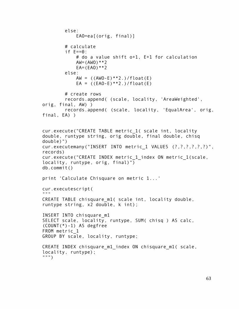
63

else: EAO=ea[(orig, final)] # calculate if E==0: # do a value shift o+1, E+1 for calculation AW=(AWO)**2 EA=(EAO)**2 else: AW = ((AWO-E)**2.)/float(E) EA = ((EAO-E)**2.)/float(E) # create rows records.append( (scale, locality, 'AreaWeighted', orig, final, AW) ) records.append( (scale, locality, 'EqualArea', orig, final, EA) ) cur.execute("CREATE TABLE metric_1( scale int, locality double, runtype string, orig double, final double, chisq double)") cur.executemany("INSERT INTO metric_1 VALUES (?,?,?,?,?,?)", records) cur.execute("CREATE INDEX metric_1_index ON metric_1(scale, locality, runtype, orig, final)") db.commit() print 'Calculate Chisquare on metric 1...' cur.executescript( """ CREATE TABLE chisquare_m1( scale int, locality double, runtype string, x2 double, k int); INSERT INTO chisquare_m1 SELECT scale, locality, runtype, SUM( chisq ) AS calc, (COUNT(*)-1) AS degfree FROM metric_1 GROUP BY scale, locality, runtype; CREATE INDEX chisquare_m1_index ON chisquare_m1( scale, locality, runtype); """)

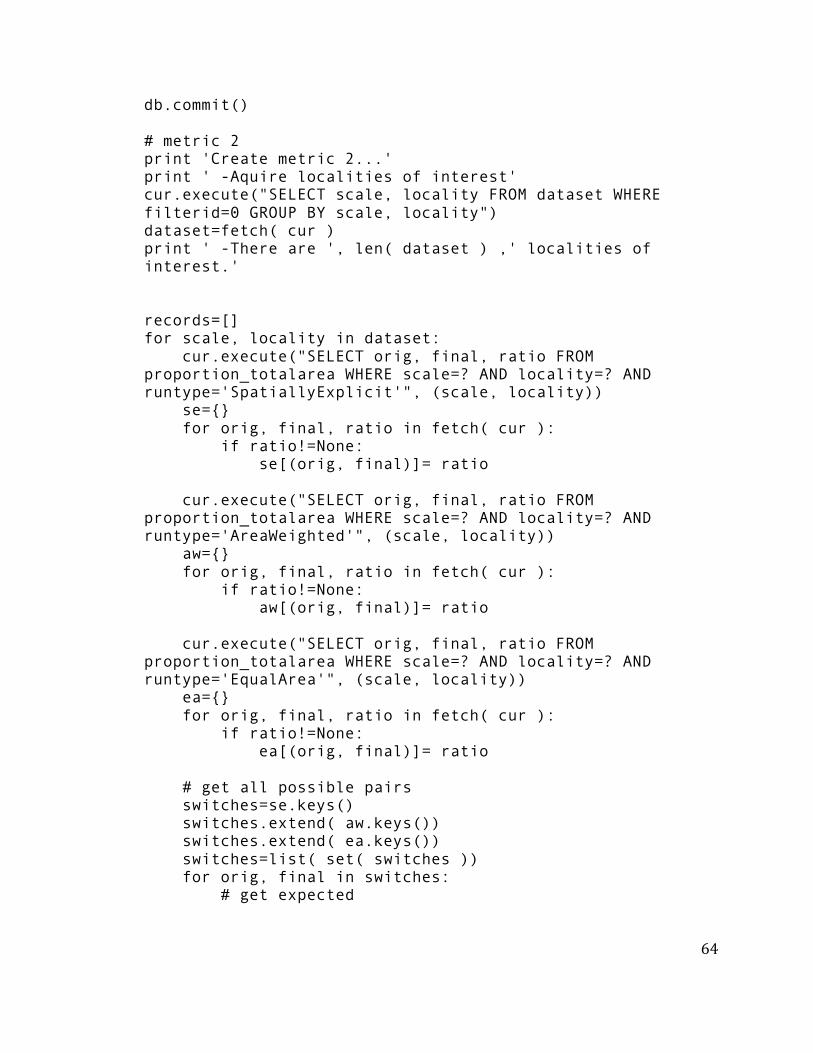
64

db.commit() # metric 2 print 'Create metric 2...' print ' -Aquire localities of interest' cur.execute("SELECT scale, locality FROM dataset WHERE filterid=0 GROUP BY scale, locality") dataset=fetch( cur ) print ' -There are ', len( dataset ) ,' localities of interest.' records=[] for scale, locality in dataset: cur.execute("SELECT orig, final, ratio FROM proportion_totalarea WHERE scale=? AND locality=? AND runtype='SpatiallyExplicit'", (scale, locality)) se={} for orig, final, ratio in fetch( cur ): if ratio!=None: se[(orig, final)]= ratio cur.execute("SELECT orig, final, ratio FROM proportion_totalarea WHERE scale=? AND locality=? AND runtype='AreaWeighted'", (scale, locality)) aw={} for orig, final, ratio in fetch( cur ): if ratio!=None: aw[(orig, final)]= ratio cur.execute("SELECT orig, final, ratio FROM proportion_totalarea WHERE scale=? AND locality=? AND runtype='EqualArea'", (scale, locality)) ea={} for orig, final, ratio in fetch( cur ): if ratio!=None: ea[(orig, final)]= ratio # get all possible pairs switches=se.keys() switches.extend( aw.keys()) switches.extend( ea.keys()) switches=list( set( switches )) for orig, final in switches: # get expected

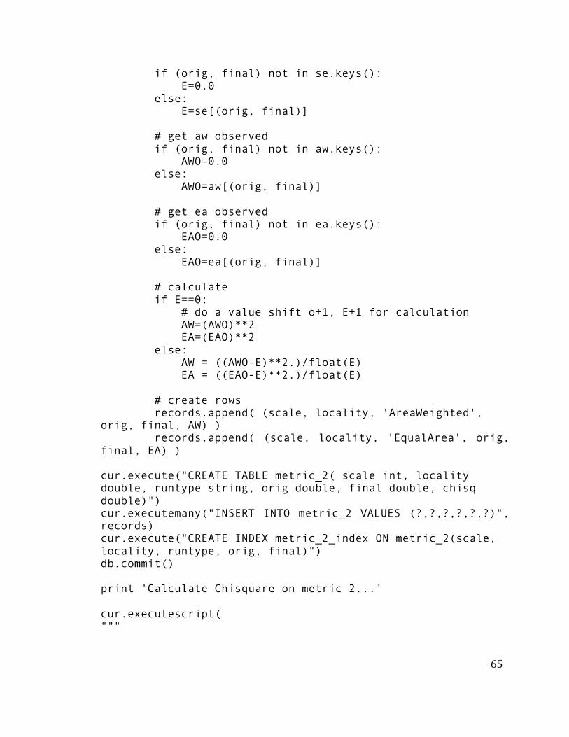
65

if (orig, final) not in se.keys(): E=0.0 else: E=se[(orig, final)] # get aw observed if (orig, final) not in aw.keys(): AWO=0.0 else: AWO=aw[(orig, final)] # get ea observed if (orig, final) not in ea.keys(): EAO=0.0 else: EAO=ea[(orig, final)] # calculate if E==0: # do a value shift o+1, E+1 for calculation AW=(AWO)**2 EA=(EAO)**2 else: AW = ((AWO-E)**2.)/float(E) EA = ((EAO-E)**2.)/float(E) # create rows records.append( (scale, locality, 'AreaWeighted', orig, final, AW) ) records.append( (scale, locality, 'EqualArea', orig, final, EA) ) cur.execute("CREATE TABLE metric_2( scale int, locality double, runtype string, orig double, final double, chisq double)") cur.executemany("INSERT INTO metric_2 VALUES (?,?,?,?,?,?)", records) cur.execute("CREATE INDEX metric_2_index ON metric_2(scale, locality, runtype, orig, final)") db.commit() print 'Calculate Chisquare on metric 2...' cur.executescript( """

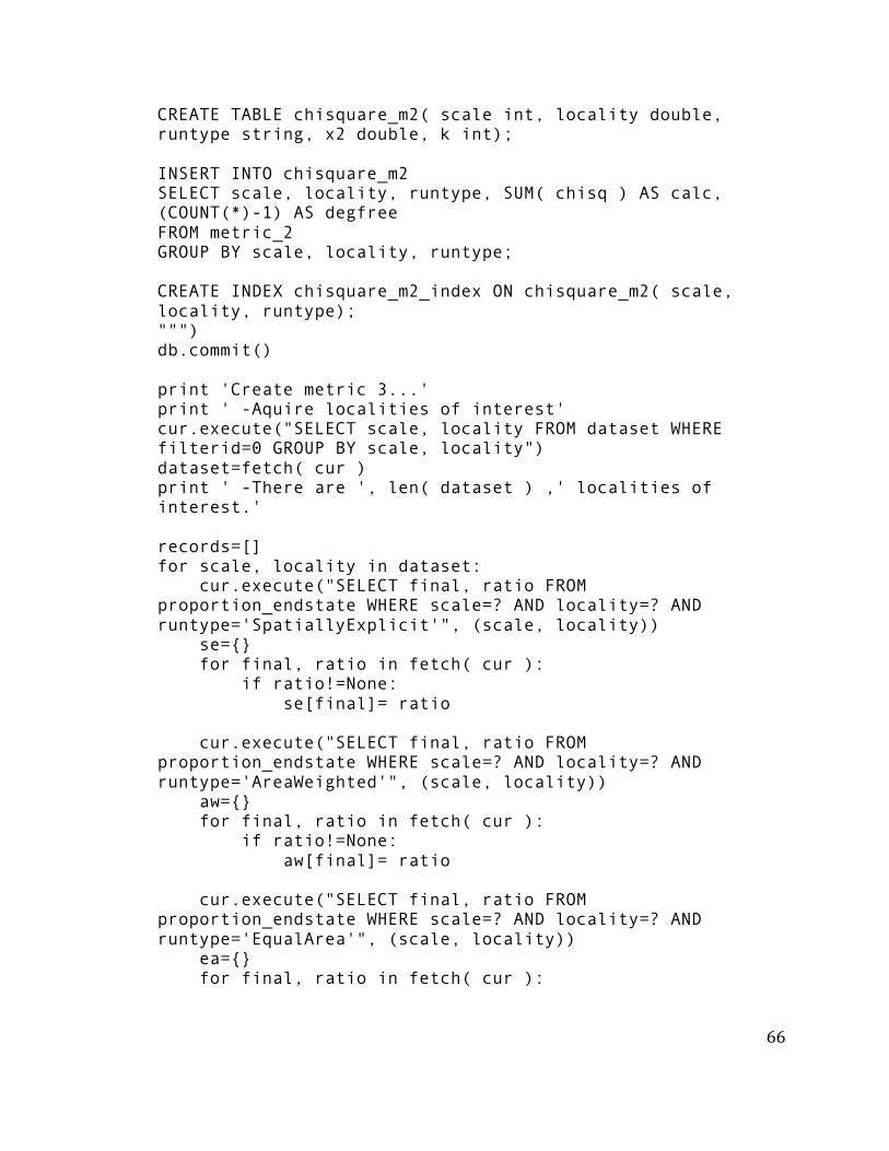
66

CREATE TABLE chisquare_m2( scale int, locality double, runtype string, x2 double, k int); INSERT INTO chisquare_m2 SELECT scale, locality, runtype, SUM( chisq ) AS calc, (COUNT(*)-1) AS degfree FROM metric_2 GROUP BY scale, locality, runtype; CREATE INDEX chisquare_m2_index ON chisquare_m2( scale, locality, runtype); """) db.commit() print 'Create metric 3...' print ' -Aquire localities of interest' cur.execute("SELECT scale, locality FROM dataset WHERE filterid=0 GROUP BY scale, locality") dataset=fetch( cur ) print ' -There are ', len( dataset ) ,' localities of interest.' records=[] for scale, locality in dataset: cur.execute("SELECT final, ratio FROM proportion_endstate WHERE scale=? AND locality=? AND runtype='SpatiallyExplicit'", (scale, locality)) se={} for final, ratio in fetch( cur ): if ratio!=None: se[final]= ratio cur.execute("SELECT final, ratio FROM proportion_endstate WHERE scale=? AND locality=? AND runtype='AreaWeighted'", (scale, locality)) aw={} for final, ratio in fetch( cur ): if ratio!=None: aw[final]= ratio cur.execute("SELECT final, ratio FROM proportion_endstate WHERE scale=? AND locality=? AND runtype='EqualArea'", (scale, locality)) ea={} for final, ratio in fetch( cur ):

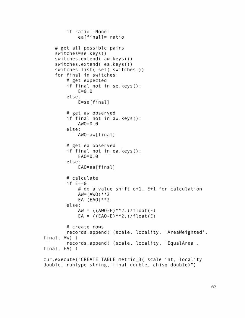
67

if ratio!=None: ea[final]= ratio # get all possible pairs switches=se.keys() switches.extend( aw.keys()) switches.extend( ea.keys()) switches=list( set( switches )) for final in switches: # get expected if final not in se.keys(): E=0.0 else: E=se[final] # get aw observed if final not in aw.keys(): AWO=0.0 else: AWO=aw[final] # get ea observed if final not in ea.keys(): EAO=0.0 else: EAO=ea[final] # calculate if E==0: # do a value shift o+1, E+1 for calculation AW=(AWO)**2 EA=(EAO)**2 else: AW = ((AWO-E)**2.)/float(E) EA = ((EAO-E)**2.)/float(E) # create rows records.append( (scale, locality, 'AreaWeighted', final, AW) ) records.append( (scale, locality, 'EqualArea', final, EA) ) cur.execute("CREATE TABLE metric_3( scale int, locality double, runtype string, final double, chisq double)")

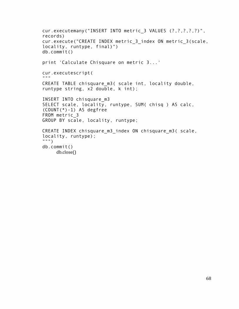
68

cur.executemany("INSERT INTO metric_3 VALUES (?,?,?,?,?)", records) cur.execute("CREATE INDEX metric_3_index ON metric_3(scale, locality, runtype, final)") db.commit() print 'Calculate Chisquare on metric 3...' cur.executescript( """ CREATE TABLE chisquare_m3( scale int, locality double, runtype string, x2 double, k int); INSERT INTO chisquare_m3 SELECT scale, locality, runtype, SUM( chisq ) AS calc, (COUNT(*)-1) AS degfree FROM metric_3 GROUP BY scale, locality, runtype; CREATE INDEX chisquare_m3_index ON chisquare_m3( scale, locality, runtype); """) db.commit()

db.close()

TESTING!LANDIS+IITOSTOCHASTICALLY! …

Documents

Transcript of TESTING!LANDIS+IITOSTOCHASTICALLY! …