arX

iv:g

r-qc

/041

1140

v1 2

9 N

ov 2

004

Testing the

Master Constraint Programme

for Loop Quantum Gravity

III. SL(2,R) Models

B. Dittrich∗, T. Thiemann†

Albert Einstein Institut, MPI f. GravitationsphysikAm Muhlenberg 1, 14476 Potsdam, Germany

and

Perimeter Institute for Theoretical Physics31 Caroline Street North, Waterloo, ON N2L 2Y5, Canada

Preprint AEI-2004-118

Abstract

This is the third paper in our series of five in which we test the Master ConstraintProgramme for solving the Hamiltonian constraint in Loop Quantum Gravity. In this workwe analyze models which, despite the fact that the phase space is finite dimensional, aremuch more complicated than in the second paper: These are systems with an SL(2,R) gaugesymmetry and the complications arise because non – compact semisimple Lie groups are notamenable (have no finite translation invariant measure). This leads to severe obstacles in therefined algebraic quantization programme (group averaging) and we see a trace of that in thefact that the spectrum of the Master Constraint does not contain the point zero. However,the minimum of the spectrum is of order ~2 which can be interpreted as a normal orderingconstant arising from first class constraints (while second class systems lead to ~ normalordering constants). The physical Hilbert space can then be be obtained after subtractingthis normal ordering correction.

∗dittrich@aei.mpg.de, bdittrich@perimeterinstitute.ca†thiemann@aei.mpg.de, tthiemann@perimeterinstitute.ca

1

Contents

1 Introduction 2

2 SL(2,R) Model with Non – Compact Gauge Orbits 42.1 Quantization . . . . . . . . . . . . . . . . . . . . . . . . . . . . . . . . . . . . . . 42.2 The Oscillator Representations and its Reduction . . . . . . . . . . . . . . . . . . 52.3 The Physical Hilbert space . . . . . . . . . . . . . . . . . . . . . . . . . . . . . . 7

3 Model with Two Hamiltonian Constraints and Non – Compact Gauge Orbits 83.1 Introduction of the Model . . . . . . . . . . . . . . . . . . . . . . . . . . . . . . . 83.2 Quantization . . . . . . . . . . . . . . . . . . . . . . . . . . . . . . . . . . . . . . 103.3 The Oscillator Representation . . . . . . . . . . . . . . . . . . . . . . . . . . . . . 103.4 The Spectrum of the Master Constraint Operator . . . . . . . . . . . . . . . . . . 123.5 The Physical Hilbert space . . . . . . . . . . . . . . . . . . . . . . . . . . . . . . 143.6 Algebraic Quantization . . . . . . . . . . . . . . . . . . . . . . . . . . . . . . . . . 15

4 Conclusions 17

A Review of the Representation Theory of SL(2,R) and its various Covering Groups 18A.1 sl(2,R) Representations . . . . . . . . . . . . . . . . . . . . . . . . . . . . . . . . 18A.2 Oscillator Representations . . . . . . . . . . . . . . . . . . . . . . . . . . . . . . 20

A.2.1 The Oscillator Representation . . . . . . . . . . . . . . . . . . . . . . . . . 20A.2.2 Contragredient Oscillator Representations . . . . . . . . . . . . . . . . . . 21A.2.3 Tensor Products of Oscillator Representations . . . . . . . . . . . . . . . . 21

A.3 Explicit Calculations for Example 3 . . . . . . . . . . . . . . . . . . . . . . . . . 24

1 Introduction

We continue our test of the Master Constraint Programme [1] for Loop Quantum Gravity (LQG)[6, 7, 8] which we started in the companion papers [2, 3] and will continue in [4, 5]. The MasterConstraint Programme is a new idea to improve on the current situation with the Hamiltonianconstraint operator for LQG [9]. In short, progress on the solution of the Hamiltonian constrainthas been slow because of a technical reason: the Hamiltonian constraints themselves are notspatially diffeomorphism invariant. This means that one cannot first solve the spatial diffeo-morphism constraints and then the Hamiltonian constraints because the latter do not preservethe space of solutions to the spatial diffeomorphism constraint [10]. On the other hand, thespace of solutions to the spatial diffeomorphism constraint [10] is relatively easy to constructstarting from the spatially diffeomorphism invariant representations on which LQG is based [11]which are therefore very natural to use and, moreover, essentially unique. Therefore one wouldreally like to keep these structures. The Master Constraint Programme removes that techni-cal obstacle by replacing the Hamiltonian constraints by a single Master Constraint which is aspatially diffeomorphism invariant integral of squares of the individual Hamiltonian constraintswhich encodes all the necessary information about the constraint surface and the associatedinvariants. See e.g. [1, 2] for a full discussion of these issues. Notice that the idea of squaringconstraints is not new, see e.g. [13], however, our concrete implementation is new and also theDirect Integral Decomposition (DID) method for solving them, see [1, 2] for all the details.

The Master Constraint for four dimensional General Relativity will appear in [14] but beforewe test its semiclassical limit, e.g. using the methods of [15, 16] and try to solve it by DIDmethods we want to test the programme in the series of papers [2, 3, 4, 5]. In the previouspapers we focussed on finite dimensional systems of various degrees of complexity. In this article

2

we will apply the Master Constraint Progamme to constraint algebras which generate a non-abelean and non-compact gauge group. In the first example we are concerned with the gaugegroup SO(2, 1) and in the second example with the gauge group SL(2,R), which is the doublecover of SO(2, 1).

We will see that both examples share the same problem – the spectrum of the MasterConstraint Operator does not include the value zero. The reason for this is the following: Thevalue zero in the spectrum of the Master Constraint Operator corresponds to the appearence ofthe trivial representation in a Hilbert space decomposition of the given unitary representationof the gauge group on the kinematical Hilbert space.

Now, the groups SO(2, 1) and SL(2,R) (and all groups which have these two groups assubgroups, e.g. symplectic groups and SO(p, q) with p, q > 1 and p+ q > 2 ) are non-amenablegroups, see [18]. One characteristic of non-amenable groups is, that the trivial representationdoes not appear in a Hilbert space decomposition of the regular representation into irreducibleunitary subrepresentations. Since the decomposition of the regular decomposition is often used todecompose tensor products, it will often happen, that a given representation of a non-amenablegroup does not include the trivial representation in its Hilbert space decomposition.

Since the value zero is not included in the spectrum of the Master Constraint Operator M we

will use a redefined operator M′= M−λmin as proposed in [2], where λmin is the minimum of the

spectrum. One can interprete this procedure as a quantum correction (which is proportional to~2). Nevertheless the redefinition of the Master Constraint Operator has to be treated carefully,since it is not guaranteed that all relations between the observables implied by the constraintsare realized on the resulting physical Hilbert space. This phenomenon will occur in the secondexample. However we will show that it is possible to alter the Master Constraint Operator againand to obtain a physical quantum theory which has the correct classical limit.

In both examples we will use the representation theory of SL(2,R) and its covering groupsto find the spectra and the direct integral decompositions with respect to the Master ConstraintOperator. As we will see, the diagonalization of the Master Constraint Operator is equivalentto the diagonalization of the Casimir Operator of the given gauge group representation, whichin turn is equivalent to the decomposition of the given gauge group representation into a directsum and/or direct integral of irreducible unitary representations.

Furthermore, we will see that our examples exhibit the structure of a dual pair, see [21].These are defined to be two subgroups in a larger group, where one subgroup is the maximalcommutant of the other and vice versa. In our examples one subgroup is the group generatedby the observables and the other is the group generated by the constraints. Now, given thisstructure of dual pairs, one can show that the decomposition of the representation of the gaugegroup is equivalent to the reduction of the representation of the observable algebra (on thekinematical Hilbert space). This is explained in further detail in appendix A.2. In our examplesthis fact will help us to determine the induced representation of the observable algebra on thephysical Hilbert space. Moreover we can determine in this way the induced inner product onthe physical Hilbert space, so that it will not be necessary to perform all the steps of the directHilbert space decomposition as explained in [2] to find the physical inner product.

We summarized the representation theory of the sl(2,R) algebra in appendix A.1. AppendixA.2 explains the theory of oscillator representations for sl(2,R), which is havily used in thetwo examples. It also contains a discussion how the representation theory of dual pairs can beapplied to our and similar examples.

3

2 SL(2, R) Model with Non – Compact Gauge Orbits

Here we consider the configuration space R3 with the three so(2, 1)-generators as constraints:

Li = ǫkijxjpk, {Li, Lj} = ǫkijLk (2.1)

where ǫkij = gkmǫmij , ǫijk is totally antisymmetric with ǫ123 = 1 and gik is the inverse of the

metric gik = diag(+,+,−). Indices are raised and lowered with gik resp. gik and we sum overrepeated indices.

The gauge group SO(n, 1) was previously discussed in [29], where group averaging was usedto construct the physical Hilbert space. We will compare the results of [29] and the resultsobtained here at the end of the section.

The observable algebra of the system above is generated by

d = xipi e+ = xixi e− = pipi . (2.2)

This set of observables exhibits the commutation relations of the generators of the sl(2,R)-algebra (which coincides with so(2, 1)):

{d, e±} = ∓2e± {e+, e−} = 4d . (2.3)

We have the identityd2 − e+e− = LiL

i (2.4)

between the Casimirs of the constraint and observable algebra.

2.1 Quantization

We start with the auxilary Hilbert space L2(R3) of square integrable functions of the coordinates.The momentum operators are pj = −i(~)∂j and the xj act as multiplication operators. Therearises no factor ordering ambiguity for the quantization of the constraints, but to ensure a closedobservable algebra, we have to choose:

d = 12(xipi + pix

i) = xipi − 32 i~

e+ = xixi e− = pipi (2.5)

The commutators between constraints and between observables are then obtained by replacingthe Poisson bracket with 1

i~

[·, ·

].

The identity (2.4) is altered to be:

d2 − 12(e+e− + e−e+) − 3

4~2 = LiLi . (2.6)

(From now on we will skip the hats and set ~ to 1.)For the implementation of the Master Constraint Programme we have to construct the

spectral resolution of the M

M := L21 + L2

2 + L23 = LiLi + 2L2

3 = d2 − 12(e+e− + e−e+) − 3

4 + 2L23 . (2.7)

To this end we will use the following strategy: The operators M and L3 commute, so we candiagonalize them simultaneously. The diagonalization of L3 is easy to achieve, its spectrumbeing purely discrete, namely spec(L3) = Z. Now we can diagonalize M on each eigenspace ofL3 seperately. On these eigenspaces the diagonalization of M is equivalent to the diagonalizationof the so(2, 1)-Casimir LiL

i and because of identity (2.6) equivalent to the diagonalization of thesl(2,R)-Casimir C = −1

4(d2− 12(e+e−+e−e+)). As we will show below the sl(2,R)-representation

given by (2.5) is a tensor product of three representations, which are known as oscillator andcontragredient oscillator representations. To obtain the spectral resolution of the Casimir C, wewill reduce this tensor product into its irreducible components.

4

2.2 The Oscillator Representations and its Reduction

For the reduction process it will be very convenient to work with the following basis of thesl(2,R)-algebra:

h = 14 (e+ + e−) = 1

2(a†1a1 + a†2a2 − a†3a3 + 12)

n+ = −12(i d − 1

2 (e+ − e−)) = 12(a†1a

†1 + a†2a

†2 − a3a3)

n− = 12 (i d+ 1

2(e+ − e−)) = 12(a1a1 + a2a2 − a†3a

†3)

C = 14 (d2 − 1

2(e+e− + e−e+)) = −h2 + 12 (n+n− + n−n+) , (2.8)

with commutation and adjointness relations[h, n±

]= ±n±

[n+, n−

]= −2h (n+)† = n− . (2.9)

Here we introduced the anihilation and creation operators

ai = 1√2(xi + ipi) and a†i = 1√

2(xi − ipi) . (2.10)

Now it is easy to see that this representation is a tensor product of the following three sl(2,R)-representations:

hi = 12(a†iai + 1

2) for i = 1, 2 and h3 = −12(a†3a3 + 1

2)

n+i = 1

2a†ia

†i n+

3 = −12a3a3

n−i = 12aiai n−3 = −1

2a†3a

†3 (2.11)

These representations are known as oscillator representation ω (for i = 1, 2) and contragredi-ent oscillator representation ω∗ (for i = 3), see [19] and A.2, where these representations areexplained.

The oscillator representation is the sum of two irreducible representations, which are therepresentations D(1/2) and D(3/2) from the positive discrete series of the double cover ofSl(2,R) (corresponding to even and odd number Fock states). Similarly ω∗ ≃ D∗(1/2)⊕D∗(3/2),where D∗(1/2) and D∗(3/2) are from the negative discrete series.

As mentioned before we will reduce this tensor product to its irreducible subrepresentations inorder to obtain the spectrum of the Casimir (and with it the spectrum of the Master ConstraintOperator). In appendix A.2 one can find the general strategy and some formulas to reducesuch tensor products. Furthermore appendix A.1 reviews the sl(2,R)-representations, whichwill appear below.

To begin the reduction of ω ⊗ ω ⊗ ω∗ we will reduce ω ⊗ ω. This we can achieve by uti-lizising the observable L3. It commutes with the sl(2,R)-algebra (2.8), therefore according toSchur’s Lemma its eigenspaces are left invariant by the sl(2,R)-algebra, i.e. its eigenspaces aresubrepresentations of sl(2,R).

To diagonalize L3 and reduce the tensor product ω ⊗ ω we will employ the “polarized”anihilation and creation operators

A± =1√2(a1 ∓ ia2) A†

± =1√2(a1 ± ia2). (2.12)

With the help of these, we can write

h = 12(A†

+A+ +A†−A− − a†3a3 + 1

2)

n+ = A†+A

†− − 1

2a3a3

n− = A+A− − 12a

†3a

†3 (2.13)

L3 = A†+A+ −A†

−A− . (2.14)

5

In the following we will denote by |k+, k−, k3 > Fock states with respect to A†+, A†

− and a†3.The operator L3 acts on them diagonally. Its eigenspaces V (±j) corresponding to the eigenvalue±j, j ∈ N are generated by {|j, 0, k3 >, k3 ∈ N} and {|0, j, k3 >, k3 ∈ N} respectively, i.e. V (j) is(the closure of) the linear span of the |j, 0, k3 >’s resp. |0, j, k3 >’s and all vectors are obtained byapplying repeatedly n+ to them. These eigenspaces are invariant subspaces of the representation(2.13). This representation restricted to V (j) is still a tensor product representation, namelythe representation D(|j| + 1) ⊗ ω∗. Its factors are given by

h12|V (j) = 12(A†

+A+ +A†−A− + 1)|V (j) and h3|V (j) = −1

2(a†3a3 + 12)|V (j)

n+12|V (j) = A†

+A†−|V (j) and n+

3 |V (j) = −12a3a3

n−12|V (j) = A+A−|V (j) and n−3 |V (j) = −12a

†3a

†3 . (2.15)

Since h12 has a smallest eigenvalue 12 (|j|+1) on the subspace V (j), this subspace carries aD(|j|+

1)-representation from the positive discrete series (of SL(2,R)) with lowest weight 12(|j| + 1)

(see A.1).So far we have achieved the reduction ω ⊗ ω ⊗ ω∗ ≃ (D(1) ⊕ ∑∞

j=0 2D(j + 1)) ⊗ ω∗. Toreduce the representation (2.13) completely, we have to consider tensor products of the formD(|j| + 1) ⊗D∗(1/2) and D(|j| + 1) ⊗D∗(3/2). We take this reduction from [19], see also A.2and A.1 for a description of the sl(2,R)-representations, appearing below:

For j even, we have

D(|j| + 1) ⊗D∗(1/2) ≃∫ 1

2+i∞

12

P (t, 1/4)dµ(t) ⊕∑

l

D(|j| + 1/2 − 2l)

with 0 ≤ 2l < |j| − 1/2, l ∈ N

(2.16)

and for j odd we get

D(|j| + 1) ⊗D∗(1/2) ≃∫ 1

2+i∞

12

P (t,−1/4)dµ(t) ⊕∑

l

D(|j| + 1/2 − 2l)

with 0 ≤ 2l < |j| − 1/2, l ∈ N .

(2.17)

In particular, we have for j = 0

D(1) ⊗D∗(1/2) ≃∫ 1

2+i∞

12

P (t, 1/4)dµ(t) . (2.18)

The remainig tensor products are

D(1) ⊗D∗(3/2) ≃∫ 1

2+i∞

12

P (t,−1/4)dµ(t)

D(|j| + 1) ⊗D∗(3/2) ≃ D(|j|) ⊗D∗(1/2) for j > 0 . (2.19)

P (t, ǫ), ǫ = 14 ,−1

4 is the principal series (of the metaplectic group, i.e. the double cover ofSL(2,R)) characterized by an h-spectrum spec(h) = {ǫ+ z, z ∈ Z} and a Casimir C(P (t, ǫ)) =t(1 − t)Id. The measure dµ(t) is the Plancherel measure on the unitary dual of the metaplecticgoup.

6

The representations D(l+1/2), l ∈ N−{0} are positive discrete series representations of themetaplectic group. The h-spectrum in these representations is given by {1

2 (l+ 1/2) + n, n ∈ N}and the Casimir by C(D(l + 1/2)) = −1

4(l + 1/2)2 + 12(l + 1/2).

The spectrum of the Casimir C is non-degenerate on each tensor product D(k) ⊗D∗(l), l =12 ,

32 , i.e. the Casimir discriminates the irreducible representations, which appear in this tensor

product and the irreducible representations have multiplicity one. The spectrum of h is non-degenerate in each irreducible representation of the metaplectic group . This implies that wecan find a (generalized) basis |j, ǫ, c, h >, which is labeled by the L3-eigenvalue j, the valuesǫ = 1

4 ,−14 , the Casimir eigenvalue c and the h-eigenvalue h.

Summarizing, we have for the (highly degenerate) spectrum of the Casimir C = −h2 +12(n+n− + n−n+) on L2(R3):

spec(C) = {14 + x2, x ∈ R, x ≥ 0} ∪ {−1

4 (l + 1/2)2 + 12(l + 1/2), l ∈ N − {0}} . (2.20)

The continuous part of the spectrum originates from the principal series P (t, 1/4) and P (t,−1/4)and the discrete part from those positive discrete series representations D(l), which appear inthe decompositions above. This results in the following expression for the spectrum of theso(2, 1)-Casimir LiLi = (4C − 3

4):

spec(LiLi) = {14 + s2, s ∈ R s ≥ 0} ∪ {−q2 + q, q ∈ N − {0}} . (2.21)

As explained in appendix A.1 these values correspond to the principal series P (12 + s, 0) of

SO(2, 1) and the positive or negative discrete series D(2q) resp. D∗(2q) for q ∈ N−{0}. In theSO(2, 1)-principal series the spectrum of L3 is given by spec(L3) = {Z}. In the discrete seriesD(2q) we have spec(L3) = {q + n, n ∈ N} and in D∗(q) spec(L3) = {−q − n, n ∈ N}.

2.3 The Physical Hilbert space

Now we can determine the spectrum of the Master Constraint Operator M = LiLi + 2L2

3 on thej-eigenspaces V (j) of L3. From the principal series we get the continous part of the spectrum

speccont(M |V (j)) = {14 + s2 + 2j2, s ∈ R, s ≥ 0} (2.22)

and from the discrete series the discrete part (for j ≥ 1, since there is no discrete part for j = 0)

specdiscr(M |V (j)) = {(−q2 + q) + 2j2, q ∈ N, q ≤ |j|} ≥ 2 . (2.23)

(The inequality q ≤ |j| follows from the fact, that in a representation D(2q) or D∗(2q) we have|j| ≥ q for the L3-eigenvalues j.)

One can see immedeatily, that zero is not included in the spectrum of the Master Constraint,

the lowest generalized eigenvalue being 14 . Therefore we alter the Master Constraint to M

′=

M−14(~2) where appropriate powers of ~ have been restored. The generalized null eigenspace

of M′

is given by the linear span of all states |j = 0, ǫ, c = 14 , h >. The spectral measure of

M′induces a scalar product on this space, which can then be completed to a Hilbert space. In

particular with this scalar product one can normalize the states |j = 0, ǫ, c = 14 , h >, obtaining

an ortho-normal basis ||ǫ, h >>.This Hilbert space has to carry a unitary representation of the metaplectic group. Actu-

ally, it carries a sum of two irreducible representations P (t = 1/2, 1/4) and P (t = 1/2,−1/4),corresponding to the labels ǫ = 1/4 and ǫ = −1/4 of the basis {||ǫ, h >>}. States in theserepresentations are distinguished by the transformation under the reflection R3 : x3 7→ −x3,which is a group element of O(2, 1). As an operator on L2(R3) it acts as:

R3 : ψ(x1, x2, x3) 7→ ψ(x1, x2,−x3) . (2.24)

7

R3 acts on states with ǫ = 14 as the identity operator (since these states are linear combinations

of even number Fock states with respect to a†3) and on states with ǫ = −14 by multiplying them

with (−1) (since these states are linear combinations of odd number Fock states). It seemsnatural, to exclude the states with nontrivial behaviour under this reflection. This leaves uswith the unitary irreducible representation P (t = 1/2, 1/4). As explained in A.1 the action ofthe observable algebra sl(2,R) on the states ||h >>:= ||1/4, h >> is determined (up to a phase,which can be fixed by adjusting the phases of the states ||h >>) by this representation to be:

h||h >> = h||h >> (h ∈ {14 + Z})

n+||h >> = (h + 12)||h + 1 >>

n−||h >> = (h − 12)||h − 1 >> . (2.25)

This gives for matrix elements of the observables d and e± (see 2.5)

<< h′|d|h >> = i(h + 12)δh′,h+1 − i(h − 1

2)δh′,h−1 (2.26)

<< h′|e±|h >> = 2h δh′,h ± (h + 12)δh′,h+1 ± (h − 1

2)δh′,h−1 . (2.27)

The operators e+ = xixi and e− = pipi are indefinite operators, i.e. their spectra includepositive and negative numbers.

To sum up, we obtained a physical Hilbert space, which carries an irreducible unitary repre-sentation of the observable algebra. In contrast to these results the group averaging procedurein [29] leads to (two) superselection sectors and therefore to a reducible representation of theobservables. These sectors are functions with compact support inside the light cone and func-tions with compact support outside the light cone. Hence the observable e+ = xixi is eitherstrictly positive or strictly negative definite on theses superselection sectors. From that point ofview our physical Hilbert space is preferred because physically e+ should be indefinite. However,as mentioned in [29] the appearence of superselection sectors may depend on the choice of thedomain Φ, on which the group averaging procedure has to be defined and thus other choices ofΦ may not suffer from this superselection problem. We see, at least in this example, that theDID method outlined in [2] with the prescription given there gives a more natural and uniqueresult. However, as the given system lacks a realistic interpretation anyway, this difference mayjust be an artefact of a pathological model.

3 Model with Two Hamiltonian Constraints and Non – Com-

pact Gauge Orbits

3.1 Introduction of the Model

Here we consider a reparametrization invariant model introduced by Montesinos, Rovelli andT.T. in [23]. It has an Sl(2,R) gauge symmetry and a global O(2, 2) symmetry and has attractedinterest because its constraint structure is in some sense similar to the constraint structure foundin general relativity. Further work on this model has appeared in [24, 25, 26, 27] and referencestherein.

We will shortly summarize the classical (canonical) theory (see [23] for an extended discus-sion). The configuration space is R4 parametrized by coordinates (u1, u2) and (v1, v2) and thecanonically conjugated momenta are (p1, p2) and (π1, π2). The system is a totally constrained(first class) system. The constraints form a realization of an sl(2,R)-algebra:

H1 = 12(~p2 − ~v2) H2 = 1

2(~π2 − ~u2) D = ~u · ~p− ~v · ~π (3.1)

{H1,H2} = D {H1,D} = −2H1 {H2,D} = 2H2 (3.2)

8

The canonical Hamiltonian governing the time evolution (which is pure gauge) is H = N H1 +M H2 + λD where N,M and λ are Lagrange multipliers. Since H1 and H2 are quadratic inthe momenta and their Poisson bracket gives a constraint which is linear in the momenta, onecould say that this model has an analogy with general relativity. There, one has Hamiltonianconstraints H(x) quadratic in the momenta and diffeomorphism constraints D(x) linear in themomenta which have the Poisson structure {H(x),H(y)} ∼ δ(x − y)D(x) and {H(x),D(y)} ∼δ(x− y)H(x).

However, one can make the following canonical transformation to new canonical coordinates(Ui, Vi, Pi,Πi), i = 1, 2 that transforms the constraint into phase space functions which are linearin the momenta:

ui = 1√2(Ui + Πi) vi = 1√

2(Vi + Pi)

pi = 1√2(−Vi + Pi) πi = 1√

2(−Ui + Πi) (3.3)

H1 = −P1V1 − P2V2 H2 = −U1Π1 − U2Π2 D = P1U1 + P2U2 − V1Π1 − V2Π2 . (3.4)

These coordinates have the advantage, that the constraints act on the configuration variables(U1, V1) and (U2, V2) in the defining two-dimensional representation of sl(2,R) (i.e. by matrixmultiplication).

For reasons that will become clear later, it is easier for us to stick to the old coordinates(ui, vi, pi, πi).

Now we will list the Dirac observables of this system. They reflect the global O(2, 2)-symmetry of this model and are given by (see [23])

O12 = u1p2 − p1u2 O23 = u2v1 − p2π1

O13 = u1v1 − p1π1 O24 = u2v2 − p2π2

O14 = u1v2 − p1π2 O34 = π1v2 − v1π2 (3.5)

They constitute the Lie algebra so(2, 2) which is isomorphic to so(2, 1)×so(2, 1). A basis adaptedto the so(2, 1) × so(2, 1)-structure is (see [26])

Q1 = 12(O23 +O14) P1 = 1

2(O23 −O14)

Q2 = 12(−O13 +O24) P2 = 1

2(−O13 −O24)

Q3 = 12(O12 −O34) P3 = 1

2(O12 +O34) (3.6)

The Poisson brackets between these observables are

{Qi, Qj} = ǫ kij Qk {Pi, Pj} = ǫ k

ij Pk {Qi, Pj} = 0 (3.7)

where ǫ kij = glkǫijk, with glk being the inverse of the metric glk = diag(+1,+1,−1). The Levi-

Civita symbol ǫijk is totally antisymmetric with ǫ123 = 1 and we sum over repeated indices.Lateron the (ladder) operators Q± := 1√

2(Q1 ± iQ2) and P± := 1√

2(P1 ± iP2) will be usefull.

One can find the following identities between observables and constraints (see [26]):

Q21 +Q2

2 −Q23 = P 2

1 + P 22 − P 2

3 = 14 (D2 + 4H1H2) (3.8)

4Q3P3 = (~u2 − ~v2)(H1 +H2) − (~u · ~p+ ~v · ~π)D + (~u2 + ~v2)(H1 −H2) (3.9)

They imply that on the constraint hypersurface we have Qi = 0 ∀i or Pi = 0 ∀i. certainsubmanifold of the phase space R8. Notice that the constraint hypersurface consists of thedisjoint union of the following five varieties: {Qj = Pj = 0, j = 1, 2, 3}, {±Q3 > 0, P3 =0}, {Q3 = 0, ±P3 > 0}.

9

3.2 Quantization

For the quantization we will follow [23] and choose the coordinate representation where the mo-mentum operators act as derivative operators and the configuration operators as multiplicationoperators on the Hilbert space L2(R4) of square integrable functions ψ(~u,~v):

~pψ(~u,~v) = −i~~∇uψ(~u,~v) ~πψ(~u,~v) = −i~~∇vψ(~u,~v)

uiψ(~u,~v) = uiψ(~u,~v) viψ(~u,~v) = viψ(~u,~v) . (3.10)

In the following we will skip the hats and set ~ = 1.For the constraint algebra to close we have to quantize the constraints in the following way:

H1 = −12(∆u + ~v2) H2 = −1

2(∆v + ~u2) D = −i(~u · ~∇u − ~v · ~∇v)[H1,H2

]= iD

[D,H1

]= 2iH1

[D,H2

]= −2iH2 . (3.11)

There arises no factor ordering ambiguity for the quantization of the observable algebra. Thealgebraic properties are preserved in the quantization process, i.e. Poisson brackets betweenobservables Oij are simply replaced by −i

[·, ·

].

We introduce a more convenient basis for the constraints:

H+ = H1 +H2 H− = H1 −H2 D = D . (3.12)

H− is just the sum and difference of Hamiltonians for one-dimensional harmonic oscillators. (Itis the generator of the compact subgroup SO(2) of Sl(2,R) and has discrete spectrum in Z).The commutation relations are now:

[H−,D

]= −2iH+

[H+,D

]= −2iH−

[H+,H−

]= −2iD . (3.13)

The operatorC = 1

4(D2 +H2+ −H2

−) (3.14)

commutes with all three constraints (3.12), since it is the (quadratic) Casimir operator forsl(2, r) (see Appendix A.1). According to Schur’s lemma, it acts as a constant on the irreduciblesubspaces of the sl(2,R) representation given by (3.12).

The quantum analogs of the classical identities (3.8) are

Q21 +Q2

2 −Q23 = P 2

1 + P 22 − P 2

3 = 14(D2 +H2

+ −H2−) = C (3.15)

4Q3P3 = (~u2 − ~v2)(H+) − (~u · ~p+ ~v · ~π)D + (~u2 + ~v2)(H−) . (3.16)

3.3 The Oscillator Representation

We are interested in the spectral decomposition of the Master Constraint Operator, which wedefine as

M = D2 +H2+ +H2

− = 4C + 2H2−. (3.17)

The Master Constraint Operator is the sum of (a multiple of) the Casimir operator and H−,which commutes with the Casimir. Therefore we can diagonalize these two operators simul-taneously, obtaining a diagonalization of M. We can achieve a diagonalization of the Casimirby looking for the irreducible subspaces of the sl(2,R)-representation given by (3.12), since theCasimir acts as a multiple of the identity operator on these subspaces. Hence we will attemptdo determine the representation given by (3.12).

10

By introducing creation and annihilation operators

ai =1√2(ui + ∂ui

) a†i =1√2(ui − ∂ui

) (3.18)

bi =1√2(vi + ∂vi

) b†i =1√2(vi − ∂vi

) (3.19)

we can rewrite the constraints as

H− =∑

i=1,2

(a†iai − b†i bi) (3.20)

H+ = −1

2

∑

i=1,2

(a2i + (a†i )

2 + b2i + (b†i )2) (3.21)

D =i

2

∑

i=1,2

(−a2i + (a†i )

2 + b2i − (b†i )2) . (3.22)

This sl(2,R) representation is a tensor product of the following four representations (withi ∈ {1, 2}):

(h−)ui= a†iai +

1

2(h−)vi

= −b†ibi −1

2

(h+)ui= −1

2((a†i )

2 + a2i ) (h+)vi

= −1

2((b†i )

2 + b2i )

dui=i

2((a†i )

2 − a2i ) dvi

=i

2(−(b†i )

2 + b2i ) (3.23)

The ui-representations are known as oscillator representations ω and the vi-representations ascontragredient oscilalator representations ω∗, see appendix A.2 for a discussion of these repre-sentations. As is also explained there these representation are reducible into two irreducible rep-resentations D(1/2) and D(3/2) for the oscillator representation ω and D∗(1/2) and D∗(3/2) forthe contragredient oscillator representation ω∗. The representation D(1/2) respectively D∗(1/2)acts on the space of even number Fock states, whereas D(3/2) respectively D∗(3/2) acts on thespace of uneven Fock states. The representations D(1/2) and D(3/2) are members of the positivediscrete series (of the two-fold covering group of Sl(2,R)), D∗(1/2) and D∗(3/2) are membersof the negative discrete series. (We have listed all sl(2,R)-representations in appendix A.1.)

Our aim is to reduce the tensor product ω⊗ω⊗ω∗⊗ω∗ into its irreducible components. Theisotypical component with respect to the trivial representation would correspond to the physicalHilbert space. To begin with we consider the tensor product ω ⊗ ω. The discussion for ω∗ ⊗ ω∗

is analogous.To this end we utilize the observable O12 (and O34 for the tensor product ω∗ ⊗ ω∗). Since

O12 commutes with the sl(2,R)-generators the eigenspaces of O12 are sl(2,R)-invariant. Theobservable O12 is diagonal in the “polarized” Fock basis, which is defined as the Fock basis withrespect to the new creation and annihilation operators

A± =1√2(a1 ∓ ia2) A†

± =1√2(a†1 ± ia†2). (3.24)

The “polarized” creation and annihilation operators for the v-coordiantes are

B± =1√2(b1 ∓ ib2) B†

± =1√2(b†1 ± ib†2). (3.25)

11

With help of these operators we can write the sl(2,R)-generators for the ω ⊗ ω representationand for the ω∗ ⊗ ω∗ representation as

h−A = A†+A+ +A†

−A− + 1 h−B = −B†+B+ −B†

−B− − 1

hA+ = −(A+A− +A†+A

†−) h+B = −(B+B− +B†

+B†−)

dA = i(A†+A

†− −A+A−) dB = i(B+B− −B†

+B†−) (3.26)

and the observables O12 and O34 as

O12 = u1p2 − p1u2 = A†+A+ −A†

−A−

O34 = π1v2 − v1π2 = −B†+B+ +B†

−B− . (3.27)

The (common) eigenspaces (corresponding to the eigenvalues j, j′ ∈ Z) for these observablesare spanned by {|k+, k−, k′+, k

′− >; k+ − k− = j and k′− − k′+ = j′; k+, k−, k′+, k

′− ∈ N}, where

|k+, k−, k′+, k′− > denotes a Fock state with respect to the annihilation operatorsA+, A−, B+, B−.

A closer inspection reveals that these eigenspaces are indeed invariant under the sl(2,R)-algebra.The action of the sl(2,R)-algebra on each of the above subspaces is a realization of the tensor

product representation D(|j| + 1) ⊗D∗(|j′| + 1) (see A.1). That can be verified by consideringthe h−A- and the h−B-spectrum on these subspaces. The h−A-spectrum is bounded from belowby (|j|+1), whereas the h−B-spectrum is bounded from above by −(|j′|+1). This characterizesD(|j| + 1)- and D∗(|j′| + 1)-representations respectively.

Up to now we have achieved

ω ⊗ ω ⊗ ω∗ ⊗ ω∗ =

[D(1) ⊕

∞∑

k=2

2D(k)

]⊗

[D∗(1) ⊕

∞∑

k=2

2D∗(k)

]. (3.28)

For a complete reduction of ω⊗ω⊗ω∗ ⊗ω∗ we have to reduce the tensor products D(|j|+ 1)⊗D∗(|j′| + 1).

3.4 The Spectrum of the Master Constraint Operator

In [22] the decomposition of all possible tensor products between unitary irreducible represen-tations of SL(2, R) was achieved.

( Actually [22] considers only representations of SL(2,R)/ ± Id, i.e. representations withuneven j and j′. However the results generalize to representations with even j or j′. See [28]for a reduction of all tensor products of SL(2,R), using different methods.)

The strategy in this article is to calculate the spectral decomposition of the Casimir operator.Since the Casimir commutes with H− one can consider the Casimir operator on each eigenspaceof H−.

Since the Master Constraint Operator is the sum M = 4C + 2H− we can easily adapt theresults of [22] for the spectral decomposition of the Master Constraint Operator. In the followingwe will shortly summarize the results for the spectrum of the Master Constraint Operator. Theexplicit eigenfunctions are constructed in appendix A.3.

To this end we define the subspaces V (k, j, j′), k ∈ Z, |j| ∈ N by

H−|V (k,j,j′) = k and O12|V (k,j,j′) = j and O34|V (k,j,j′) = j′ . (3.29)

V (k, j, j′) is the H−-eigenspace corresponding to the eigenvalue k of the tensor product repre-sentation D(|j| + 1)⊗D∗(|j′|+ 1). Since the H−-spectrum is even for (j − j′) even and unevenfor (j − j′) uneven these subspaces are vacuous for k+ j − j′ uneven. One result of [22] is, thatthe spectrum of the Casimir operator is non-degenerate on these subspaces, which means that

12

there exists a generalized eigenbasis in L2(R4) labeled by (k, j, j′) and the eigenvalue λC of theCasimir.

The spectrum of the Casimir C on the subspace V (k, j, j′) has a discrete part only if k > 0for |j| − |j′| ≥ 2 or k < 0 for |j| − |j′| ≤ 2. There is no discrete part if ||j| − |j′|| < 2. Thediscrete part is for (j − j′) and k even

λC = t(1 − t) with t = 1, 2, . . . , 12min(|k|, ||j| − |j′||)

= 0,−2,−6, . . . . (3.30)

For (j − j′) and k odd we have

λC = t(1 − t) with t = 32 ,

52 , . . . ,

12min(|k|, ||j| − |j′||)

= −34 ,−15

4 ,−354 . . . . (3.31)

The continuous part is in all cases the same and given by:

λC = 14 + x2 with x ∈

[0,∞

). (3.32)

The discrete part corresponds to unitary irreducible representations from the positive and neg-ative discrete series of SL(2,R), the continous part corresponds to the (two) principal series ofSL(2,R) (see appendix A.1).

For the spectrum of the Master Constraint Operator we have to multiply with 4 and add2k2:

λM

= 4t(1 − t) + 2k2 ≥ 2k2 − k2 + 2|k|with t = 1, 2, . . . , 1

2min(|k|, ||j| − |j′||) for even k

with t = 32 ,

52 . . . ,

12min(|k|, ||j| − |j′||) for odd k

and (3.33)

λM

= 1 + x2 + 2k2 > 0 (3.34)

As one can immediately see, the spectrum does not include zero. Since we have no discretespectrum for k = 0 the lowest generalized eigenvalue for the master constraint is 1 from thecontinuous part.

We will attempt to overcome this problem by introducing a quantum correction to the MasterConstraint Operator. Since 1 is the minimum of the spectrum we substract 1 (~2 if units arerestored) from the Master Constraint Operator.

For the modified Master Constraint Operator we get one solution appearing in the spectraldecomposition for each value of j and j′. We call this solution |λC = 1

4 , k = 0, j, j′ > and thelinear span of these soltutions SOL′.(The above results show, that these quantum numbers aresufficient to label uniquely vectors in the kinematical Hilbert space.)

At the classical level we have several relations between observables, which are valid on theconstraint hypersurface. For a physical meaningful quantization we have to check, whether theserelations are valid or modified by quantum corrections.

For our modified Master Constraint Operator this seems not to be the case: At the classicallevel we have Q3 = 0 or P3 = 0. But on SOL′, these observables evaluate to:

Q3 |λC = 14 , k = 0, j, j′ > = 1

2(j − j′) |λC = 14 , k = 0, j, j′ >

P3 |λC = 14 , k = 0, j, j′ > = 1

2(j + j′) |λC = 14 , k = 0, j, j′ > . (3.35)

Since j and j′ are arbitrary whole numbers, both Q3 and P3 can have arbitrary large eigenvalues(on the same eigenvector) in SOL′.

13

To solve this problem, we will modify the Master Constraint Operator again, by adding aconstraint, which implements the condition Q3 = 0 or P3 = 0. Together with the identities(3.15) this would ensure that Qi = 0∀i or Pi = 0∀i modulo quantum corrections.

One possibility for the modified constraint is M′′

= M−1+(Q3P3)2.(This operator is hermi-

tian, since Q3 and P3 commute.) Because of the last relation of (3.15) this modification can beseen as adding the square (of one quarter) of the right hand side of this relation, i.e. the addedpart is the square of a linear combination of the constraints.

We already know the spectral resolution of M′′, since we used Q3 and P3 (or O12 and O34) in

the reduction process for the Master Constraint Operator. Solutions to the Master Constraint

Operator M′′

are the states |λC = 14 , k = 0, j, j′ > with |j| = |j′|. We call this solution space

SOL′′. (Up to now this spase is just the linear span of states |λC = 14 , k = 0, j, j′ > with

|j| = |j′|. Later we will specify a topology for this space.)Now the observable algebra (3.6) does not leave this solution space invariant, since not

all observables commute with the added constraint Q3P3. However, the observables (3.6) areredundant on SOL′′, since they obey the relations (3.15). So the question is, whether onecan find enough observables, which commute with Q3P3 (and with the constraints, we startedwith) to carry all relevant physical information. Apart from Q3 and P3 the operators Q2

1 +Q22

and P 21 + P 2

2 commute with the added constraint. But the latter do not carry additionalinformation about physical states, because of the first relation in (3.15). Operators of the formp1(Q)Q3 + p2(P )P3, where p1(Q) (resp. p2(P )) represents a polynomial in the Q-observables(P -observables), commute with Q3P3 on the subspace defined by Q3P3 = 0. Likewise operatorsof the form p1(Q)|sgn(Q3)| + p2(P )|sgn(P3)|, where sgn has values 1, 0 and −1 (and is definedby the spectral theorem) leave SOL′′ (formally) invariant.

In the following we will take as observable algebra the algebra generated by the elementaryoperators |sgn(Q3)|Qi|sgn(Q3)| and |sgn(P3)|Pi|sgn(P3)|. This algebra is closed under taking ad-joints. Notice, however, that we may add operators such as |sgn(Q3)|Q+Q+|sgn(Q3)| which doesnot leave the sectors invariant and thus destroy the superselection structure which is a physicaldifference from the results of [24]. The next section shows that the latter operator transformsstates from the sector {sgn(Q3) = −1, sgn(P3) = 0} to the sector {sgn(Q3) = +1, sgn(P3) = 0}(since Q±, P± are ladder operators, which raise or lower the Q3, P3 eigenvalues by 1 respec-tively). Likewise one can construct operators wich transform from the sector {sgn(P3) = 0} to{sgn(Q3) = 0} and vice versa: For instance

|sgn(P3)|P+ · · ·P+ (1 − |sgn(Q3)|)(1 − |sgn(P3)|)Q+ · · ·Q+ |sgn(Q3)| (3.36)

has this property and leaves the solution space to the modified Master Constraint Operatorinvariant. Its adjoint is of the same form, transforming from the sector {sgn(Q3) = 0} to thesector {sgn(P3) = 0}. Thus we may map between all five sectors mentioned before except forthe origin. There seems to be no natural exclusion principle for these operators from the pointof view of DID and thus we should take them seriously.

3.5 The Physical Hilbert space

Now one can use the spectral measure for the Master Constraint Operator and construct a scalarproduct in SOL′ and SOL′′ and then complete them into Hilbert spaces H′ and H′′. This isdone explicitly in Appendix A.3, here we only need that this can be done in principle.

The so achieved Hilbert space H′ has to carry a unitary representation of the observablealgebra sl(2,R)× sl(2,R) (since these observables commute with the constraints). In particularwe already know the spectra of Q3 and P3 to be the integers Z, since we diagonalized themsimultaneously with the Master Constraint Operator. These spectra are discrete, which meansthat in the constructed scalar product the states |λC = 1

4 , k = 0, j, j′ > (which are eigenstates

14

for Q3 and P3) have a finite norm. So we can normalize them to states ||j, j′ >> and in thisway obtain a basis of H′.

Now, because of the identity (3.15) we also know the value of the sl(2,R) Casimirs Q21+Q2

2−Q2

3 and P 21 +P 2

2 −P 23 on H′ to be 1

4 . Together with the fact that H′ has a normalized eigenbasis{||j, j′ >>, j, j′ ∈ Z} (with respect to Q3 and P3) we can determine the unitary representationof sl(2,R) × sl(2,R) to be P (t = 1/2, ǫ = 0)Q ⊗ P (t = 1/2, ǫ = 0)P (see Appendix A.1). Thisfixes the action of the (primary) observable algebra to be (modulo phase factors, which can bemade to unity by adjusting phases of the basis vectors):

Q+||j, j′ >> = 12√

2((j − j′) + 1) ||j + 1, j′ − 1 >>

Q−||j, j′ >> = 12√

2((j − j′) − 1) ||j − 1, j′ + 1 >>

Q3||j, j′ >> = 12(j − j′) ||j, j′ >>

P+||j, j′ >> =1

2√

2((j + j′) + 1) ||j + 1, j′ + 1 >>

P−||j, j′ >> =1

2√

2((j + j′) − 1) ||j − 1, j′ − 1 >>

P3||j, j′ >> = 12(j + j′)| |j, j′ >> (3.37)

From these results we can derive the action of the altered observable algebra on H′′, i.e. onstates ||j, ǫj >> with ǫ = ±1:

Θ(Q3)Q+Θ(Q3) ||j, ǫj >> = δ−1,ǫ (1 − δ−1,j)1√2(j + 1

2) ||j + 1, ǫ(j + 1) >>

Θ(Q3)Q−Θ(Q3) ||j, j′ >> = δ−1,ǫ (1 − δ+1,j)1√2(j − 1

2) ||j − 1, ǫ(j − 1) >>

Q3 ||j, ǫj >> = δ−1,ǫ j ||j, ǫj >>Θ(P3)P+Θ(P3) ||j, j′ >> = δ1,ǫ (1 − δ−1,j)

1√2

(j + 12) ||j + 1, ǫ(j + 1) >>

Θ(P3)P−Θ(P3) ||j, j′ >> = δ1,ǫ (1 − δ+1,j)1√2(j − 1

2) ||j − 1, ǫ(j − 1) >>

P3 ||j, ǫj >> = δ1,ǫ j ||j, ǫj >> (3.38)

where we abbreviated |sgn(O)| by Θ(O). The state |0, 0 > is annihilated by all (altered) ob-servables.

3.6 Algebraic Quantization

In [24] the SL(2,R)-model has been quantized in the Algebraic and Refined Algebraic Quanti-zation framework. We will shortly review the results of the Algebraic Quantization scheme inorder to compare them with the Master Constaint Programme.

In this scheme one starts with the auxilary Hilbert space L2(R4), the constraints (3.11)and a ∗- algebra of observables A∗. One looks for a solution space for the constraints whichcarries an irreducible representation of A∗ and for a scalar product on this space in which thestar-operation becomes the adjoint operation.

The solution space V , which was found in [24] is the linear span of states |j, ǫj > where j is inZ and ǫ ∈ {−1,+1}. These states are expressible as smooth functions on the (~u,~v) configurationspace R4 and they solve the constraints (3.11).

The solution states can be expressed in our “polarized” Fock basis as follows

|j, ǫj >=∑

m=0

(−1)m|m+ 12 (j + |j|),m + 1

2(−j + |j|) > ⊗

|m+ 12(−ǫj + |j|),m + 1

2 (ǫj + |j|) > . (3.39)

15

(These states are the solutions f(t = 1; k = 0, j, j′ = ǫj), see (A.3).) Clearly, the states |j, ǫj >solve the Master Constraint Operator M. However there are much more solutions to the MasterConstraint Operator (which do not necessarily solve the three constraints (3.11)).

The algebra A∗ used in [24] is the algebra generated by the observables (3.6). The star-operation is defined by Q∗

i = Qi, P∗i = Pi and extended to the full algebra by complex anti-

linearity. This algebra is supplemented to the algebra A∗ext by the operators Rǫ1,ǫ2 = R∗

ǫ1,ǫ2,which permute between the four different sectors of the classical constraint phase space:

Rǫ1,ǫ2 : (u1, u2, v1, v2, p1, p2, π1, π2) 7→ (u1, ǫ1u2, v1, ǫ1ǫ2v2, p1, ǫ1p2, π1, ǫ1ǫ2π2) (3.40)

The algebra A∗ has the following representation on V :

Q3|j, ǫj > = δ−1,ǫ j |j, ǫj >Q±|j, ǫj > = δ−1,ǫ ( ∓i√

2|j|) |(j ± 1), ǫ (j ± 1) >

P3|j, ǫj > = δ+1,ǫ j |j, ǫj >P±|j, ǫj > = δ+1,ǫ ( ∓i√

2|j|) |(j ± 1), ǫ (j ± 1) > (3.41)

The state |j = 0, j′ = 0 > is annihilated by all operators in A∗, in particular, it generates aninvariant subspace for A∗. Now, it is not possible to introduce an inner product on V , in whichthe star-operation becomes the adjoint operation (because the SO(2, 2)-representation definedby (3.41) is non-unitary). However, since |0, 0 > generates an invariant subspace one can takethe quotient V /{c|0, 0 >, c ∈ C}, consisting of equivalence classes

[v]

= {v + c |0, 0 >, c ∈ C}where v ∈ V . (In particular

[|0, 0 >

]is the null vector

[0].) The so(2, 2)-representation

on V then defines a representation on this quotient space by O([v]) = [O(v)], where O is anso(2, 2)-operator. (This representation is well defined because we are quotienting out an invariantsubspace.) A basis in this quotient space is {

[|j, ǫj >

], j ∈ N − {0}}. In the following we will

drop the equivalence class brackets [·].The quotient representation is the direct sum of four (unitary) irreducible representations of

so(2, 2), labeled by sgn(j) = ±1 and ǫ = ±1. The inner product, which makes these representa-tions unitary is

< j1, ǫ1j1|j2, ǫ2j2 >= c(sgn(j), ǫ) δj1 ,j2 δǫ1,ǫ2 |j| (3.42)

where c(sgn(j), ǫ) are four independent positiv constants.By taking the reflections Rǫ1,ǫ2 ∈ O(2, 2) into account, we can partially fix these constants.

Their action on states in L2(R4) is

(Rǫ1,ǫ2ψ)(u1, u2, v1, v2) = ψ(u1, ǫ1u2, v1, ǫ1ǫ2v2) . (3.43)

States with angular momenta j and j′ are mapped to states with angular momenta ǫ1j andǫ1ǫ2j

′. Therefore the Rǫ1,ǫ2’s effect, that the quotient representation of the observable algebrabecomes an irreducible one. Since Rǫ1,ǫ2 is in O(2, 2), it is a natural requirement for them to actby unitary operators. This fixes the four constants c(sgn(j), ǫ) to be equal (and in the followingwe will set them to 1).

This gives for the action of the algebra A∗ on the normalized basis vectors |j, ǫj >N :=1√|j||j, ǫ j >, j ∈ Z − {0}:

Q3|j, ǫj >N = δ−1,ǫ j |j, ǫj >N

Q±|j, ǫj >N = δ−1,ǫ ( ∓i√2

√|j(j ± 1)|) |(j ± 1), ǫ (j ± 1) >N

P3|j, ǫj >N = δ+1,ǫ j |j, ǫj >N

P±|j, ǫj >N = δ+1,ǫ ( ∓i√2

√|j(j ± 1)|) |(j ± 1), ǫ (j ± 1) >N . (3.44)

16

In the limit of large j the right hand sides of (3.38) and (3.44), ie. the matrix elements ofthe observables in the two qunatizations, coincide except for phase factors. These can be madeequal by adjusting the phase factors of the respective basic vectors. Therefore both quantizationprograms lead to the same semiclassical limit.

A first crucial difference in the results of the two quantization approaches is that in theMaster Constraint Programme the vector ||j = 0, j′ = 0 >> is included in the physical Hilbertspace whereas it is excluded during the Algebraic Quantization process. If we exclude the sectorchanging operators mentioned above by hand, then ||j = 0, j′ = 0 >> is annihilated by thealtered observable algebra and likewise cannot be reached by applying observables to other statesin the physical Hilbert space. If we include the sector changing operators then |j = 0, j′ = 0 > isstill not in the range of any observable because the observables are sandwiched beween operatorsof the form |sgn(Q3)|, |sgn(Q3)|. However, one can map between all the remaining sectors whichthus provides a second difference with [24].

4 Conclusions

What we learnt in this paper is that the Master Constraint Programme can also successfullybe applied to the difficult of constraint algebras generating non – amenable, non – compactgauge groups. As was observed for instance in [29] this is a complication which affects the groupaveraging proposal [12] for solving the quantum constraints quite drastically in the sense thatthe physical Hilbert space depends critically on the choice of a dense subspace of the Hilbertspace. The Master Constraint Programme also faces complications: The spectrum is supportedon a genuine subset of the positive real line not containing zero. Our proposal to subract thezero point of the spectrum from the Master Constraint, which can be considered as a quantumcorrection1 because it is proportional to ~2 worked and produced an acceptable physical Hilbertspace.

Of course, it is unclear whether that physical Hilbert space is in a sense the only correctchoice because the models discussed are themselves not very physical and therefore we haveonly mathematical consistency as a selection criterion at our disposal, such as the fact that thealgebraic approach reaches the same semiclassical limit by an independent method. Neverthe-less, it is important to notice that DID produces somewhat different results than algebraic andRAQ methods, in particular, the superselection theory is typically trivial in contrast to thoseprogrammes. It would be good to know the deeper or intuitive reason behind this and otherdifferences. Obviously, further work on non – amenable groups is necessary, preferrably in anexample which has a physical interpretation, in order to settle these interesting questions.

Acknowledgements

We thank Hans Kastrup for fruitful discussions about SL(2,R), especially for pointing outreference [22]. BD thanks the German National Merit Foundation for financial support. Thisresearch project was supported in part by a grant from NSERC of Canada to the PerimeterInstitute for Theoretical Physics.

1The fact that the correction is quadratic in ~ rather than linear in contrast to the normal ordering correctionof the harmonic osciallor can be traced back to the fact that harmonic oscillator Hamiltonian can be consideredthe Master Constraint for the second class pair of constraints p = q = 0 while the sl(2R) constraints are firstclass.

17

A Review of the Representation Theory of SL(2, R) and its var-

ious Covering Groups

A.1 sl(2, R) Representations

In this section we will review unitary representations of sl(2,R), see [31, 30].In the defining two-dimensional representation the sl(2,R)-algebra is spanned by

h =−1

2i

(0 1−1 0

)n1 =

−1

2i

(0 11 0

)n2 =

−1

2i

(1 00 −1

)(A.1)

with commutation relations

[h, n1

]= in2

[n2, h

]= in1

[n1, n2

]= −ih . (A.2)

We introduce raising and lowering operators n± as complex linear combinations n± = n1 ± in2

of n1 and n2, which fulfill the algebra

[h, n±

]= ±n±

[n+, n−

]= −2h . (A.3)

The Casimir operator, which commutes with all sl(2,R)-algebra operators, is

C = −h2 + 12(n+n− + n−n+) = −h2 + n2

1 + n22 . (A.4)

We are interested in unitary irreducible representations of sl(2,R), i.e. representations whereh, n1 and n2 act by self-adjoint operators on a Hilbert space, which does not have non-trivialsubspaces, that are left invariant by the sl(2,R)-operators. According to Schur’s Lemma theCasimir operator acts on an irreducible space as a multiple of the identity operator C = c Id.Since n1 and n2 are self-adjoint operators, the raising operator n+ is the adjoint of the loweringoperator n− and vice versa. (For notational convenience we often do not discriminate betweenelements of the algebra and the operators representing them.)

In general the sl(2,R)-representations do not exponentiate to a representation of the groupSL(2,R) but to the universal covering group ˜SL(2,R). Since h is the generator of the compactsubgroup of ˜SL(2,R) it will have discrete spectrum (and therefore normalizable eigenvectors)in a unitary representation. If the sl(2,R)-representation exponentiates to an SL(2,R) repre-sentation, h has spectrum in {1

2n, n ∈ Z}. If in this group representation the center ±Id actstrivially, it is also an SO(2, 1) representation, since SO(2, 1) is isomorphic to the quotient groupSL(2,R)/{±Id}. In this case h has spectrum in Z.

Now, assume that |h > is an eigenvector of h with eigenvalue h. Using the commutationrelations (A.3) one can see, that n±|h > is either zero or an eigenvector of h with eigenvalueh ± 1. By repeated application of n+ or n− to |h > one therefore obtains a set of eigenvectors{|h+n >} and corresponding eigenvalues {h+n}, where n is an integer. This set of eigenvaluesmay or may not be bounded from above or below.

Similarly, one can deduce from the commutation relations that n+n−|h > and n−n+|h > areboth eigenvectors of h with eigenvalue h (or zero). Apriori these eigenvectors do not have to bea multiple of |h >, since it may be, that h has degenerate spectrum. But this is excluded by therelations

n+n− = h2 − h+ C n−n+ = h2 + h+ C , (A.5)

obtained by using (A.3,A.4). (Remember, that h and C act as multiples of the identity on|h >.) From this one can conclude that the set {|h+n >} is invariant under the sl(2,R)-algebra(modulo multiples) and hence can be taken as a complete basis of the representation space.

18

One can use the relations (A.5) to set constraints on possible eigenvalues of h and C. Considerthe scalar products

< h ± 1|h ± 1 > = < h|(n±)†n±|h >=< h|n∓n±|h >= < h|h2 ± h+ C|h >= (h2 ± h + c) < h|h > . (A.6)

Since the norm of a vector has to be positive one obtains the inequalities

h2 ± h + c ≥ 0 (A.7)

for the spectrum of h and the value of the Casimir C = c Id.To summarize what we have said so far, we can specify a unitary irreducible representation

with the help of the spectrum of h and the eigenvalue of the Casimir c. The spectrum of his non-degenerate and may be unbounded or bounded from below or from above. Togetherwith c the spectrum has to fulfill the inequalities (A.7). In this way one can find the followingirreducible representations of sl(2,R) (For an explicit description, how one can find the allowedrepresentation parameters, see [31, 30]):

(a) The principal series P (t, ǫ) where t ∈ {12 + ix, x ∈ R∧ x ≥ 0} and ǫ = h(mod 1) ∈ (−1

2 ,12

].

The spectrum of h is unbounded and given by {ǫ+ n, n ∈ Z}. The Casimir eigenvalue isc = t (1 − t) ≥ 1

4 . (For t = 12 , ǫ = 1

2 the representation P (t, ǫ) is reducible into D(1) andD∗(1) see below.)

(b) The complementary series Pc(t, ǫ) where 12 < t < 1 and |ǫ| < 1 − t.

The spectrum of h is unbounded and given by {ǫ+ n, n ∈ Z}. The Casimir eigenvalue is0 < c = t (1 − t) < 1

4

(c) The positive discrete series D(k) where k > 0.

Here, the spectrum of h is bounded from below by 12k and we have spec(h) = {1

2k+n, n ∈N}. The value of the Casimir is c = 1

2k − 14k

2 ≤ 14 .

(d) The negative discrete series D∗(k) where k > 0.

In this case the spectrum of h is bounded from above by −12k and we have spec(h) =

{−12k − n, n ∈ N}. The value of the Casimir is c = 1

2k − 14k

2 ≤ 14 .

(e) The trivial representation.

As mentioned above representations with an integral h-spectrum can be exponentiated torepresentations of the group SO(2, 1), if the spectrum includes half integers one obtainsrepresentations of SL(2,R) and for spec(h) ∈ {1

4n, n ∈ Z} representations of the doublecover of SL(2,R) (the metaplectic group).

Finally we want to show, how one can uniquely determine the action of the sl(2,R)-algebrain a representation from the principal series. (The other cases are analogous, but we need thiscase in section 3.5.) To this end we assume that the vectors ||h >> are normalized eigenvectorsof h with eigenvalue h. Applying n± gives a multiple of ||h ± 1 >>:

n±||h >>= A±(h)||h ± 1 >> . (A.8)

Using relation (A.5) one obtains for the coefficients A±(h)

n∓n±||h >>= A∓(h ± 1)A±(h)|h >>= (h2 ± h + c)||h >> . (A.9)

19

Furthermore

A+(h) =<< h + 1||n+||h >>= << h||n−||h + 1 >> = A−(h + 1) . (A.10)

The solution to these equations is

A+ = c+(h) (h + t) A−(h) = c−(h) (h − t) (A.11)

where |c±| = 1 and c+(h)c−(h+1) = 1. Solutions with different c± are related by a phase changefor the states ||h >>.

A.2 Oscillator Representations

A.2.1 The Oscillator Representation

Here we will summarize some facts about oscillator representations, following [19, 20].

The oscillator representation is a unitary representation of ˜SL(2,R) the double cover ofSL(2,R) (the so-called metaplectic group) and is also known under the names Weil representa-tion, Segal-Shale-Weil representation or harmonic representation.

The associated representation ω of the Lie algebra sl(2,R) on L2(R) is given by

h = 12 (a†a+ 1

2) n1 = 14 (a†a† + aa) n2 = −i14(a†a† − aa)

n+ = n1 + in2 = 12a

†a† n− = n1 − in2 = 12aa (A.12)

where we introduced annihilation and creation operators

a = 1√2(x+ ip) and a† = 1√

2(x− ip) with p = −i d

dx . (A.13)

The operator h is (half of) the harmonic oscillator Hamiltonian and represents the infinites-imal generator of the two-fold covering group of SO(2). It has discrete spectrum spec(h) ={1

4 + 12n, n ∈ N} and its eigenstates are the Fock states |n >= (n!)−1/2(a†)n|0 >; a|0 >= 0,

which form an orthonormal basis of L2(R). As can be easily seen, the representation (A.12)leaves the spaces of even and odd number Fock states invariant, therefore the representation isreducible into two subspaces. These subspaces are irreducibel since one can reach each (un-)evenFock state |n > by applying powers of n+ or n− to an arbitrary (un-)even Fock state |n′ >.

Since we have an h-spectrum which is bounded from below by 14 for the even number states

and 34 for the uneven number states, the corresponding representations are D(1/2) and D(3/2)

from the positive discrete series (of the metaplectic group).The Casimir of the oscillator representation is a constant:

C(ω) = −h2 + 12(n+n− + n−n+) = 3

16 . (A.14)

This confirms the finding ω ≃ D(1/2) ⊕D(3/2), since we have

C(D(1/2)) = 14

12 (2 − 1

2) = 316 = 1

432 (2 − 3

2 ) = C(D(3/2)) . (A.15)

In chapter 3 we use an sl(2,R)-basis {h−ui= 2h, h+ui

= 2n1, d = 2n2}. If one would rewritethe (ui)-representation (3.23) in terms of {h, n1, n2} it would differ from the representation(A.12) by minus signs in n1 and n2. Nevertheless the (ui)-representation is unitarily equivalentto the representation (A.12), where the unitary map is given by the Fourier transform F. Thiscan be easily seen by using the transformation properties of annihilation and creation operatorsunder Fourier transformation: FaF−1 = ia and Fa†F−1 = −ia†.

20

A.2.2 Contragredient Oscillator Representations

The contragredient oscillator representation ω∗ on L2(R) is given by

h∗ = −12(a†a+ 1

2) n∗1 = −14(a†a† + aa) n∗2 = −i14(a†a† − aa)

n+∗ = n∗1 + in∗2 = −12aa n−∗ = n∗1 − in∗2 = −1

2a†a† (A.16)

Here, h∗ has strictly negativ spectrum spec(h∗) = {−14 − 1

2n, n ∈ N}. An analogous discussionto the one above reveals that the contragredient oscillator representation is the direct sum of therepresentationsD∗(1/2) andD∗(3/2) from the negative discrete series (of the metaplectic group).The Casimir evaluates to the same constant as above C(ω∗) = 3

16 = C(D∗(1/2) = C(D∗(3/2)).

A.2.3 Tensor Products of Oscillator Representations

Now one can consider the tensor product of p oscillator and q contragredient oscillator represen-tations. The tensor product (⊗pω) ⊗ (⊗qω

∗) will be abbreviated by ω(p,q). The representationspace is (⊗pL

2(R)) ⊗ (⊗qL2(R)) wich can be identified with L2(Rp+q). The tensor product

representation (of the sl(2,R)-algebra) is given by

h(p,q) = 12

p∑

j=1

(a†jaj + 12) − 1

2

p+q∑

j=p+1

(a†jaj + 12)

n(p,q)1 = 1

4

p∑

j=1

(a†ja†j + ajaj) − 1

4

p+q∑

j=p+1

(a†ja†j + ajaj)

n(p,q)2 = − i

4

p+q∑

j=1

(a†ja†j − ajaj) (A.17)

where aj and a†j denote annihilation and creation operators for the j-th coordinate in Rp+q:

aj = 1√2(xj + ipj) and a† = 1√

2(xj − ipj) with pj = −i∂j . (A.18)

On L2(Rp+q) we also have a natural action of the generalized orthogonal group O(p, q) givenby g ·f(~x) = f(g−1(~x)), where g ∈ O(p, q) and ~x ∈ Rp+q. This action commutes with the sl(2,R)action, which can rapidly be seen, if we calculate the following sl(2,R) basis:

e+ = 2h(p,q) + 2n(p,q)1 =

p∑

j=1

(xj)2 −p+q∑

j=p+1

(xj)2 = gijxixj

e− = 2h(p,q) − 2n(p,q)1 =

p∑

j=1

(pj)2 −

p+q∑

j=p+1

(pj)2 = gijpipj

d = −2n(p,q)2 = 1

2

p+q∑

j=1

(xjpj + pjxj) = 1

2gij(x

jpi + pixj) . (A.19)

Here gij is inverse to the metric gij = diag(+1, . . . ,+1,−1, . . . ,−1) (with p positive and q neg-ative entries) so that gi

j := gikgkj = δij , where in the last formula and in the right hand sides of

(A.19) we summed over repeated indices. Since O(p, q) leaves by definition the metric gij invari-ant, the sl(2,R)-operators (A.19) (and all their linear combinations) are left invariant by theO(p, q)-action: ρ(g−1)sρ(g) = s, where s is an element from the sl(2,R)-algebra representationand ρ(g) denotes the action of g ∈ O(p, q) on states in L2(Rp+q).

21

The action of O(p, q) induces a unitary representation ρ of O(p, q) on L2(Rp+q) (definedby ρ(g)f(~x) = f(g−1(~x)) for f(~x) ∈ L2(Rp+q)). The derived representation of the Lie algebraso(p, q) is given by:

Ajk = xjpk − xkpj, j, k = 1, . . . , p (A.20)

Bjk = xjpk − xkpj, j, k = p+ 1, . . . , p+ q (A.21)

Cjk = xjpk + xkpj, j = 1, . . . p, k = p+ 1, . . . , p+ q . (A.22)

The operators Ajk and Bjk span the Lie algebra so(p) × so(q) of the maximal compact groupO(p) ×O(q). (From this one can conclude that Ajk and Bjk have discrete spectra.)

For the representations ρ(O(p, q) and ω(p,q)( ˜SL(2,R)) there is a remarkable theorem, whichwe will cite from [20]:

The groups of operators ρ(O(p, q)) and ω(p,q)( ˜SL(2,R)) generate each other commutants in

the sense of von Neumann algebras. Thus there is a direct integral decomposition

L2(Rp+q) ≃∫σs ⊗ τs ds (A.23)

where ds is a Borel measure on the unitary dual of ˜SL(2,R), and σs and τs are irreducible

representations of O(p, q) and ˜SL(2,R), respectively. Moreover σs and τs determine each other

almost everywhere with respect to ds.This means, that if we are interested in the decomposition of the ρ(O(p, q))-representation,

we can equally well decompose ˜SL(2,R), which may be an easier task. (We used this in example2.)

Furthermore, this theorem is very helpful if one of the two group algebras represents theconstraints (say so(p, q)) and the other coincides with the algebra of observables (as is the casein examples 2 and 3). The constraints would then impose that the physical Hilbert space hasto carry the trivial representation of so(p, q). Now if the trivial representation is included inthe decomposition (A.23) we can adopt as a physical Hilbert space the isotypical componentof the trivial representation (i.e. the direct sum of all trivial representations which appear inthe decomposition of L2(Rp+q) with respect to the group O(p, q))). The above cited theoremensures that this space carries a unitary irreducible2 representation of the observable algebra.The scalar product on this Hilbert space is determined by this representation.

The same holds if we have the sl(2,R) algebra as constraints and so(p, q) as the algebra ofobservables.

To determine the representation of the observable algebra on the physical Hilbert space thefollowing relation between the (quadratic) Casimirs of the two algebras involved is administrable(see [19]):

4(−(h(p,q))2 + (n(p,q)1 )2 + (n

(p,q)2 )2) = −

∑

j<k≤p

A2jk −

∑

p<j<k≤p+q

B2jk +

∑

j≤p, k>p

C2jk + 1 − (p+q

2 − 1)2 (A.24)

One can check this relation by direct computation.Now, what was said above works perfectly well in the case of compact gauge groups as for the

case of SO(3) in [3] but in the examples 2 and 3 the trivial representation of the correspondingconstraint algebra does not appear in the decomposition (A.23). (In fact it never appears, if theconstraint algebra is sl(2,R).)

2In general the decomposition with respect to SO(p, q) differs from the decomposition of O(p, q), i.e. if oneconsiders in addition to rotations reflections. One has to take the transformation behavior of vectors in L2(Rp+q)under reflections in O(p, q) into account to get uniqueness and irreducibility.

22

To elaborate on this, we will sketch (following [20]) how one can achieve the decomposition(A.23) using sl(2,R)-representation theory. This decomposition is used in examples 2 and 3.

To begin with, we consider the p-fold tensor product ⊗pω ≃ ⊗p(D(1/2) ⊕D(3/2)). One canreduce this tensor product by using repeatedly

D(l1) ⊗D(l2) ≃∞∑

j=0

D(l1 + l2 + 2j) (A.25)

from [19]. Or one uses the above theorem with q = 0 and reduces rather the regular repre-sentation of O(p) on L2(Rp). This reduction is known to be given by (generalized) sphericalharmonics. Via the identity (A.24) one can determine the Casimir of the corresponding sl(2,R)representation. This determines uniquely the representation for p ≥ 2, since we know from(A.25) that there can only appear representations D(j) with j ≥ 1. (For the case p = 1 wealready have the decomposition ω = D(1/2)⊕D(3/2), where D(1/2) and D(3/2) are not beingdistinguished by the Casimir. But the vectors in these two representations are being distin-guished by their transformation behavior under O(1), where O(1) consists just of the reflectionx 7→ −x and the identity.) In this way on gets the explicit form of (A.23) for the case q = 0 (see[20]):

ω(p,0) ≃∞∑

j=0

Hp,j ⊗D(j + p/2) (A.26)

where Hp,j is the representation of O(p) defined by the spherical harmonics (for S(p−1)) of degreej. The dimension of Hp,j, in the following denoted by Cp,j, is finite and is equal to the multiplicityof D(j + p/2) in ω(p,0). So, if one is just interested in the sl(2,R) structure, one would have

ω(p,0) ≃∞∑

j=0

Cp,j D(j + p/2) . (A.27)

The discussion for the tensor product ω(0,q) is analogous, all representations D(l) are just re-placed by D∗(l):

ω(0,q) ≃∞∑

j=0

Cq,j D∗(j + q/2) . (A.28)

Therefore, for the complete reduction of ω(p,q) we have to tackle

ω(p,q) ≃∞∑

j,j′=0

(Cp,j Cq,j′)D(j + p/2) ⊗D∗(j + q/2) , (A.29)

i.e. tensor products of the form D(l1) ⊗ D∗(l2) (for l1, l2 positive half integers). We will takethese from [20]: Suppose l2 ≥ l1. Then D(l1) ⊗D∗(l2) decomposes as

D(l1) ⊗D∗(l2) ≃∫ 1

2+i∞

12

P (t, ǫ)dµ(t) ⊕∑

0≤2l<(l1−l2−1)

l∈N

D(l1 − l2 − 2l) (A.30)

where

ǫ = 14 for (l1 + l2) ∈ {1

2 + 2n, n ∈ N}ǫ = −1

4 for (l1 + l2) ∈ {32 + 2n, n ∈ N}

ǫ = 0 for (l1 + l2) ∈ {0 + 2n, n ∈ N}ǫ = 1

2 for (l1 + l2) ∈ {1 + 2n, n ∈ N} , (A.31)

23

and the meausre dµ(t) is the Plancherel measure on the unitary dual of the double cover ofSL(2,R). The reduction for l1 ≤ l2 is obtained by using D(l1) ⊗D∗(l2) ≃ (D∗(l1) ⊗D(l2))

∗.In these decompositions the trivial representation never appears, therefore the Master Con-

straint Operator M = h2 + n21 + n2

2 never includes zero in its spectrum.On the other hand, in the Refined Algebraic Quantization approach one can find trivial

representations (for p, q ≥ 2 and p + q even), see [25]. But these trivial representations do notappear in the decomposition of ω(p,q) as a (continuous) sum of Hilbert spaces. One can findtrivial representations if one looks at the algebraic dual Φ∗ of the dense subspace Φ in L2(Rp+q),where Φ is the linear span of all Fock states.

A.3 Explicit Calculations for Example 3

Here we will elaborate on example 3 and construct the explicit solutions to the Master ConstraintOperator using the results of [22]. This may provide some hints how to tackle examples, whichdo not carry such an amount of group structure, as the present one.

We will start with equation 3.26, where we achieved the reduction of ω(2,0) and ω(0,2). Wemanaged to write the constraints as

H− = A†+A+ +A†

−A− −B†+B+ −B†

−B−

H+ = −(A+A− +A†+A

†− +B+B− +B†

+B†−)

D = i(A†+A

†− −A+A− +B+B− −B†

+B†−) . (A.32)

The generators of the maximal compact subgroup O(2) ×O(2) of O(2, 2) can be written as

O12 = u1p2 − p1u2 = A†+A+ −A†

−A−

O34 = π1v2 − v1π2 = −B†+B+ +B†

−B− . (A.33)

A convenient (ortho-normal) basis in the kinematical Hilbert space L2(R4) is given by theFock states with respect to A+, A−, B+ and B− given by

|k+, k−, k′+, k

′− >=

1√k+k−k′+k

′−

(A†+)k+(A†

−)k−(B†+)k

′+(B†

−)k′− |0, 0, 0, 0 > (A.34)

where |0, 0, 0, 0 > is the state which is annihilated by all four annihilation operators andk+, k−, k′+, k

′− ∈ N. These states are eigenstates of H− , O12 and O34 with eigenvalues

k := eigenval(H−) = k+ + k− − k′+ − k′−j := eigenval(O12) = k+ − k−j′ := eigenval(O34) = −k′+ + k′− . (A.35)

The common eigenspaces V (j, j′) of the operators O12 and O34 are left invariant by the sl(2,R)-algebra (A.32), since there only appear combinations of A+A− , B+B−, their adjoints and num-ber operators, which leave the difference between particels in the plus polarization and particelsin the minus polarization invariant. Moreover the kinematical Hilbert space is a direct sum ofall the (Hilbert) subspaces V (j, j′) (since these V (j, j′) constitute the spectral decomposition ofthe self adjoint operators O12 and O34):

L2(R4) =∑

j,j′∈Z

V (j, j′) . (A.36)

The scalar product on V (j, j′) is simply gained by restriction of the L2-scalar product to V (j, j′).

24

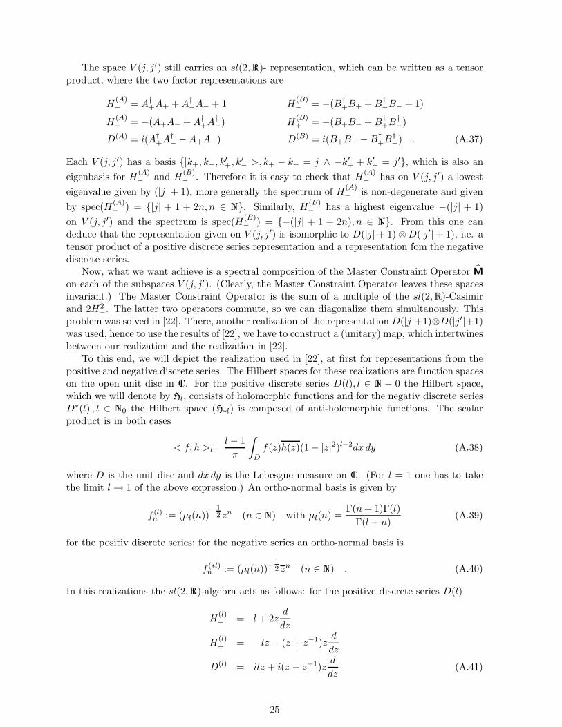
The space V (j, j′) still carries an sl(2,R)- representation, which can be written as a tensorproduct, where the two factor representations are

H(A)− = A†

+A+ +A†−A− + 1 H

(B)− = −(B†

+B+ +B†−B− + 1)

H(A)+ = −(A+A− +A†

+A†−) H

(B)+ = −(B+B− +B†

+B†−)

D(A) = i(A†+A

†− −A+A−) D(B) = i(B+B− −B†

+B†−) . (A.37)

Each V (j, j′) has a basis {|k+, k−, k′+, k′− >, k+ − k− = j ∧ −k′+ + k′− = j′}, which is also an

eigenbasis for H(A)− and H

(B)− . Therefore it is easy to check that H

(A)− has on V (j, j′) a lowest

eigenvalue given by (|j| + 1), more generally the spectrum of H(A)− is non-degenerate and given

by spec(H(A)− ) = {|j| + 1 + 2n, n ∈ N}. Similarly, H

(B)− has a highest eigenvalue −(|j| + 1)

on V (j, j′) and the spectrum is spec(H(B)− ) = {−(|j| + 1 + 2n), n ∈ N}. From this one can

deduce that the representation given on V (j, j′) is isomorphic to D(|j| + 1) ⊗D(|j′| + 1), i.e. atensor product of a positive discrete series representation and a representation fom the negativediscrete series.

Now, what we want achieve is a spectral composition of the Master Constraint Operator M

on each of the subspaces V (j, j′). (Clearly, the Master Constraint Operator leaves these spacesinvariant.) The Master Constraint Operator is the sum of a multiple of the sl(2,R)-Casimirand 2H2

−. The latter two operators commute, so we can diagonalize them simultanously. Thisproblem was solved in [22]. There, another realization of the representation D(|j|+1)⊗D(|j′ |+1)was used, hence to use the results of [22], we have to construct a (unitary) map, which intertwinesbetween our realization and the realization in [22].

To this end, we will depict the realization used in [22], at first for representations from thepositive and negative discrete series. The Hilbert spaces for these realizations are function spaceson the open unit disc in C. For the positive discrete series D(l), l ∈ N − 0 the Hilbert space,which we will denote by Hl, consists of holomorphic functions and for the negativ discrete seriesD∗(l) , l ∈ N0 the Hilbert space (H∗l) is composed of anti-holomorphic functions. The scalarproduct is in both cases

< f, h >l=l − 1

π

∫

Df(z)h(z)(1 − |z|2)l−2dx dy (A.38)

where D is the unit disc and dx dy is the Lebesgue measure on C. (For l = 1 one has to takethe limit l → 1 of the above expression.) An ortho-normal basis is given by

f (l)n := (µl(n))−

12 zn (n ∈ N) with µl(n) =

Γ(n+ 1)Γ(l)

Γ(l + n)(A.39)

for the positiv discrete series; for the negative series an ortho-normal basis is

f (∗l)n := (µl(n))−

12 zn (n ∈ N) . (A.40)

In this realizations the sl(2,R)-algebra acts as follows: for the positive discrete series D(l)

H(l)− = l + 2z

d

dz

H(l)+ = −lz − (z + z−1)z

d

dz

D(l) = ilz + i(z − z−1)zd

dz(A.41)

25

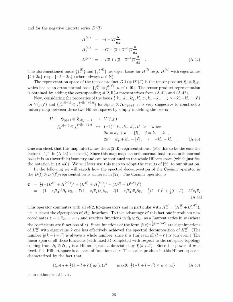
and for the negative discrete series D∗(l)

H(∗l)− = −l− 2z

d

dz

H(∗l)+ = −lz + (z + z−1)z

d

dz

D(∗l) = −ilz + i(z − z−1)zd

dz. (A.42)

The aforementioned bases {f (l)n } and {f (∗l)

n } are eigen-bases for H(l)− resp. H

(∗l)− with eigenvalues

{l + 2n} resp. {−l − 2n} (where always n ∈ N).The representation space of the tensor product D(l)⊗D∗(l′) is the tensor product Hl ⊗H∗l′ ,

which has as an ortho-normal basis {f (l)n ⊗ f

(∗l′)n′ , n, n′ ∈ N}. The tensor product representation

is obtained by adding the corresponding sl(2,R)-representatives from (A.41) and (A.42).Now, considering the properties of the bases {|k+, k−, k′+, k

′− >, k+−k− = j ∧−k′++k′− = j′}

for V (j, j′) and {f (|j|+1)n ⊗ f

(∗(|j′|+1))n′ } for H|j|+1 ⊗ H∗(|j′|+1) it is very suggestive to construct a

unitary map between these two Hilbert spaces by simply matching the bases:

U : H|j|+1 ⊗ H∗(|j′|+1) → V (j, j′)

f (|j|+1)n ⊗ f

(∗(|j′|+1))n′ 7→ (−1)n

′ |k+, k−, k′+, k

′− > where

2n = k+ + k− − |j| , j = k+ − k− ,

2n′ = k′+ + k′− − |j′| , j = −k′+ + k′− . (A.43)

One can check that this map intertwines the sl(2,R)-representations. (For this to be the case thefactor (−1)n

′in (A.43) is needed.) Since this map maps an orthonormal basis to an orthonormal

basis it is an (invertible) isometry and can be continued to the whole Hilbert space (which justifiesthe notation in (A.43)). We will later use this map to adopt the results of [22] to our situation.

In the following we will sketch how the spectral decomposition of the Casimir operator inthe D(l) ⊗D∗(l′)-representation is achieved in [22]. The Casimir operator is

C = 14(−(H

(l)− +H

(∗l′)− )2 + (H

(l)+ +H

(∗l′)+ )2 + (D(l) +D(∗l′))2)

= −(1 − z1z2)2∂z1∂z2 + l′(1 − z1z2)z1∂z1 + l(1 − z1z2)z2∂z2 − 1

4(l − l′)2 + 12(l + l′) − l l′z1z2 .

(A.44)

This operator commutes with all sl(2,R)-generators and in particular with H ll′− = (H

(l)− +H

(∗l′)− ),

i.e. it leaves the eigenspaces of H ll′− invariant. To take advantage of this fact one introduces new

coordinates z = z1z2 , w = z1 and rewrites functions in Hl ⊗H∗l′ as a Laurent series in w (where

the coefficients are functions of z). Since functions of the form f(z)w12 (k−l+l′) are eigenfunctions

of H ll′− with eigenvalue k one has effectively achieved the spectral decomposition of H ll′

− . (Thenumber 1

2(k − l+ l′) is always a whole number, since k is (un)even iff (l − l′) is (un)even.) Thelinear span of all these functions (with fixed k) completed with respect to the subspace-topologycoming from Hl ⊗ H∗l′) is a Hilbert space, abbreviated by H(k, l, l′). Since the power of w isfixed, this Hilbert space is a space of functions of z. The scalar product in this Hilbert space ischaracterized by the fact that

{(µl(n+ 12 (k − l + l′))µl′(n)zn | max(0, 1

2 (−k + l − l′) ≤ n <∞} (A.45)

is an orthonormal basis.

26

One can restrict the Casimir (A.44) to this Hilbert space (since it leaves the H ll′− -eigenspaces

invariant) obtaining

Ck = (1 − z)

(− z(1 − z)

d2

dz2− 1

2(k − l + l′ + 2 − (k + l + 3l′ + 2)z)d

dz+

12 l

′ (k + l + l′) + 14(l + l′)(2 − l − l′)(1 − z)−1

). (A.46)

Likewise the Master Constraint Operator restricts to H(k, l, l′) and can be written as

Mk = 4Ck + 2k2 . (A.47)

These operators are ordinary second order differenential operators and their spectral decompo-sition is effected in [22] by using (modifications of) the Rellich-Titchmarsh-Kodaira-theory. Wewill not explain this procedure but merely cite the results.

The eigenvalue equation for the master constraint (Mk − λ)f = 0 on H(k, l = |j| + 1, l′ =|j′|+ 1) has two linearly independent solutions (since it is a second order differential operator),a near z = 0 regular solution being

fk,j,j′(z, t) = (1 − z)1−t− 12(|j|+|j′|+2)F (1 − t+ 1

2(−|j| + |j′|), 1 − t+ 12k, 1 + 1

2(k − |j| + |j′|); z)(A.48)

for k − |j| + |j′| ≥ 0 and

fk,j,j′(z, t) = (1 − z)1−t− 12(|j|+|j′|+2)z

12(−k+|j|−|j′|) ×

×F (1 − t− 12k, 1 − t+ 1

2(|j| − |j′|), 1 + 12(−k + |j| − |j′|); z) (A.49)

for k − |j| + |j′| ≤ 0, where t = 12(1 +

√1 − λ+ 2k2), Re(t) ≥ 1

2 and F (a, b, c; z) is the hyper-geometric function. For λ(k, |j|, |j′ |) in the spectrum of the Master Constraint Operator thesesolutions are generalized eigenvectors of the Master Constraint Operator.

The spectrum has a continuous part and a discrete part. There is a discrete part only ifk > 0 for |j| − |j′| ≥ 2 or k < 0 for |j| − |j′| ≤ 2.:

λdiscr = 4t(1 − t) + 2k2 ≥ 2k2 − k2 + 2|k|with t = 1, 2, . . . , 1

2min(|k|, ||j| − |j′||) for even k

with t = 32 ,

52 . . . ,

12min(|k|, ||j| − |j′||) for odd k

and (A.50)

λcont = 1 + x2 + 2k2 > 0 x ∈[0,∞

). (A.51)

The spectral resolution of a function f(z) in H(k, l = |j|+1, l′ = |j|+1) is for k−|j|+ |j′| ≥ 0

f(z) =∑

λdiscr

A(λdiscr) +

∫ 12+i∞

12

(2t− 1)µ(j, j′, k, t) < f, fk,j,j′(·, t) > fk,j,j′(z, t) dt

µ(j, j′, k, t) =1

iπ2Γ(|j| + 1)Γ(|j′| + 1)Γ2(12(k − |j| + |j′| + 2))

sinπt cos πt ×

× |Γ(t+ 12k)Γ(t− 1

2(2 − |j| − |j′|))|2|Γ(t− 12(|j| − |j′|))|2 (A.52)

and for k − |j| + |j′| ≤ 0

f(z) =∑

λdiscr

B(λdiscr) +

∫ 12+i∞

12

(2t− 1)µ(j, j′, k, t) < f, fk,j,j′(·, t) > fk,j,j′(z, t) dt

µ(j, j′, k, t) =1

iπ2Γ(|j| + 1)Γ(|j′| + 1)Γ2(12 (−k + |j| − |j′| + 2))

sinπt cos πt ×

× |Γ(t− 12k)Γ(t− 1

2 (2 − |j| − |j′|))|2|Γ(t+ 12(|j| − |j′|))|2 (A.53)

27

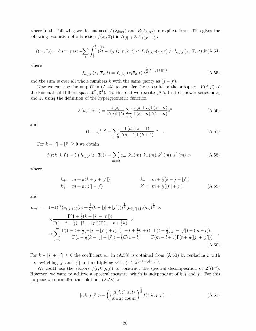
where in the following we do not need A(λdiscr) and B(λdiscr) in explicit form. This gives thefollowing resolution of a function f(z1, z2) in H|j|+1 ⊗ H∗(|j′|+1)):

f(z1, z2) = discr. part +∑

k

∫ 12+i∞

12

(2t− 1)µ(j, j′, k, t) < f, fk,j,j′(·, ·, t) > fk,j,j′(z1, z2, t) dt(A.54)

where

fk,j,j′(z1, z2, t) = fk,j,j′(z1z2, t) z12 (k−|j|+|j′|)1 , (A.55)

and the sum is over all whole numbers k with the same parity as (j − j′).Now we can use the map U in (A.43) to transfer these results to the subspaces V (j, j′) of

the kinematical Hilbert space L2(R4). To this end we rewrite (A.55) into a power series in z1and z2 using the definition of the hypergeometric function

F (a, b, c ; z) =Γ(c)

Γ(a)Γ(b)

∑

n=0

Γ(a+ n)Γ(b+ n)

Γ(c+ n)Γ(1 + n)zn (A.56)

and

(1 − z)1−d =∑

n=0

Γ(d+ k − 1)

Γ(d− 1)Γ(k + 1)zk . (A.57)

For k − |j| + |j′| ≥ 0 we obtain

f(t; k, j, j′) = U(fk,j,j′(z1, z2)) =∑

m=0

am |k+(m), k−(m), k′+(m), k′−(m) > (A.58)

where

k+ = m+ 12(k + j + |j′|) k− = m+ 1

2(k − j + |j′|)k′+ = m+ 1

2(|j′| − j′) k′− = m+ 12(|j′| + j′) (A.59)

and

am = (−1)m(µ(|j|+1)(m+1

2(k − |j| + |j′|)))

12 (µ(|j′|+1)(m))

12 ×

× Γ(1 + 12(k − |j| + |j′|))

Γ(1 − t+ 12(−|j| + |j′|))Γ(1 − t+ 1

2k)×

×m∑

l=0

Γ(1 − t+ 12 (−|j| + |j′|) + l)Γ(1 − t+ 1

2k + l)

Γ(1 + 12 (k − |j| + |j′|) + l)Γ(1 + l)

Γ(t+ 12(|j| + |j′|) + (m− l))

Γ(m− l + 1)Γ(t+ 12 (|j| + |j′|)) .

(A.60)

For k − |j| + |j′| ≤ 0 the coefficient am in (A.58) is obtained from (A.60) by replacing k with

−k, switching |j| and |j′| and multiplying with (−1)12 (−k+|j|−|j′|).

We could use the vectors f(t; k, j, j′) to construct the spectral decomposition of L2(R4).However, we want to achieve a spectral measure, which is independent of k, j and j′. For thispurpose we normalize the solutions (A.58) to

|t, k, j, j′ >=

(iµ(j, j′, k, t)sinπt cos πt

)12f(t; k, j, j′) . (A.61)

28

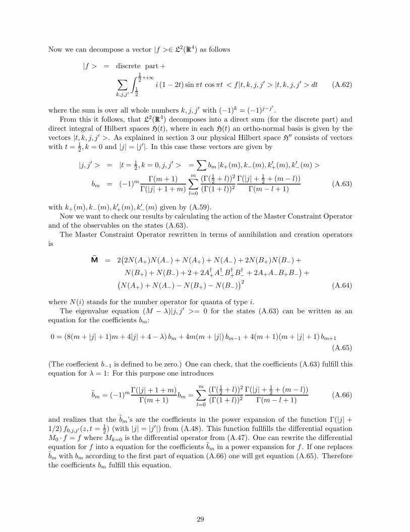
Now we can decompose a vector |f >∈ L2(R4) as follows

|f > = discrete part +

∑

k,j,j′

∫ 12+i∞

12

i (1 − 2t) sinπt cos πt < f |t, k, j, j′ > |t, k, j, j′ > dt (A.62)

where the sum is over all whole numbers k, j, j′ with (−1)k = (−1)j−j′ .From this it follows, that L2(R4) decomposes into a direct sum (for the discrete part) and

direct integral of Hilbert spaces H(t), where in each H(t) an ortho-normal basis is given by thevectors |t, k, j, j′ >. As explained in section 3 our physical Hilbert space H′′ consists of vectorswith t = 1

2 , k = 0 and |j| = |j′|. In this case these vectors are given by

|j, j′ > = |t = 12 , k = 0, j, j′ > =

∑bm |k+(m), k−(m), k′+(m), k′−(m) >

bm = (−1)mΓ(m+ 1)

Γ(|j| + 1 +m)

m∑

l=0

(Γ(12 + l))2

(Γ(1 + l))2Γ(|j| + 1

2 + (m− l))

Γ(m− l + 1)(A.63)

with k+(m), k−(m), k′+(m), k′−(m) given by (A.59).Now we want to check our results by calculating the action of the Master Constraint Operator

and of the observables on the states (A.63).The Master Constraint Operator rewritten in terms of annihilation and creation operators

is

M = 2(2N(A+)N(A−) +N(A+) +N(A−) + 2N(B+)N(B−) +

N(B+) +N(B−) + 2 + 2A†+A

†−B

†+B

†− + 2A+A−B+B−

)+

(N(A+) +N(A−) −N(B+) −N(B−)

)2(A.64)

where N(i) stands for the number operator for quanta of type i.The eigenvalue equation (M − λ)|j, j′ >= 0 for the states (A.63) can be written as an

equation for the coefficients bm:

0 = (8(m+ |j| + 1)m+ 4|j| + 4 − λ) bm + 4m(m+ |j|) bm−1 + 4(m+ 1)(m+ |j| + 1) bm+1

(A.65)

(The coeffecient b−1 is defined to be zero.) One can check, that the coefficients (A.63) fulfill thisequation for λ = 1: For this purpose one introduces

bm = (−1)mΓ(|j| + 1 +m)

Γ(m+ 1)bm =

m∑

l=0

(Γ(12 + l))2

(Γ(1 + l))2Γ(|j| + 1

2 + (m− l))

Γ(m− l + 1)(A.66)

and realizes that the bm’s are the coefficients in the power expansion of the function Γ(|j| +1/2) f0,j,j′(z, t = 1

2) (with |j| = |j′|) from (A.48). This function fullfills the differential equationM0 · f = f where Mk=0 is the differential operator from (A.47). One can rewrite the differentialequation for f into a equation for the coefficients bm in a power expansion for f . If one replacesbm with bm according to the first part of equation (A.66) one will get equation (A.65). Thereforethe coefficients bm fulfill this equation.

29

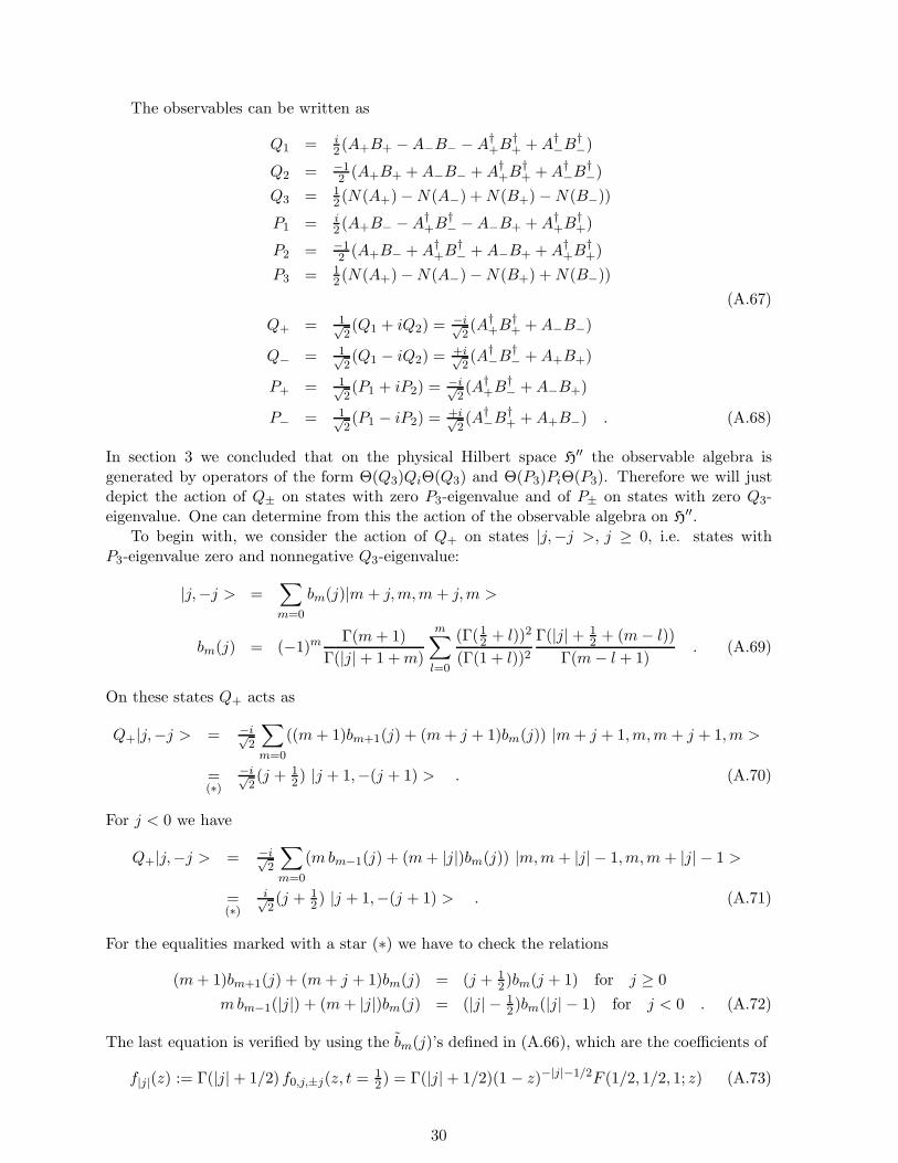
The observables can be written as

Q1 = i2 (A+B+ −A−B− −A†

+B†+ +A†

−B†−)

Q2 = −12 (A+B+ +A−B− +A†

+B†+ +A†

−B†−)

Q3 = 12 (N(A+) −N(A−) +N(B+) −N(B−))

P1 = i2 (A+B− −A†

+B†− −A−B+ +A†

+B†+)

P2 = −12 (A+B− +A†

+B†− +A−B+ +A†

+B†+)

P3 = 12 (N(A+) −N(A−) −N(B+) +N(B−))

(A.67)

Q+ = 1√2(Q1 + iQ2) = −i√

2(A†

+B†+ +A−B−)

Q− = 1√2(Q1 − iQ2) = +i√

2(A†

−B†− +A+B+)

P+ = 1√2(P1 + iP2) = −i√

2(A†

+B†− +A−B+)

P− = 1√2(P1 − iP2) = +i√

2(A†

−B†+ +A+B−) . (A.68)

In section 3 we concluded that on the physical Hilbert space H′′ the observable algebra isgenerated by operators of the form Θ(Q3)QiΘ(Q3) and Θ(P3)PiΘ(P3). Therefore we will justdepict the action of Q± on states with zero P3-eigenvalue and of P± on states with zero Q3-eigenvalue. One can determine from this the action of the observable algebra on H′′.

To begin with, we consider the action of Q+ on states |j,−j >, j ≥ 0, i.e. states withP3-eigenvalue zero and nonnegative Q3-eigenvalue:

|j,−j > =∑

m=0

bm(j)|m + j,m,m+ j,m >

bm(j) = (−1)mΓ(m+ 1)

Γ(|j| + 1 +m)

m∑

l=0

(Γ(12 + l))2

(Γ(1 + l))2Γ(|j| + 1

2 + (m− l))

Γ(m− l + 1). (A.69)

On these states Q+ acts as

Q+|j,−j > = −i√2

∑

m=0

((m+ 1)bm+1(j) + (m+ j + 1)bm(j)) |m+ j + 1,m,m+ j + 1,m >

=(∗)

−i√2(j + 1

2) |j + 1,−(j + 1) > . (A.70)

For j < 0 we have

Q+|j,−j > = −i√2

∑

m=0

(mbm−1(j) + (m+ |j|)bm(j)) |m,m+ |j| − 1,m,m+ |j| − 1 >

=(∗)

i√2(j + 1

2) |j + 1,−(j + 1) > . (A.71)

For the equalities marked with a star (∗) we have to check the relations

(m+ 1)bm+1(j) + (m+ j + 1)bm(j) = (j + 12)bm(j + 1) for j ≥ 0

mbm−1(|j|) + (m+ |j|)bm(j) = (|j| − 12)bm(|j| − 1) for j < 0 . (A.72)

The last equation is verified by using the bm(j)’s defined in (A.66), which are the coefficients of

f|j|(z) := Γ(|j| + 1/2) f0,j,±j(z, t = 12) = Γ(|j| + 1/2)(1 − z)−|j|−1/2F (1/2, 1/2, 1; z) (A.73)

30

in a power expansion in z. Then, rewriting of the identity (1−z)f|j|(z) = (|j|−1/2) f|j|−1(z) into

an equation for the bm(j) and furthermore for the bm(j) results in the last equation of (A.72).For the first equation one starts with the differential equation M0 · f|j|(z) = f|j|(z) and replacesthere (1 − z)−1f|j|(z) with (|j| + 1/2)−1f|j|+1(z). This then translates into the first equation of(A.72) for the coefficients bm(j).

The relations (A.72) will also ensure the following equalities:

Q−|j,−j > = i√2(j − 1

2)|j − 1,−(j − 1) >

P+|j, j > = −i√2(j + 1

2)|j + 1, j + 1 >

P−|j, j > = i√2(j − 1

2)|j − 1, j − 1 > . (A.74)

These formulas differ by phase factors from the formulas in 3.5. One can adjust these phasefactors to one by choosing a new basis |j, ǫj >′= (−i)j |j, ǫj >. Therefore the results of thissection and section 3 are consistent.

References

[1] T. Thiemann, “The Phoenix Project: Master Constraint Programme for Loop QuantumGravity”, gr-qc/0305080

[2] B. Dittrich, T. Thiemann, “Testing the Master Constraint Programme for Loop QuantumGravity I. General Framework”, gr-qc/0411138

[3] B. Dittrich, T. Thiemann, “Testing the Master Constraint Programme for Loop QuantumGravity II. Finite Dimensional Systems”, gr-qc/0411139

[4] B. Dittrich, T. Thiemann, “Testing the Master Constraint Programme for Loop QuantumGravity IV. Free Field Theories”, gr-qc/0411141

[5] B. Dittrich, T. Thiemann, “Testing the Master Constraint Programme for Loop QuantumGravity V. Interacting Field Theories”, gr-qc/0411142

[6] C. Rovelli, “Loop Quantum Gravity”, Living Rev. Rel. 1 (1998) 1, gr-qc/9710008T. Thiemann,“Lectures on Loop Quantum Gravity”, Lecture Notes in Physics, 631 (2003)41 – 135, gr-qc/0210094A. Ashtekar, J. Lewandowski, “Background Independent Quantum Gravity: A Status Re-port”, Class. Quant. Grav. 21 (2004) R53; [gr-qc/0404018]L. Smolin, “An Invitation to Loop Quantum Gravity”, hep-th/0408048

[7] C. Rovelli, “Quantum Gravity”, Cambridge University Press, Cambridge, 2004[8] T. Thiemann, “Modern Canonical Quantum General Relativity”, Cambridge University

Press, Cambridge, 2005, gr-qc/0110034[9] T. Thiemann, “Anomaly-free Formulation of non-perturbative, four-dimensional Lorentzian

Quantum Gravity”, Physics Letters B380 (1996) 257-264, [gr-qc/9606088]T. Thiemann, “Quantum Spin Dynamics (QSD)”, Class. Quantum Grav. 15 (1998) 839-73, [gr-qc/9606089]; “II. The Kernel of the Wheeler-DeWitt Constraint Operator”, Class.Quantum Grav. 15 (1998) 875-905, [gr-qc/9606090]; “III. Quantum Constraint Algebraand Physical Scalar Product in Quantum General Relativity”, Class. Quantum Grav.15 (1998) 1207-1247, [gr-qc/9705017]; “IV. 2+1 Euclidean Quantum Gravity as a modelto test 3+1 Lorentzian Quantum Gravity”, Class. Quantum Grav. 15 (1998) 1249-1280,[gr-qc/9705018]; “V. Quantum Gravity as the Natural Regulator of the Hamiltonian Con-straint of Matter Quantum Field Theories”, Class. Quantum Grav. 15 (1998) 1281-1314,[gr-qc/9705019]; “VI. Quantum Poincare Algebra and a Quantum Positivity of EnergyTheorem for Canonical Quantum Gravity”, Class. Quantum Grav. 15 (1998) 1463-1485,[gr-qc/9705020]; “Kinematical Hilbert Spaces for Fermionic and Higgs Quantum Field The-ories”, Class. Quantum Grav. 15 (1998) 1487-1512, [gr-qc/9705021]

31

[10] A. Ashtekar, J. Lewandowski, D. Marolf, J. Mourao, T. Thiemann, “Quantization for dif-feomorphism invariant theories of connections with local degrees of freedom”, Journ. Math.Phys. 36 (1995) 6456-6493, [gr-qc/9504018]

[11] H. Sahlmann, “When do Measures on the Space of Connections Support the Triad Opera-tors of Loop Quantum Gravity?”, gr-qc/0207112; “Some Comments on the RepresentationTheory of the Algebra Underlying Loop Quantum Gravity”, gr-qc/0207111H. Sahlmann, T. Thiemann, “On the Superselection Theory of the Weyl Algebra for Dif-feomorphism Invariant Quantum Gauge Theories”, gr-qc/0302090; “Irreducibility of theAshtekar-Isham-Lewandowski Representation”, gr-qc/0303074A. Okolow, J. Lewandowski, “Diffeomorphism Covariant Representations of the HolonomyFlux Algebra”, gr-qc/0302059

[12] D. Giulini, D. Marolf , “A Uniqueness Theorem for Constraint Quantization” Class. Quant.Grav. 16:2489-2505,1999, [gr-qc/9902045]; “On the Generality of Refined Algebraic Quan-tization”, Class. Quant. Grav. 16:2479-2488,1999, [gr-qc/9812024]

[13] J. Klauder, “Universal Procedure for Enforcing Quantum Constraints”,Nucl.Phys.B547:397-412,1999, [hep-th/9901010]; “Quantization of Constrined Sys-tems”, Lect. Notes Phys. 572 (2001) 143-182, [hep-th/0003297]A. Kempf, J. Klauder, “On the Implementation of Constraints through ProjectionOperators”, J. Phys. A34 (2001) 1019-1036, [quant-ph/0009072]

[14] T. Thiemann, “Quantum Spin Dynamics (QSD): VIII. The Master Constraint”, in prepa-ration

[15] H. Sahlmann, T. Thiemann, “Towards the QFT on Curved Spacetime Limit of QGR. 1. AGeneral Scheme”, [gr-qc/0207030]; “2. A Concrete Implementation”, [gr-qc/0207031]

[16] T. Thiemann, “Quantum Spin Dynamics (QSD): VII. Symplectic Structures and Contin-uum Lattice Formulations of Gauge Field Theories”, Class.Quant.Grav.18:3293-3338,2001,[hep-th/0005232]; “Gauge Field Theory Coherent States (GCS): I. General Properties”,Class.Quant.Grav.18:2025-2064,2001, [hep-th/0005233]; “Complexifier Coherent States forCanonical Quantum General Relativity”, gr-qc/0206037T. Thiemann, O. Winkler, “Gauge Field Theory Coherent States (GCS): II. PeakednessProperties”, Class.Quant.Grav.18:2561-2636,2001, [hep-th/0005237]; “III. Ehrenfest Theo-rems”, Class. Quantum Grav. 18 (2001) 4629-4681, [hep-th/0005234]; “IV. Infinite Ten-sor Product and Thermodynamic Limit”, Class. Quantum Grav. 18 (2001) 4997-5033,[hep-th/0005235]H. Sahlmann, T. Thiemann, O. Winkler, “Coherent States for Canonical Quantum Gen-eral Relativity and the Infinite Tensor Product Extension”, Nucl.Phys.B606:401-440,2001[gr-qc/0102038]

[17] M. Reed, B. Simon, “Functional Analysis”, vol. 1, Academic Press, New York, 1980[18] A. Paterson, “Amenability”, American Mathematical Society, Providence, Rhode Island,

1988J.P. Pier, “Amenable Locally Compact Groups”, New York, Wiley, 1984A. Carey, H. Grundling, “Amenability of the Gauge Group”, math-ph/0401031

[19] R. Howe, E.C. Tan, “Non-Abelian Harmonic Analysis – Applications of SL(2,R)”, (Springer,New-York,1992)

[20] R. Howe, “On some results of Strichartz and of Rallis and Schiffman”, J. Funct. Anal.32,297 (1979)

[21] R. Howe, “Dual pairs in physics: Harmonic oscillators, photons, electrons, and singletons”,Lectures in Appl. Math., Vol. 21, pp.275-286, Amer. Math. Soc., Providence, RI, 1979

[22] H. Neunhoffer, “Uber Kronecker-Produkte irreduzibler Darstellungen von SL(2,R)”,Sitzungsberichte der Heidelberger Akademie der Wissenschaften, Mathematisch-naturwissenschaftliche Klasse, Jahrgang 1978, 167

32

[23] M. Montesinos, C. Rovelli, T. Thiemann, “SL(2,R) model with two Hamiltonian con-straints”, Phys. Rev. D60,044009 (1999), gr-qc/9901073

[24] J. Louko, C. Rovelli, “Refined algebraic quantization in the oscillator representation ofSL(2,R)”, J. Math. Phys. 41, 132 (2000), gr-qc/9907004

[25] J. Louko, A. Molgado, “Group averaging in the (p, q) oscillator representation ofSL(2,R)”,J. Math. Phys. 45 1919 (2004), gr-qc/0312014

[26] M. Trunk, ”An “SL(2,R) model of constrained systems: Algebraic constrained quantiza-tion”, University of Freiburg preprint THEP 99/3, hep-th/9907056

[27] R. Gambini, R.A. Porto, “Relational time in generally covariant quantum systems: Fourmodels”, Phys. Rev. D63, 105014 (2001), gr-qc/0101057

[28] J. Repka, “Tensor products of unitary representations of SL(2,R)”, Amer. J. Math. 100(4),747 (1978)

[29] A. Gomberoff, D. Marolf, “On Group Averaging for SO(n, 1)”,Int. J. Mod. Phys. D8, 519(1999), gr-qc/9902069

[30] B.G. Adams, J. Cizek, J. Paldus, “Lie Algebraic Methods and Their Applications to SimpleQuantum Systems”, Adv. Quantum Chem. 19, 1 (1988)

[31] V. Bargmann, “Irreducible unitary representations of the Lorentz group”, Ann. of Math.48, 568 (1947)

33