Testing of Photomultiplier Tubes for Use in the Surface ... · Testing of Photomultiplier Tubes for...

Testing of Photomultiplier Tubes for Use in

the Surface Detector of the Pierre Auger

Observatory

D. Barnhill a,∗, F. Suarez b,∗, K. Arisaka a, B. Garcia c,

J. P. Gongora d, A. Lucero c, I. Navarro c, T. Ohnuki a, A. Risi d,A. Tripathi a

aDepartment of Physics and Astronomy, UCLA, Los Angeles, CA 90095-1547bINFN, Universita degli Studi di Torino, Italia

cUTN-FRM Mendoza, ArgentinadUTN-FRSR San Rafael, Argentina

Abstract

In the array of water Cherenkov detectors of the Pierre Auger Observatory, 4800large photomultiplier tubes (PMTs) will be used. Before being deployed, each PMTis evaluated to check that various parameters, such as the linearity, dark noise, andgain, fall within a specified range. The large scale test system, designed and con-structed for this purpose, is capable of testing multiple large PMTs simultaneously.The test system and the results of the tests for the first 3964 PMTs are presentedin this paper.

Key words: PMTs; Photodetectors; Water Cherenkov; Cosmic Rays; AstroparticlePhysics; Pierre Auger

1 Introduction1

The Pierre Auger Observatory, currently being constructed in the province2

of Mendoza in Argentina, is designed to measure the energies, directions, and3

∗ Corresponding author.Email addresses: [email protected] (D. Barnhill),

[email protected] (F. Suarez).

Preprint submitted to Elsevier Science 22 March 2007

composition of the highest energy cosmic rays arriving at the earth. To accom-4

plish this task, the observatory will be comprised of two detectors: a surface5

detector, which is an array of 1600 water Cherenkov detectors deployed over6

∼3000 km2, and 24 fluorescence telescopes grouped into 4 sites, which over-7

look the surface detector [1]. Being able to measure ultra high energy cosmic8

rays using both techniques will provide unprecedented information about the9

nature and origin of these particles.10

However, the Auger Observatory can only operate in “hybrid” mode (or using11

both the fluorescence and surface detectors together) ∼10% of the time [2]. The12

remaining 90% of the time, the surface detector operates alone. It is critical,13

then, that the surface detector is well understood as it is the foundation for14

all of the data taken at the Auger Observatory.15

The surface detector is made up of an array of water Cherenkov detectors, or16

stations, which are cylindrical water tanks, 3.6 m in diameter and 1.2 m deep.17

They are filled with purified water and have a reflective interior that is fitted18

with 3 × 9” Photonis XP1805 PMTs which look down into the station. The19

PMTs are equipped with a resistive base and a local High Voltage module [3].20

When a relativistic particle enters the station, it emits Cherenkov radiation21

that propagates through the water, being reflected at the station walls until22

it is either absorbed or detected by the PMTs.23

When completed, the surface detector will have 1600 stations, which will em-24

ploy the use of 4800 PMTs. Including spares, the Auger Observatory will25

receive more than 5000 PMTs for use in the surface detector, and it is the26

testing and characterization of these PMTs that is addressed in this paper.27

The layout of the paper is as follows: first, in Section 2, the test system will28

be described, including the hardware that was designed specifically for this29

system. Then, the tests run on the PMTs along with the results of testing will30

be presented. Finally, in Section 3, the monitoring of the test system will be31

described with a discussion of the results.32

2 Testing of Photomultiplier Tubes33

The purpose of testing each PMT before being deployed is two-fold. The tests34

are to verify that each PMT is within the specifications given to Photonis,35

specifications that are designed to ensure that only PMTs of the desired quality36

are used in the surface detector, resulting in uniform behavior across the array37

of stations. Secondly, we are able to give valuable feedback to the company38

regarding the performance of the PMTs which they can use to improve their39

product.40

2

Test Specification

SPE Peak to Valley >1.2

Gain versus Voltage 106 gain with V< 2000 Volts

Dark Pulse Rate < 10 kHz at 1/4 pe threshold

Non-linearity < 6% below 50 mA peak current

Dynode to Anode Ratio between 25 and 40

Afterpulse Ratio < 5%

Table 1Specifications to determine if a PMT passed or failed a given test.

The specifications regarding the performance of the PMTs to be used in the41

surface detector is driven by the physics that is being done. It is desirable to42

have PMTs with a large dynamic range, good linearity, low counting rate, and43

low background. Because the calibration of the surface detector is done using44

atmospheric muons rather than depending on a knowledge of the absolute45

gain of each PMT, the desired energy resolution is not strictly specified. In46

Table 1 the specifications are listed to determine which PMTs will be used in47

the surface detector and are adapted from the original specifications given in48

Tripathi et al. [4], where PMTs from different companies were compared and49

analyzed as to which would best suit the needs of the Auger Observatory.50

To illustrate the relationship between the specifications and the physics done51

with the Auger Observatory, we consider the calculation of the primary energy52

of a cosmic ray. As a first step, the energy deposited in each station involved53

in the air-shower must be known. The calibration of each station is done using54

single muons which are constantly passing through it [5], while a cosmic ray air-55

shower may cause tens of thousands of particles to enter a given station during56

1 microsecond. Therefore, it is desirable to have PMTs which have a linear57

response over this large dynamic range. The non-linearity test specification58

(less than 6% non-linearity below 50 mA, see Table 1), is designed to reject59

PMTs which deviate from linearity over this range. Related to this issue is60

the afterpulse measurement, as any afterpulsing in the PMTs may lead to a61

miscalculation of the energy deposited in a station.62

To cover the dynamic range of physical signals, from single muons to tens of63

thousands of particles, the output of the last dynode before the anode is tapped64

and amplified [3]. The amplified signal from the dynode makes it possible for65

the station to be triggered by single muons passing through a station, while66

the signal from the anode is used for the detection of any signal that saturates67

the readout electronics of the amplified dynode. Therefore, the ratio of the68

signal from the dynode to the signal from the anode must be known and the69

overall gain of the dynode chain must fall within a specific range. The absolute70

gain as a function of input voltage is measured using a single photoelectron71

3

CAMAC

HV Control

BoxControlLightDAQ Computer

4 LED Pulsers

Dark Room

16 PMTsADC

ADC

ADC

LeCroy 2249

Buffer

TRIGGER

ANALOG BRIGHTNESS

Digital: 4 off/on + Trigger

DYNODE

ANODE

10 Ω

510 Ω

510 Ω50 Ω

Fig. 1. Layout of the PMT data acquisition system.

spectrum. The PMTs and bases were designed to operate with a gain between72

2 × 105 and 106, and are currently being operated at ∼3 × 105 gain [5]. All73

tests are explained in more detail in Section 2.2, but first, the design of the74

test system itself is described.75

2.1 The Test System76

The system is designed to test 16 PMTs in a single run (see Figures 1 and 2).77

However, to monitor the stability of the system, there are 4 permanent PMTs78

located at the corners of the test stand. These PMTs monitor the stability of79

the light source as well as the readout electronics and the performance of the80

system overall. Each test run lasts about 5 hours and is completely automated.81

This makes it possible to do 2 test runs per day resulting in 24 PMTs per day82

being tested.83

The entire test system is controlled with the data acquisition (DAQ) computer,84

see Fig. 1. This computer controls the voltages delivered to the 16 PMTs via85

a High Voltage (HV) Box, controls the intensity and the firing of 4 LEDs (386

blue and 1 UV) through the Light Control Box and LED Pulsers, and controls87

the signal which triggers the camac data acquisition system.88

4

Fig. 2. Top: PMTs in the dark room. Bottom: The data acquisition system with thecamac crate and custom electronics in the rack on the left.

5

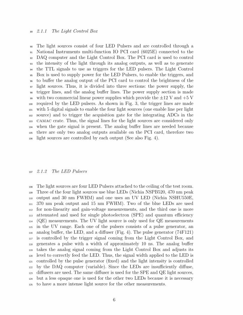
2.1.1 The Light Control Box89

The light sources consist of four LED Pulsers and are controlled through a90

National Instruments multi-function IO PCI card (6025E) connected to the91

DAQ computer and the Light Control Box. The PCI card is used to control92

the intensity of the light through its analog outputs, as well as to generate93

the TTL signals to use as triggers for the LED pulsers. The Light Control94

Box is used to supply power for the LED Pulsers, to enable the triggers, and95

to buffer the analog output of the PCI card to control the brightness of the96

light sources. Thus, it is divided into three sections: the power supply, the97

trigger lines, and the analog buffer lines. The power supply section is made98

with two commercial linear power supplies which provide the ±12 V and +5 V99

required by the LED pulsers. As shown in Fig. 3, the trigger lines are made100

with 5 digital signals to enable the four light sources (one enable line per light101

source) and to trigger the acquisition gate for the integrating ADCs in the102

camac crate. Thus, the signal lines for the light sources are considered only103

when the gate signal is present. The analog buffer lines are needed because104

there are only two analog outputs available on the PCI card, therefore two105

light sources are controlled by each output (See also Fig. 4).106

2.1.2 The LED Pulsers107

The light sources are four LED Pulsers attached to the ceiling of the test room.108

Three of the four light sources use blue LEDs (Nichia NSPB520, 470 nm peak109

output and 30 nm FWHM) and one uses an UV LED (Nichia NSHU550E,110

370 nm peak output and 15 nm FWHM). Two of the blue LEDs are used111

for non-linearity and gain-voltage measurements, and the third one is more112

attenuated and used for single photoelectron (SPE) and quantum efficiency113

(QE) measurements. The UV light source is only used for QE measurements114

in the UV range. Each one of the pulsers consists of a pulse generator, an115

analog buffer, the LED, and a diffuser (Fig. 4). The pulse generator (74F121)116

is controlled by the trigger signal coming from the Light Control Box, and117

generates a pulse with a width of approximately 10 ns. The analog buffer118

takes the analog signal coming from the Light Control Box and adjusts its119

level to correctly feed the LED. Thus, the signal width applied to the LED is120

controlled by the pulse generator (fixed) and the light intensity is controlled121

by the DAQ computer (variable). Since the LEDs are insufficiently diffuse,122

diffusers are used. The same diffuser is used for the SPE and QE light sources,123

but a less opaque one is used for the other two LEDs because it is necessary124

to have a more intense light source for the other measurements.125

6

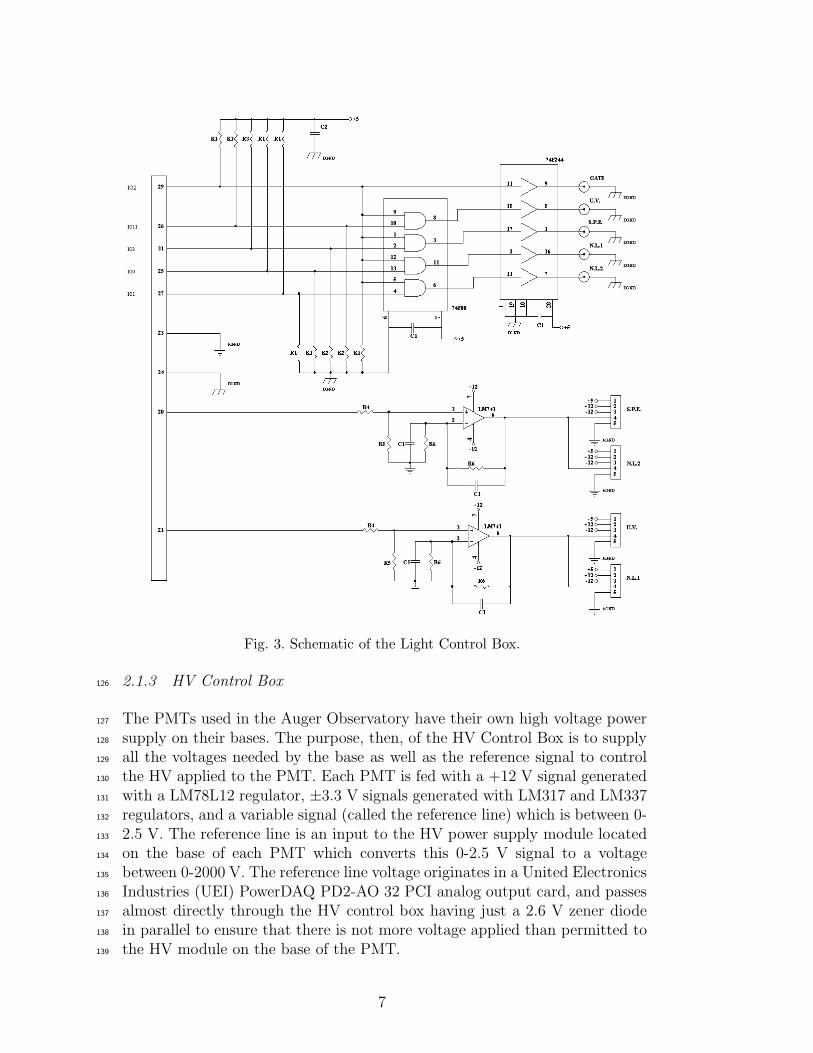
Fig. 3. Schematic of the Light Control Box.

2.1.3 HV Control Box126

The PMTs used in the Auger Observatory have their own high voltage power127

supply on their bases. The purpose, then, of the HV Control Box is to supply128

all the voltages needed by the base as well as the reference signal to control129

the HV applied to the PMT. Each PMT is fed with a +12 V signal generated130

with a LM78L12 regulator, ±3.3 V signals generated with LM317 and LM337131

regulators, and a variable signal (called the reference line) which is between 0-132

2.5 V. The reference line is an input to the HV power supply module located133

on the base of each PMT which converts this 0-2.5 V signal to a voltage134

between 0-2000 V. The reference line voltage originates in a United Electronics135

Industries (UEI) PowerDAQ PD2-AO 32 PCI analog output card, and passes136

almost directly through the HV control box having just a 2.6 V zener diode137

in parallel to ensure that there is not more voltage applied than permitted to138

the HV module on the base of the PMT.139

7

Fig. 4. Schematic of the LED Pulsers.

This box also provides an interlock system that requires the door of the dark140

room to be closed and the key to be inserted into the HV Control Box, which141

also automatically turns off the lights of the test room. If the key is not in the142

HV Control Box, no voltage is supplied to the PMTs. This is needed because143

the PMTs can be seriously damaged if HV is applied when ambient light is144

present.145

2.1.4 The Splitter146

For certain measurements, the dynamic range of the charge-integrating ADC147

modules is insufficient for the desired range of signals. Therefore, the signal148

from the anode is divided into three signals through a resistive splitter (see149

Fig. 5). Thus, two of the outputs from this splitter have approximately 8.5%150

of the charge of the original signal (called the attenuated anode signal), and151

the other output has the remaining 83% (called the anode signal). The atten-152

uated anode signal is used when the anode signal saturates the ADCs. The153

remaining attenuated anode output is used for monitoring purposes, oscillo-154

scope connections, or other measurements.155

2.1.5 PMT Signals and DAQ156

The signals of the PMTs come from two places, the anode as is customary,157

but also from an amplified tap from the last dynode in the amplification chain158

8

Fig. 5. Schematic of the Splitter.

of the PMT. This is done to extend the dynamic range of the PMTs when159

they are in the detectors taking data. To further extend the dynamic range160

of the system for testing purposes, the signal from the anode is broken into161

three components, as explained in the previous section, see Fig. 1. Again, this162

is done to extend the range over which the PMTs can be tested.163

The signals from the PMT are then put into a charge-integrating ADC in a164

camac crate (LeCroy 2249A and 2249W) where they are measured and then165

read out by the DAQ computer. The gate for charge integration is triggered166

by the Light Control Box, but the gate and width are controlled by a camac167

gate-and-delay generator (LeCroy 2323A). All the analysis is then done on the168

DAQ computer.169

2.2 Tests and Results170

Using this test system, 3964 PMTs have been tested out of the 5000 needed171

for the surface detector. The tests run by the system are single photoelectron172

(SPE) spectrum, gain as a function of voltage, dark pulse rate at 1/4 pho-173

toelectron (pe) threshold, non-linearity, dynode to anode ratio, excess noise174

factor, and afterpulse ratio. Each test will be described in greater detail in the175

following sections.176

2.2.1 Single Photoelectron Spectrum177

To obtain the absolute gain of the phototube at a certain voltage, a single178

photoelectron spectrum is measured. This is done by setting the PMT to a179

gain of ∼2 × 106, according to measurements done at Photonis, and flashing180

the LED at an intensity such that 90% of the time there are no photoelectrons181

9

(pe) at the first dynode in the PMT. From Poisson statistics:182

P (n) =e−ννn

n!(1)183

where P (n) is the probability to see exactly n pe, if there are 0 pe 90% of184

the time, then P (0) = e−ν = 0.9, so that ν = 0.105. Then, the probability of185

seeing 1 pe is: P (1) = νe−ν = 0.095, and the probability of seeing more than186

1 is 0.005, or there is a ∼0.5% contamination of events caused by 2 or more187

pe in any given single photoelectron spectrum. The signal then is dominated188

by single photoelectron events, P (1)/P (n > 1) = 21.189

A typical single photoelectron spectrum can be seen in Fig. 6. To calculate the190

gain from this spectrum, the pedestal (or the signal deposited with no light)191

and the standard deviation of the pedestal is established in a measurement192

directly preceding the single photoelectron measurement. Once this is known,193

data are taken with the light source such that 90% of the events are 0 pe194

events. The resulting spectrum contains events from 0 pe, 1 pe, 2 pe, etc. To195

calculate the gain, it is necessary to find the mean of the single pe distribution,196

correcting for 2 pe contamination and compensating for events that are under197

the pedestal.198

To compensate for events under the pedestal, a simple extrapolation of the199

behavior near the pedestal is assumed. Using this extrapolation, the mean of200

the non-zero pe distribution is adjusted. To account for 2 pe events, a correc-201

tion is made utilizing the Poisson nature of the light source. The correction is202

calculated knowing that the mean of the non-zero pe distribution is:203

x =µ1P (1) + µ2P (2) + µ3P (3) + · · ·

P (1) + P (2) + P (3) + · · ·(2)204

where µn is the mean of the n pe distribution and P (n) is the probablity to205

have exactly n pe. Ignoring any events from 3 or more pe and knowing that206

µ2 = 2µ1, equation 2 is solved for µ1, the true mean of the single photoelectron207

spectrum, in terms of x, the mean of the measured distribution:208

µ1 =1 + ν/2

1 + νx (3)209

using ν from equation 1.210

To quantify the resolution of the single photoelectron spectrum, the peak to211

valley ratio is used. The peak to valley ratio is the ratio of the maximum value212

of the histogram of the single photoelectron spectrum to the minimum value213

between the pedestal and the maximum. To calculate this number, smoothing214

10

is done on the distribution, meaning that the value in each bin of the histogram215

is replaced with the average of the current bin with the preceding 2 bins and216

the 3 bins that follow:217

x′

n =xn−2 + xn−1 + · · · + xn+3

6(4)218

One then just steps through the smoothed bins (x′) and finds the minimum219

value (between the pedestal and the mean of the single photoelectron distri-220

bution) and the maximum value of the histogram. The peak to valley ratio of221

the PMT shown in Fig. 6 is 1.47. In Fig. 7, the distribution of peak to valley222

ratios for PMTs tested in the system is shown.223

2.2.2 Gain as a Function of Voltage224

Once the gain is calculated from the SPE spectrum, the absolute gain at that225

voltage is known. However, it is necessary to have several points to determine226

the gain as a function of the input voltage. The relationship between the gain227

and input voltage can be described accurately as a power law:228

G = kV β (5)229

log G = γ + β log V with γ = log k (6)230

with γ and β being parameters to be determined from measurements.231

In the test system, to determine this relationship the LED is pulsed with a232

constant intensity and the PMT is set at different voltages. This determines233

the slope of the relationship between gain and voltage. The value of the gain at234

the voltage used by the SPE measurement is then used as a point that this line235

must pass through. This uniquely determines the two unknown parameters and236

one can calculate the gain of the phototube at any input voltage. An example237

of the gain versus voltage curve is given in Fig. 8, and for this particular PMT,238

γ = -12.190 and β = 5.7562.239

In Fig. 8, the measurements taken at Photonis are shown on the same plot to240

illustrate the difference between two methods of measuring the gain. At Pho-241

tonis, the measurements are made using a constant light source and measuring242

the current of the photocathode and the anode. The gain is then the ratio of243

the anode current to the photocathode current. In this method, the collection244

efficiency (or the percentage of photoelectrons from the photocathode that245

reach the first dynode) is included, whereas, in the SPE method it is not. As246

a result, one can take the ratio of the gain as calculated by the SPE method247

and the gain calculated using the method just described and obtain an esti-248

mate of the collection efficiency at a given voltage. Calculating the collection249

11

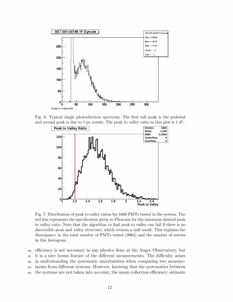
Fig. 6. Typical single photoelectron spectrum. The first tall peak is the pedestaland second peak is due to 1 pe events. The peak to valley ratio in this plot is 1.47.

Entries 3460Mean 1.549RMS 0.2059Underflow 5Overflow 5

Peak to Valley1 1.2 1.4 1.6 1.8 2 2.2 2.40

20

40

60

80

100

120


Peak to Valley Ratio

Fig. 7. Distribution of peak to valley ratios for 3460 PMTs tested in the system. Thered line represents the specification given to Photonis for the minimum desired peakto valley ratio. Note that the algorithm to find peak to valley can fail if there is nodiscernible peak and valley structure, which returns a null result. This explains thediscrepancy in the total number of PMTs tested (3964) and the number of entriesin this histogram.

efficiency is not necessary in any physics done at the Auger Observatory, but250

it is a nice bonus feature of the different measurements. The difficulty arises251

in understanding the systematic uncertainties when comparing two measure-252

ments from different systems. However, knowing that the systematics between253

the systems are not taken into account, the mean collection efficiency estimate254

12

Fig. 8. A typical curve for the gain as a function of voltage for a PMT tested in thesystem, shown with the curve obtained by Photonis.

Photonis Voltage1000 1200 1400 1600 1800 2000

Au

ger

Vo

ltag

e

1000

1200

1400

1600

1800

2000

6Auger vs. Photonis Gain=1x10

Fig. 9. Voltage to get a gain of 106 as measured by our test system (axis labeledAuger Voltage) and Photonis. The red line is the specification given to Photonisand the dashed line is y=x.

is calculated as an exercise and the result is ∼70%. This is calculated at the255

voltage necessary for a gain of 106 using 3933 PMTs.256

Fig. 9 is a plot of the voltage necessary to get a gain of 106 as determined257

by the SPE method (axis labeled Auger Voltage) and using the photocathode258

13

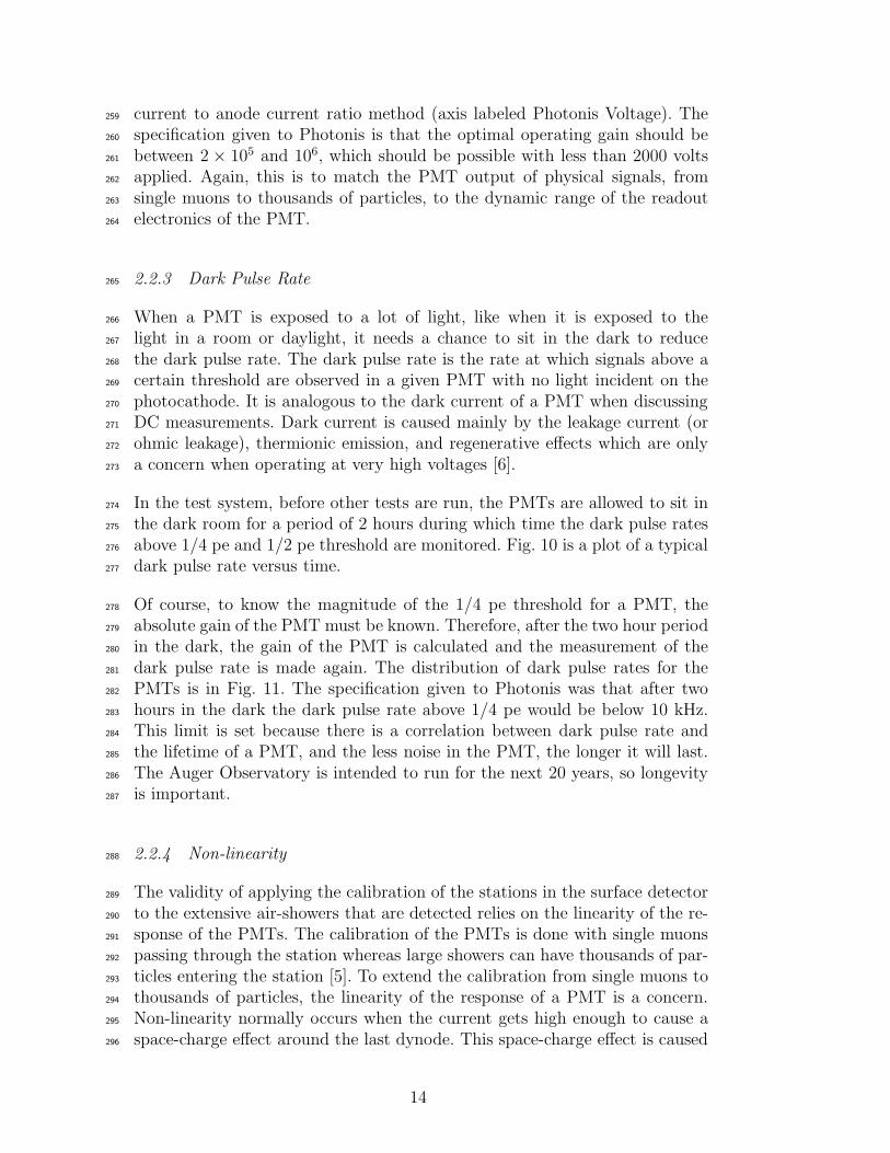
current to anode current ratio method (axis labeled Photonis Voltage). The259

specification given to Photonis is that the optimal operating gain should be260

between 2 × 105 and 106, which should be possible with less than 2000 volts261

applied. Again, this is to match the PMT output of physical signals, from262

single muons to thousands of particles, to the dynamic range of the readout263

electronics of the PMT.264

2.2.3 Dark Pulse Rate265

When a PMT is exposed to a lot of light, like when it is exposed to the266

light in a room or daylight, it needs a chance to sit in the dark to reduce267

the dark pulse rate. The dark pulse rate is the rate at which signals above a268

certain threshold are observed in a given PMT with no light incident on the269

photocathode. It is analogous to the dark current of a PMT when discussing270

DC measurements. Dark current is caused mainly by the leakage current (or271

ohmic leakage), thermionic emission, and regenerative effects which are only272

a concern when operating at very high voltages [6].273

In the test system, before other tests are run, the PMTs are allowed to sit in274

the dark room for a period of 2 hours during which time the dark pulse rates275

above 1/4 pe and 1/2 pe threshold are monitored. Fig. 10 is a plot of a typical276

dark pulse rate versus time.277

Of course, to know the magnitude of the 1/4 pe threshold for a PMT, the278

absolute gain of the PMT must be known. Therefore, after the two hour period279

in the dark, the gain of the PMT is calculated and the measurement of the280

dark pulse rate is made again. The distribution of dark pulse rates for the281

PMTs is in Fig. 11. The specification given to Photonis was that after two282

hours in the dark the dark pulse rate above 1/4 pe would be below 10 kHz.283

This limit is set because there is a correlation between dark pulse rate and284

the lifetime of a PMT, and the less noise in the PMT, the longer it will last.285

The Auger Observatory is intended to run for the next 20 years, so longevity286

is important.287

2.2.4 Non-linearity288

The validity of applying the calibration of the stations in the surface detector289

to the extensive air-showers that are detected relies on the linearity of the re-290

sponse of the PMTs. The calibration of the PMTs is done with single muons291

passing through the station whereas large showers can have thousands of par-292

ticles entering the station [5]. To extend the calibration from single muons to293

thousands of particles, the linearity of the response of a PMT is a concern.294

Non-linearity normally occurs when the current gets high enough to cause a295

space-charge effect around the last dynode. This space-charge effect is caused296

14

Fig. 10. Plot of the dark pulse rate versus time spent in the dark room. Open boxesare 1/4 pe threshold while solid boxes are 1/2 pe threshold.


Darkrate (kHz)0 2 4 6 8 10 12 140

100

200

300

400

500


Darkrate (0.25 pe threshold)

Fig. 11. Distribution of dark pulse rates (1/4 pe threshold) after 2 hours in the darkroom. The red line represents the specification given to Photonis. More than 99%of the PMTs pass this specification.

by an excessive amount of electrons which change the electric field in that297

region, causing the normal trajectory of the electrons to be skewed. Thus,298

the amount of electrons arriving at the last dynode, and hence the anode, is299

smaller than expected. This causes a negative non-linearity. In many of the300

PMTs from Photonis, there is a positive non-linearity which is due to the301

design of the dynode chain. It is designed to collect electrons more efficiently302

at higher currents which causes signal to be lost at lower currents. This ap-303

pears as a positive non-linearity due to the definition of non-linearity (see304

15

Fig. 12. Non-linearity versus peak anode current for a typical PMT.

Maximum Positive (%)0 1 2 3 4 5 6 7 8

NL

at

50 m

A (

%)

-8

-6

-4

-2

0

2

4

6

8

Non-linearity

Fig. 13. Non-linearity at 50 mA versus maximum positive non-linearity. The redlines represent the 6% limit given to Photonis and the blue dotted line is y=x. 98%of the PMTs pass this specification.

equation 7).305

The method to measure non-linearity uses two LEDs. LED A is fired, LED306

B is fired, LED A and B are fired simultaneoulsy, then no LED is fired (to307

obtain the baseline or pedestal). The non-linearity is then defined as:308

NL(%) = 100 ×QAB − (QA + QB)

QA + QB

(7)309

16

where QA is the signal from firing LED A alone, QB is the signal from LED B310

alone, and QAB is the signal from firing LED A and B simultaneously (all are311

baseline subtracted). This sequence is repeated at several light intensities to312

map out the non-linearity as a function of peak anode current. A typical non-313

linearity curve is shown in Fig. 12. In this figure, the positive non-linearity314

feature is evident as well as the following negative non-linearity due to the315

space-charge effect.316

To illustrate the properties of the non-linearity in the PMTs from Photonis,317

a plot of the maximum non-linearity versus the non-linearity at 50 mA is318

shown in Fig. 13. The reason 50 mA is chosen is because the specification319

given to Photonis was that the non-linearity be less than ±6% with a peak320

anode current of less than 50 mA. In the original design of the Pierre Auger321

Observatory, this was estimated to be the peak current at 1000 m from the322

core of an air-shower initiated by a cosmic ray with an energy of 1021 eV [7].323

In Fig. 13, it is evident that almost all the PMTs have a positive non-linearity,324

and the maximum positive non-linearity often occurs around 50 mA of peak325

anode current. It should be noted that the maximum positive non-linearity326

is defined as the maximum non-linearity with a peak anode current less than327

50 mA. If non-linearity continues to increase after a current of 50 mA, that328

is not considered in the definition of maximum positive non-linearity, which329

is why there are no points above the blue dotted line in Fig. 13. Recently,330

Photonis has improved the linearity of the PMTs to eliminate the positive331

non-linearity effect. Results from the first batches of the new PMTs indicate332

that the mean value of the maximum positive non-linearity is less than 1%, and333

this change does not affect the acceptable behavior of the other characteristics334

of the PMTs.335

2.2.5 Dynode to Anode Ratio336

To enable the detection of small signals in the water Cherenkov detectors and337

extend the dynamic range of the detector, the signal from the last dynode is338

extracted and amplified. The amplification is fixed via the electronics on the339

base of the PMT to be a factor of 40. There are then two signals from the340

PMT, the amplified dynode and the signal from the anode. As stated before,341

the calibration is done with single muons which give a small signal and are342

recorded using the amplified signal from the dynode. Once a large number of343

particles pass through a station from an air-shower, the dynode reaches the344

maximum dynamic range of the PMT readout electronics and the signal from345

the anode is used in the analysis instead. To be able to extend the calibration346

using muons, which is measured using the signals from the amplified dynode,347

to the signals from an air-shower, recorded using signals from the anode, the348

amplification of the signal from the dynode when compared to the signal from349

17

the anode must be known. This is known as the dynode to anode ratio, and it350

depends on the gain of the last dynode since the amplification of the dynode351

is fixed to a value of 40.352

D/A = α = 40δ − 1

δ(8)353

In equation 8, the relationship between the dynode to anode ratio (α) and354

the gain of the last dynode (δ) is defined. The factor of 40 is the value of the355

gain of the amplifier. The factor of (δ−1)/δ represents that for every electron356

that hits the last dynode, δ electrons leave. This gives a signal of 1− δ on the357

last dynode and δ on the anode (in arbitrary units). The amplifier inverts and358

amplifies the signal from the last dynode to make it the same polarity as the359

anode.360

To measure the dynode to anode ratio, the PMTs are set to a fixed gain and361

the light source is flashed at varying intensities. The signal of the dynode362

versus the signal of the anode is plotted and the slope of the resulting line363

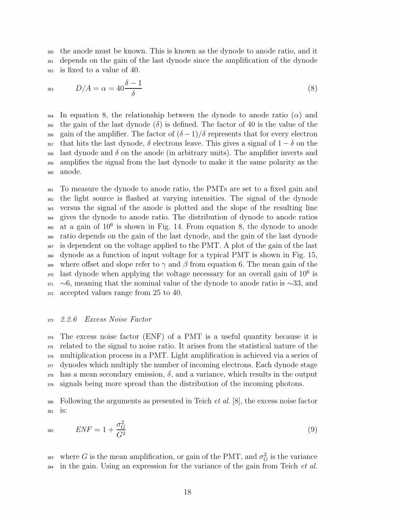
gives the dynode to anode ratio. The distribution of dynode to anode ratios364

at a gain of 106 is shown in Fig. 14. From equation 8, the dynode to anode365

ratio depends on the gain of the last dynode, and the gain of the last dynode366

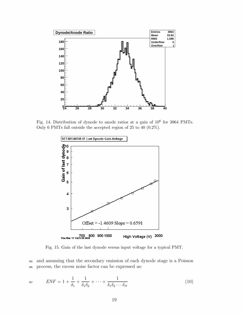
is dependent on the voltage applied to the PMT. A plot of the gain of the last367

dynode as a function of input voltage for a typical PMT is shown in Fig. 15,368

where offset and slope refer to γ and β from equation 6. The mean gain of the369

last dynode when applying the voltage necessary for an overall gain of 106 is370

∼6, meaning that the nominal value of the dynode to anode ratio is ∼33, and371

accepted values range from 25 to 40.372

2.2.6 Excess Noise Factor373

The excess noise factor (ENF) of a PMT is a useful quantity because it is374

related to the signal to noise ratio. It arises from the statistical nature of the375

multiplication process in a PMT. Light amplification is achieved via a series of376

dynodes which multiply the number of incoming electrons. Each dynode stage377

has a mean secondary emission, δ, and a variance, which results in the output378

signals being more spread than the distribution of the incoming photons.379

Following the arguments as presented in Teich et al. [8], the excess noise factor380

is:381

ENF = 1 +σ2

G

G2(9)382

where G is the mean amplification, or gain of the PMT, and σ2G is the variance383

in the gain. Using an expression for the variance of the gain from Teich et al.384

18


24 26 28 30 32 34 36 38 400

20

40

60

80

100

120

140

160

180


Dynode/Anode Ratio

Fig. 14. Distribution of dynode to anode ratios at a gain of 106 for 3964 PMTs.Only 6 PMTs fall outside the accepted region of 25 to 40 (0.2%).

Fig. 15. Gain of the last dynode versus input voltage for a typical PMT.

and assuming that the secondary emission of each dynode stage is a Poisson385

process, the excess noise factor can be expressed as:386

ENF = 1 +1

δ1

+1

δ1δ2

+ · · ·+1

δ1δ2 · · · δN

(10)387

19


1 1.1 1.2 1.3 1.4 1.5 1.6 1.7 1.8 1.9 20

20

40

60

80

100

120

140

160

180

200


Excess Noise Factor

Fig. 16. Distribution of excess noise factors at a gain of 2 × 106 for 3939 PMTs.

for a PMT with N dynode stages, where δn is the mean secondary emission388

of the nth dynode.389

To measure the ENF, it is useful to note that if the distribution of incoming390

photoelectrons follows a Poisson distribution, then the output variance will be391

the input variance multiplied by the ENF:392

(

σout

Sout

)2

= ENF

(

σpe

Npe

)2

or ENF = Npe

(

σout

Sout

)2

(11)393

where Sout is the mean of the output signals, σout is the spread of the output394

signals, and Npe is the mean number of incoming photoelectrons.395

In the test system, the PMTs are set to a fixed gain and the LED is pulsed396

multiple times at an intensity such that each PMT receives ∼100 photoelec-397

trons. The mean and variance of the output signals is computed, and since the398

gain is known, it is possible to determine the mean number of photoelectrons399

for a given PMT using only the mean of the output signals (Sout):400

Npe = kSout/G (12)401

where k is a constant related to the DAQ electronics. It is then straightforward402

to compute the ENF using equation 11. The distribution of excess noise factors403

at a gain of 2 × 106 is presented in Fig. 16.404

The excess noise factor is related to the peak to valley ratio of the single405

photoelectron spectrum. The larger the ENF, the broader the distribution406

20

SPE Peak to Valley1 1.1 1.2 1.3 1.4 1.5 1.6 1.7 1.8 1.9 2

EN

F

1

1.1

1.2

1.3

1.4

1.5

1.6

1.7

1.8

1.9

2

Peak to Valley vs. ENF

Fig. 17. ENF versus peak to valley ratio showing an anti-correlation. The red linerepresents the peak to valley specification given to Photonis (>1.2).

of output signals will be for the same input. Therefore, we expect an anti-407

correlation between ENF and peak to valley ratio. There is no specification408

for the excess noise factor of a PMT, but because it is related to the peak409

to valley ratio, any excessive noise will cause a failure in the peak to valley410

requirement. The ENF versus the peak to valley ratio is shown in Fig. 17.411

2.2.7 Afterpulse412

One concern with PMTs is contamination of gases. The PMT is made of a413

glass envelope around a dynode structure with a vacuum inside the glass tube.414

If there are molecules of gas inside the glass envelope, as the photoelectrons415

pass through the gas the molecules will ionize and these ions will travel back416

to the glass where they will eject more electrons. This will cause a pulse417

proportional to the initial pulse delayed in time anywhere from hundreds of418

nanoseconds to microseconds, depending on the gas. Ultimately, this could419

cause a miscalculation of the energy deposited in a surface detector.420

In the PMTs tested, there is no significant afterpulsing, indicating that the421

vacuum is free from gases. There is, however, a systematic negative value for422

the afterpulse measurement (see Fig. 18). The negative value in the afterpulse423

is caused by a shift in the baseline after a large signal, as is the case in this424

test, and is a property of the DAQ system, not the PMT. The baseline is425

shifted to a value that is smaller after a large signal, and when integrating426

over ∼5 µs the result is that there appears to be a negative value for the427

21

Entries 3939Mean -0.5615RMS 1.077Underflow 1Overflow 5

Afterpulse (%)-10 -8 -6 -4 -2 0 2 4 6 8 100

100

200

300

400

500

600

700

800

900

Entries 3939Mean -0.5615RMS 1.077Underflow 1Overflow 5

Afterpulse

Fig. 18. Afterpulse distribution for 3939 PMTs. 99% of the PMTs pass this specifi-cation.

afterpulse because the afterpulse percentage is defined as:428

AP (%) = 100 ×Qafter − Qbaseline

Qsignal − Qbaseline

(13)429

where Qsignal is the charge deposited while the LED is flashing, Qafter is the430

charge after the initial pulse, integrating over 5 µs, and Qbaseline is measured431

before the LED flashes. It should be noted that the shift in the baseline is432

negligible when integrating for less than 500 ns, as is the case in all other433

measurements.434

3 Test System Performance435

The test system, as it is operated, has four PMTs that are left permanently in436

the test stand. The results from these PMTs are used to monitor the perfor-437

mance of the system as a whole, from the LEDs to the DAQ electronics. The438

permanent PMTs provide a comparison for tests run currently versus tests439

run when the system was first commissioned, to see any systematic shifts or440

anomalous behavior. In addition, checking the spread of the measurements of441

a given parameter for the four permanent PMTs indicates the resolution of the442

test system, correcting for any time and temperature effects. It is worth noting443

that the temperature inside the dark room is recorded for each test, and that444

there are no noticeable temperature effects for any test in the temperature445

range from 12 to 27 C.446

22

Days100 200 300 400 500 600 700 800 900 1000

Vo

ltag

e

0

200

400

600

800

1000

1200

1400

1600

1800

2000868

879

892

840

6Gain = 10

Fig. 19. Voltage to get a gain of 106 for the four permanent PMTs over a 1000 dayperiod. The consistency of the value for a given PMT is what is monitored.

Fig. 19 is a plot of the voltage necessary for a gain of 106 for the four per-447

manent PMTs during a period of 1000 days. There is no noticeable drift of448

this value with time, and any temperature effects are lost in the spread of the449

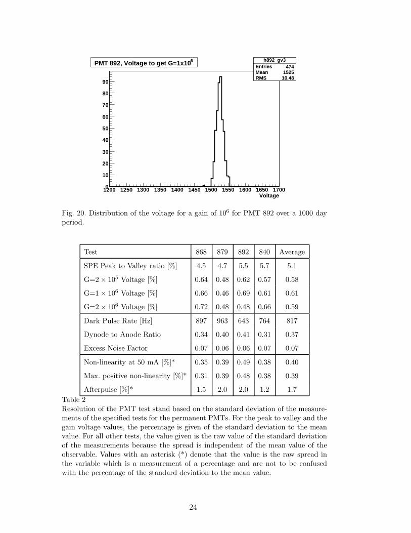
voltages. One PMT is taken as an example, PMT 892, to show the spread of450

the measurements over this same time period (see Fig. 20). For this PMT,451

the standard deviation is 10.5 V with a mean of 1525 ± 0.5 V. Fixing the452

voltage to the mean value, the standard deviation of the voltage corresponds453

to a standard deviation of less than 4% on the gain. Repeating this process454

for all the tests, the resolution of the system is determined for each test and455

is reported in Table 2.456

For an example of the monitoring capabilities of the four permanent PMTs,457

two examples are given. The first is shown in Fig. 21. In this figure, the dark458

pulse rate at 1/4 pe threshold is shown versus time, for 1000 days. For PMT459

879, there is a period of a steady decrease in the dark pulse rate, followed460

by a period of stability. This behavior is demonstrated solely by this PMT,461

therefore it is not necessary to make any corrections to the PMT test results.462

In the second example, however, in the non-linearity measurements there was463

a drift detected in the system starting around day 300 and recovering from464

day 500 to 600, see Fig. 22. Since all 4 PMTs experienced the same change465

in behavior (with PMT 879 experiencing an abrupt shift independently), the466

drift can be attributed to something that is happening in the test system itself467

and the results for the tested PMTs can be corrected for this behavior. The468

cause of this drift is unknown, but it can be monitored and the results can be469

adjusted accordingly.470

23

h892_gv3Entries 474Mean 1525RMS 10.48

Voltage1200 1250 1300 1350 1400 1450 1500 1550 1600 1650 17000

10

20

30

40

50

60

70

80

90

h892_gv3Entries 474Mean 1525RMS 10.48

6PMT 892, Voltage to get G=1x10

Fig. 20. Distribution of the voltage for a gain of 106 for PMT 892 over a 1000 dayperiod.

Test 868 879 892 840 Average

SPE Peak to Valley ratio [%] 4.5 4.7 5.5 5.7 5.1

G=2 × 105 Voltage [%] 0.64 0.48 0.62 0.57 0.58

G=1 × 106 Voltage [%] 0.66 0.46 0.69 0.61 0.61

G=2 × 106 Voltage [%] 0.72 0.48 0.48 0.66 0.59

Dark Pulse Rate [Hz] 897 963 643 764 817

Dynode to Anode Ratio 0.34 0.40 0.41 0.31 0.37

Excess Noise Factor 0.07 0.06 0.06 0.07 0.07

Non-linearity at 50 mA [%]* 0.35 0.39 0.49 0.38 0.40

Max. positive non-linearity [%]* 0.31 0.39 0.48 0.38 0.39

Afterpulse [%]* 1.5 2.0 2.0 1.2 1.7

Table 2Resolution of the PMT test stand based on the standard deviation of the measure-ments of the specified tests for the permanent PMTs. For the peak to valley and thegain voltage values, the percentage is given of the standard deviation to the meanvalue. For all other tests, the value given is the raw value of the standard deviationof the measurements because the spread is independent of the mean value of theobservable. Values with an asterisk (*) denote that the value is the raw spread inthe variable which is a measurement of a percentage and are not to be confusedwith the percentage of the standard deviation to the mean value.

24

Days100 200 300 400 500 600 700 800 900 1000

Dar

k P

uls

e R

ate

(kH

z)

0

1

2

3

4

5

6

7

8

9

10868

879

892

840

Dark Pulse Rate (0.25 pe Threshold)

Fig. 21. Dark pulse rate at 1/4 pe threshold for the four permanent PMTs. PMT879 experiences a steady decrease over the first 500 days.

Days100 200 300 400 500 600 700 800 900 1000

No

n-l

inea

rity

(%

)

-6

-4

-2

0

2

4

6868

879

892

840

Non-linearity at 50 mA

Fig. 22. Non-linearity at 50 mA for the four permanent PMTs. A system wide driftis noticed starting at day 300, peaking at day 500, and recovering at day 600.

To determine any systematic effect associated with location in the test stand,471

test results are also plotted as a function of position in the test stand, see472

Fig. 23. Each position in the test stand is in a fixed location, meaning the ori-473

entation with respect to the LEDs is constant. Each position is also associated474

with a fixed channel in the data acquisition electronics. In the plots in Fig. 23,475

each data point for the given location in the test stand has anywhere from 200476

to 350 PMTs to compute the average. In the bottom plot, it is shown that477

the mean dark pulse rate does not depend on the location in the test stand,478

25

Location2 4 6 8 10 12 14 16

Dar

k P

uls

e R

ate

[kH

z]

0

0.5

1

1.5

2

2.5

3

3.5

4

4.5

5

Dark Pulse Rate

Location2 4 6 8 10 12 14 16

No

n-l

inea

rity

[%

]

0

1

2

3

4

5

6

Maximum Positive Non-linearity

Fig. 23. Plots as a function of position in the test stand. In each, the red dashed lineis the mean value of that parameter for all tested PMTs Top: Maximum positivenon-linearity. Bottom: Dark pulse rate.

whereas non-linearity measurements (top plot) vary with the location in the479

test stand by around 1%. Any systematic effect due to the location in the test480

stand can be corrected in the final results.481

4 PMT Testing Conclusions482

The PMTs being used in the surface detector array for the Pierre Auger Ob-483

servatory are being thoroughly tested. For all the PMTs used in the surface484

26

detector, their characteristics and behavior are quantified in the PMT test485

system. These results are catalogued in a database for use in the analysis and486

monitoring of the surface detector. The tests run on the PMTs ensure uni-487

formity and quality in the performance of the surface detector and provide488

valuable feedback to the company producing them.489

The test system is capable of testing multiple PMTs in a single test run and is490

fully automated. This is necessary to be able to test all of the PMTs used in491

the surface detector of the Auger Observatory. Also, built into the test system492

is a monitoring system in the form of four permanent PMTs. These permanent493

PMTs provide valuable information to detect any anomalous behavior in the494

test system and also to understand the resolution of the tests run. The test495

results indicate that the PMTs used in the surface detector are well behaved496

and are quality photodetectors.497

References498

[1] J. Abraham et al., P. Auger Collaboration, Nucl. Instrum. Meth. A 523, 50499

(2004).500

[2] Pierre Auger Collaboration, Proc. 29th Intern. Cosmic Ray Conf., Pune, 7, 369501

(2005).502

[3] B. Genolini et al., Nucl. Instrum. Meth. A 504, 240 (2003).503

[4] A. Tripathi et al., Nucl. Instrum. Meth. A 497, 331 (2003).504

[5] X. Bertou et al., P. Auger Collaboration, Nucl. Instrum. Meth. A 568, 839505

(2006).506

[6] R.W. Engstrom, RCA Photomultiplier Handbook (PMT-62). Lancaster, PA:507

RCA Electro Optics and Devices (1980).508

[7] Pierre Auger Collaboration, Pierre Auger Project Design Report, second edition,509

November 1996. Revised March 14, 1997.510

[8] M.C. Teich, K. Matsuo, B.E.A. Saleh, IEEE Journal of Quantum Electronics511

22, 1184 (1986).512

27

Testing of Photomultiplier Tubes for Use in the Surface ... · Testing of Photomultiplier Tubes for...

Documents

Transcript of Testing of Photomultiplier Tubes for Use in the Surface ... · Testing of Photomultiplier Tubes for...