Testing normality of data on a multivariate grid

Journal of Multivariate Analysis 179 (2020) 104640

Contents lists available at ScienceDirect

Journal ofMultivariate Analysis

journal homepage: www.elsevier.com/locate/jmva

Testing normality of data on amultivariate gridLajos Horváth a,1, Piotr Kokoszka b,∗,1, Shixuan Wang c,1

a Department of Mathematics, University of Utah, Salt Lake City, UT 84112–0090, United Statesb Department of Statistics, Colorado State University, Fort Collins, CO 80523–1877, United Statesc Department of Economics, University of Reading, Reading, RG6 6AA, United Kingdom

a r t i c l e i n f o

Article history:Received 23 October 2019Received in revised form 14 May 2020Accepted 15 May 2020Available online 28 May 2020

AMS 2010 subject classifications:primary 62H11secondary 62F15

Keywords:Gaussian processLattice dataSignificance testSpatial statistics

a b s t r a c t

We propose a significance test to determine if data on a regular d-dimensional gridcan be assumed to be a realization of Gaussian process. By accounting for the spatialdependence of the observations, we derive statistics analogous to sample skewnessand kurtosis. We show that the sum of squares of these two statistics converges toa chi-square distribution with two degrees of freedom. This leads to a readily applicabletest. We examine two variants of the test, which are specified by two ways the spatialdependence is estimated. We provide a careful theoretical analysis, which justifies thevalidity of the test for a broad class of stationary random fields. A simulation studycompares several implementations. While some implementations perform slightly betterthan others, all of them exhibit very good size control and high power, even in relativelysmall samples. An application to a comprehensive data set of sea surface temperaturesfurther illustrates the usefulness of the test.

© 2020 Elsevier Inc. All rights reserved.

1. Introduction

Nearly all modern spatial statistics applications involve Gaussian processes. While for most large sample results itis not necessary to assume Gaussianity, it is often assumed to improve finite-sample inference and effectively applyBayesian methods. The same goes for nearly all applications involving conditional and simultaneous autoregressive modelsin discrete space, see the monographs of Cressie [7], Stein [39], Schabenberger and Gotway [34], Cressie and Wikle [8]and Banerjee et al. [5]. A survey of Gaussian modeling in spatial statistics is given by Gelfand and Schliep [14], part IIIof Gelfand et al. [13] specifically focuses on methods for discrete spatial data which rely on the Gaussian assumption, andthen those that do not. Recent research has focused on applying spatial statistics methods based on the assumption ofGaussianity to large data sets and advancing computational approaches, including parallel and distributed computing, see,e.g., Nychka et al. [26], Paciorek et al. [27], Katzfuss [20] and Guhaniyogi and Banerjee [15]. Methodology and theory forspatial Gaussian models continue to be developed, the references are very numerous. We note the recent work of Stroudet al. [41], which is concerned with missing values, and of Chang et al. [6] who study signal identification within themodel involving a Gaussian field on a grid.

Despite the prevalence of the assumption of Gaussianity, there appears to exist no significance tests that could be usedto assess if it is reasonable to assume that a given spatial data set can be treated as a realization of a Gaussian randomfield. This is a difficult problem because normality tests, and even exploratory tools like QQ-plots or histograms, require

∗ Corresponding author.E-mail address: [email protected] (P. Kokoszka).

1 All authors contributed equally to this work.

https://doi.org/10.1016/j.jmva.2020.1046400047-259X/© 2020 Elsevier Inc. All rights reserved.

https://doi.org/10.1016/j.jmva.2020.104640

http://www.elsevier.com/locate/jmva

http://www.elsevier.com/locate/jmva

http://crossmark.crossref.org/dialog/?doi=10.1016/j.jmva.2020.104640&domain=pdf

mailto:[email protected]


2 L. Horváth, P. Kokoszka and S. Wang / Journal of Multivariate Analysis 179 (2020) 104640

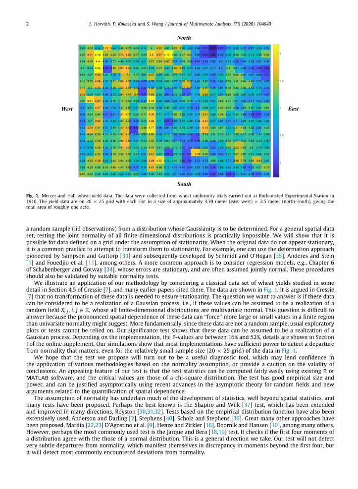
Fig. 1. Mercer and Hall wheat-yield data. The data were collected from wheat uniformity trials carried out at Rothamsted Experimental Station in1910. The yield data are on 20 × 25 grid with each slot in a size of approximately 3.30 meter (east–west) × 2.5 meter (north–south), giving thetotal area of roughly one acre.

a random sample (iid observations) from a distribution whose Gaussianity is to be determined. For a general spatial dataset, testing the joint normality of all finite-dimensional distributions is practically impossible. We will show that it ispossible for data defined on a grid under the assumption of stationarity. When the original data do not appear stationary,it is a common practice to attempt to transform them to stationarity. For example, one can use the deformation approachpioneered by Sampson and Guttorp [33] and subsequently developed by Schmidt and O’Hogan [35], Anderes and Stein[1] and Fouedjio et al. [11], among others. A more common approach is to consider regression models, e.g., Chapter 6of Schabenberger and Gotway [34], whose errors are stationary, and are often assumed jointly normal. These proceduresshould also be validated by suitable normality tests.

We illustrate an application of our methodology by considering a classical data set of wheat yields studied in somedetail in Section 4.5 of Cressie [7], and many earlier papers cited there. The data are shown in Fig. 1. It is argued in Cressie[7] that no transformation of these data is needed to ensure stationarity. The question we want to answer is if these datacan be considered to be a realization of a Gaussian process, i.e., if these values can be assumed to be a realization of arandom field Xi,j, i, j ∈ Z, whose all finite-dimensional distributions are multivariate normal. This question is difficult toanswer because the pronounced spatial dependence of these data can ‘‘force’’ more large or small values in a finite regionthan univariate normality might suggest. More fundamentally, since these data are not a random sample, usual exploratoryplots or tests cannot be relied on. Our significance test shows that these data can be assumed to be a realization of aGaussian process. Depending on the implementation, the P-values are between 16% and 52%, details are shown in SectionI of the online supplement. Our simulations show that most implementations have sufficient power to detect a departurefrom normality that matters, even for the relatively small sample size (20 × 25 grid) of the data in Fig. 1.

We hope that the test we propose will turn out to be a useful diagnostic tool, which may lend confidence inthe application of various methodologies based on the normality assumption, or provide a caution on the validity ofconclusions. An appealing feature of our test is that the test statistics can be computed fairly easily using existing R orMATLAB software, and the critical values are those of a chi-square distribution. The test has good empirical size andpower, and can be justified asymptotically using recent advances in the asymptotic theory for random fields and newarguments related to the quantification of spatial dependence.

The assumption of normality has underlain much of the development of statistics, well beyond spatial statistics, andmany tests have been proposed. Perhaps the best known is the Shapiro and Wilk [37] test, which has been extendedand improved in many directions, Royston [30,31,32]. Tests based on the empirical distribution function have also beenextensively used, Anderson and Darling [2], Stephens [40], Scholz and Stephens [36]. Great many other approaches havebeen proposed, Mardia [22,23] D’Agostino et al. [9], Henze and Zirkler [16], Doornik and Hansen [10], among many others.However, perhaps the most commonly used test is the Jarque and Bera [18,19] test. It checks if the first four moments ofa distribution agree with the those of a normal distribution. This is a general direction we take. Our test will not detectvery subtle departures from normality, which manifest themselves in discrepancy in moments beyond the first four, butit will detect most commonly encountered deviations from normality.

L. Horváth, P. Kokoszka and S. Wang / Journal of Multivariate Analysis 179 (2020) 104640 3

The paper is organized as follows. In Section 2 we develop the test. Its finite sample performance is evaluatedin Section 3 by means of a simulation study and an application to a climate data set. There are many possibleimplementations of our general paradigm, which must be evaluated and compared. The proofs of the mathematical resultsof Section 2, needed to derive and justify the test, are presented in Section II of an online supplement, which also containsadditional details of the test procedure and additional tables, which support our conclusions and recommendations.

2. Testing procedure and its large sample justification

We derive and formulate the testing procedure in Section 2.1, where we also specify the most important assumptionsfor its validity. A fundamental ingredient of our approach is the quantification and estimation of spatial dependence, thisis treated in Section 2.2. Asymptotic theory underlying both Sections 2.1 and 2.2 is developed in Section 2.3.

2.1. Assumptions and test derivation

Let Zd denote the set of d–dimensional vectors with integer coordinates. We assume that the observations Xi followthe model

Xi = µ + ei, i ∈ Zd,

where {ei} is a strictly stationary, zero mean spatial process. The mean µ is unknown.We want to test

H0 : the Xi are jointly normal,

against the alternative that H0 does not hold. The test is based on observations Xi, i ∈ Γn ⊂ Zd. The domain Γn is indexedby positive integers n, which are not sample sizes, but sample indexes in increasing domain asymptotics. The sample sizeis denoted by nΓ , the cardinality of the set Γn, nΓ = |Γn|. If d = 2, and Γn = ΓN,M := {(i, j), 1 ≤ i ≤ N, 1 ≤ j ≤ M}, thennΓ = NM . Let ∂Γn denote the boundary of Γn and |∂Γn| its cardinality. We assume that, as n → ∞,

|∂Γn|

nΓ

→ 0. (1)

Condition (1) states that asymptotically there should be many more points in the interior of the domain than at itsboundary. If d = 2, and Γn = ΓN,M , defined above, then (1) holds if and only of min(N,M) → ∞.

We assume that under the null hypothesis {ei} is a Gaussian spatial linear process, i.e., it satisfies the followingassumption.

Assumption 1. The ei are spatial moving averages,

ei =

∑s∈Zd

asεi−s, i ∈ Zd, (2)

with independent, standard normal innovations εi, and the coefficients as satisfying∑s∈Zd

|as| < ∞. (3)

Assumption 1 implies that the field {Xi} is strictly stationary and Gaussian, with spatial dependence quantified byconditions (2) and (3). Linearity in (2) is needed to ensure normality of the observations. The summability condition in(3) cannot be relaxed because the required CLT would not hold with standard rate, see Lahiri and Robinson [21]. UnderAssumption 1, the random variables

zi =Xi − µ

σ, with σ 2

=

∑s∈Zd

a2s , (4)

are standard normal (but, in general, not independent). The zi must be approximated by random variables that can becomputed from the sample. For this purpose, define

S2n =1nΓ

∑i∈Γn

(Xi − Xn)2, Xn =1nΓ

∑i∈Γn

Xi.

Our tests statistics are based on the standardized observations

xi = xi,n =Xi − Xn

Sn, i ∈ Γn, (5)


which are sample counterparts of the standard normal zi defined above. Using the xi, we define the sample skewness andkurtosis by

Sn =1

n1/2Γ

∑i∈Γn

x3i and Kn =1

n1/2Γ

∑i∈Γn

(x4i − 3). (6)

As we will see in Section 2.3, the asymptotic variances of Sn and Kn are, respectively,

φ2S =

∑i∈Zd

E[(z30 − 3z0)(z3i − 3zi)

](7)

and

φ2K =

∑i∈Zd

E[(z40 − 6z20 + 3)(z4i − 6z2i + 3)

]. (8)

In particular,

φ2K =

∑i∈Zd

E[(z40 − 3)(z4i − 3)

].

This motivates the introduction of modified sample skewness and kurtosis defined by

S⋆n =

1

n1/2Γ

∑i∈Γn

(x3i − 3xi) and K⋆n =

1

n1/2Γ

∑i∈Γn

(x4i − 6x2i + 3).

Observe that S⋆n = Sn because

∑i∈Γn

xi = 0. The statistics S⋆n and K⋆

n also have asymptotic variances, respectively, φ2S

and φ2K, and are better matched to them in finite samples because φ2

S and φ2K are direct counterparts of spatial long-run

variances of the sequences{x3i − 3xi

}and

{x4i − 6x2i + 3

}.

Denoting by φS and φK consistent estimators of φS and φK, the test statistic is defined as

J⋆n =S⋆2n

φ2S

+K⋆2

n

φ2K

.

It is the sum of squares of normalized skewness and kurtosis. As will be stated in Section 2.3, J⋆n is asymptotically chi-squarewith two degrees of freedom. The test thus is:

Reject H0 at significance level α if J⋆n > χ22 (1 − α), where χ2

2 (1 − α) is the (1 − α)th quantile of the chi-square distributionwith two degrees of freedom.

Suitable estimators φ2S and φ2

K are derived in Section 2.2, see formulas (12) and (13).The key to understanding the need for the modified kurtosis is the fact that

φ2K =

∑i∈Zd

E[(z40 − 3)(z4i − 3)

].

The formula given above must be used instead, which is the long-run variance of the unobservable field{z4i − 6z2i + 3

}.

We replace the zi by the observable xi, which approximate them with an asymptotically negligible effect. In particular,Var[K⋆

n] = φ2K, so K⋆2

n divided by an estimator of the variance of K⋆n is a Wald statistic, which is asymptotically χ2

1 . (Thepopulation kurtosis is zero under the null hypothesis.) The same argument applies the skewness. We show that these twocomponents are asymptotically independent, so their sum is asymptotically χ2

2 .

2.2. Estimation of the spatial long run variances

It is useful to consider a more general setting. Suppose{yi, i ∈ Zd

}is a zero mean strictly stationary scalar random

field such that Ey20 < ∞, whose covariances are γ (j) = E[y0yj], j ∈ Zd. The objective is to estimate the long-run, orasymptotic, variance defined by

σ 2=

∑j∈Zd

γ (j) =

∑j∈Zd

E[y0yj]. (9)

We assume throughout that∑j∈Zd

|γ (j)| < ∞, (10)

so that σ 2 can be defined. We observe yj ∈ Γn, which is a rectangle whose all dimensions are increasing, as specified inthe following assumption.


Assumption 2. The spatial domain Γn is given by

Γn = {1, . . . , n1} × {1, . . . , n2} × · · · × {1, . . . , nd]

and n⋆:= min1≤i≤d ni → ∞.

The sample covariances are defined by

γ (j) = |Γn(j)|−1∑i∈Γn(j)

yiyi+j, where Γn(j) = {i ∈ Γn : i + j ∈ Γn} .

To provide explicit formulas, in the following we use the notation j = (j1, . . . , jd). In this setting, σ 2 is estimated by thekernel estimator

σ 2n =

d∑ℓ=1

∑|jℓ|≤nℓ

{d∏

ℓ=1

K(

jℓhℓ

)}γ (j1, . . . , jd), (11)

where K is a univariate kernel satisfying the following commonly used assumption.

Assumption 3. The kernel K is a continuous function on the interval [−1, 1] satisfying K (0) = 1. The bandwidths hℓ

satisfy h⋆:= max1≤ℓ≤d hℓ → ∞, as n → ∞.

In our context, we use estimator (11) computed from yi = x3i − 3xi and yi = x4i − 6xi + 3. These yi do not form astrictly stationary random field. Due to the random normalization in (5), they form a structure which could be called aspatial triangular array. However, the zi defined by (4) do form a strictly stationary random field, so it must be shownthat replacing the xi by the zi introduces an asymptotically negligible effect into the estimation of φ2

S and φ2K. This will

be established in the proof of Theorem 2. We first introduce the required notation. Set

ySi = x3i − 3xi, yKi = x4i − 6xi + 3

and

yS =1nΓ

∑i∈Γn

ySi , yK =1nΓ

∑i∈Γn

yKi .

Next, we define the sample covariances

γS(j) = |Γn(j)|−1∑i∈Γn(j)

(ySi − yS

) (ySi+j − yS

),

γK(j) = |Γn(j)|−1∑i∈Γn(j)

(yKi − yK

) (yKi+j − yK

).

Using notation∑j∈J(h)

wh(j)g(j) =

d∑ℓ=1

∑|jℓ|≤nℓ

{d∏

ℓ=1

K(

jℓhℓ

)}g(j1, . . . , jd),

which applies to any function g on Zd, we define the kernel estimators

φ2S,kern =

∑j∈J(h)

wh(j)γS(j), φ2K,kern =

∑j∈J(h)

wh(j)γK(j). (12)

The idea behind the kernel estimators is as follows. Focus on φ2K,kern and consult formula (8). We replace the model

autocovariances E[(z40 − 6z20 + 3)(z4j − 6z2j + 3)

]by the sample autocovariances γK(j). The latter are variable if the set

Γn(j) is small, i.e., if j is ‘‘spatially large". For this reason, we put smaller weights on them. This idea has been commonlyused in time series analysis.

Another class of estimators can be derived as follows. Set ρi = E[z0zi]. Tedious calculations, using the values of themoments of the standard normal distributions, show that

φ2S = 6

∑i∈Zd

ρ3i and φ2

K = 24∑i∈Zd

ρ4i .

We estimate the ρi by the sample covariances of the xi, i.e., by (recall that x = 0)

γx(j) = |Γn(j)|−1∑i∈Γn(j)

xixi+j


and define the power estimators

φ2S,pow = 6

∑j∈J(h)

wh(j)γ 3x (j), φ2

K,pow = 24∑j∈J(h)

wh(j)γ 4x (j), (13)

i.e.,

φ2S,pow = 6

d∑ℓ=1

∑|jℓ|≤hℓ

{d∏

ℓ=1

K(

jℓnℓ

)}γ 3x (j1, . . . , jd),

φ2K,pow = 24

d∑ℓ=1

∑|jℓ|≤hℓ

{d∏

ℓ=1

K(

jℓnℓ

)}γ 4x (j1, . . . , jd).

The consistency of the above spatial long-run variance estimators is established in Section 2.3. More explicit formulasfor the commonly encountered case of a 2D rectangular domain are given in Section III of the Supplement.

2.3. Asymptotic theory

This section contains asymptotic results, which justify the application of the test for a large class of stationary fields.All proofs are given in Section II of the supplement. The first result establishes the asymptotic distribution of the sampleskewness Sn and kurtosis Kn, and their modified versions S⋆

n and K⋆n. Very little must be assumed about the shape of the

spatial domain Γn.

Theorem 1. Suppose condition (1) and Assumption 1 hold. Then the series (7) and (8) defining, respectively, φ2S and φ2

K areabsolutely convergent, and the vectors [Sn,Kn]

⊤ and [S⋆n,K

⋆n]

⊤ both converge to the bivariate normal distribution with meanzero and covariance matrix[

φ2S 00 φ2

K

].

Based on Theorem 1, we consider the test statistics

Jn =S2n

φ2S

+K2

n

φ2K

and J⋆n =S⋆2n

φ2S

+K⋆2

n

φ2K

.

The following corollary is an immediate consequence of Theorem 1.

Corollary 1. Suppose condition (1) and Assumption 1 hold, and

φ2S

P→ φ2

S and φ2K

P→ φ2

K. (14)

Then JnD

→ χ22 and J⋆n

D→ χ2

2 , where χ22 is a chi-square random variable with two degrees of freedom.

We now turn to the consistency of the estimators given by (12) and (13). For these results more restrictive assumptionson the spatial domain are required. Recall that n⋆

:= min1≤i≤d ni and h⋆= max1≤ℓ≤d hℓ.

Theorem 2. Suppose (1), Assumptions 1–3 hold, and h⋆= o(n⋆1/2). Then relations (14) hold for the estimators φ2

S,kern andφ2K,kern given by (12) and the estimators φ2

S,pow and φ2K,pow given by (13).

Estimation of the spatial long-run variance σ 2 given by (9) has been recently studied by Prause and Steland [29] whoestablished consistency assuming ϕ-mixing with a suitable rate. If the errors εj are normal, even for d = 1, the movingaverage (2) is ϕ-mixing if only finitely many coefficients as are not zero, see Ibragimov and Linnik [17] and Sidorov [38].For this reason, we use a different, more direct, approach to prove Theorem 2.

We now turn to the consistency of the test. We begin with an assumption which is essentially Assumption 1, butwithout assuming normality.

Assumption 4. The ei are moving averages (2) with independent and identically distributed random variables εi, satisfyingEεℓ = 0, Eε2

ℓ = 1, Eε8ℓ < ∞, and the coefficients as satisfying (3).

Under Assumption 4, we can establish limits in probability of n−1/2Γ S⋆

n and n−1/2Γ K⋆

n, as stated in Theorem 3. Notice thatunder H0 these limits are zero.

Theorem 3. If (1) and Assumption 4 hold, then

n−1/2Γ S⋆

nP

→ Ez30 and n−1/2Γ K⋆

nP

→ Ez40 − 3,

where z0 is defined by (4). The limit of n−1/2Γ Kn is the same as the limit of n−1/2

Γ K⋆n.


Next we establish bounds on magnitudes of the estimators of the long-run variances.

Theorem 4. Suppose (1) and Assumptions 3 and 4 hold, and h⋆= o(n⋆1/2). Then

φ2S,kern = OP (h⋆), φ2

K,kern = OP (h⋆)

and

φ2S,pow = OP (1), φ2

K,pow = OP (1).

Using Theorems 3 and 4, we can prove the consistency of the test.

Corollary 2. If the conditions of Theorem 4 are satisfied and if Ez30 = 0 and/or Ez40 = 3, then JnP

→ ∞ and J⋆nP

→ ∞.

3. Finite sample performance and application to temperature data

In Section 3.1, we explore the empirical size and power of several implementations of our test. In Section 3.2, we checkif the spatial fields of sea surface temperature anomalies can be assumed to be Gaussian, and provide further insights intothe behavior of the test.

3.1. A simulation study

In this section, we use Monte Carlo simulation to assess finite sample properties of the test derived in Section 2.1. Wefocus on the case of d = 2, most commonly encountered in applications. Explicit formulas in this case are given in SectionIII of the Supplement. We consider data generating processes (DGPs) defined by three different spatial models specifiedbelow, and by several grid sizes. We use 5000 independent replications, and record the count of rejections to calculateempirical size and power of the proposed test.

We generate realizations on a grid {1 ≤ i, j ≤ N} of the following spatial models:

Spatial IID: Xi,j = 2 +√2ξi,j.

Spatial Moving-average (MA): Xi,j = ξi,j + 0.5ξi,j−1.Spatial Autoregressive(AR): Xi,j = 0.5Xi−1,j−1 + ξi,j.

Under H0, ξi,j ∼ i.i.d. N (0, 1). We consider two error distributions under HA: the ξi,j are i.i.d. with either Student’st-distribution with ν degrees of freedom or with the skew-normal distribution. We set ν to values ranging from 5 to 20.If ν ≥ 30, the univariate t-distribution is visually almost indistinguishable from the standard normal distribution, andits quantiles are almost equal to the standard normal quantiles. Unlike the t-distribution, the skew-normal distribution,treated in Azzalini [4], has nonzero skewness. Further details and power tables are presented in Section IV of theSupplement.

Both the kernel and power estimators, defined in Section 2.2 (and Section III of the Supplement), need the specificationof the kernel and the smoothing bandwidth. Three kernel functions are compared.

The truncated kernel (TR): KTR (t) = I {|t| ⩽ 1}.The Bartlett kernel (BT): KBT (t) = (1 − |t|) I {|t| ⩽ 1}.The flat-top kernel (FT):

KFT (t) =

⎧⎨⎩1, 0 ⩽ t < 0.52 − |t| , 0.5 ⩽ t < 10, 1 ⩽ t.

The bandwidth h for these kernels is selected as

hTR = ⌊4(N/100)1/5⌋, hBT = ⌊4(N/100)2/9⌋, hFT = ⌊4(N/100)1/5⌋. (15)

The choice of the smoothing bandwidth has been well studied. For the truncated and Bartlett kernels, Newey andWest [25]compared the performance of different plug-in methods, while Andrews [3] proposed a data-driven bandwidth selectiontechnique. Politis [28] developed an adaptive bandwidth choice for the flat-top kernel. It turns out that these choiceswork well for our purpose. We thus follow Newey and West [25] to select the bandwidth for the truncated and Bartlettkernels. Our simulations showed that choosing the bandwidth of the flat-top kernel the same as for the truncated kernelproduces stable and satisfactory results.

Empirical size Table 1 reports the empirical sizes, the percentages of rejections under H0. As can be seen, the empiricalsizes are close to the theoretical levels, even for small grid size, such as N = 100. Comparing the results for the kernelestimator and the power estimator, it seems that there is no obvious pattern in the empirical sizes. The differences arising


Table 1The empirical sizes of 5000 independent simulations with significant levels of 10%, 5%, and 1% for the spatial normalitytests based on the kernel estimators φ2

S,kern, φ2K,kern and the power estimators φ2

S,pow, φ2K,pow for three DGPs of spatial

IID (Xi,j = 2+√2ξi,j), spatial moving-average (Xi,j = ξi,j +0.5ξi,j−1), spatial autoregressive(Xi,j = 0.5Xi−1,j−1 +ξi,j), where

ξi,j ∼ i.i.d. N (0, 1).

Grid size Kernel Kernel estimator Power estimator

10% 5% 1% 10% 5% 1%

Panel A: Spatial IID

N = 100Truncated 10.12% 4.92% 1.10% 10.52% 4.96% 1.16%Bartlett 9.52% 4.54% 1.08% 10.52% 4.96% 1.16%Flat-top 9.54% 4.84% 1.10% 10.52% 4.96% 1.16%



Panel B: Spatial moving average




Panel C: Spatial autoregressive




from the application of different kernels are small and do not exhibit any clear pattern either. We conclude that our testcontrols size very well, not matter which one of the six considered implementations is used.

Empirical power Tables 2 and 3 present the empirical power of the test by 5% significance level critical values with thespatial long run variance estimated, respectively, by the kernel estimator and the power estimator. As expected, the powerincreases with the grid size N . Comparing the results for the three DGPs, we find that the test has higher power underthe spatial IID than the two models with spatial dependence. This could be expected, as both the MA and AR modelslead to some averaging of the ξi,j, bringing the observations Xi,j a bit closer to normality. There is no apparent differencewhen using different kernels under the spatial IID, but the Bartlett kernel occasionally has marginally higher power underthe spatial MA and AR models. An important observation is that different results are produced by using the two spatiallong run variance estimators. When the power estimator is used, the power is monotonously decreasing as the degrees offreedom ν of the ξi,j grow. However, this pattern does not occur when the kernel estimator is employed. To be specific forthe kernel estimator, the expected power behavior is observed for ν > 8, but not for ν ⩽ 8. A reasonable explanation isthat we use the 8th moment of the Student’s t-distribution when estimating φ2

K. However, the kth moment of a Student’st random variable is well-defined only for k < ν. For the power estimator, we only use the 4th moment of observationsin the spatial models generated by the Student’s t random variable. Comparing Tables 2 and 3, we can conclude that thepower estimator has better power properties than the kernel estimator. Additionally, the power estimator is more broadlyapplicable as it requires fewer moments of the data. We note that the kernel estimator requires the existence of first eightmoments of the distribution, but we are still interested in the impact on power of the kernel estimator if some of the firsteight moments do not exist. Thus, we also report the power of the kernel estimator for ν = 8, 5 in Table 2. The empiricalpower when the skew-normal distribution is employed, has similar behavior, except that we do not see nonmonotonic


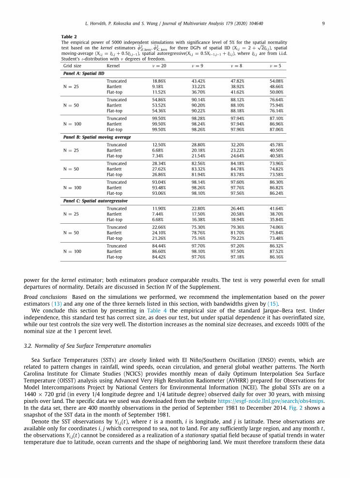
Table 2The empirical power of 5000 independent simulations with significance level of 5% for the spatial normalitytest based on the kernel estimators φ2

S,kern, φ2K,kern for three DGPs of spatial IID (Xi,j = 2 +

√2ξi,j), spatial

moving-average (Xi,j = ξi,j + 0.5ξi,j−1), spatial autoregressive(Xi,j = 0.5Xi−1,j−1 + ξi,j), where ξi,j are from i.i.d.Student’s t-distribution with ν degrees of freedom.Grid size Kernel ν = 20 ν = 9 ν = 8 ν = 5


N = 25Truncated 18.86% 43.42% 47.82% 54.08%Bartlett 9.18% 33.22% 38.92% 48.66%Flat-top 11.52% 36.70% 41.62% 50.00%











power for the kernel estimator; both estimators produce comparable results. The test is very powerful even for smalldepartures of normality. Details are discussed in Section IV of the Supplement.

Broad conclusions Based on the simulations we performed, we recommend the implementation based on the powerestimators (13) and any one of the three kernels listed in this section, with bandwidths given by (15).

We conclude this section by presenting in Table 4 the empirical size of the standard Jarque–Bera test. Underindependence, this standard test has correct size, as does our test, but under spatial dependence it has overinflated size,while our test controls the size very well. The distortion increases as the nominal size decreases, and exceeds 100% of thenominal size at the 1 percent level.

3.2. Normality of Sea Surface Temperature anomalies

Sea Surface Temperatures (SSTs) are closely linked with EI Niño/Southern Oscillation (ENSO) events, which arerelated to pattern changes in rainfall, wind speeds, ocean circulation, and general global weather patterns. The NorthCarolina Institute for Climate Studies (NCICS) provides monthly mean of daily Optimum Interpolation Sea SurfaceTemperature (OISST) analysis using Advanced Very High Resolution Radiometer (AVHRR) prepared for Observations forModel Intercomparisons Project by National Centers for Environmental Information (NCEI). The global SSTs are on a1440 × 720 grid (in every 1/4 longitude degree and 1/4 latitude degree) observed daily for over 30 years, with missingpixels over land. The specific data we used was downloaded from the website https://esgf-node.llnl.gov/search/obs4mips.In the data set, there are 400 monthly observations in the period of September 1981 to December 2014. Fig. 2 shows asnapshot of the SST data in the month of September 1981.

Denote the SST observations by Yi,j(t), where t is a month, i is longitude, and j is latitude. These observations areavailable only for coordinates i, j which correspond to sea, not to land. For any sufficiently large region, and any month t ,the observations Yi,j(t) cannot be considered as a realization of a stationary spatial field because of spatial trends in watertemperature due to latitude, ocean currents and the shape of neighboring land. We must therefore transform these data

https://esgf-node.llnl.gov/search/obs4mips


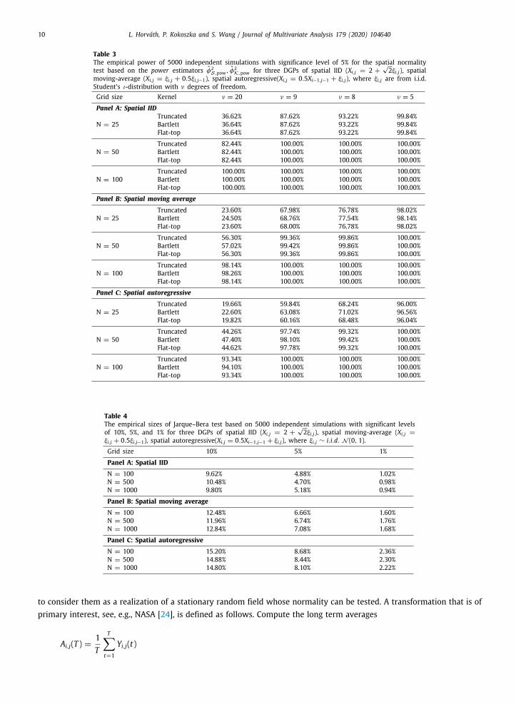
Table 3The empirical power of 5000 independent simulations with significance level of 5% for the spatial normalitytest based on the power estimators φ2

S,pow, φ2K,pow for three DGPs of spatial IID (Xi,j = 2 +

√2ξi,j), spatial

moving-average (Xi,j = ξi,j + 0.5ξi,j−1), spatial autoregressive(Xi,j = 0.5Xi−1,j−1 + ξi,j), where ξi,j are from i.i.d.Student’s t-distribution with ν degrees of freedom.Grid size Kernel ν = 20 ν = 9 ν = 8 ν = 5













Table 4The empirical sizes of Jarque–Bera test based on 5000 independent simulations with significant levelsof 10%, 5%, and 1% for three DGPs of spatial IID (Xi,j = 2 +

√2ξi,j), spatial moving-average (Xi,j =

ξi,j + 0.5ξi,j−1), spatial autoregressive(Xi,j = 0.5Xi−1,j−1 + ξi,j), where ξi,j ∼ i.i.d. N (0, 1).

Grid size 10% 5% 1%

Panel A: Spatial IIDN = 100 9.62% 4.88% 1.02%N = 500 10.48% 4.70% 0.98%N = 1000 9.80% 5.18% 0.94%

Panel B: Spatial moving averageN = 100 12.48% 6.66% 1.60%N = 500 11.96% 6.74% 1.76%N = 1000 12.84% 7.08% 1.68%

Panel C: Spatial autoregressiveN = 100 15.20% 8.68% 2.36%N = 500 14.88% 8.44% 2.30%N = 1000 14.80% 8.10% 2.22%

to consider them as a realization of a stationary random field whose normality can be tested. A transformation that is ofprimary interest, see, e.g., NASA [24], is defined as follows. Compute the long term averages

Ai,j(T ) =1T

T∑t=1

Yi,j(t)


Fig. 2. SST data snapshot in September 1981 and the four selected regions. The global SST data is on a 1440 × 720 grid (in every 1/4 longitudedegree and 1/4 latitude degree), with missing pixels over land. Region 1 (longitude 60◦ to 90◦ , latitude −30◦ to 0◦) lies in Indian Ocean and in thesouthern hemisphere. Region 2 (longitude 170◦ to 200◦ , latitude −15◦ to 15◦) is located in the Pacific Ocean and it is symmetric by the equator.Region 3 (longitude 210◦ to 240◦ , latitude −50◦ to −20◦) is in the Pacific Ocean but it is in the southern hemisphere, away from the equator. Region4 (longitude 305◦ to 335◦ , latitude 10◦ to 40◦) is in the Northern Atlantic. Each selected region is on a 120 × 120 grid, containing 30◦ of longitudeand 30◦ of latitude.

Table 5P-values of the spatial normality test for Di,j(t) in July. Bold numbers indicate rejections at the 5% significance level.

Date Kernel estimator Power estimator

Region 1 Region 2 Region 3 Region 4 Region 1 Region 2 Region 3 Region 4

Jul-1982 3.3% 0.0% 36.7% 0.0% 9.0% 0.0% 34.5% 0.0%Jul-1983 47.4% 0.0% 0.0% 0.0% 46.4% 1.8% 1.6% 0.0%Jul-1984 0.0% 0.1% 0.0% 0.0% 0.0% 1.4% 2.5% 0.0%Jul-1985 0.0% 0.0% 0.1% 0.0% 0.4% 0.0% 0.0% 0.4%Jul-1986 4.7% 0.0% 84.8% 0.0% 5.4% 0.2% 85.8% 0.0%Jul-1987 27.0% 1.4% 71.4% 0.0% 45.5% 11.8% 73.5% 0.0%Jul-1988 11.9% 0.0% 1.5% 3.6% 8.0% 0.0% 3.2% 16.0%Jul-1989 0.5% 0.0% 0.3% 0.0% 0.3% 0.0% 8.0% 0.0%Jul-1990 0.1% 0.0% 0.0% 0.0% 0.0% 0.0% 1.5% 0.0%Jul-1991 0.3% 0.0% 0.0% 0.0% 6.6% 0.0% 0.0% 0.0%Jul-1992 0.0% 50.1% 0.0% 0.0% 0.0% 57.6% 0.1% 0.0%Jul-1993 11.5% 0.0% 0.0% 0.0% 0.0% 0.4% 0.0% 0.0%Jul-1994 4.1% 0.0% 0.1% 0.0% 20.3% 0.0% 1.4% 0.0%Jul-1995 0.0% 31.6% 1.9% 0.0% 0.1% 58.7% 1.8% 0.0%Jul-1996 11.0% 0.0% 0.0% 0.0% 25.4% 0.0% 1.0% 0.1%Jul-1997 0.8% 0.0% 74.2% 0.0% 10.2% 0.3% 52.5% 0.0%Jul-1998 1.0% 0.0% 1.9% 15.6% 5.3% 0.0% 4.0% 33.7%Jul-1999 0.1% 0.0% 0.0% 10.4% 3.3% 0.0% 0.0% 18.6%Jul-2000 0.5% 0.0% 0.0% 0.0% 3.4% 0.0% 0.0% 0.0%Jul-2001 0.0% 0.0% 0.0% 0.7% 0.0% 0.0% 0.1% 12.4%Jul-2002 7.8% 0.0% 0.0% 0.0% 34.0% 0.0% 0.0% 0.0%Jul-2003 0.0% 0.0% 57.8% 0.0% 0.0% 0.0% 49.6% 0.2%Jul-2004 2.9% 18.5% 51.9% 0.0% 2.8% 26.5% 66.6% 0.1%Jul-2005 1.5% 5.2% 0.0% 0.0% 0.0% 2.1% 0.1% 0.3%Jul-2006 0.2% 23.8% 54.0% 0.0% 0.0% 40.3% 57.0% 0.0%Jul-2007 0.0% 0.0% 8.9% 0.0% 0.0% 0.0% 0.9% 0.3%Jul-2008 37.0% 0.0% 0.1% 0.0% 41.9% 0.0% 0.0% 0.0%Jul-2009 34.3% 0.3% 48.9% 0.0% 45.6% 9.5% 56.8% 0.0%Jul-2010 4.1% 9.7% 0.0% 0.0% 13.2% 21.5% 0.3% 0.0%Jul-2011 0.0% 0.0% 0.6% 0.0% 0.3% 0.0% 13.8% 0.0%Jul-2012 0.0% 0.0% 0.0% 0.1% 0.3% 0.0% 1.0% 2.5%Jul-2013 0.0% 0.0% 12.1% 0.6% 0.1% 0.1% 4.0% 0.1%Jul-2014 0.2% 0.0% 53.7% 0.8% 0.3% 0.0% 49.4% 2.0%

where T is number of the same calendar months in the sample period. For example, if t corresponds to July, and we haveT = 33 Julys in the sample period. The monthly anomalies are defined as

Di,j(t) = Yi,j(t) − Ai,j(T ).


Table 6P-values of the spatial normality test for Ui,j(t) in July. Bold numbers indicate rejections at the 5% significance level.

Date Kernel estimator Power estimator

Region 1 Region 2 Region 3 Region 4 Region 1 Region 2 Region 3 Region 4

Jul-1982 11.3% 0.0% 0.0% 0.0% 40.3% 0.0% 0.0% 0.0%Jul-1983 1.3% 0.0% 0.1% 0.0% 13.1% 0.0% 0.7% 0.0%Jul-1984 0.0% 6.8% 0.0% 0.0% 0.2% 29.3% 0.1% 0.0%Jul-1985 0.0% 0.0% 1.2% 0.0% 0.1% 1.0% 3.2% 1.2%Jul-1986 0.4% 0.0% 0.3% 0.0% 0.1% 0.0% 6.3% 0.0%Jul-1987 3.9% 0.0% 77.7% 0.0% 5.9% 0.6% 83.5% 0.0%Jul-1988 56.3% 0.0% 5.8% 0.0% 70.9% 0.1% 15.8% 0.0%Jul-1989 19.4% 0.0% 0.0% 0.0% 40.4% 0.0% 0.1% 0.0%Jul-1990 70.5% 0.1% 1.6% 0.1% 82.5% 0.3% 7.7% 0.4%Jul-1991 0.0% 0.0% 0.0% 0.0% 0.3% 1.9% 0.0% 0.0%Jul-1992 8.0% 0.1% 0.0% 0.0% 12.1% 0.1% 0.0% 0.3%Jul-1993 38.6% 0.0% 0.0% 0.2% 63.6% 0.0% 1.7% 2.5%Jul-1994 17.9% 0.0% 0.0% 0.0% 43.1% 0.0% 1.5% 0.0%Jul-1995 0.3% 43.0% 5.8% 0.0% 6.6% 47.3% 9.7% 0.0%Jul-1996 0.0% 1.4% 1.4% 0.0% 2.3% 14.4% 3.4% 0.1%Jul-1997 0.0% 0.0% 59.1% 0.0% 0.3% 0.0% 66.8% 0.0%Jul-1998 0.2% 0.1% 0.1% 0.0% 6.9% 4.4% 1.9% 0.0%Jul-1999 0.7% 0.0% 0.0% 3.2% 12.0% 0.0% 0.0% 7.6%Jul-2000 0.0% 0.0% 0.0% 0.0% 1.4% 0.0% 0.0% 0.0%Jul-2001 0.0% 0.0% 0.0% 0.0% 0.0% 0.1% 0.0% 0.3%Jul-2002 1.2% 0.0% 0.0% 0.0% 16.1% 1.1% 0.0% 0.0%Jul-2003 0.1% 0.0% 53.9% 0.0% 0.3% 0.0% 48.8% 2.6%Jul-2004 11.0% 0.0% 0.0% 0.0% 21.1% 0.0% 0.8% 0.1%Jul-2005 96.4% 45.2% 0.0% 0.0% 97.4% 48.6% 0.5% 0.0%Jul-2006 3.1% 46.0% 0.0% 0.1% 2.4% 60.6% 2.5% 0.8%Jul-2007 10.4% 0.0% 0.0% 0.0% 10.1% 0.0% 0.0% 0.1%Jul-2008 0.4% 0.0% 13.6% 4.7% 5.4% 0.0% 0.3% 6.7%Jul-2009 35.2% 0.4% 6.1% 0.0% 59.5% 8.8% 18.0% 0.0%Jul-2010 0.1% 0.0% 30.9% 0.0% 4.1% 0.0% 54.4% 0.0%Jul-2011 3.9% 0.0% 0.0% 0.0% 19.8% 0.0% 0.0% 0.0%Jul-2012 0.0% 0.0% 0.0% 0.0% 0.2% 0.0% 0.6% 1.2%Jul-2013 13.3% 0.0% 34.2% 76.3% 25.5% 0.0% 44.9% 81.3%Jul-2014 9.1% 0.0% 0.0% 0.0% 28.2% 0.0% 1.5% 1.2%

They are deviations in a given year from what is typical for a given month at location (i, j). As quantified by French et al.[12], among others, surface temperatures exhibit complex spatial trends in their variability. These are more pronouncedover continents (temperatures over coastal regions are less variable that those in the interior), but one can expect a similar,though smaller, effect over bodies of water. We therefore also consider standardized anomalies defined by

Ui,j(t) =Yi,j(t) − Ai,j(T )

SDi,j(T ),

where

SD2i,j(T ) =

1T

T∑t=1

(Yi,j(t) − Ai,j(T ))2.

As spatial domains, we selected four squared ocean regions with different characteristics. Region 1 (longitude 60◦ to90◦, latitude -30◦ to 0◦) lies in Indian Ocean and in the southern hemisphere. Region 2 (longitude 170◦ to 200◦, latitude−15◦ to 15◦) is located in the Pacific Ocean and it is symmetric by the equator. Region 3 (longitude 210◦ to 240◦, latitude−50◦ to −20◦) is also in the Pacific Ocean but it is in the southern hemisphere, away from the equator. The last region,Region 4 (longitude 305◦ to 335◦, latitude 10◦ to 40◦) is in the Northern Atlantic. The data over these regions are on a120 × 120 grid, due to the fact that they all contain an area extending 30◦ of longitude and 30◦ of latitude. The fourselected regions are highlighted in Fig. 2.

Conclusions from the application of the normality test We applied the implementations with both the kernel and the powerestimator in order to see if the differences observed in Section 3.1 manifest themselves for the temperature data. It turnsout that the kernel and the power estimators produce consistent results in the most cases, but not in all cases. We onlyreports results for the flat-top kernel as other kernels produce similar results.

The P-values for July in all years of the sample period for Di,j(t) and Ui,j(t) are shown in Tables 5 and 6, respectively. TheP-values for January, April, and October are provided in the Supplement. The most general observation is that normality ofthese spatial data cannot be assumed without further checks, so spatial statistics methods which rely on the assumptionof Gaussianity must be used with caution. It might be best to use methods which do not assume Gaussianity. Comparing


the results for the two versions of monthly anomalies, Di,j(t) and Ui,j(t), they generally lead to the same conclusion, butUi,j(t) tends to produce more acceptances of normality, indicated by the P-values greater than 5%. This effect is howevernot very large. By looking at the results in different four regions, we see that Region 1, which is in the Indian Ocean and inthe southern hemisphere, is the one with the highest number of normality in the July monthly anomalies for all years. Inparticular, the test on the second version of monthly anomalies, Ui,j(t), using the power estimator for the long run variancesuggests the normality in 21 out of 33 years. On the opposite side, Region 4, which is located in the Atlantic Ocean and inthe northern hemisphere, has the lowest number of acceptances of normality of the July monthly anomalies. Specifically,Ui,j(t) with the power estimator only suggests the normality in 3 out of 33 years. These conclusions also hold for othermonths.

Acknowledgments

We are grateful to the Editor-in-Chief, Associate Editor, and reviewers for their valuable comments and suggestions,which have led to an improved version of this paper. We would also like to thank Professor Anil K. Bera for his helpfuldiscussions at the 4th Workshop on ‘‘Goodness-of-fit, Change-point and Related Problems’’ (Trento, Italy, 2019). Thisresearch has been partially supported by the NSF, United States grant DMS-1914882.

Appendix A. Supplementary data

Supplementary material related to this article can be found online at https://doi.org/10.1016/j.jmva.2020.104640.

References

[1] E.B. Anderes, M.L. Stein, Estimating deformations of isotropic Gaussian random fields on the plane, Ann. Statist. 36 (2008) 719–741.[2] T.W. Anderson, D.A. Darling, A test of goodness-of-fit, J. Amer. Statist. Assoc. 49 (1954) 765–769.[3] D.W.K. Andrews, Heteroskedasticity and autocorrelation consistent covariance matrix estimation, Econometrica 59 (1991) 817–858.[4] A. Azzalini, The Skew–Normal and Related Families, IMS, 2014.[5] S. Banerjee, B. Carlin, A. Gelfand, Hierarchical Modeling and Analysis for Spatial Data, CRC Press, 2014.[6] M.-C. Chang, S.-W. Cheng, C.-S. Cheng, Signal aliasing in Gaussian random fields for experiments with quantitative factors, Ann. Statist. 47

(2019) 909–935.[7] N. Cressie, Statistics for Spatial Data, Wiley, 1993.[8] N. Cressie, C. Wikle, Statistics for Spatio-Temporal Data, Wiley, 2011.[9] R.B. D’Agostino, A. Belanger, R.B. D’Agostino Jr., A suggestion for using powerful and informative tests of normality, Amer. Statist. 44 (1990)

316–321.[10] J.A. Doornik, H. Hansen, An omnibus test for univariate and multivariate normality, Oxford Bull. Econ. Stat. 70 (2008) 927–939.[11] F. Fouedjio, N. Desassis, T. Romary, Estimation of space deformation model for non-stationary random functions, Spat. Stat. 13 (2015) 45–61.[12] J. French, P. Kokoszka, S. Stoev, L. Hall, Quantifying the risk of heat waves using extreme value theory and spatio-temporal functional data,

Comput. Statist. Data Anal. 131 (2019) 176–193.[13] A.E. Gelfand, P.J. Diggle, M. Fuentes, P. Guttorp (Eds.), Handbook of Spatial Statistics, CRC Press, 2010.[14] A. Gelfand, E. Schliep, Spatial statistics and Gaussian processes: A beautiful marriage, Spat. Stat. 18 (2016) 86–104.[15] R. Guhaniyogi, S. Banerjee, Meta-kriging: Scalable Bayesian modeling and inference for massive spatial datasets, Technometrics 60 (2018)

430–444.[16] N. Henze, B. Zirkler, A class of invariant consistent tests for multivariate normality, Comm. Statist. Theory Methods 19 (1990) 3595–3617.[17] I.A. Ibragimov, Y.V. Linnik, Independent and Stationary Sequences of Random Variables, Wolters-Nordhoff, 1971.[18] C.M. Jarque, A.K. Bera, Efficient tests for normality, homoskedasticity and serial independence of regression residuals, Econ. Lett. 6 (1980)

255–259.[19] C.M. Jarque, A.K. Bera, A test of normality of observations and regression residual, Internat. Statist. Rev. 55 (1987) 163–172.[20] M. Katzfuss, A multi-resolution approximation for massive spatial datasets, J. Amer. Statist. Assoc. 112 (2017) 201–214.[21] S. Lahiri, P. Robinson, Central limit theorems for long range dependent spatial linear processes, Bernoulli 22 (2016) 345–375.[22] K.V. Mardia, Measures of multivariate skewness and kurtosis with applications, Biometrika 57 (1970) 519–530.[23] K.V. Mardia, Applications of some measures of multivariate skewness and kurtosis in testing normality and robustness studies, Sankhya B 36

(1974) 115–128.[24] NASA, Sea Surface Temperature Anomaly Global Maps, NASA Earth Observatory, 2019, http://earthobservatory.nasa.gov/global-maps/AMSRE_

SSTAn_M, (Accessed April 2019).[25] W. Newey, K. West, Automatic lag selection in covariance matrix estimation, Rev. Econom. Stud. 61 (1994) 631–653.[26] D. Nychka, S. Bandyopadhyay, D. Hammerling, F. Lindgren, S. Sain, A multiresolution Gaussian process model for the analysis of large spatial

datasets, J. Comput. Graph. Statist. 24 (2015) 579–599.[27] C. Paciorek, B. Lipshitz, W. Zhuo, C. Kaufman, R. Thomas, Parallelizing Gaussian process calculations in R, J. Stat. Softw. 63 (2015) 1–23.[28] D. Politis, Adaptive bandwidth choice, J. Nonparametr. Stat. 15 (2003) 517–533.[29] A. Prause, A. Steland, Estimation of the asymptotic variance of univariate and multivariate random fields and statistical inference, Electron. J.

Stat. 12 (2018) 890–940.[30] J.P. Royston, An extension of Shapiro and Wilk’s W test for normality to large samples, J. R. Stat. Soc. Ser. C Appl. Stat. 31 (2) (1982) 115–124.[31] J.P. Royston, Some techniques for assessing multivarate normality based on the Shapiro–Wilk W, J. R. Stat. Soc. Ser. C Appl. Stat. 32 (2) (1983)

121–133.[32] J.P. Royston, Approximating the Shapiro–Wilk W–test for non-normality, Stat. Comput. 2 (3) (1992) 117–119.[33] P.D. Sampson, P. Guttorp, Nonparametric estimation of nonstationary spatial covariance structure, J. Amer. Statist. Assoc. 87 (1992) 108–119.[34] O. Schabenberger, C.A. Gotway, Statistical Methods for Spatial Data Analysis, Chapman & Hall/CRC, 2005.[35] A.M. Schmidt, A. O’Hogan, BayesIan inference for non-stationary spatial covariance structure via spatial deformations, J. R. Stat. Soc. Ser. B Stat.

Methodol. 65 (2003) 743–758.[36] F.W. Scholz, M.A. Stephens, K-sample Anderson–Darling tests, J. Amer. Statist. Assoc. 82 (1997) 918–924..


http://refhub.elsevier.com/S0047-259X(20)30221-9/sb1



































http://earthobservatory.nasa.gov/global-maps/AMSRE_SSTAn_M
























[37] S.S. Shapiro, M.B. Wilk, An analysis of variance test for normality (complete samples), Biometrika 52 (1965) 591–611.[38] D.I. Sidorov, On mixing conditions for sequences of moving averages, Theory Probab. Appl. 54 (2010) 339–347.[39] M.L. Stein, Interpolation of Spatial Data: Some Theory for Krigging, Springer, 1999.[40] M.A. Stephens, EDF statistics for goodness of fit and some comparisons, J. Amer. Statist. Assoc. 69 (1974) 730–737.[41] J. Stroud, M. Stein, S. Lysen, BayesIan and maximum likelihood estimation for Gaussian processes on an incomplete lattice, J. Comput. Graph.

Statist. 26 (2017) 108–120.








Testing normality of data on a multivariate grid

Documents

Transcript of Testing normality of data on a multivariate grid