Testing for Network and Spatial Autocorrelationtesting spatial autocorrelation in categorical...

Testing for Network and Spatial Autocorrelation

Youjin Lee1 and Elizabeth L. Ogburn2

1 University of Pennsylvania, Philadelphia, PA 19104, USA,2 Johns Hopkins Bloomberg School of Public Health, Baltimore, MD 21211, USA,

[email protected].

Abstract. Testing for dependence has been a well-established compo-nent of spatial statistical analyses for decades. In particular, several pop-ular test statistics have desirable properties for testing for the presence ofspatial autocorrelation in continuous variables. In this paper we proposetwo contributions to the literature on tests for autocorrelation. First,we propose a new test for autocorrelation in categorical variables. Whilesome methods currently exist for assessing spatial autocorrelation in cat-egorical variables, the most popular method is unwieldy, somewhat adhoc, and fails to provide grounds for a single omnibus test. Second, wediscuss the importance of testing for autocorrelation in data sampledfrom the nodes of a network, motivated by social network applications.We demonstrate that our proposed statistic for categorical variables canboth be used in the spatial and network setting.

Keywords: Social networks, Statistical dependence, Spatial autocorre-lation, Peer effects

1 Introduction

In studies using spatial data, researchers routinely test for spatial dependencebefore proceeding with statistical analysis [17, 20, 8]. Spatial dependence is usu-ally assumed to have an autocorrelation structure, whereby pairwise correlationsbetween data points are a function of the geographic distance between the twoobservations [5, 26]. Because autocorrelation is a violation of the assumption ofindependent and identically distributed (i.i.d.) observations or residuals requiredby most standard statistical models and hypothesis tests [17, 1, 18], testing forspatial autocorrelation is a necessary step for valid statistical inference usingspatial data.

Taking temporal dependence into account is also widely practiced in timeseries settings. But other kinds of statistical dependence are routinely ignored.In many public health and social science studies, observations are collected fromindividuals who are members of one or a small number of social networks withinthe target population, often for reasons of convenience or expense. For example,individuals may be sampled from one or a small number of schools, institutions,or online communities, where they may be connected by ties such as being relatedto one another; being friends, neighbors, acquaintances, or coworkers; or sharing

arX

iv:1

710.

0329

6v4

[st

at.A

P] 2

1 Fe

b 20

20

2 Youjin Lee and Elizabeth L. Ogburn

the same teacher or medical provider. If individuals in a sample are relatedto one another in these ways, they may not furnish independent observations,and yet most statistical analyses in the literature use i.i.d. data methods [16].This failure to account for dependence can result in anticonservative inference:inflated false positive rates and artificially small p-values.

In the literature on spatial and temporal dependence, dependence is oftenimplicitly assumed to be the result of latent traits that are more similar forobservations that are close than for distant observations. This latent variabledependence [24] is likely to be present in many network contexts as well. In net-works, ties often present opportunities to transmit traits or information fromone node to another, and such direct transmission will result in dependence dueto direct transmission [24] that is informed by the underlying network structure.In general, both of these sources of dependence result in positive pairwise corre-lations that tend to be larger for pairs of observations from nodes that are closein the network and smaller for observations from nodes that are distant in thenetwork. Network distance is usually measured by geodesic distance, which is acount of the number of edges along the shortest path between two nodes. Thisis analogous to spatial and temporal dependence, which are generally thoughtto be inversely related to (Euclidean) distance.

Despite increasing interest in and availability of social network data, thereis a dearth of valid statistical methods to account for network dependence. Al-though many statistical methods exist for dealing with dependent data, almostall of these methods are intended for spatial or temporal dataor, more broadly, forobservations with positions in Rk and dependence that is related to Euclideandistance between pairs of points. The topology of a network is very differentfrom that of Euclidean space, and many of the methods that have been devel-oped to accommodate Euclidean dependence are not appropriate for networkdependence. The most important difference is the distribution of pairwise dis-tances which, in Euclidean settings, is usually assumed to skew towards largerdistances as the sample grows, with the maximum distance tending to infinitywith sample size n. In social networks, on the other hand, pairwise distancestend to be concentrated on shorter distances and may be bounded from above.However, as we elaborate in Section 2, methods that have been used to test forspatial dependence can be adapted and applied to network data.

The most popular tests for spatial autocorrelation use Moran’s I statistic [23]and Geary’s C statistic [13] for continuous random variables. In a companionpaper, we show that Moran’s I provides valid tests of network dependence when-ever the dependence is inversely related to a measure of network distance [16].For categorical random variables, however, available tests based on join countanalysis [6] are unwieldy and fail to provide a single omnibus test of dependence.Categorical random variables are especially important in social network settings,where group affiliations are often of interest [15, 19, 35]. Join count analysis hasbeen recently used for testing autocorrelation in categorical outcomes sampledfrom social network nodes (e.g. [21]). Farber et al. [9] proposed a more eleganttest for categorical network data and explored its performance in data generated

Testing Network Autocorrelation 3

from linear spatial autoregression (SAR) models [14, 20], which are parametricmodels for network data [9, 12]. As far as we are aware, all of the previous workon testing for network dependence in categorical variables assumes that the datawere generated from SAR models, and none of this previous work has consid-ered the performance of autocorrelation tests for more general network settings.Although SAR models are often used to model network dependent data, there isvery little evidence that most social network data truly conform to these mod-els. In particular, these models cannot capture general forms of latent variabledependence or of dependence due to direct transmission.

In this paper we propose a new test statistic that generalizes Moran’s I forcategorical random variables. We demonstrate that both Moran’s I and our newtest for categorical data can be used to test for dependence among observationssampled from a single social network (or a small number of networks). We assumethat any dependence is monotonically inversely related to the pairwise distancebetween nodes, but otherwise we make no assumptions about the structure ofthe dependence, and we do not require any parametric assumptions. These testsallow researchers to assess the validity of i.i.d statistical methods, and are there-fore the first step towards correcting the practice of defaulting to i.i.d. methodseven when data may exhibit network dependence.

2 Methods

2.1 Moran’s I

Moran’s I takes as input an n-vector of continuous random variables and an n×nweighted distance matrix W, where entry wij is a non-negative, non-increasingfunction of the Euclidean distance between observations i and j. Moran’s I isexpected to be large when pairs of observations with greater w values (i.e. closerin space) have larger correlations than observations with smaller w values (i.e.farther in space). The choice of non-increasing function used to construct W isinformed by background knowledge about how dependence decays with distance;it affects the power but not the validity of tests of independence based on Moran’sI.

Let Y be a continuous variable of interest and yi be its realized observation foreach of n units (i = 1, 2, . . . , n). Each observation is associated with a location,traditionally in space but we will extend this to networks. Let W be a weightmatrix signifying closeness between the units, e.g. a matrix of pairwise Euclideandistances for spatial data or an adjacency matrix for network data. (The entriesAij in the adjacency matrix A for a network are indicators of whether nodes iand j share a tie.) Then Moran’s I is defined as follows:

I =

n∑i=1

n∑j=1

wij(yi − y

)(yj − y

)S0

n∑i=1

(yi − y

)2/n

, (1)


where S0 =n∑i=1

(wij+wji)/2 and y =n∑i=1

yi/n. Under independence, the pairwise

products (yi − y)(yj − y) are each expected to be close to zero. On the otherhand, under network dependence adjacent pairs are more likely to have similarvalues than non-adjacent pairs, and (yi − y)(yj − y) will tend to be relativelylarge for the upweighted adjacent pairs; therefore, Moran’s I is expected to belarger in the presence of network dependence than under the null hypothesis ofindependence.

2.2 New methods for categorical random variables

For a K-level categorical random variable, join count statistics compare thenumber of adjacent pairs falling into the same category to the expected num-ber of such pairs under independence, essentially performing K separate hy-pothesis tests. As the number of categories increases, join count analyses be-come quite cumbersome. Furthermore, they only consider adjacent observations,thereby throwing away potentially informative pairs of observations that are non-adjacent but may still exhibit dependence. Finally, the K separate hypothesistests required for a join count analysis are non-independent and it is not entirelyclear how to correct for multiple testing. To overcome this last limitation, Far-ber et al. [10] proposed a single test statistic that combines the K separate jointcount statistics.

Instead of extending join count analysis, we propose a new statistic for cate-gorical observations using the logic of Moran’s I. This has two advantages overthe proposal of [10]: it incorporates information from discordant, in additionto concordant, pairs, and it weights pairs according to their probability underthe null, allowing more “surprising” pairs to contribute more information to thetest. To illustrate, under network dependence adjacent nodes are more likely tohave concordant outcomes – and less likely to have discordant outcomes – thanthey would be under independence. We operationalize independence as randomdistribution of the outcome across the network, holding fixed the marginal prob-abilities of each category. The less likely a concordant pair (under independence),the more evidence it provides for network dependence, and the less likely a discor-dant pair (under independence), the more evidence it provides against networkdependence. Using this rationale, a test statistic should put higher weight onmore unlikely observations. The following is our proposed test statistic:

Φ = {n∑i=1

n∑j=1

wij{

2I(yi = yj)− 1}/pyipyj}/S0, (2)

where pyi = P (Y = yi), pyj = P (Y = yj), and S0 =n∑i=1

(wij + wji)/2. The

term (2I(yi = yj) − 1) ∈ {−1, 1} allows concordant pairs to provide evidencefor dependence and discordant pairs to provide evidence against dependence.The product of the proportions pyi and pyj in the denominator ensures that


more unlikely pairs contribute more to the statistic. As the true populationproportion is generally unknown, {pk : k = 1, ...,K} should be estimated bysample proportions for each category.

The first and second moment of Φ are derived in the Appendix A.1. Asymp-totic normality of the statistic Φ under the null can also be proven based onthe asymptotic behavior of statistics defined as weighted sums under some con-straints. For more details see Appendix A.2. For binary observations, which canbe viewed as categorical or continuous, our proposed statistic has the desirableproperty that the standardized version of Φ is equivalent to the standardizedMoran’s I. Tests can be derived based on the asymptotic normal distributionof Φ under the null, but tests based on the permutation distribution of Φ whennode labels are permuted but the adjacency matrix is held fixed may have betterperformance in finite sample sizes.

2.3 Choosing the weight matrix W

Tests for spatial dependence take Euclidean distances (usually in R2 or R3) asinputs into the weight matrix W. In networks, the entries in W can be comprisedof any non-increasing function of geodesic (or other) distance, but for robustnesswe use the adjacency matrix A for W, where Aij is an indicator of nodes i andj sharing a tie. The choice of W = A puts weight 1 on pairs of observationsat a distance of 1 and weight 0 otherwise. In many spatial settings, subjectmatter expertise can facilitate informed choices of weights for W (e.g. [33, 27]),and if researchers have concrete information about how dependence decays withgeodesic network distance then a more informed choice of W can improve thepower of the test.

3 Simulations

In Section 3.1, we demonstrate the validity and performance of our new statistic,Φ, for testing spatial autocorrelation in categorical variables. In Section 3.2, wedemonstrate the performance of Φ for testing for network dependence.

3.1 Testing for spatial autocorrelation in categorical variables

We replicated one of the data generating settings used by Farber et al. [10] andimplemented permutation tests of spatial dependence using Φ. First, we gener-ated a binary weight matrix W with entries wij indicating whether regions i andj are adjacent. The number of neighbors (qi) for each site i was randomly gener-ated through qi = 1+Binomial(2(d−1), 0.5) for a fixed parameter d that controlsthe expected number of neighbors. We simulated 500 independent replicates ofn = 100 observations under each of four different settings, varying the valuesof d = 3, 5, 7, 10. We then used W to generate a continuous, autocorrelatedvariable:

Y ∗ = (In − ρW)−1ε, ε = {εii.i.d.∼ N(0, 1) : i = 1, . . . , n},


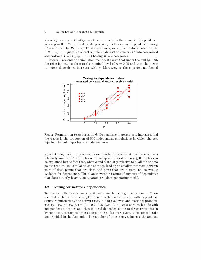
where In is a n × n identity matrix and ρ controls the amount of dependence.When ρ = 0, Y ∗’s are i.i.d. while positive ρ induces some dependence amongY ∗’s informed by W. Since Y ∗ is continuous, we applied cutoffs based on the(0.25, 0.5, 0.75) quantiles of each simulated dataset to convert Y ∗ into categoricalobservations Y = (Y1, Y2, . . . , Yn) having K = 4 categories.

Figure 1 presents the simulation results. It shows that under the null (ρ = 0),the rejection rate is close to the nominal level of α = 0.05 and that the powerto detect dependence increases with ρ. Moreover, as the expected number of

●

●

●

●

●

Teating for dependence in data generated by a spatial autoregressive model

ρ

Pro

port

ion

of r

ejec

ting

the

null

00.

20.

40.

60.

81

0 0.1 0.2 0.3 0.6

●

●

●

●

●

●

●

●

● ●

●

●

●

●

●

●

●

●

●

d=3d=5d=7d=10

Fig. 1: Permutation tests based on Φ. Dependence increases as ρ increases, andthe y-axis is the proportion of 500 independent simulations in which the testrejected the null hypothesis of independence.

adjacent neighbors, d, increases, power tends to increase at fixed ρ when ρ isrelatively small (ρ < 0.6). This relationship is reversed when ρ ≥ 0.6. This canbe explained by the fact that, when ρ and d are large relative to n, all of the datapoints tend to look similar to one another, leading to smaller contrasts betweenpairs of data points that are close and pairs that are distant, i.e. to weakerevidence for dependence. This is an inevitable feature of any test of dependencethat does not rely heavily on a parametric data-generating model.

3.2 Testing for network dependence

To illustrate the performance of Φ, we simulated categorical outcomes Y as-sociated with nodes in a single interconnected network and with dependencestructure informed by the network ties. Y had five levels and marginal probabil-ities (p1, p2, p3, p4, p5) = (0.1, 0.2, 0.3, 0.25, 0.15); we seeded each node withindependent outcomes and then induced dependence due to direct transmissionby running a contagious process across the nodes over several time steps; detailsare provided in the Appendix. The number of time steps, t, indexes the amount


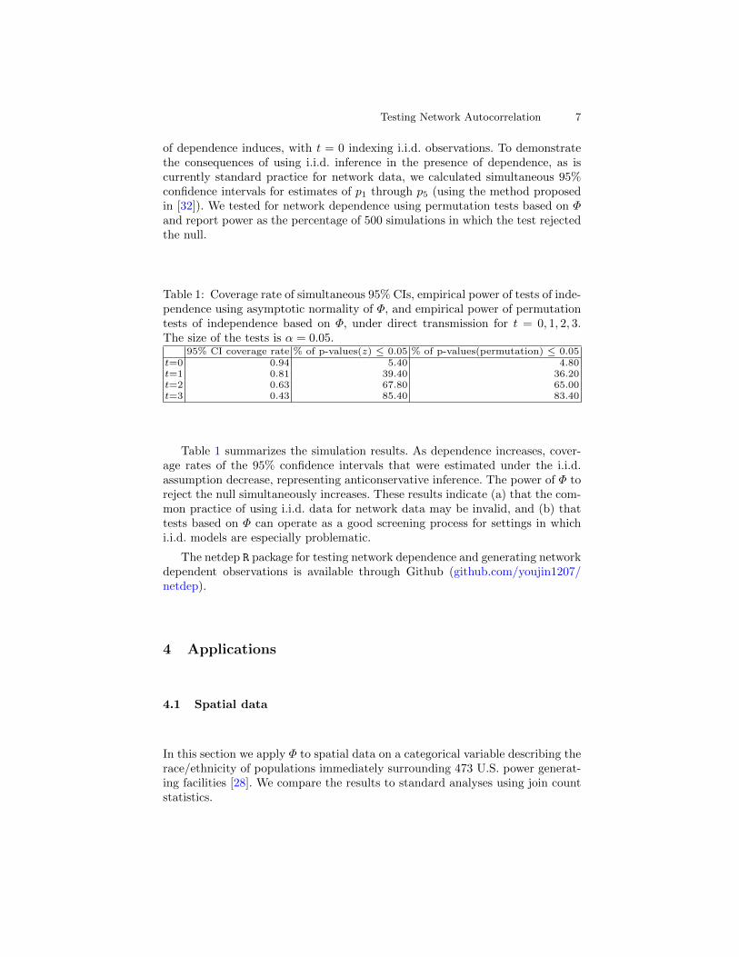
of dependence induces, with t = 0 indexing i.i.d. observations. To demonstratethe consequences of using i.i.d. inference in the presence of dependence, as iscurrently standard practice for network data, we calculated simultaneous 95%confidence intervals for estimates of p1 through p5 (using the method proposedin [32]). We tested for network dependence using permutation tests based on Φand report power as the percentage of 500 simulations in which the test rejectedthe null.

Table 1: Coverage rate of simultaneous 95% CIs, empirical power of tests of inde-pendence using asymptotic normality of Φ, and empirical power of permutationtests of independence based on Φ, under direct transmission for t = 0, 1, 2, 3.The size of the tests is α = 0.05.

95% CI coverage rate % of p-values(z) ≤ 0.05 % of p-values(permutation) ≤ 0.05t=0 0.94 5.40 4.80t=1 0.81 39.40 36.20t=2 0.63 67.80 65.00t=3 0.43 85.40 83.40

Table 1 summarizes the simulation results. As dependence increases, cover-age rates of the 95% confidence intervals that were estimated under the i.i.d.assumption decrease, representing anticonservative inference. The power of Φ toreject the null simultaneously increases. These results indicate (a) that the com-mon practice of using i.i.d. data for network data may be invalid, and (b) thattests based on Φ can operate as a good screening process for settings in whichi.i.d. models are especially problematic.

The netdep R package for testing network dependence and generating networkdependent observations is available through Github (github.com/youjin1207/netdep).

4 Applications

4.1 Spatial data

In this section we apply Φ to spatial data on a categorical variable describing therace/ethnicity of populations immediately surrounding 473 U.S. power generat-ing facilities [28]. We compare the results to standard analyses using join countstatistics.

github.com/youjin1207/netdep

github.com/youjin1207/netdep


●

●●

●●

●●●●

●●

●

●

●●

●

●

●●

●●

●

●●

●●

●

●●●●

●●●●

●

●●

●●

●

●

●●●●

●●

●

●

●

●

●

●

●

●

●●

●●●

●

●

●●●

●

●

●

●

●

●

●

●●●●

●●

●●

●●●

●●●●●●

●●

●

●

●●●

●●

●●

●

●

●●●●

●●

●● ●●

●

●

●

●● ●

●

●●

●

●

●

●

●●

●●

●

●●

●●

●●

●

●●●●

●

●

●

●

●●

●●

●●

● ● ●

●

●●

●●●

●●

●

●●

●

●●

●

●

●●

● ●●●

●●●●

●

●

●●

●

●●●

●

●●

●●●●●●

●●●●

●

●

●●

●

●●

●

●●

●●

●

●●●●●

●●●

●●

●●

●

●

●

●

●

●

●●

●

●●

●

●

●

●

●

●●

●

●

●●

●

●

●

●●

●

●

●

●

●●●●

●

●

●

●

●●

●

●

●

●

●

●

●●

●

●●

●

●

●

●

●

●

●

●

●

●

●

●

●

●

●

●

●

●

●

●●

●

●

●

●

●

●

●

●

●

●

●

●

●

●

● ●

● ●

●●

●

●

●

●

●

●

●

●

●

●

●

●

●

●

●

●

●

●

●

●

●

●

●

●● ●

●

●

●

●

●

●

●

●

●

●●

●

●

●●

●

●

●

●

●

●

●

●

●

●

●●

●

●

●

●

●●●

●

●

●

●

●

●●

●

●

●

●

●

●

●

●

●

●

●

●

●

●

●

●

●

●

●

● ●

●

●●

●

●

●

●

●●

●

●

●

●

●

●

●

●

●

●

●

●

●●

●

●●

●

●

●

●

●●

●

●

●●

●

●

●

●

●

●

●

●

●

●

●●●

●

●

●●

●

●

●

●

●●

●●

●

●●

●

Moran's I: 30.99P−value (permutation) < 0.01

White

●

●●

●●

●●●●

●●

●

●

●●

●

●

●●

●●

●

●●

●●

●

●●●●

●●●●

●

●●

●●

●

●

●●●●

●●

●

●

●

●

●

●

●

●

●●

●●●

●

●

●●●

●

●

●

●

●

●

●

●●●●

●●

●●

●●●

●●●●●●

●●

●

●

●●●

●●

●●

●

●

●●●●

●●

●● ●●

●

●

●

●● ●

●

●●

●

●

●

●

●●

●●

●

●●

●●

●●

●

●●●●

●

●

●

●

●●

●●

●●

● ● ●

●

●●

●●●

●●

●

●●

●

●●

●

●

●●

● ●●●

●●●●

●

●

●●

●

●●●

●

●●

●●●●●●

●●●●

●

●

●●

●

●●

●

●●

●●

●

●●●●●

●●●

●●

●●

●

●

●

●

●

●

●●

●

●●

●

●

●

●

●

●●

●

●

●●

●

●

●

●●

●

●

●

●

●●●●

●

●

●

●

●●

●

●

●

●

●

●

●●

●

●●

●

●

●

●

●

●

●

●

●

●

●

●

●

●

●

●

●

●

●

●●

●

●

●

●

●

●

●

●

●

●

●

●

●

●

● ●

● ●

●●

●

●

●

●

●

●

●

●

●

●

●

●

●

●

●

●

●

●

●

●

●

●

●

●● ●

●

●

●

●

●

●

●

●

●

●●

●

●

●●

●

●

●

●

●

●

●

●

●

●

●●

●

●

●

●

●●●

●

●

●

●

●

●●

●

●

●

●

●

●

●

●

●

●

●

●

●

●

●

●

●

●

●

● ●

●

●●

●

●

●

●

●●

●

●

●

●

●

●

●

●

●

●

●

●

●●

●

●●

●

●

●

●

●●

●

●

●●

●

●

●

●

●

●

●

●

●

●

●●●

●

●

●●

●

●

●

●

●●

●●

●

●●

●


Hispanic

●

●●

●●

●●●●

●●

●

●

●●

●

●

●●

●●

●

●●

●●

●

●●●●

●●●●

●

●●

●●

●

●

●●●●

●●

●

●

●

●

●

●

●

●

●●

●●●

●

●

●●●

●

●

●

●

●

●

●

●●●●

●●

●●

●●●

●●●●●●

●●

●

●

●●●

●●

●●

●

●

●●●●

●●

●● ●●

●

●

●

●● ●

●

●●

●

●

●

●

●●

●●

●

●●

●●

●●

●

●●●●

●

●

●

●

●●

●●

●●

● ● ●

●

●●

●●●

●●

●

●●

●

●●

●

●

●●

● ●●●

●●●●

●

●

●●

●

●●●

●

●●

●●●●●●

●●●●

●

●

●●

●

●●

●

●●

●●

●

●●●●●

●●●

●●

●●

●

●

●

●

●

●

●●

●

●●

●

●

●

●

●

●●

●

●

●●

●

●

●

●●

●

●

●

●

●●●●

●

●

●

●

●●

●

●

●

●

●

●

●●

●

●●

●

●

●

●

●

●

●

●

●

●

●

●

●

●

●

●

●

●

●

●●

●

●

●

●

●

●

●

●

●

●

●

●

●

●

● ●

● ●

●●

●

●

●

●

●

●

●

●

●

●

●

●

●

●

●

●

●

●

●

●

●

●

●

●● ●

●

●

●

●

●

●

●

●

●

●●

●

●

●●

●

●

●

●

●

●

●

●

●

●

●●

●

●

●

●

●●●

●

●

●

●

●

●●

●

●

●

●

●

●

●

●

●

●

●

●

●

●

●

●

●

●

●

● ●

●

●●

●

●

●

●

●●

●

●

●

●

●

●

●

●

●

●

●

●

●●

●

●●

●

●

●

●

●●

●

●

●●

●

●

●

●

●

●

●

●

●

●

●●●

●

●

●●

●

●

●

●

●●

●●

●

●●

●


African American

0.20.40.60.81.0

(a)

●

●●

●●

●●●●

●●

●

●

●●

●

●

●●

●●

●

●●

●●

●

●●●●

●●●●

●

●●

●●

●

●

●●●●

●●

●

●

●

●

●

●

●

●

●●

●●●

●

●

●●●

●

●

●

●

●

●

●

●●●●

●●

●●

●●●

●●●●●●

●●

●

●

●●●

●●

●●

●

●

●●●●

●●

●● ●●

●

●

●

●● ●

●

●●

●

●

●

●

●●

●●

●

●●

●●

●●

●

●●

●●

●

●

●

●

●●

●●

●●

● ● ●

●

●●

●●●

●●

●

●●

●

●●

●

●

●●

● ●●●

●●●●

●

●

●●

●

●●●

●

●●

●●●●●●

●●●

●

●

●

●●

●

●●

●

●●

●●

●

●●●●●

●●●

●●

●●

●

●

●

●

●

●

●●

●

●●

●

●

●

●

●

●●

●

●

●●

●

●

●

●●

●

●

●

●

●●●●

●

●

●

●

●●

●

●

●

●

●

●

●●

●

●●

●

●

●

●

●

●

●

●

●

●

●

●

●

●

●

●

●

●

●

●●

●

●

●

●

●

●

●

●

●

●

●

●

●

●

● ●

● ●

●●

●

●

●

●

●

●

●

●

●

●

●

●

●

●

●

●

●

●

●

●

●

●

●

●● ●

●

●

●

●

●

●

●

●

●

●●

●

●

●●

●

●

●

●

●

●

●

●

●

●

●●

●

●

●

●

●●●

●

●

●

●

●

●●

●

●

●

●

●

●

●

●

●

●

●

●

●

●

●

●

●

●

●

● ●

●

●●

●

●

●

●

●●

●

●

●

●

●

●

●

●

●

●

●

●

●●

●

●●

●

●

●

●

●●

●

●

●●

●

●

●

●

●

●

●

●

●

●

●●●

●

●

●●

●

●

●

●

●●

●●

●

●●

●

Φ: 9.17P−value (permutation) < 0.01

●

●

●

WhiteHispanicAfrican−American

Most populous group

●

●●

●●

●●●●

●●

●

●

●●

●

●

●●

●●

●

●●

●●

●

●●●●

●●●●

●

●●

●●

●

●

●●●●

●●

●

●

●

●

●

●

●

●

●●

●●●

●

●

●●●

●

●

●

●

●

●

●

●●●●

●●

●●

●●●

●●●●●●

●●

●

●

●●●

●●

●●

●

●

●●●●

●●

●● ●●

●

●

●

●● ●

●

●●

●

●

●

●

●●

●●

●

●●

●●

●●

●

●●

●●

●

●

●

●

●●

●●

●●

● ● ●

●

●●

●●●

●●

●

●●

●

●●

●

●

●●

● ●●●

●●●●

●

●

●●

●

●●●

●

●●

●●●●●●

●●●

●

●

●

●●

●

●●

●

●●

●●

●

●●●●●

●●●

●●

●●

●

●

●

●

●

●

●●

●

●●

●

●

●

●

●

●●

●

●

●●

●

●

●

●●

●

●

●

●

●●●●

●

●

●

●

●●

●

●

●

●

●

●

●●

●

●●

●

●

●

●

●

●

●

●

●

●

●

●

●

●

●

●

●

●

●

●●

●

●

●

●

●

●

●

●

●

●

●

●

●

●

● ●

● ●

●●

●

●

●

●

●

●

●

●

●

●

●

●

●

●

●

●

●

●

●

●

●

●

●

●● ●

●

●

●

●

●

●

●

●

●

●●

●

●

●●

●

●

●

●

●

●

●

●

●

●

●●

●

●

●

●

●●●

●

●

●

●

●

●●

●

●

●

●

●

●

●

●

●

●

●

●

●

●

●

●

●

●

●

● ●

●

●●

●

●

●

●

●●

●

●

●

●

●

●

●

●

●

●

●

●

●●

●

●●

●

●

●

●

●●

●

●

●●

●

●

●

●

●

●

●

●

●

●

●●●

●

●

●●

●

●

●

●

●●

●●

●

●●

●

Φ: 22.72P−value (permutation) < 0.01

●

●

●

●

AA > 10 % & HP > 10 %AA > 10 % & HP <= 10 %AA <= 10 % & HP > 10 %AA <= 10 % & HP <= 10 %

Hispanic and African American populations

(b)

Fig. 2: Panel (a): Proportion of race/ethnicity groups around 473 power-producing facilities across the U.S.. Applying Moran’s I separately to each pro-portion, all of the tests reject the null hypothesis of independence at the α = 0.05level. Panel (b) : Most populous group (left) and categories defined by having≤10% or >10% Hispanic or African American residents (right). Omnibus testsof dependence based on Φ reject the null hypothesis of independence at theα = 0.05 level for both variables.

Figure 2a depicts the composition of the population living within a 100 kmradius of each power generating facility, with the shade of each dot represent-ing the proportion of the population falling into each race/ethnicity category(White/Hispanic/African American). We can apply Moran’s I separately to dataon each of the three categories, but Moran’s I cannot provide a single aggregatetest statistic. Figure 2b depicts the distributions of two alternative categoricalsummaries of the information from Figure 2a: a 3-level variable indicating themost populous group in the area surrounding each facility, and a 4-level variableindicating whether more than 10% of the population is Hispanic and AfricanAmerican, respectively. Using each of these categorial variables, we can performan omnibus test for dependence using Φ. We observe greater evidence of de-pendence in the second categorization (Φ : 22.72) than the first categorization(Φ : 9.17). This direct comparison is possible using Φ but would not be possibleusing join count statistics. The join count statistics for these two categoricalvariables are given in Table 2 and Table 3. The statistics themselves count thefrequency of concordant neighboring pairs for each category and standardize it;the p-values are derived from a permutation test that permutes the location ofeach observation while holding the values fixed. Join count analysis requires anotion of adjacency; we specified a neighborhood size of 15, meaning that obser-


vation j is considered to be adjacent to i if j is one of i’s closet 15 neighbors inEuclidean distance.

Table 2: Permutation tests of dependence based on join count statistics appliedto the most populous group.

Most populous group White Hispanic African-American

n 446 13 14Join count statistic 212.63 0.97 0.77P-value (permutation) < 0.01 < 0.01 < 0.01

Table 3: Permutation tests of dependence based on join count statistics ap-plied to four different population categories, defined by having ≤10% or >10%Hispanic or African American residents.

AA > 10%, HP > 10% AA > 10%, HP ≤ 10% AA ≤ 10%, HP > 10% AA ≤ 10%, HP ≤ 10%

n 52 106 98 217Join-count statistic 7.07 26.63 30.30 69.20

P-value (permutation) < 0.01 < 0.01 < 0.01 < 0.01

4.2 Network data

The Framingham Heart Study, initiated in 1948, is an ongoing cohort study ofparticipants from the town of Framingham, Massachusetts that was originallydesigned to identify risk factors for cardiovascular disease. The study has grownover the years to include five cohorts. For decades, FHS has been one of themost successful and influential epidemiologic cohort studies in existence. It isarguably the most important source of data on cardiovascular epidemiology.It has been analyzed using i.i.d. statistical models (as is standard practice forcohort studies) in over 3,400 peer-reviewed publications since 1950: to studycardiovascular disease etiology (e.g. [2, 7]), risks for developing obesity (e.g. [34]),factors affecting mental health (e.g. [29, 30]), and many other outcomes.

In addition to being a very prominent cohort study, more recently FHS hasplayed a uniquely influential role in the study of social networks and socialcontagion. Researchers reconstructed the (partial) social network underlying thecohort and used this network to study social contagion and peer influence for avariety of outcomes in a series of highly influential papers [3, 4, 11]. However, eventhese analyses use methods that assume independence across subjects [22, 16].In a companion paper we test for dependence in continuous and binary variablesin the FHS data, and discuss the implications of network dependence for thebody of research that relies on i.i.d. analyses these data. Here we illustrate thatdependence in these data may extend beyond continuous and binary variables


to categorical variables, which previous methods would not have been able toascertain. We analyzed n =1,033 subjects with 690 undirected social networkties from the Offspring Cohort at Exam 5, which was conducted between 1991and 1995.

Employment status

●

●

●

●

●●

●●

●

●

●

●●

●

●

●

●●

●

●

●

●

●●

●

●

●

●

●

●

●

●

●

●

●

●●

●

●

●

●●

●

●

●

●

●

●

●●

●

●

●

●

●

●

●

●

●

●

●

●

●

●

●

●

●

●

●

●●

●

●

●

●

● ●

●

●

●

●

●

●●

●

●

●

●

●

●●

●●

●

●

●

●

●

●

●

●

●

●

●

●

●

●●●

●

●

●

●

●

●

●●

●

●●

●

●

●

●

●

●

●

●

●●

●

●

●

●

●●

●

●

●

●

●

●

●

●

●

●●

●

●●

● ●

●

●

●●

●

●

Φ: 3.40p−value (permutation) < 0.01

●

●

●

FulltimeParttimeNot employed

Ways to make coffee

●

●

●

●

●

●

●●

●

●

●

●

●

●

●

●

●

●

●

●

●

●

●

●

●

●

●

●

●

●

●

●

●

●

●

●

●

●

●●

●

●

●

●

●

●

●●

●

●

●

●●

●

●●

●

●

●

●

●

●

●

●

●

●

●

●

●

●

●●

●

●

●

●

●

●

●

●

●

●

●

●●

●

●●

●

●

●

●

●●

●

●

●

●

●

●

●

●

●

●

●

●

●

●

●

●

●

●

●

●

●

●

●

●●

●

●●

●

●

●

●

●

●

●

●

●●

●

●

●

●

●

●

●

●

●

●

●

●

●

●

●

●

●

●

●

●

●

●

●

●

●

●

●

●

Φ: 3.21p−value (permutation) < 0.01

●

●

●

●

Non−drinkerFilterPercInstant

Fig. 3: Network dependence test for categorical variables with three levels (left)and four levels (right) using Φ.

We tested for dependence in two different categorical random variables usingΦ: employment status and preferred method of making coffee. Figure 3 showsthe distribution of these two variables over the largest connected componentof the network. We found significant evidence of network dependence for bothvariables, resulting p-value of < 0.01 in both variables.

5 Concluding Remarks

In this paper, we proposed a simple test for dependence among categorical obser-vations sampled from geographic space or from a network. We demonstrated theperformance of our proposed test in simulations under both spatial and networkdependence, and applied it to spatial data on U.S. power producing facilitiesand to social network data from the Framingham Heart Study.

Under network dependence, adjacent pairs are expected to exhibit the great-est correlations, and for robustness we used the adjacency matrix as the weightmatrix for calculating the test statistic, thereby restricting our analysis to adja-cent pairs; if researchers have substantive knowledge of the dependence mecha-nism other weights may increase power and efficiency.

Researchers should be aware of the possibility of dependence in their observa-tions, both when studying social networks explicitly and when observations aresampled from a single community for reasons of convenience. As we have seen


in the classic Framingham Heart Study example, such observations can be de-pendence, potentially rendering i.i.d. statistical methods invalid. In a companionpaper [16], we delve deeper into the consequences of assuming that observationsare independent when they may in fact exhibit network dependence. That paperfocuses on continuous and binary variables, but similar conclusions hold for thecategorical variables that we addressed in this paper.

Acknowledgments

Youjin Lee and Elizabeth Ogburn were supported by ONR grant N000141512343.The Framingham Heart Study is conducted and supported by the NationalHeart, Lung, and Blood Institute (NHLBI) in collaboration with Boston Univer-sity (Contract No. N01-HC-25195 and HHSN268201500001I). This manuscriptwas not prepared in collaboration with investigators of the Framingham HeartStudy and does not necessarily reflect the opinions or views of the FraminghamHeart Study, Boston University, or NHLBI.

A Appendix

A.1 Moments of Φ

Here we derive µΦ := E[Φ] and E[Φ2], the first and second moments of Φ.Based on these moments, we can derive the variance of Φ, σ2

Φ := E[Φ2] − µ2Φ.

When K is the number of categories and pj is the proportion of Y in categoryj (j = 1, 2, . . . ,K),

µΦ =1

n(n− 1){n2K(2− k)− nQ1},

E[Φ2] =1

S20

[S1

n(n− 1)(n2Q22 − nQ3)

+S2 − 2S1

n(n− 1)(n− 2)((K − 4)K + 4)n3Q1 + n(n((2K − 4)Q2 −Q22) + 2Q3)

+S20 − S2 + S1

n(n− 1)(n− 2)(n− 3)

{n(−4Q3 + 2nQ22 − 6KnQ2 + 12nQ2

− 3K2n2Q1 + 14Kn2Q1 − 16n2Q1 +K4n3 − 4K3n3 + 4K2n3)

− ((2K − 4)n2Q2 + n2(Kn(2Q1 −KQ1)−Q22) + 2nQ3)}],

(3)

where Qm :=K∑l=1

1/pml , (m = 1, 2, 3); Q22 :=K∑l=1

K∑u=1

1/plpu ; S0 =n∑i=1

n∑j=1

(wij +

wji)/2; S1 =n∑i=1

n∑j=1

(wij + wji)2/2; S2 =

n∑i=1

(wi· + w·i)2.


A.2 Asymptotic distribution of Φ under the null

Shapiro and Hubert [31] proved the asymptotic normality of permutation statis-tics of the form Hn for i.i.d. random variables Y1, Y2, . . . , Yn under some condi-tions:

Hn =

n∑i=1

n∑j=1,j 6=i

dijh(Yi, Yj), (4)

where h(·, ·) is a symmetric real valued function with E[h2(Yi, Yj)] <∞ and D :={dij ; i, j = 1, ..., n} is a n × n symmetric, nonzero matrix of which all diagonalterms must be zero. In the context of Φ, h(Yi, Yj) =

(2I(Yi = Yj)− 1

)/(pYi

pYj)

and D = W. Requirements for asymptotic normality includen∑

i,j=1,j 6=id2ij/

n∑i=1

d2i· →

0 and max1≤i≤n

d2i·/n∑k=1

d2k· → 0 as n → 0 for di· =n∑j=1

dij . If we use the adjacency

matrix for W, this impliesn∑

i,j=1,i6=jAij/

n∑i=1

A2i· → 0 and max

1≤i≤nAi·/

n∑i=1

A2i· → 0

where Ai· is the degree of node i. More details can be found in [31]; see also [25].

B Simulation of categorical observations over network

B.1 Direct transmission simulations

We specify the starting probability that each observation falls into one of K

categories, {(p1, p2, ..., pK) :K∑j=1

pk = 1}. We then simulate initial outcomes from

a multinomial distribution, and generate outcomes at subsequent time pointsiteratively:

Y 01 , Y

02 , . . . , Y

0ni.i.d∼ Multinomial

((p1, p2, . . . , pK)

)Y ti =

{Zti ∼ Multinomial

((pt−1i1 , pt−1i2 , . . . , pt−1iK )

)with probability q

Y t−1i with probability 1− q(5)

where pt−1im :=n∑j=1

wijI(yt−1j = m)/n∑j=1

wij ; m = 1, ..,K; 0 < q ≤ 1. At each

time point, with probability q, a node’s outcome is updated as a draw froma new multinomial with probabilities influenced by the proportion of adjacentnodes falling into each category at the previous time. The amount of influencefrom adjacent peers can be controlled by pre-specified maximum susceptibilityprobability qm(0 ≤ qm ≤ 1), where q ∈ [0, qm], and we set qm = 0.4.

References

[1] Anselin L, Bera AK, Florax R, Yoon MJ (1996) Simple diagnostic tests forspatial dependence. Regional Science and Urban Economics 26(1):77–104

[2] Castelli W (1988) Cholesterol and lipids in the risk of coronary arterydisease–the framingham heart study. The Canadian Journal of Cardiology4:5A–10A

[3] Christakis NA, Fowler JH (2007) The spread of obesity in a large socialnetwork over 32 years. New England Journal of Medicine 357(4):370–379

[4] Christakis NA, Fowler JH (2008) The collective dynamics of smoking in alarge social network. New England Journal of Medicine 358(21):2249–2258

[5] Cliff A, Ord K (1972) Testing for spatial autocorrelation among regressionresiduals. Geographical Analysis 4(3):267–284

[6] Cliff AD, Ord K (1970) Spatial autocorrelation: a review of existing andnew measures with applications. Economic Geography 46(sup1):269–292

[7] D’Agostino RB, Vasan RS, Pencina MJ, Wolf PA, Cobain M, Massaro JM,Kannel WB (2008) General cardiovascular risk profile for use in primarycare the framingham heart study. Circulation 117(6):743–753

[8] Diniz-Filho JAF, Bini LM, Hawkins BA (2003) Spatial autocorrelationand red herrings in geographical ecology. Global ecology and Biogeography12(1):53–64

[9] Farber S, Paez A, Volz E (2009) Topology and dependency tests in spatialand network autoregressive models. Geographical Analysis 41(2):158–180

[10] Farber S, Marin MR, Paez A (2015) Testing for spatial independence usingsimilarity relations. Geographical Analysis 47(2):97–120

[11] Fowler JH, Christakis NA (2008) Dynamic spread of happiness in a largesocial network: longitudinal analysis over 20 years in the framingham heartstudy. Bmj 337:a2338

[12] Fujimoto K, Chou CP, Valente TW (2011) The network autocorrelationmodel using two-mode data: Affiliation exposure and potential bias in theautocorrelation parameter. Social Networks 33(3):231–243

[13] Geary RC (1954) The contiguity ratio and statistical mapping. The Incor-porated Statistician 5(3):115–146

[14] Griffith DA (2000) A linear regression solution to the spatial autocorrelationproblem. Journal of Geographical Systems 2(2):141–156

[15] Kossinets G, Watts DJ (2006) Empirical analysis of an evolving social net-work. Science 311(5757):88–90

[16] Lee Y, Ogburn EL (2019) Network dependence and confounding by networkstructure lead to invalid inference. arXiv preprint ArXiv:1908.00520

[17] Legendre P (1993) Spatial autocorrelation: trouble or new paradigm? Ecol-ogy 74(6):1659–1673

[18] Lennon JJ (2000) Red-shifts and red herrings in geographical ecology. Ecog-raphy 23(1):101–113


[19] Lewis K, Kaufman J, Gonzalez M, Wimmer A, Christakis N (2008) Tastes,ties, and time: A new social network dataset using facebook.com. SocialNetworks 30(4):330–342

[20] Lichstein JW, Simons TR, Shriner SA, Franzreb KE (2002) Spatial auto-correlation and autoregressive models in ecology. Ecological Monographs72(3):445–463

[21] Long J, Harre N, Atkinson QD (2015) Social clustering in high school trans-port choices. Journal of Environmental Psychology 41:155–165

[22] Lyons R (2011) The spread of evidence-poor medicine via flawed social-network analysis. Statistics, Politics, and Policy 2(1):126

[23] Moran PA (1948) The interpretation of statistical maps. Journal of theRoyal Statistical Society Series B (Methodological) 10(2):243–251

[24] Ogburn EL (2017) Challenges to estimating contagion effects from obser-vational data. arXiv preprint ArXiv:1706.08440

[25] O’Neil KA, Redner RA (1993) Asymptotic distributions of weighted u-statistics of degree 2. The Annals of Probability pp 1159–1169

[26] Ord JK, Getis A (1995) Local spatial autocorrelation statistics: distribu-tional issues and an application. Geographical Analysis 27(4):286–306

[27] Overmars Kd, De Koning G, Veldkamp A (2003) Spatial autocorrelation inmulti-scale land use models. Ecological Modelling 164(2):257–270

[28] Papadogeorgou G, Choirat C, Zigler CM (2018) Adjusting for unmeasuredspatial confounding with distance adjusted propensity score matching. Bio-statistics 20(2):256–272

[29] Qiu WQ, Dean M, Liu T, George L, Gann M, Cohen J, Bruce ML (2010)Physical and mental health of homebound older adults: an overlooked pop-ulation. Journal of the American Geriatrics Society 58(12):2423–2428

[30] Saczynski JS, Beiser A, Seshadri S, Auerbach S, Wolf P, Au R (2010) De-pressive symptoms and risk of dementia the framingham heart study. Neu-rology 75(1):35–41

[31] Shapiro CP, Hubert L, et al (1979) Asymptotic normality of permutationstatistics derived from weighted sums of bivariate functions. The Annals ofStatistics 7(4):788–794

[32] Sison CP, Glaz J (1995) Simultaneous confidence intervals and sample sizedetermination for multinomial proportions. Journal of the American Statis-tical Association 90(429):366–369

[33] Smouse PE, Peakall R (1999) Spatial autocorrelation analysis of individualmultiallele and multilocus genetic structure. Heredity 82(5):561–573

[34] Vasan RS, Pencina MJ, Cobain M, Freiberg MS, D’Agostino RB (2005) Es-timated risks for developing obesity in the framingham heart study. Annalsof Internal Medicine 143(7):473–480

[35] Weaver IS, Williams H, Cioroianu I, Williams M, Coan T, Banducci S (2018)Dynamic social media affiliations among uk politicians. Social Networks54:132–144

Testing for Network and Spatial Autocorrelationtesting spatial autocorrelation in categorical...

Documents

Transcript of Testing for Network and Spatial Autocorrelationtesting spatial autocorrelation in categorical...