Testing for Cointegration When Some of the Cointegrating ...mwatson/papers/Horvath... · TESTING...

Econometric Theory, 11, 1995, 984-1014. Printed in the United States of America.

TESTING FOR COINTEGRATION WHEN SOME OF THE

COINTEGRATING VECTORS ARE PRESPECIFIED

MICHAEL T.K. HORVATH Stanford University

MARK W. WATSON Princeton University

Many economic models imply that ratios, simple differences, or "spreads" of variables are I(O). In these models, cointegrating vectors are composed of l's, O's, and - l's and contain no unknown parameters. In this paper, we develop tests for cointegration that can be applied when some of the cointegrating vectors are prespecified under the null or under the alternative hypotheses. These tests are constructed in a vector error correction model and are motivated as Wald tests from a Gaussian version of the model. When all of the cointegrating vectors are prespecified under the alternative, the tests correspond to the standard Wald tests for the inclusion of error correction terms in the VAR. Modifications of this basic test are developed when a subset of the cointegrating vectors contain unknown parameters. The asymptotic null distributions of the statistics are derived, critical values are determined, and the local power properties of the test are studied. Finally, the test is applied to data on foreign exchange future and spot prices to test the stability of the forward-spot premium.

1. INTRODUCTION

Economic models often imply that variables are cointegrated with simple and known cointegrating vectors. Examples include the neoclassical growth model, which implies that income, consumption, investment, and the capi- tal stock will grow in a balanced way, so that any stochastic growth in one of the series must be matched by corresponding growth in the others. Asset

This paper has benefited from helpful comments by Neil Ericsson, Gordon Kemp, Andrew Levin, Soren Johansen, John McDermott, Pierre Perron, Peter Phillips, James Stock, and three referees. This research was supported by grants from the National Science Foundation (SES-91-22463 and SBR-94-09629) and the Sloan Foundation. Address correspondence to: Professor Mark Watson, Woodrow Wilson School, Prince- ton University, Princeton, NJ 08540, USA.

984 ? 1995 Cambridge University Press 0266-4666/95 $9.00 + .10

TESTING WITH PRESPECIFIED COINTEGRATING VECTORS 985

pricing models with stable risk premia imply corresponding stable differences in spot and forward prices, long- and short-term interest rates, and the logarithms of stock prices and dividends. Most theories of international trade imply long-run purchasing power parity, so that long-run movements in nominal exchange rates are matched by countries' relative price levels. Certain monetarist propositions are centered around the stability of velocity, imply- ing cointegration among the logarithms of money, prices, and income. Each of these theories has two distinct implications for the properties of economic time series under study: first, the series are cointegrated, and second, the cointegrating vector takes on a specific value. For example, balanced growth implies that the logarithms of income and consumption are cointegrated and that the cointegrating vector takes on the value of (1 -1).

The most widely used approach to testing these cointegration propositions is articulated and implemented in Johansen and Juselius (1992), who investigate the empirical support for long-run purchasing power parity. They implement a two-stage testing procedure. In the first stage, the null hypothesis of no cointegration is tested against the alternative that the data are cointegrated with an unknown cointegrating vector using Johansen's (1988) test for cointegration. If the null hypothesis is rejected, a second stage test is implemented with cointegration maintained under both the null and alternative. The null hypothesis is that the data are cointegrated with the specific cointegrating vector implied by the relevant economic theory ([1 -1] in the consumption-income example), and the alternative is that data are cointegrated with another unspecified cointegrating vector. Because a consistent test for cointegration is used in the first stage, potential cointegration in the data is found with probability approaching 1 in large samples. Thus, the probability of rejecting the cointegration constraints on the data imposed by the economic model are given by the size of the test in the second step, at least in large samples. An important strength of this procedure is that it can uncover cointegration in the data with a cointegrating vector different from the cointegrating vector imposed by the theory. The disadvantage is that the sample sizes used in economics are often relatively small, so that the first- stage tests may have low power.

This paper discusses an alternative procedure in which the null of no cointegration is tested against the composite alternative of cointegration using a prespecified cointegrating vector. This approach has two advantages. First, and most important, the resulting test for cointegration is significantly more powerful than the test that does not impose the cointegrating vector. For example, in the bivariate example analyzed in Section 3, these power gains correspond to sample size increases ranging from 40 to 70Wo for a test with power equal to 5Oo. The second advantage is that the test statistic is very easy to calculate: it is the standard Wald test for the presence of the candi- date error correction terms in the first difference vector autoregression. The countervailing disadvantage of the testing approach is that it does not sep-

986 MICHAEL T.K. HORVATH AND MARK W. WATSON

arate the two components of the alternative hypothesis and, thus, may fail to reject the null of no cointegration when the data are cointegrated with a cointegrating vector different from that used to construct the test. We investigate this in Section 3, where it is shown that in situations with weak cointegration (represented by a local-to-unity error correction term) even inexact information on the value of the cointegrating vector often leads to power im- provements over the test that uses no information. If the null hypothesis of noncointegration is rejected, one can then determine whether the prespecified cointegrating vector differs significantly from the true cointegrating vector.

The plan of this paper is as follows. In Section 2, we consider the general problem of testing for cointegration in a model in which some of the potential cointegrating vectors are known, and some are unknown, under both the null and the alternative. In particular, we present Wald and likelihood ratio tests for the hypothesis that the data are cointegrated with rOk known and r0u unknown cointegrating vectors under the null. Under the alternative, there are rak and rau additional known and unknown cointegrating vectors, respectively. The tests are constructed in the context of a finite-order Gauss- ian vector error correction model (VECM) and generalize the procedures of Johansen (1988), who considered the hypothesis testing problem with rOk = rak = 0. In Section 2, we also derive the asymptotic null distributions of the test statistics and tabulate critical values. Section 3 focuses on the power properties of the test. First, we present comparisons of the power of likelihood-based tests that do and do not use information about the value of the cointegrating vector. Next, because information about the potential cointegrating vector might be inexact, we investigate the power loss associated with using an incorrect value of the cointegrating vector. Finally, when there are no cointegrating vectors under the null and only one cointegrating vector under the alternative, simple univariate unit root tests provide an alternative to the multivariate VECM-based tests. Section 3 compares the power of these univariate unit root tests to the multivariate VECM-based tests. Sec- tion 4 contains an empirical application that investigates the forward premia in foreign exchange markets by examining the cointegration properties of forward and spot prices. Section 5 contains some concluding remarks.

2. TESTING FOR COINTEGRATION IN THE GAUSSIAN VAR MODEL

As in Johansen (1988), we derive tests for cointegration in the context of the reduced rank Gaussian VAR:

Yt= dt + Xt, (2.1a)

p

Xt = E HiXt-i + Et, (2.1b) i-l1


where Y, is an n x 1 data vector from a sample of size T, dt represents deterministic drift in Y,, Xt is an n x 1 random vector generated by (2. lb), (, is NIID(0,Ee), and, for convenience, the initial conditions X_i, i = 0,. ..p, are assumed to equal 0. To focus attention on the long-run behavior of the process, it is useful to rewrite (2.lb) as

p-i

AXt = llX,_1 + E i 4AXt- + ,t, (2.1c) i=l

where 1 = -In + I'1 Hi. Our interest is focused on r = rank(IH), and we consider tests of the

hypothesis

Ho: rank (I) = r = r,

Ha: rank(II) = r = rO + r, with r, > 0.

The alternative is written so that ra represents the number of additional cointegrating vectors that are present under the alternative. We assume that ro = rOk + ro, where rOk is the number of cointegrating vectors that are known under the null and ro, represents the number of cointegrating vectors that are unknown (or, alternatively, unrestricted) under the null. Similarly, ra = rak + ra, where the subscripts k and u denote known and unknown, respectively. The rOk prespecified vectors are thought to be cointegrating vectors under the alternative; under the null, they do not cointegrate the series. In spite of this, for expositional ease, they will be referred to as cointegrating vectors.

As in Engle and Granger (1987), Johansen (1988), and Ahn and Reinsel (1990), it is convenient to write the model in vector error correction form by factoring the matrix HI as H = 6a', where 6 and a are n x r matrices of full column rank and the columns of ca denote the cointegrating vectors. The columns of a are partitioned as a = (aoO aa), where a,o is an n x ro matrix whose columns are the cointegrating vectors present under the null, Ola is an n x ra matrix whose columns are the additional cointegrating vectors present uiider the alternative. The matrix 6 is partitioned conformably as 6 = (6b 6a),

where 60 is n x ro and 6a is n x ra. It is also useful to partition cia to isolate the known and unknown cointegrating vectors. Thus, ?a = (ciak dau), where the rak columns of aak are the additional cointegrating vectors known under the alternative, and the rau columns of a - are the additional cointegrating vectors that are present but unrestricted under the alternative. The matrix 6a iS partitioned conformably as 6a = (6Oak au) Using this notation, IIX,_1 = 6o (aO'Xt- 1) + 6a (CaXt- 1), and the competing hypotheses are Ho : 6, = 0 vs. Ha: 6a 0, with rank(6,a') = ra.

We develop tests for Ho vs. Ha in three steps. First, we abstract from deterministic components and derive the likelihood ratio statistic and some useful asymptotically equivalent statistics under the maintained assumption


that dt = 0. Second, we discuss how these statistics can be modified for nonzero values of d,. Finally, the asymptotic null distributions of the resulting statistics are derived and critical values based on these asymptotic distributions are tabulated.

2.1. Calculating the LR and Wald Test Statistics When dt = 0

The likelihood ratio statistic for testing Ho : r = rOk + r0, vs. Ha: r = rOk + rak + r0U + r0a will depend on rOk, rak, ro,, ra and the values of Xo, and (yak. We write the statistic as LRrO,ra(fYokoaak). The values of rOk and rak appear implicitly as the ranks of a1ok and c0ak, respectively. When rOk = 0, the statistic is written as LRro,ra(0,aak) and as LRro,ra(xaok,O) when ra, = 0.

To derive the LR statistic, we limit attention to the problem with ro = rOk = ro, = 0. For the purposes of deriving the computational formula for the LR statistic, this is without loss of generality because, in the general case, the LR statistic is identically

LRro,ra (a0k Olak) LRo,ro+ra (0, Ika0k]) - LRO0ro (0, ?Yk)' (2.2)

With ro = 0, and ignoring the deterministic components, dt, the model can be written as

AYt = 6ak(aakYt-1) + 6a,,(aa,,Yt-I) + /3Zt + Et, (2.3)

where f3 = (41 42 * ' * p-4 I) and Zt = (A Yt_AY2 I A * AYP+1)' In the context of (2.3), the null hypothesis Ho: r = 0 can be written as the composite null Ho:60k =0, ?au = 0.1 It is convenient to discuss each part of this null separately: we first consider testing bak = 0 maintaining bau = 0, then the converse, and finally the joint hypothesis.

The test statistic for Ho: r = 0 vs. Ha: r = rak. When rau = 0, equation (2.3) simplifies to

Yt = bak(ta .yt-l) + fZt + et' (2.4)

Because ca'kY,_ does not depend on unknown parameters, (2.4) is a standard multivariate linear regression, so that the LR, Wald, and LM statistics have their standard regression form. Letting Y = [Y1 Y2 ... YT]', Y-1 =

[YOYI ... YT-1]', AY= Y- Y-1, Z = [Zl Z2 . . . ZT], e = [E162 * * ET], and Mz = [I - Z(Z'Z)' Z'], the ordinary least-squares (OLS) estimator of 60k is 6ak = (i\YMzY1ogk)( kY_LMzY_ctGk), which corresponds to the Gaussian maximum likelihood estimate (MLE). The corresponding Wald test statistic for H0 vs. Ha is

W = [vec(60k)] [ ()kY- MZY_ Iak) (0 NEJ][vec(6ak)]

= [vec(A Y'MzY_ I cak)]' [(cakY'I MZY-lIaak) ]

x [vec(AY'MzY_laak)], (2.5)


where Se is the usual estimator value of E, that is, E, = T' E -, and where e is the matrix of OLS residuals from (2.4). For values of 60ck that are T` local to 60k = 0, the LR and LM statistics are asymptotically equal to W.

The test statisticfor Ho: r = O vs. Ha: r = r0,. The model simplifies to (2.4) with bau and aau replacing 6,k and cgak. However, the analog of the Wald statistic in (2.5) cannot be calculated because the regressor ?a 'Y-1 depends on unknown parameters. However, the LR statistic can be calculated, and useful formulae for the LR statistic are developed in Anderson (1951) and Johansen (1988). Because bau = 0 under the null hypothesis, the cointegrating vectors cxau are unidentified, and this complicates the testing problem in ways familiar from the work of Davies (1977, 1987). The problem can be avoided when ra = n, because in this case II is unrestricted under the alternative and the null and alternative become Ho : H = 0 vs. Ha: H I 0. The problem cannot be avoided when the rank(II) < n under the alternative. Indeed, in the standard classical reduced rank regression, the general form of the asymptotic distribution of the LR statistic has only been derived for the case in which the matrix of regression coefficients has full rank under the alternative. In this case, Anderson (1951) shows that the LR statistic has an asymptotic x2 null distribution. When the matrix of regression coefficients has reduced rank under the alternative, the asymptotic distribution of the LR statistic depends on the distribution of the regressors. Still, the special struc- ture of the regressors in the cointegrated VAR allows Johansen (1988) to cir- cumvent this problem and derive the asymptotic distribution of the LR test even when II has reduced rank under the alternative.

As pointed out by Hansen (1990), when some parameters are unidentified under the null, the LR statistic can be interpreted as a maximized version of the Wald statistic. This interpretation is useful here because it suggests a simple way to compute the statistic. Because this form of the statistic appears as one component in the test statistic for the general ra = rak + rau alternative, we derive it here.

Let LR denote the likelihood ratio statistic for testing Ho versus Ha, and let LR*( E) denote the (infeasible) LR statistic that would be calculated if Se

were known. As usual, LR = LR*( E) + op (1) under Ho and local alternatives (here, T'). Let L (6a oau E,) denote the log likelihood written as a function Of 6ag, cxau, and 1,, with ,B concentrated out, and let 6au(clau) denote the MLE of bau for fixed Oa!. Then, the well-known relation between the Wald and LR statistic in the linear model implies that

W( au ) = 2 [L (bau (aau), au, -e)-L (0, L Cau, eJ)]

= 2[L(b ( ?(a E)Jc ?,,1) -L (0, 0,S)] , (2.6)

where W(aau) is the Wald statistic in (2.5) written as a function of cau; the first equality follows because each log-likelihood function is evaluated using


SE; and the second equality follows because aeau does not enter the likelihood when 6au = 0. Thus,

~~~~~ AA

Sup W(olau) = Sup 2[L(bau(oau),oau,-e) L(O,0,E,)] = LR (,E), xa, xaa,

where the Sup is taken over all n x rau matrices au. To calculate Sup,,0 W(aau), rewrite (2.5) as

W( au) = [vec(AY'MzY_Icau )]'[(au Y'iMZY_i1oau )0

x [vec(AY'MzY_iaau)] A

X (c4aUMz Y_ 1iAY ) e1/2't]

- TR[ e 12(/2 (Y'Mz Y_1 )DD'(MyY'1 )2]

where D = Otau (?au YLI MzY_1 a!au)

- TR[D'(YL'1 MzAY)e ?(AY'MzY1 )D]

- TR[F'CC'F], (2.7)

where F = (Y'LMzYil)1/2ea"(ol Y'LMzYioaa)-'/2 and C = (Y MY1-/(! MiY? /t Notice that F'F = Ira and Supxa W(c?au) =-SUPF'F=ITR[F'( CC' )F] . Let X\i( CC' ) denote the eigenvalues of (CC') ordered so that X1 2 X2 ? '. > Xn Then,

ra

Sup W(cxeau) = Sup TR [F'( CC' )F] = ,j Xi( CC') odal ~F'F=1 i=1l

= LR*( E,) = LR + op ( l), (2.8)

where the final equality holds under the null and local (T'1) alternatives. Because X, (CC') = X, (C'C), the likelihood ratio statistic can then be calculated (up to a term that vanishes in probability) as the largest raU eigenvalues of C1C= [l/2(AY2MzYl)(Y lMzY_lfl(Yt lMzA Y)t 1/2f].

To see the relationship between the expression in (2.8) and the well-known formula for the LR statistic developed in Anderson (1951) and Johansen (1988), note that their formula can be written as LR = - TLi1 ln [l-Y] where ei are the ordered squared canonical correlations between A

Ya and 2 after controlling for AYEt_, . .. ,/E_p1 Because -y = X,(S'S), where S'S =

(/\~ ~ ~~~~~~~~~a Y'zvy-/(\YMYl)('1MYl1(y' I Mzi Y )(l Y1zi y)au)

(Brillinger, 1980, Ch. 10), LR-=-TZEij1U ln[ 1-) X(S'S)] = TZElau X i(S'S) + op ( l) = >Zajl X, (TS'S) + op (1) . Finally, because T(S'S)-= e2l'2( /AY'MzY1l) x ( Y'1MzY1 TRD(Y'M Y)eJ2AY where = T-1Y(MzY'MzDY), this expression is identical to (2.7), except that ' iS estimated under the null.


The test statistic for Ho: r = 0 vs. Ha: r = rak + rau. The model now has the general form of (2.3). As earlier, the LR statistic can be approximated up to an op (1) term by maximizing the Wald statistic over the unknown parameters in aau. Let MZk = [ - (MZY_1 Yak ) (akY'1 MZY_ 1akY)1( kMZY_1 )]MZ denote the matrix that partials both Z and Y- Icak out of regression (2.3). The Wald statistic (as a function of cak and a0u) can be written as

W(?Xak uau) = [vec( AY'MZY1aak)]' [I(QkYl MZYYaIk)' 0 ca]

x [vec(/AY'MzY_l1 ak)]

+ [vec(iAY'Mzk Y-1 ?a0)]' [(a' Y I Mzk Y )1 00 e]

x [vec(AY'MZkY-1Oau)]. (2.9)

The first term is identical to equation (2.5), and the second term is the same as (2.7), except that M, A Yand Mz Y_ are replaced with MzkA Yand Mzk Yl .

When maximizing W(oak,o au) over the unknown cointegrating vectors in ?a, we can restrict attention to cointegrating vectors that are linearly independent of aak, so that the LR statistic is obtained by maximizing (2.9) over all n x rau matrices ?au satisfying cQaOk = 0. Let G denote an (arbitrary) n x (n - rak) matrix whose columns span the null space of the columns of oak. Then, clau can be written as a linear combination of the columns of G, so that a0aU= G&au, where 0au is an (n -rk) X rau matrix, so that L4a'k = & ' G'oak = 0 for all a . Substituting G&a0 into (2.9) and carrying out the maximization yields Sup W(ak, uau) = [vec(AY'MzY- ?ak)] [(akY-1 MzY-I clak) 0 t ]

"au

rau

x [vec(AY'MzY_laOk)] + Xi (H'H) i=l1

= LR + op(l), (2.10)

where H'H= e C1J2(AY'MzkY-l G) (G' Y1 MzkY- G)'(G'Y1MzkAY)E 12E. Before proceeding, we make three computational notes about (2.10). First,

when ra, = 0, the statistic is just the standard Wald statistic testing for the presence of the error correction terms a'kYt-1 that is calculated by most econometric software packages. Second, any consistent estimator of Ne can be used as SE. A particularly easy estimator, consistent under the most general hypothesis considered here, is the residual covariance matrix from the regression of Y, onto p lagged levels of Y,. Third, the columns of the matrix G (appearing in the definition of H) can be formed in a number of ways, for example, using the Gram-Schmidt orthogonalization procedure.

2.2. Modifications Required for the Nonzero Drift Component

When d1 ? 0 in (2.1a), Yt is not directly observed, and the procedures already outlined require modification. The necessary modification depends


on the precise form of drift function. Here we assume that dc = /O + I I t and, thus, allow Y, to have a nonzero mean and, when I-, * 0, a nonzero trend. While more general drift functions are certainly possible, this formulation of dc has proved to be adequate for most applications.2 In this case, the VECM for Yt becomes

p-1

AYt = 0 + zyt + 6(cv'Yt_i) + Ej bi2Yt-i + Ct, (2.11) i=l

where 0 = (I-- Pl P '1) - 6a'Ito and ey = -e'IL. There are three complications that arise when ito or ,ul are nonzero. First,

as discussed in Johansen (1991, 1992a, 1992b) and Johansen and Juselius (1990), relationships between t0o, i,u and the cointegrating vectors can lead to different interpretations of the drift parameters. For example, some linear combinations of i-o are related to initial conditions in the Y1 process, whereas others are related to means of the "error-correction" terms a''Yt. The second complication is that these different interpretations can imply different trend properties in the data, and this leads to changes in the asymptotic distribution of test statistics. Third, in the context of the univariate unit root model, Elliott, Rothenberg, and Stock (1995) show that different methods for detrending Yt (associated with different estimators of ,to and i,-) can lead to large differences in the power of unit root test statistics, and Elliott (1993) shows that the tests' power depends on assumptions concerning initial conditions of the process.

Rather than investigate all of the possible methods here, we present results for what are arguably the three most important cases. The first is simply the baseline case with ito = A,u = 0; in this case, 0 = -y = 0 in (2.11). In the second case, A,u = 0 so that the data are not "trending," but iAo * 0 and is unrestricted. This is appropriate when there are no restrictions on the initial conditions of the X, process or on the means of the error correction terms, a'Yt. Because i- = 0 in this case, then y = 0 in (2.11); the parameter 0 is nonzero but is constrained because it captures only the nonzero mean of the error correction terms a''Y,. Imposing the constraint leads to

p-i

AYt = 6(a'YtI - i3) + i 'A Yt-i + et, (2.12) i=i

where ,B = a',xo. In the third case, Ito * 0 and is unrestricted and /l * 0 but is restricted by the requirement that ae'pI = 0; in this case, oy = 0 in (2.11) and 0 is unrestricted.

2.3. Asymptotic Distribution of the Statistics

Earlier, the Gaussian likelihood ratio statistic for testing Ho: r = rOk + ro0 versus H0:r = rOk + rak + ro, + ra, was defined as LRrO, ra(CokIaak). Let


Wr,, ra ( CtOk I aak) define the corresponding Wald statistic constructed by maximizing over all values of the unknown cointegrating vectors. In particular, defining WO, ra (O ,aak) Sup0aau W(aak I aau) from (2. 10), then WrO, ra (aok Xaak)

W0, +, (0, [aokaiak]) - Wo,ro (0, COk). Writing the statistic as WrO, rta (aok,aak)

completely describes the null and alternative hypotheses: rOk = rank( aOk),

ro, = ro - rank( aOk) and similarly for rak and rau. Using this notation, the well-known likelihood ratio tests developed in Johansen (1988) are denoted as LRro,ra(0,0) and the associated Wald statistics are Wro,ra(O,O).

To derive the asymptotic distribution of WTO,ra(O(ok,O1k), we make four sets of assumptions.

Assumption A. The data are generated by (2. 1a)-(2. Ic) with the following:

(A. 1) E(etE,-,e,. . ,1) = 0,

tE( t (-I(-1 e* ) = e

E(4t)< K <?00 foralliandt.

(A.2) Letting 4(z) = I - -4I z * - 4P_zP-1, then the roots of 4 (z)l are all outside the unit circle.

(A.3) X_i = 0, i = O,... p-1. (A.4) Three alternative assumptions are made about dt:

(A.4.i) d, = 0 for all t; (A.4.ii) d, = AO for all t;

(A.4.iii) dt = /to + A It for all t, with c4/,t = 0 and a'yl = 0.

Note that under Assumption (A.4.iii) we assume that Otak annihilates the deterministic drift in the series under both the null and the alternative.

The test statistic will be formed as already described, when d, = 0. When dt * 0, the VECM is augmented with a constant, and the statistic is calculated as earlier with Z, in (2.3) augmented by a constant. Because, under Assump- tion (A.4.iii), the constant term in VECM (2.1 1) is unrestricted, augmenting Zt with a constant and carrying out least squares produces the Gaussian maximum likelihood estimator. However, under Assumption (A.4.ii), the constant term in VECM (2.11) is constrained (see (2.12)), and thus the least- squares estimator does not correspond to the Gaussian MLE. We neverthe- less consider test statistics based on this formulation for two reasons. First, when some columns of a are known, the unconstrained estimator and test statistics are much easier to calculate than the constrained estimator; the required calculations when a is known are discussed in Johansen and Juselius (1990) and in Johansen (1991). Second, we show that when a is unknown, the test based on the unconstrained estimator has somewhat better local power than the test based on the constrained estimator.

Convenient representations for the asymptotic null distribution can be derived using the following notation. Let B(s) = (BI (s)B2 (s) ... B, (s))' denote an n x 1 dimensional standard Wiener process; f1 F(s) ds = fF and fl F(s) dB(s) = fFdB, for arbitrary function F(s); B'A(s) = B(s) - fB de-


note the corresponding "demeaned" process; s" = s - fs = s - 2 denote the demeaned time trend; and let Bi,j(s) = (Bi(s)... Bj(s))' denote a (j - i + 1) x 1 subvector of B(s), and let B11'1 be defined analogously.

THEOREM 1. The asymptotic null distribution of WTO, ra (cOk, Iak) can be represented as

Wro, ra (Uok, aak) > Trace [(fFI dB, k) (fFI F) (fF dBlk) k

I [( F2 dB )( J )F2F (F d )

where k =n-r0 r, F2 (s) =F3 (s) -Y3j1 F1(s) with y3,1 =fF3Fi [fF1 F1 F , Xi [.] is the ith largest eigen value of the matrix in brackets, and the definition of F1 (s) and F3 (s) depends on the particular assumptions employed.

In particular, we have the following cases.

Case (1). Suppose that Assumptions (A. 1)-(A.3) and (A.4.i) hold, and the statistic is calculated with Zt = (A Y1 ,AY'2 * Yp+1)', then F1 (s) = Bi, m (s) with m = rak and F3 (s) = Bi,j (s) with i = rak + 1 andj =n -rOk-rOU.

Case (2). Suppose that Assumptions (A. I)-(A.2) and (A.4.ii) hold, and the statistic is calculated with Zt = (1 A Y,1 A Y>_2 A * i Y p+ 1)', then F1 (s) =

BAm(s)withm=rak andF3(s) =Bf1(s) withi=rak +1 andj=n-rou-r

Case (3). Suppose that Assumptions (A. 1)-(A.2) and (A.4.iii) hold, and the statistic is calculated with Zt = (1 A/ Y AY2 * * * AYK'_p+ )', then F1 (s) =

BA'm(s) with m = rak, and F3 (s) = (s1A(s)' BfJ (s)) with i = rak + 1and j= n-rOk-rO

Proof. See the Appendix.

We make six remarks about these results. First, Theorem 1 is a general- ization of the results in Johansen (1988, 1991), who considered the problem with rOk = rak = 0. Second, when a constant is included in Zt, the test statistic is invariant to the initial conditions for X,, t = 0,. . . , -p + 1 under the null hypothesis. Thus, Assumption (A.3) is not necessary under Cases (2) and (3) in Theorem 1. Third, when rag = 0, the limiting distributions in Cases (2) and (3) are the same. Fourth, under Cases (1) and (3), the

Vro, ra (aOk, Iak) statistic is asymptotically equivalent to the LR statistics; this equivalence fails to obtain in Case (2) because the constraint on the constant term in VECM's (2.11) and (2.12) is imposed when the LR statistic is calculated, but the W statistic is calculated using an unconstrained estimator. Fifth, while the case with d, = /A + yIAt for all t, with 4't = 0, and a?ak/l ? 0 is not covered by the theorem, the limiting distribution of the test statistic is readily deduced in this case as well. Because we did not tab-


ulate critical values for this case, we did not include the limiting distribution in the theorem. As a practical matter, our calculations indicated that the critical values for the test statistic under the assumption that ? alk, = 0 are larger than those under the assumption aL,IkA * 0, and so using the Case (3) distribution results in conservative inference. Finally, it is also straightfor- ward to generalize the theorem to accommodate linear restrictions on the cointegrating vector of the form Roiau = 0, where R is a known Q x n matrix. Specifically, the statistic is formed as in (2.10), where now the matrix G is n x (n - r,ak - 2) with columns spanning the null space of the columns of (cak H'); the asymptotic distribution Theorem 1 continues to hold except that the index j in the definition of F3 (s) becomes j = n - rou- rak - 2. General linear restrictions of the form R [vec ( al,)] = h are not covered by the theorem.

Critical values for n - rou - 5 are provided in Table 1. These critical values were calculated by simulation using 10,000 replications and T = 1,000. Extended critical values of n - rou c 9 are tabulated in Horvath and Watson (1995). When rOk = rak = 0, these correspond to the critical values tabulated in Johansen (1988), Johansen and Juselius (1990), and Osterwald- Lenum (1992).

3. COMPARISON OF TESTING PROCEDURES

In this section, we carry out three power comparisons. First, we compare the local power of the W/LR tests that impose the value of the cointegrating vector under the alternative to the corresponding tests that do not use this information. Second, because a priori information about the cointegrating vector may only be approximately correct, we investigate the power implications of imposing an incorrect value of the cointegrating vector. Finally, for the special case with ro = ra = 0 and rak = 1, we compare the power of the VECM- based tests to univariate unit root tests applied to the error correction term.

For tractability, our discussion will focus on a bivariate version of (2.11), with 4), = ()2 = ** p- I = ?:

'Ayi 1=t10+ 1 I (c'~~+ I'(3.1) [AY2,t [02] [62] [(2,tJ

Because the likelihood-based procedures are invariant to nonsingular transformations of Yt, we can set a = (0 1)' and 61 = 0 when studying these tests. This will also prove convenient when studying univariate testing procedures. Thus, the model that we consider is

AYi t = Al + Ei t (3.2a)

AY2,t = 02 + 62Y2, t-l + E2, t (3.2b)


TABLE 1. Critical values for tests for cointegration

Case 1 Case 2 Case 3

n-ro, rok rak ra, I%o 5% 10% 1% 5% 10% 1% 5% 10%

1 0 0 1 7.26 4.12 2.95 12.18 8.47 6.63 6.84 3.98 2.73 1 0 1 0 7.26 4.12 2.95 12.18 8.47 6.63 12.18 8. 47 6.63

2 0 0 1 14.83 11.03 9.35 19.14 14.93 13.01 18.13 14.18 12.36 2 0 0 2 16.10 12.21 10.45 22.43 18.17 15.87 19.66 15.41 13.54 2 0 1 0 9.43 6.28 4.73 13.73 10.18 8.30 13.73 10.18 8.30 2 0 1 1 16.10 12.21 10.45 22.43 18.17 15.87 19.66 15.41 13.54 2 0 2 0 16.10 12.21 10.45 22.43 18.17 15.87 22.43 18.17 15.87 2 1 0 1 9.43 6.28 4.73 13.73 10.18 8.30 8.94 6.02 4.64 2 1 1 0 9.43 6.28 4.73 13.73 10.18 8.30 13.73 10.18 8.30

3 0 0 1 22.25 17.51 15.42 25.93 21.19 19.12 26.17 21.14 18.62 3 0 0 2 28.02 23.28 20.81 35.98 29.46 26.79 34.84 28.75 26.08 3 0 0 3 29.31 23.91 21.52 37.72 31.66 28.82 35.83 29.62 27.05 3 0 1 0 11.44 7.94 6.43 15.41 11.62 9.72 15.41 11.62 9.72 3 0 1 1 24.91 20.30 18.05 31.42 26.08 23.67 30.67 25.70 23.04 3 0 1 2 29.31 23.91 21.52 37.72 31.66 28.82 35.83 29.62 27.05 3 0 2 0 19.75 15.20 13.04 25.35 20.74 18.51 25.35 20.74 18.51 3 0 2 1 29.31 23.91 21.52 37.72 31.66 28.82 35.83 29.62 27.05 3 0 3 0 29.31 23.91 21.52 37.72 31.66 28.82 37.72 31.66 28.82 3 1 0 1 16.84 12.89 11.03 21.62 16.65 14.51 20.36 15.93 13.93 3 1 0 2 19.75 15.20 13.04 25.35 20.74 18.51 22.90 18.18 16.25 3 1 1 0 11.44 7.94 6.43 15.41 11.62 9.72 15.41 11.62 9.72 3 1 1 1 19.75 15.20 13.04 25.35 20.74 18.51 22.90 18.18 16.25 3 1 2 0 19.75 15.20 13.04 25.35 20.74 18.51 25.35 20.74 18.51 3 2 0 1 11.44 7.94 6.43 15.41 11.62 9.72 11.39 7.87 6.36 3 2 1 0 11.44 7.94 6.43 15.41 11.62 9.72 15.41 11.62 9.72

4 0 0 1 28.33 23.82 21.51 32.35 27.40 24.94 32.19 27.07 24.84 4 0 0 2 40.14 34.35 31.63 47.03 40.50 37.78 46.00 40.27 37.17 4 0 0 3 44.62 39.17 35.90 54.25 47.31 44.03 53.14 46.30 43.32 4 0 0 4 45.66 39.91 36.58 56.17 49.16 45.61 54.34 47.33 44.09 4 0 1 0 13.60 9.73 7.93 17.16 13.20 11.16 17.16 13.20 11.16 4 0 1 1 32.75 27.86 25.43 39.55 33.55 30.73 39.47 33.22 30.45 4 0 1 2 42.47 36.93 33.81 51.82 44.98 41.45 50.96 43.78 40.94 4 0 1 3 45.66 39.91 36.58 56.17 49.16 45.61 54.34 47.33 44.09 4 0 2 0 22.85 17.92 15.81 28.62 23.41 21.10 28.62 23.41 21.10 4 0 2 1 38.43 33.36 30.69 47.26 40.98 38.11 46.82 40.76 37.50 4 0 2 2 45.66 39.91 36.58 56.17 49.16 45.61 54.34 47.33 44.09 4 0 3 0 33.53 27.80 25.24 41.08 35.33 32.33 41.08 35.33 32.33 4 0 3 1 45.66 39.91 36.58 56.17 49.16 45.61 54.34 47.33 44.09 4 0 4 0 45.66 39.91 36.58 56.17 49.16 45.61 56.17 49.16 45.61 4 1 0 1 24.15 19.28 17.30 27.09 22.73 20.61 28.06 22.74 20.36

(continued)


TABLE 1 (continued)


n-rou rOk rak rau I0Wo 51o lOWo IWlo 50W lOWlo 11o 50/o lOOo

4 1 0 2 31.30 26.19 23.82 37.76 32.45 29.49 38.01 31.74 28.65 4 1 0 3 33.53 27.80 25.24 41.08 35.33 32.33 40.07 33.57 30.41 4 1 1 0 13.60 9.73 7.93 17.16 13.20 11.16 17.16 13.20 11.16 4 1 1 1 28.04 23.19 20.82 33.83 28.87 26.10 33.45 28.25 25.73 4 1 1 2 33.53 27.80 25.24 41.08 35.33 32.33 40.07 33.57 30.41 4 1 2 0 22.85 17.92 15.81 28.62 23.41 21.10 28.62 23.41 21.10 4 1 2 1 33.53 27.80 25.24 41.08 35.33 32.33 40.07 33.57 30.41 4 1 3 0 33.53 27.80 25.24 41.08 35.33 32.33 41.08 35.33 32.33 4 2 0 1 18.59 14.60 12.78 23.09 18.37 16.12 21.92 17.52 15.51 4 2 0 2 22.85 17.92 15.81 28.62 23.41 21.10 25.82 21.00 18.74 4 2 1 0 13.60 9.73 7.93 17.16 13.20 11.16 17.16 13.20 11.16 4 2 1 1 22.85 17.92 15.81 28.62 23.41 21.10 25.82 21.00 18.74 4 2 2 0 22.85 17.92 15.81 28.62 23.41 21.10 28.62 23.41 21.10 4 3 0 1 13.60 9.73 7.93 17.16 13.20 11.16 12.81 9.54 7.85 4 3 1 0 13.60 9.73 7.93 17.16 13.20 11.16 17.16 13.20 11.16

5 0 0 1 35.29 30.51 27.76 39.10 33.87 31.08 38.95 33.51 30.89 5 0 0 2 51.50 45.84 42.75 59.27 52.05 48.77 57.99 51.53 48.24 5 0 0 3 61.05 54.42 51.22 70.75 63.29 59.44 70.30 62.45 58.82 5 0 0 4 65.54 58.65 55.23 77.46 69.37 65.20 75.64 67.89 64.37 5 0 0 5 66.00 59.39 55.80 78.85 70.93 66.58 76.36 68.62 65.15 5 0 1 0 15.32 11.41 9.46 19.00 14.53 12.49 19.00 14.53 12.49 5 0 1 1 41.09 35.77 32.98 47.18 41.36 38.44 46.58 40.78 38.15 5 0 1 2 56.00 49.75 46.41 64.19 57.55 53.98 63.59 56.60 53.43 5 0 1 3 63.52 56.83 53.56 74.61 66.88 63.00 73.49 65.73 62.31 5 0 1 4 66.00 59.39 55.80 78.85 70.93 66.58 76.36 68.62 65.15 5 0 2 0 26.01 20.92 18.55 31.26 26.15 23.51 31.26 26.15 23.51 5 0 2 1 48.36 42.54 39.54 56.90 50.15 46.93 56.23 49.55 46.51 5 0 2 2 60.54 54.27 50.93 71.63 64.20 60.46 70.31 62.86 59.64 5 0 2 3 66.00 59.39 55.80 78.85 70.93 66.58 76.36 68.62 65.15 5 0 3 0 37.35 31.75 28.94 44.87 39.03 36.03 44.87 39.03 36.03 5 0 3 1 57.01 50.44 47.36 67.41 60.14 56.68 66.72 59.62 55.85 5 0 3 2 66.00 59.39 55.80 78.85 70.93 66.58 76.36 68.62 65.15 5 0 4 0 50.02 44.42 41.43 61.04 53.88 50.14 61.04 53.88 50.14 5 0 4 1 66.00 59.39 55.80 78.85 70.93 66.58 76.36 68.62 65.15 5 0 5 0 66.00 59.39 55.80 78.85 70.93 66.58 78.85 70.93 66.58 5 1 0 1 30.10 25.62 23.21 34.36 29.09 26.61 33.87 28.72 26.37 5 1 0 2 42.91 37.30 34.70 50.23 43.52 40.60 49.21 42.92 40.02 5 1 0 3 48.63 42.91 40.13 58.91 51.22 47.80 57.59 50.31 47.15 5 1 0 4 50.02 44.42 41.43 61.04 53.88 50.14 59.39 51.95 48.67 5 1 1 0 15.32 11.41 9.46 19.00 14.53 12.49 19.00 14.53 12.49 5 1 1 1 36.01 30.74 28.25 41.68 36.30 33.62 41.37 35.94 33.11

(continued)


TABLE 1 (continued)


n - rou rOk rak rau I o 5%o lOWo I o So lOWo I o 5/o 10Gb

5 1 1 2 46.54 40.78 37.76 55.99 48.54 45.25 54.54 47.42 44.73 5 1 1 3 50.02 44.42 41.43 61.04 53.88 50.14 59.39 51.95 48.67 5 1 2 0 26.01 20.92 18.55 31.26 26.15 23.51 31.26 26.15 23.51 5 1 2 1 42.58 37.40 34.60 50.71 44.76 41.71 50.25 44.34 41.27 5 1 2 2 50.02 44.42 41.43 61.04 53.88 50.14 59.39 51.95 48.67 5 1 3 0 37.35 31.75 28.94 44.87 39.03 36.03 44.87 39.03 36.03 5 1 3 1 50.02 44.42 41.43 61.04 53.88 50.14 59.39 51.95 48.67 5 1 4 0 50.02 44.42 41.43 61.04 53.88 50.14 61.04 53.88 50.14 5 2 0 1 25.44 20.91 18.95 28.77 24.48 22.09 29.62 24.41 21.83 5 2 0 2 34.64 29.41 26.66 40.57 35.03 32.20 40.73 34.50 31.42 5 2 0 3 37.35 31.75 28.94 44.87 39.03 36.03 43.65 37.21 34.13 5 2 1 0 15.32 11.41 9.46 19.00 14.53 12.49 19.00 14.53 12.49 5 2 1 1 31.01 25.99 23.64 36.35 31.39 28.72 36.34 30.99 28.34 5 2 1 2 37.35 31.75 28.94 44.87 39.03 36.03 43.65 37.21 34.13 5 2 2 0 26.01 20.92 18.55 31.26 26.15 23.51 31.26 26.15 23.51 5 2 2 1 37.35 31.75 28.94 44.87 39.03 36.03 43.65 37.21 34.13 5 2 3 0 37.35 31.75 28.94 44.87 39.03 36.03 44.87 39.03 36.03 5 3 0 1 20.52 16.39 14.39 24.46 19.95 17.70 23.82 19.16 16.94 5 3 0 2 26.01 20.92 18.55 31.26 26.15 23.51 28.71 23.83 21.25 5 3 1 0 15.32 11.41 9.46 19.00 14.53 12.49 19.00 14.53 12.49 5 3 1 1 26.01 20.92 18.55 31.26 26.15 23.51 28.71 23.83 21.25 5 3 2 0 26.01 20.92 18.55 31.26 26.15 23.51 31.26 26.15 23.51 5 4 0 1 15.32 11.41 9.46 19.00 14.53 12.49 15.02 11.23 9.31 5 4 1 0 15.32 11.41 9.46 19.00 14.53 12.49 19.00 14.53 12.49

To investigate the local power of the tests, we suppose that 62 iS local to 0; specifically, we set 62 = 62, T = -c/T. This allows us to study local power using local-to-unity asymptotics familiar from the work of Bobkowsky (1983), Cavanagh (1985), Chan and Wei (1987), Chan (1988), Phillips (1987, 1988), and Stock (1991). To rule out drift in the error correction term, we set 02 = 0. Finally, our initial comparisons are made with Ne = I; the case of correlated errors is discussed later.

The local power results are conveniently stated in terms of a two-dimensional Wiener/diffusion process, Be(s) = (B1,,(s) B2,,(s)). LetB(s) = (B1(s)B2(s))' denote a two-dimensional standardized Wiener process, let Bl,c(s) = B1 (s), and let B2,,(s) evolve as dB2, (s) = -cB2,c(s) ds + dB2 (s). Thus, the first element of Bc(s) is a random walk, and the second element is generated by a diffusion process with parameter c. Let BgI (s) = B,(s) - fBc denote the


demeaned version of this bivariate process, and let DC(s) = (s' (s) BIc (s))Y denote the bivariate process composed of the demeaned values of the time trend and B2,C. Corresponding to the three cases in Theorem 1, it is straight- forward to derive limiting representations for the cointegration test statistics under local departures from the null. Let y = (_Y1 y2)' denote an arbitrary 2 x 1 vector, and let ae = (O 1) denote the true value of the cointegrating vector. Using the notation already introduced, Wo, 1 (0, ey) (with -y ? 0) denotes the test statistic for Ho: r = 0 vs. Ha: r = rak = 1 constructed using wy as the cointegrating vector under the alternative; similarly, WO I (0,0) denotes the test statistic for Ho : r = 0 vs. Ha: r = ra, = 1. The limiting distribution of this statistic is given by the following.

Case 1. Suppose that the data are generated by (3.2a) and (3.2b) with 01 = 02 = 0, 62= -c/T, and Et satisfies Assumption (A.1) with Se = 1. If the test statistic is calculated without including a constant in Zt, then

Wo,I(Oy) =Trace[( 'BcdB') (fBcB ) ( BcdB')]

wo,[( I (J ) (J )] Case 2. Suppose that the data are generated by (3.2a) and (3.2b) with

01 = 02 = 0, 62 = -c/T, and Et satisfies Assumption (A. 1) with e = I. If the test statistic is calculated including a constant in Zt, then

WO,0)> Trace[l JBC dB' B)A c7 dB 7 J )

WO, 1(0? ) =>

) I[Bc" dB

) B(ABC I BA dB()

Case 3. Suppose that the data are generated by (3.2a) and (3.2b) with 01 * 0, 02 = 0, 62 = -c/T, and Et satisfies Assumption (A.1) with Se = I. If the test statistic is calculated including a constant in Zt, then

WO,l (0,y) => Trace [( fDc dB') 'fDcD?) ('j Dc dB')],

for yj= 0;

WI1(O,'y) * Trace (fsPdB) (f(s I)) (fsdB' for y ?0;


In Case 3, when 01 * 0 and -Yi I 0, the regressor PY'Yt-I is dominated by the linear trend }y 01 t. In contrast, 'Yt-i is a linear function of a diffusion process in Cases (1) and (2) for all values of yl, and in Case (3) when -Y1 = 0. This difference leads to the two possible limiting representations for WoV I (O,,y) in Case (3). When YI = 0, the limiting distributions of WVO,1 (0,'y) coincide in Cases 2 and 3, because the second elements of BY and DC are identical.

In Figure 1, we plot the local power curves associated with these limiting random variables for a = y.4 Thus, the Wo,I (0, oak) plot shows the power of the test that imposes the true value of the cointegrating vector, and the W0,I (0,0) plot shows the power of the test that does not use this information. The power gains from incorporating the true value of the cointegrating vector are substantial: at 5007o power they correspond to sample size increases of approximately 70, 50, and 4007o for Cases 1-3, respectively. Figure 1B also shows the local power of the LR analog of Wo,1 (0,0) that imposes the constraint on the constant term shown in (2.12). As discussed in Johansen and Juselius (1990) and Johansen (1991), this statistic is calculated by augmenting the matrix Y_ in (2.10) by a column of l's and exclud- ing the constant from Zt. Letting F (s) denote (1 B,(s)), this statistic has a limiting distribution given by XI [(fFcdB')'(fFcFc) -(f FdB')]. Interest- ingly, the power curve lies below the corresponding W0,I (0,0) power curve that does not impose this constraint on the constant term, and of course both curves lie below their Case 1 analog. The reduction in power for the LR statistic in Figure lB relative to Figure lA arises because, under the null that 6 = 0, the constant term ,B in (2.12) is unidentified. The LR statistic maxi- mizes over this parameter, leading to an increase in the test's critical value. The reduction in power for the W0, (0,0) statistic in Figure 1B relative to Figure 1A arises because the data are demeaned in Figure iB, leading to a reduction in the variance of the regressor. Apparently, more powerful tests are obtained from using demeaned data rather than maximizing over the unidentified parameter F.

Because the a priori knowledge of the cointegrating vector may be inexact, it is also of interest to consider the behavior of the statistics constructed from incorrect values of the cointegrating vector. Asymptotic results for fixed values of 62 < 0 imply that using the correct value of the cointegrating vector is critical to the power gains apparent in Figure 1. For fixed alternatives, the W0,1 (0,0) and corresponding LR tests are consistent. On the other hand, because y'Yt is I(1) when -y is not proportional to a, the test based on W0,1(0, y) for ey ? a will not be consistent. Thus, imposing the incorrect value of the cointegrating vector would seem to have disastrous effects on the power of the test.

However, this drawback is somewhat artificial, because it applies in a sit- uation when the power of the W0,1 (0,0) test is unity. An arguably more meaningful comparison is obtained from the local-to-unity results where


A ?

00 C

0~ 0

N

?0 5 1 0 1 5 20 25 30 C

B I

00

C~

co 5 1 0 1 5 20 25 30 c

C oC

00

C. .........11 -- i* -- *-

?0 5 10 15 20 25 30 c

FIGURE 1. Local asymptotic power. Panels plot local power curves for a two- variable system. Curves labeled WO,1 (0, cgak) show the power of the test that imposes the true value of the cointegrating vector. Curves labeled W0,1 (0,0) show the power of the test that does not use this information. A. Case 1: Data contain zero drift terms, and statistics are calculated without inclusion of explanatory constant terms. B. Case 2: Data contain zero drift terms, but statistics are calculated with explanatory constant terms in regressions. The curve labeled LR0,1 (0,0) shows the local power of the LR analog of W0,1 (0,0) that imposes the constraint on the constant term in (2.12). C. Case 3: Data contain nonzero drift terms, and statistics are calculated with explanatory constant terms in regressions.


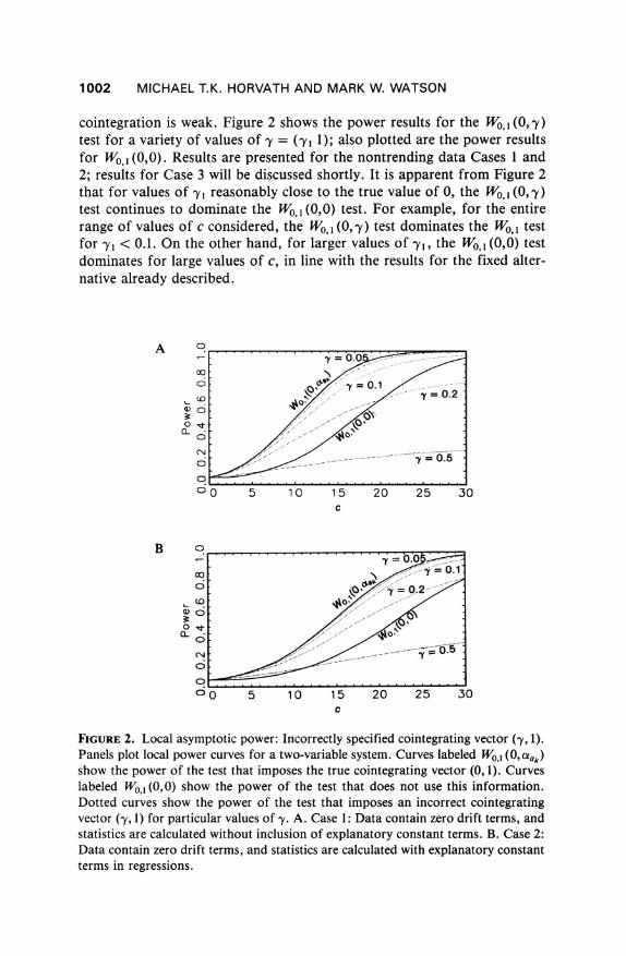
cointegration is weak. Figure 2 shows the power results for the Wo, 1 (0, 'y) test for a variety of values of -y = (-yj 1); also plotted are the power results for W0, 1 (0,0). Results are presented for the nontrending data Cases 1 and 2; results for Case 3 will be discussed shortly. It is apparent from Figure 2 that for values of y I reasonably close to the true value of 0, the WO1 (0, -y) test continues to dominate the W0, 1 (0,0) test. For example, for the entire range of values of c considered, the WO,1 (0, y) test dominates the Wo, 1 test for -yl < 0.1. On the other hand, for larger values of yl, the W0,1 (0,0) test dominates for large values of c, in line with the results for the fixed alternative already described.

A 0

00

.0

?o 5 10 15 20 25 30 c

B 0

0~~~~~~~~~~~0 .

(0

CD.

0

?O 5 10 15 20 25 30 c

FIGURE 2. Local asymptotic power: Incorrectly specified cointegrating vector (-y, 1). Panels plot local power curves for a two-variable system. Curves labeled W0,1 (0, Uidk) show the power of the test that imposes the true cointegrating vector (0, 1). Curves labeled W0,1 (0,0) show the power of the test that does not use this information. Dotted curves show the power of the test that imposes an incorrect cointegrating vector (-y, 1) for particular values of 'y. A. Case 1: Data contain zero drift terms, and statistics are calculated without inclusion of explanatory constant terms. B. Case 2: Data contain zero drift terms, and statistics are calculated with explanatory constant terms in regressions.


The results are quite different in Case 3. These results are not shown because the rejection probability for the test constructed from incorrect values of y I for the WO,1 (O,'y) test are very small for all values of c. The reason for this can be seen from the limiting representation for Wo,I (0, 'y) in Case 3 that was already given. When 'YI *0 the WO,1 (0, y) statistic converges to (sy dB' )' (fJ (s' )2 )-1 (I dB' ), which has a x2 distribution. From Table 1, the 5Gb critical value for the WH0,I (0, 'y) test is 10.18, so that the corresponding rejection probability for the WO,1 (0, 'y) test using the incorrect value of ey is P(X2 > 10.18) = 0.6Gbo.

Arguably, these results for Case 3 have little relevance. After all, when 01 * 0, 'y'Yt will be trending when 'Yi * 0. This behavior would be obvious in a large sample, and so the hypothesis that 'Yt is I(0) could easily be dis- missed. This suggests that the comparison should be made, for example, with 01 or y I local to 0, say 01 = co,/I 12 or 'YI = cYI/T1/2. Because these power functions depend critically on the assumed values of the constant co. and c-,, and because reasonable values of these parameters will differ from application to application, we do not report these functions. Instead, we carry out an experiment for a fixed sample size and Gaussian errors, using values for the parameters in (3.2a) and (3.2b) and values of 'yl that are relevant for a typical application: the analysis of postwar U.S. quarterly data on income and consumption. Letting Yl,t denote the logarithm of per capita consumption and Y2,t denote the logarithm of the consumption/income ratio, then 0l = 0.004, a1 = 0.006, a2 = 0.01 1, cor(1e tE2,t) = 0.21, and T = 175.5 In Fig- ure 3, results are shown for values of y I ranging from 0 to 0.10. For com-

0

00

o /- e ~~~~~~~~= o.o-

0~~~~~~~~~~~~~~l .

00 5 10 15 20 25 30 c

FIGURE 3. Power in the income-consumption system: Incorrectly specified cointegrating vector (y, 1). Panel plots local power curves for a two-variable system with parameters chosen to match the postwar U.S. quarterly data on income and consumption. Notation on curves matches that of Figure 2. See notes for Figure 2 for clarifi- cation.


parison with previous graphs, 62 is written as -c/T, and the power is plotted against c. For this example, the Wo,1 (0, -y) dominates the WO,1 (0,0) statistic for all values of c considered when the error in the postulated cointegrating vector is 5%Wo or less.

When there is only one cointegrating vector under the alternative, simple univariate tests provide an alternative to the likelihood-based tests. Thus, if the cointegrating vector is assumed to be known, then the error correction term a 'yt can be formed and cointegration tested by employing a standard unit root test. The final task of this section is to compare the VECM likelihood- based test to standard univariate tests.

There are three distinct differences between the multivariate tests considered in this paper and standard univariate unit root tests. These are easily discussed in terms of the bivariate example summarized in (3.1) and (3.2). First, univariate tests concentrate on equation (3.2b) and test the simple null, 62 =

0. Multivariate tests consider the whole system (3.1) and test the composite null, 61 = 62 = 0. This has both positive and negative effects: because 61 = 0 (from (3.2a)), the multivariate tests lose power through an extra degree of freedom. In this sense, the univariate test is more powerful because it is focused in the right direction. On the other hand, the multivariate tests utilize any covariance between el, and 62,t to increase test power. This potential covariance is ignored in the univariate tests. The second difference between the univariate and multivariate tests is that the univariate tests typically use a one-sided alternative (62 < 0), whereas the multivariate tests consider two- sided alternatives. The third major difference is the conditioning set used to estimate 62 in (3.2b). In general, lagged first differences enter equation (3.1), so that both the univariate and multivariate tests must be constructed from regressions "augmented" with lags of the variables. The multivariate tests include lagged values of Ay1,, and AY2,t in the regression; univariate procedures, such as augmented Dickey-Fuller regression, include only lags of AY2,t. Thus, when lags of Ayl,t help predict AY2,1, the error term in the multivariate regression will have a smaller variance than the error term in the univariate regression. When Ayl,t and AY2,t are I(0), as assumed here, this leads to a more efficient estimator of 62 and a more powerful test. (Of course, this final point has force only when it is known that yi,t and AY2,t are I(0).)

This last point is the subject of recent papers by Kremers, Ericsson, and Dolado (1992) and Hansen (1993). These papers carefully document the power gains associated with augmenting standard Dickey-Fuller regressions with additional I(0) regressors and allow us to focus instead on the potential power gains and losses associated with the first two differences in the univariate and multivariate procedures. Specifically, Figure 4 compares the power of the univariate and multivariate tests using the same design discussed earlier, but now for various values of p = cor(Cl,tE2,t). All statistics are computed using demeaned values of the data. Two results stand out from


the figure. First, the power functions of the one-sided Dickey-Fuller t-test and the two-sided test based on the squared t-statistic are nearly identical. This is a reflection of the skewed distribution of the Dickey-Fuller t-statistic. Thus, the two-sided nature of the W statistics has little impact on the power relative to the one-sided univariate test. Second, the relative performance of the W(O, a) statistic depends critically on the value of p2, the squared correlation between e,t and E2,t. When p2 = 0, the power loss in the W(0, a) statistic relative to the univariate test corresponds to a sample size reduction of 10o at 5007o power. This is the loss of power associated with the extra degree of freedom in the multivariate test. However, the power gains from exploiting nonzero values for p are large. For example, when P2 = 0.10, the multivariate and univariate tests have essentially identical power. For larger values of p2, the multivariate dominate the univariate tests. For example, when p2 = 0.50, the power gain corresponds to a sample size increase of over 600o at 50!7 power. The reason for this power gain follows from standard seemingly unrelated regression logic: nonzero values of p2 essentially allow the multivariate procedure to partial out part of the error term in (3.2b) and increase the power of the test.

Of course, the results shown in Figure 4 apply to a design with one cointegrating vector in a bivariate system. In a higher dimensional system with only one cointegrating vector, the power of the multivariate test will fall

0

17T-11q I I '

I 1-M." ' - ,1..8j. ........

12 ?p 0.9p-0.75 p0 -5 p20.25

2

p 0.1 DF2'

0

0~~~~~~~

0 o 5 1 0 1 5 20 25 30 C

FIGURE 4. Local asymptotic power. Panel plots local power curves for a two- variable system where the covariance between the error terms is allowed to be different from zero. Solid curves labeled DF and DF2 show the power of one- and two- sided Dickey-FuIler univariate tests for a unit root. The solid curve labeled p2 = 0 shows the power of the Wald test imposing the correct cointegrating vector when the (squared) correlation between the error terms is zero. Dotted curves show the power of the Wald test for different nonzero levels of the squared correlation in the error terms.


because of the extra degrees of freedom. Univariate tests could still be used in this case, but these tests become difficult to use and interpret when there are multiple cointegrating vectors.

4. STABILITY OF THE FORWARD-SPOT FOREIGN EXCHANGE PREMIUM

In this section, we examine forward and spot exchange rates, focusing on whether the forward-spot premium, defined as the forward exchange rate minus the spot exchange rate (in logarithms), is I(O). The data come from Citicorp Database Services, are sampled weekly for the period January 1975 through December 1989 (for a total of 778 observations), and are adjusted for transactions costs induced by bid-ask spreads and for the 2-day/nonholi- day delivery lag for spot market exchange orders, as described in Bekaert and Hodrick (1993).6 The forward-spot premia for the British pound, Swiss franc, German mark, and Japanese yen, the currencies used in our analysis, are shown in Figure 5.

The tests for cointegration are performed on bivariate systems of forward and spot rates in levels, currency by currency. In each case, the number of lagged first differences in the VECM was determined by step-down testing, beginning with a lag length of 18 and using a 5 Wo test for each lag length (for an analysis of step-down testing in the context of testing for unit roots, see Ng and Perron, 1993). Results for testing for cointegration between forward and spot rates are presented in Table 2. For each currency, we report the test statistic for the case where we impose a = ((1 -1)' (denoted by WO I (0, taak)), the test statistic for the case where u is unspecified (denoted by WO I (0,0)), the cointegrating vector estimated in this case (denoted by &'a"), and the ADF statistic calculated from the forward premium. All statistics are reported for the optimal lag length chosen via the step-down procedure. Con-

TABLE 2. Tests for cointegration between spot and forward exchange rates (weekly data, January 1975 to December 1989)

Currency W0,1 (0, eak) WM1 (0,0) ttau ADF

British pound 10.95 (0.04) 10.97 (0.21) [1 - 1.001 (0.004)] -3.12 (0.03) Swiss franc 12.73 (0.02) 13.67 (0.08) [1 - 0.998 (0.003)] -3.33 (0.02) German mark 23.38 (<0.01) 25.00 (<0.01) [1 - 0.999 (0.002)] -3.58 (<0.01) Japanese yen 15.00 (<0.01) 15.02 (0.05) [1 - 1.001 (0.003)] -2.99 (0.04)

Note: The statistics W0,1 (0, oak) were calculated using uak = (1 -1)'. The numbers in parentheses next to the test statistics are p-values. The estimated cointegrating vector &aU is normalized as (1 t), and the numbers in parentheses are the standard errors for 3 computed under the maintained hypothesis that the data are cointegrated.


~~~~~~~~~~~~~~~U 3 )

00 0)

CO

0)

00

00 )

oo U), ,< , A_ . 'tC'

a,

)CL C~~~~~~~c U) 0 n

LO , LO LO ',LO LO U ' E '' (0 L

0 0 0 0~~U C U) N

ci cE c cE c E c E m~~- CO (0z N

o o 0 0 0 0 0 0 o 0 0 0. 0 0 0 0 6 6 o 0 6 6 6 6


stant terms were included in all regressions, and so the p-values for the Wo0 (0, a,,) statistic are from the Case (3) asymptotic null distribution (equivalently Case (2), because a, = 0). Because nominal exchange rates exhibit some trending behavior over the sample period, the p-values for the WO I (0,0) statistic are reported from the Case (3) asymptotic null distribution.

Looking first at the Wo0,I (0, a,k) column, the null of no cointegration is rejected for all currencies at the 5 % level. The Wo, (0,0) statistics, which can be interpreted as WO I (0, ae) maximized over all values of a!, differ little from the Wo I (0, oak) statistics. Their p-values are much greater, however, because their null distribution must account for the fact that they are maximized versions of WO I (0, Q,ak). The next column shows why the two statistics are so similar: the estimated values of the cointegrating vector are equal to (1 -1), out to two decimal places.7 The final column shows the ADF test statistic applied directly to the forward-spot premium. Like the Wo, 1 (0, a!ak)

statistic, the ADF tests reject the null at the 5% level for all of the currencies. This application clearly shows the power advantage of testing for cointegration using a prespecified value of the cointegrating vector. Using the WO I (0,0) statistic, the null of no cointegration is rejected at the 5Wo level for only two of the four currencies.

5. CONCLUDING REMARKS

In this paper, we have generalized VECM-based tests for cointegration to allow for known cointegrating vectors under both the null and alternative hypotheses. The results presented in Section 3 suggest that the power gains associated with these new methods can be substantial. These power gains were evident in the tests for cointegration involving forward and spot exchange rates. Cointegration was found in all currencies using tests that imposed a cointegrating vector of (1 -1), but the null of cointegration was rejected in only half of the cases when this information was not used. Yet, in these bivariate exchange rate models, the univariate ADF test applied to the forward premium (F, - S,) yielded roughly the same inference as the multivariate VECM-based tests that imposed the cointegrating vector. Argu- ably, a more interesting application of the new procedures will be in larger systems with some known and some unknown cointegrating vectors. As argued in Section 3, the power trade-offs in the multivariate and univariate tests for cointegration are more interesting in higher dimensional systems.

The tests developed here rely on simple methods for eliminating trends in the data -incorporating unrestricted constants in the VECM. In the unit root context, the work by Elliott et al. (1995) suggests that large power gains can be achieved using alternative detrending methods. Hence, one extension of the current research will be a thorough investigation of alternative methods of detrending and their effects on tests for cointegration.


NO TES

1. Formally, the restriction rank (6'aa) = ra should be added to the alternative. Because this constraint is satisfied almost surely by the estimators under the alternative, it can be ignored when constructing the likelihood ratio test statistics.

2. The formulation used here is not as general as that used in Johansen (1992a), who consid- ers a model of the form AYt = fi + fl t + II Yt- + ZpI 4,jZYY_j + (,. Johansen's formulation allows for the possibility of quadratic trends in Yt, which are ruled out in our formulation of d,. For more discussion, see Johansen (1992a).

3. There are many repeated entries in Table 1. For example, as already noted, when rau =

0, the Case (2) and Case (3) critical values are identical. Furthermore, within each case, the critical values are the same for all combinations of rak and rau with rak + rau = n - r0U. In this sit- uation when r,, = 0, these hypotheses all correspond to Ho: LI = 0 in equation (2.2). There are a number of other examples of identical critical values that are not listed here.

4. These power curves were computed using 10,000 replications and T 1,000. 5. These parameter values were calculated using consumption and output from the Citibase

Database Services, spanning the quarters 1947:1 through 1990:4, and are in constant (1987) dol- lar, per capita terms. The consumption series is the sum of consumption expenditures on non- durables and services. The output series corresponds to gross, private sector, nonresidential, and domestic product and is constructed as gross domestic product minus farm, nonfarm housing, and government production.

6. We thank Robert Hodrick for making the data available to us. 7. Evans and Lewis (1992) using monthly data over the 1975-1989 period also found esti-

mates of cointegrating vectors very close to (1 -1). While their estimated standard errors suggest that the cointegrating vectors may be different from (I -1), Evans and Lewis argued that this arises from large outliers or "regime shifts" that are evident in the data (see Figure 5). Recent work on robust estimation of cointegrating vectors reported in Phillips (1993) suggests potential efficiency gains for data sets such as the one examined here. Further work is required to determine how the presence of outliers affects the cointegration tests, discussed here.

REFERENCES

Ahn, S.K. & G.C. Reinsel (1990) Estimation for partially nonstationary autoregressive models. Journal of the American Statistical Association 85, 813-823.

Anderson, T.W. (1951) Estimating linear restrictions on regression coefficients for multivariate normal distributions. Annals of Mathematical Statistics 22, 327-351.

Bekaert, G. & R.J. Hodrick (1993) On biases in the measurement of foreign exchange risk pre- miums. Journal of International Money and Finance 12(2), 115-138.

Bobkowsky, M.J. (1983) Hypothesis Testing in Nonstationary Time Series. Ph.D. Thesis, Depart- ment of Statistics, University of Wisconsin.

Brillinger, D.R. (1980) Time Series, Data Analysis and Theory, expanded ed. San Francisco: Holden-Day.

Cavanagh, C.L. (1985) Roots Local to Unity. Manuscript, Department of Economics, Harvard University.

Chan, N.H. (1988) On parameter inference for nearly nonstationary time series. Journal of the American Statistical Association 83, 857-862.

Chan, N.H. & C.Z. Wei (1987) Asymptotic inference for nearly nonstationary AR(1) processes. Annals of Statistics 15, 1050-1063.

Chan, N.H. & C.Z. Wei (1988) Limiting distributions of least squares estimates of unstable autoregressive processes. Annals of Statistics 16(1), 367-401.

Davies, R.B. (1977) Hypothesis testing when a parameter is present only under the alternative. Biometrika 64, 247-254.


Davies, R.B. (1987) Hypothesis testing when a parameter is present only under the alternative. Biometrika 74, 33-43.

Elliott, G. (1993) Efficient Tests for a Unit Root When the Initial Observation Is Drawn from Its Unconditional Distribution. Manuscript, Harvard University.

Elliott, G., T.J. Rothenberg, & J.H. Stock (1995) Efficient tests of an autoregressive unit root. Econometrica, forthcoming.

Engle, R.F. & C.W.J. Granger (1987) Cointegration and error correction: Representation, estimation, and testing. Econometrica 55, 251-276. Reprinted in R.F. Engle & C.W.J. Granger (eds.), Long-Run Economic Relations: Readings in Cointegration. New York: Oxford Uni- versity Press, 1991.

Evans, M.D.D. & K.K. Lewis (1992) Are Foreign Exchange Rates Subject to Permanent Shocks. Manuscript, University of Pennsylvania.

Hansen, B.E. (1990) Inference When a Nuisance Parameter Is Not Identified Under the Null Hypothesis. Manuscript, University of Rochester.

Hansen, B.E. (1993) Testing for Unit Roots Using Covariates. Manuscript, University of Rochester.

Horvath, M. & M. Watson (1995) Critical Values for Likelihood Based Tests for Cointegration When Some of the Cointegrating Vectors Are Prespecified. Manuscript, Stanford University.

Johansen, S. (1988) Statistical analysis of cointegrating vectors. Journal of Economic Dynam- ics and Control 12, 231-254. Reprinted in R.F. Engle & C.W.J. Granger (eds.), Long-Run Economic Relations: Readings in Cointegration. New York: Oxford University Press, 1991.

Johansen, S. (1991) Estimation and hypothesis testing of cointegrating vectors in Gaussian vector autoregression models. Econometrica 59, 1551-1580.

Johansen, S. (1992a) Determination of cointegration rank in the presence of a linear trend. Oxford Bulletin of Economics and Statistics 54, 383-397.

Johansen, S. (1992b) The Role of the Constant Term in Cointegration Analysis of Nonstation- ary Variables. Preprint 1, Institute of Mathematical Statistics, University of Copenhagen.

Johansen, S. & K. Juselius (1990) Maximum likelihood estimation and inference on cointegration-With applications to the demand for money. Oxford Bulletin of Economics and Statistics 52(2), 169-210.

Johansen, S. & K. Juselius (1992) Testing structural hypotheses in a multivariate cointegration analysis of the PPP and UIP of UK. Journal of Econometrics 53, 211-244.

Kremers, J.J.M., N.R. Ericsson, & J.J. Dolado (1992) The power of cointegration tests. Oxford Bulletin of Economics and Statistics 54(3), 325-348.

Ng, S. & P. Perron (1993) Unit Root Tests in ARMA Models with Data Dependent Methods for the Selection of the Truncation Lag. Manuscript, University of Montreal.

Osterwald-Lenum, M. (1992) A note with quantiles of the asymptotic distribution of the maximum likelihood cointegration rank test statistics. Oxford Bulletin of Economics and Statis- tics 54, 461-47 1.

Park, J.Y. (1990) Maximum Likelihood Estimation of Simultaneous Cointegrating Models. Manuscript, Institute of Economics, Aarhus University.

Park, J.Y. & P.C.B. Phillips (1988) Statistical inference in regressions with integrated regressors I. Econometric Theory 4, 468-497.

Phillips, P.C.B. (1987) Toward a unified asymptotic theory for autoregression. Biometrika 74, 535-547.

Phillips, P.C.B. (1988) Multiple regression with integrated regressors. Contemporary Mathemat- ics 80, 79-105.

Phillips, P.C.B. (1991) Optimal inference in cointegrated systems. Econometrica 59(2), 283-306. Phillips, P.C.B. (1993) Robust Nonstationary Regression. Manuscript, Cowles Foundation, Yale

University. Phillips, P.C.B. & B.E. Hansen (1990) Statistical inference in instrumental variables regression

with I(1) processes. Review of Economic Studies 57, 99-125.


Phillips, P.C.B. & V. Solo (1992) Asymptotics for linear processes. Annals of Statistics 20, 971-1001.

Sims, C.A., J.H. Stock, & M.W. Watson (1990) Inference in linear time series models with some unit roots. Econometrica 58(1), 113-144.

Stock, J.H. (1991) Confidence intervals of the largest autoregressive root in U.S. macroeconomic time series. Journal of Monetary Economics 28, 435-460.

Tsay, R.S. & G.C. Tiao (1990) Asymptotic properties of multivariate nonstationary processes with applications to autoregressions. Annals of Statistics 18, 220-250.

APPENDIX

Proof of Theorem 1. To prove the theorem, it is useful to introduce two alternative representations for the model. The first is a triangular simultaneous equations model used by Park (1990); the second is Phillips's (1991) triangular moving average representation. The first representation is useful because it allows the test statistic to be written in a particularly simple form; the second representation is useful because it neatly separates the regressors into I(O) and 1(1) components.

We begin by defining some additional notation. First, partition Y, as Y,- (Y, t Y2, Y',t Y4,)', where Y1,, is r,, x 1, Y2,, is rOk X 1, Y3, is rak x 1, and Y4, t is (n - rou - rOk - rak) x 1. Because the cointegration test statistic is invariant to nonsingular transformations on Yt, we set aeOk = [0 Irok 0 0]' and o!ak = [0 0 Irak 0] a

where these matrices are partitioned conformably with Y,. Thus, ca' = Y2, and O!akYt = Y3,t. Without loss of generality, we write a', = [Irou W2 ?3 0W4] and ot, [0 0 0 &I ], which ensures that the columns of a = [ao ? ak au] are linearly independent. Finally, we assume that the true (but unknown) values of 2, w3, and c4 are 0. These normalizations imply that u1 = (Y',t Y2,)' denotes the 1(0) components of Y, and v, = (Y3, Y4,t)' denotes the I(1), noncointegrated components.

Using this notation, the VECM in equation (2.3) can be reparameterized as the simultaneous equations models

AYI,t = 06Yt-, + olzt + Ei,t, (A.1)

AQt = 6a(Hvti) ?+ y'St + e,, (A.2)

where Qt = (Y2, t Y', t Y4, t)', Si = (A Y t Y2,t, Zt)', and

Irak ?

These equations follow from writing the first rou equations in (2.3) as

=,t =1ouU0'uYt-1 + 1,ok,Y2,t-I + 31,akY3,t-I + a1,au(&t Y4,t-i) + AI Zt + EI,t

(A.3)


and the last (n - r0,) equations as

AQ, = 6Q,O0U uyt-1 + 6Q,okY2,t-I + 6Q,aky3,t-1 + 6Q,au(aauY4,t-l) + IQZt + EQ,t.

(A.4)

In equation (A.1), the term 0'Yt-I captures the effect of all of the error correction terms on AY1,,. Because W2, ?3, and 04 are unknown, 0 is unrestricted. To obtain (A.2), equation (A.3) is solved for c4,uYt- as a function of AY1,,, the other error correction terms, Zt, and el,t; this expression is then substituted into (A.4). Thus, for example, et = eQ,, -

6Q,Ou6 1luel,t in (A.2). In terms of reparameterized models (A. 1) and (A.2), the only constraints on the parameters are those imposed by the null hypothesis: Ho: ga = 0.

Equations (A. 1) and (A.2) are useful because, for given &au, the parameters in (A.2) can be efficiently estimated by 2SLS using Ct = (u I, v,_I, Zt)' as instruments. Thus, letting Q = [Q, Q2 ... QT], V-1 = [VO VI ..e VT-1]', S = [SI S2 ... ST], C= [ Cl C2* CT]', e = [el e2 * eT]', S = C(C'C)-1 C'S, andMS = I- S(S'SY1S', the Wald statistic for testing Ho: ba = 0 using a fixed &au is

W(&eau= [vec(AQ'MSV-1 H')]' [(HV', MSV-1 H')-1 09 E-1 ] [vec(AQ'MVL1 H')]

- [vec(e'MsV_l H')]' [(HVI'1 MsV_l H')-1 0) Se I] [vec(e'MV_l H')],

(A.5)

where the second equality holds under Ho. The asymptotic distribution of SUP&a,W(&a0) depends on the behavior of the

regressors and instruments, which is readily deduced from the triangular moving average representation of the model

ut = Du(L)at + yu, (A.6)

Avv = Dv(L)at + Av, (A.7)

where at = E-U2(t, where Au = 0 in Case 1 and ,Av = 0 in Case 1 and Case 2. Because the variables are generated by a finite order VAR, the matrix coefficients in the lag polynomials Du (L) and Dv (L) eventually decay at an exponential rate. Because v, is I(1) and not cointegrated, D,(1) has full row rank. Furthermore, the error term et in (A.2) can be written as et = Dat, and Dv (1)D' has full row rank because only the first differences of Y1,1 enter (A.2).

The theorem now follows from applying standard results from the analysis of integrated regressors to the components W(&a0) (see, e.g., Chan and Wei, 1988; Park and Phillips, 1988; Phillips, 1988; Sims, Stock, and Watson, 1990; Tsay and Tiao, 1990; or the comprehensive summary in Phillips and Solo, 1992). We now consider the theorem's three cases in turn.

Case 1. In this case, puu = 0 and 4, = 0 in (A.6) and (A.7), and it is readily veri- fied that

T-2V1M?V1 = T2V' l V + op(1) (A.8.i)

T-' V'1Mse = T-1 lVIe + op(l), (A.8.ii)

plim(Se) = e-DD' (A.8.iii)


so that

W(&a,) = [vec(T-'e'VV_IH')]'[(T-2HV', V., H')-' 0& (DD')-']

x [vec(T-1e'V IH')] + op(l).

From the partitioned inverse formula,

[vec(T'-e'V I H')]'[(T-2HV'l V1 H')-' 0 (DD')-'] [vec(T-e'V , H')]

= [vec(T-1e'Vj,_,)]'[(T2 Vj1, V,_,)- 0 (DD')'] [vec(T'e'V,,,)]

+ [vec(T-1e'MV V2,-1 &au)]' [(T2?uv&I Mv, V2,_ &1au) 0a (DD')']

x [vec(T-le'Mvi V2, -1 I au)] , (A.9)

where VI,-, denotes the first rak columns of V,1, and V2,_. denotes the remaining n - - rOk - rak columns. Letting DI denote the first rak rows of Dv(1),

[vec(T-1e' Vj,_ )]' [(T-2 V. _I V.,_ )' 09 (DD')- ] [vec(T-1e' V,_ )]

=Trace[(DD')-/2(T-'e'V1, - I)(T-2 V', - V,,,I)-'(T' V, I e)(DD')-'12']

Trace [(DD )-/2 (DI fBdB'D') (DI fBB'D' (DI fBdB'F')

x (DDI)112i]

= (Trace (F dB Inrot) (F ) (Ff F dBinrou )] (A.10)

where B(s) denotes an n x 1 standard Brownian motion process, F, (s) = BI,rak (S)

(the first rak elements of B(s)), and the last equality denotes equality in distribution. As shown in equation (2.7), maximizing the second terms in (A.9) over all values

of ceau yields

Sup [vec(T'le'Mv v2t-,I au)]'[(T 2& ?,-2 MV V2,i_ a!MuV (0 (DD')']

X [vec (vT- I e'Mv V2,,- &au )]

rau

= >Xi(R) (A.11)

where

R = (DD)12[T- e'Mv, V2,,] [T2 V V, MV, V2,- ] -[T-e'Mv V2,_ ](DD)1/2,

(A.12)

Using notation borrowed from Phillips and Hansen (1990), R is readily seen to con- verge to

R > (fF2dBn-rou)(fF2F2) (F2dB nrou ) (A.13)

where F2(s) = F3(s) - yFI (s), with y = [JF3F;] [fF IF']' where F3(s) = Brak+l,n-ro(S). Case (1) of the theorem follows from (A.10) and (A.13).


Case 2. In Case (2), t,u ? 0 but i,u = 0. Letting V_1 = T-' Z v,-,, the proof follows as in Case (1) with (VI - Vl) replacing VJ I in (A.8)-(A.12) and 3(s) replacing B(s) in limiting representations (A. 10) and (A. 13).

Case 3. In Case (3), both /A and a, * 0. However, because E(cakY,) = 0 is assumed in Case 3, the first rak elements of A, = 0. Thus, the first term of the statistic (the analog of (A. 10)) is identical to the corresponding term in Case 2. The last n - ro0 - rOk - rak elements of v, contain a linear trend, and so, appropriately trans- formed, this set of regressors behaves like a single time trend and n - ro0 - rOk -

rak - 1 martingale components. With this modification, the result for Case (3) follows as in Case (2).

Testing for Cointegration When Some of the Cointegrating ...mwatson/papers/Horvath... · TESTING...

Documents

Transcript of Testing for Cointegration When Some of the Cointegrating ...mwatson/papers/Horvath... · TESTING...