Testing Consistency of Two Histograms*

Frank Porter

California Institute of Technology

Lauritsen Laboratory for High Energy Physics

Pasadena, California 91125

March 7, 2008

Abstract

Several approaches to testing the hypothesis that two histograms are drawn

from the same distribution are investigated. We note that single-sample continuous

distribution tests may be adapted to this two-sample grouped data situation. The

difficulty of not having a fully-specified null hypothesis is an important consideration

in the general case, and care is required in estimating probabilities with “toy” Monte

Carlo simulations. The performance of several common tests is compared; no single

test performs best in all situations.

1. Introduction

Sometimes we have two histograms and are faced with the question: “Are they

consistent?” That is, are our two histograms consistent with having been sampled

from the same parent distribution. For example, we might have a kinematic distri-

bution in two similar channels that we think should be consistent, and wish to test

this hypothesis. Each histogram represents a sampling from a multivariate Poisson

distribution. The question is whether the means are bin-by-bin equal between the

two distributions. Or, if we are only interested in “shape”, are the means related

by the same scale factor for all bins? We investigate this question in the context of

frequency statistics.

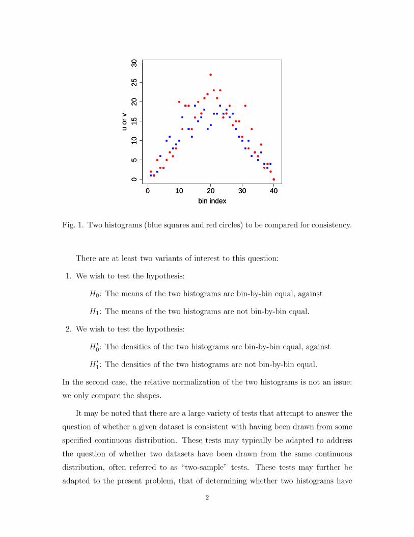
For example, consider Fig. 1. Are the two histograms consistent or can we

conclude that they are drawn from different distributions?

* This work supported in part by the U.S. Department of Energy under grant DE-FG02-

92-ER40701.

1

0 10 20 30 40

05

1015

2025

30

bin index

u or

v

0 10 20 30 40

05

1015

2025

30

bin index

u or

v

Fig. 1. Two histograms (blue squares and red circles) to be compared for consistency.

There are at least two variants of interest to this question:

1. We wish to test the hypothesis:

H0: The means of the two histograms are bin-by-bin equal, against

H1: The means of the two histograms are not bin-by-bin equal.

2. We wish to test the hypothesis:

H ′0: The densities of the two histograms are bin-by-bin equal, against

H ′1: The densities of the two histograms are not bin-by-bin equal.

In the second case, the relative normalization of the two histograms is not an issue:

we only compare the shapes.

It may be noted that there are a large variety of tests that attempt to answer the

question of whether a given dataset is consistent with having been drawn from some

specified continuous distribution. These tests may typically be adapted to address

the question of whether two datasets have been drawn from the same continuous

distribution, often referred to as “two-sample” tests. These tests may further be

adapted to the present problem, that of determining whether two histograms have

2

the same shape. This situation is also referred to as comparing whether two (or

more) rows of a “table” are consistent. The datasets of this form are also referred to

as “grouped data”.

Although we keep the discussion focussed on the comparison of two histograms,

it is worth remarking that many of the observations apply also to other situations,

such as the comparison of a histogram with a model prediction.

2. Notation

We assume that we have formed our two histograms with the same number of

bins, k, with identical bin boundaries. The bin contents of the “first” histogram are

given by realization u of random variable U , and of the second by realization v of

random variable V . Thus, the sampling distributions are:

P (U = u) =

k∏i=1

μui

i

ui!e−μi,

P (V = v) =k∏

i=1

νvi

i

vi!e−νi,

(1)

where the vectors μ and ν are the mean bin contents of the respective histograms.

We define:

Nu ≡k∑

i=1

Ui, total contents of first histogram,

Nv ≡k∑

i=1

Vi, total contents of second histogram,

μT ≡ 〈Nu〉 =k∑

i=1

μi,

νT ≡ 〈Nv〉 =

k∑i=1

νi,

ti ≡ ui + vi, i = 1, . . . , k.

We are interested in the power of a test, at any given confidence level. The power

is the probability that the null hypothesis is rejected when it is false. Of course, the

3

power depends on the true sampling distribution. In other words, the power is one

minus the probability of a Type II error. The confidence level is the probability

that the null hypothesis is accepted, if the null hypothesis is correct. Thus, the

confidence level is one minus the probability of a Type I error. In physics, we usually

don’t specify the confidence level of a test in advance, at least not formally. Instead,

we quote the P -value for our result. This is the probability, under the null hypothesis,

of obtaining a result as “bad” or worse than our observed value. This would be the

probability of a Type I error if our observation were used to define the critical region

of the test.

Note that we are dealing with discrete distributions here, and exact statements of

frequency are problematic, though not impossible. Instead of attempting to construct

exact statements, our treatment of the discreteness will be such as to err on the

“conservative” side. By “conservative”, we mean that we will tend to accept the null

hypothesis with greater than the stated probabitlity. It is important to understand

that this is not always the “conservative” direction, for example it could mislead us

into accepting a model when it should be rejected.

We will drop the distinction between the random variable (upper case symbols

U and V ) and a realization (lower case u and v) in the following, but will point out

where this informality may yield confusion.

The computations in this note are carried out in the framework of the R statistics

package [1].

2.1 Large Statistics Case

If all of the bin contents of both histograms are large, then we may use the

approximation that the bin contents are normally distributed.

Under H0,

〈ui〉 = 〈vi〉 ≡ μi, i = 1, . . . , k.

More properly, it is 〈Ui〉 = μi, etc., but we are permitting ui to stand for the random

variable as well as its realization, as noted above. Let the difference in the contents

4

of bin i between the two histograms be:

Δi ≡ ui − vi,

and let the standard deviation for Δi be denoted σi. Then the sampling distribution

of the difference between the two histograms is:

P (Δ) =1

(2π)k/2

(k∏

i=1

1

σi

)exp

(−1

2

k∑i=1

Δ2i

σ2i

).

This suggests the test statistic:

T =k∑

i=1

Δ2i

σ2i

.

If the σi were known, this would simply be distributed according to the chi-square

distribution with k degrees of freedom. The maximum-likelihood estimator for the

mean of a Poisson is just the sampled number. The mean of the Poisson is also its

variance, and we will use the sampled number also as the estimate of the variance in

the normal approximation.

We suggest the following algorithm for this test:

1. For σ2i form the estimate

σ2i = (ui + vi).

2. Statistic T is thus evaluated according to:

T =k∑

i=1

(ui − vi)2

ui + vi.

If ui = vi = 0 for bin i, the contribution to the sum from that bin is zero.

3. Estimate the P -value according to a chi-square with k degrees of freedom. Note

that this is not an exact result.

If it is desired to only compare shapes, then the suggested algorithm is to scale

both histogram bin contents:

5

1. Let

N = 0.5(Nu + Nv).

Scale u and v according to:

ui → u′i = ui(N/Nu)

vi → v′i = vi(N/Nv).

2. Estimate σ2i with:

σ2i =

(N

Nu

)2

ui +

(N

Nv

)2

vi.

3. Statistic T is thus evaluated according to:

T =

k∑i=1

(ui

Nu− vi

Nv

)2

ui

N2u

+ vi

N2v

.

3. Estimate the P -value according to a chi-square with k − 1 degrees of freedom.

Note that this is not an exact result.

Due to the presence of bins with small bin counts, we might not expect this

method to be especially good for the data in Fig. 1, but we can try it anyway.

Table I gives the results of applying this test, both including the normalization and

only comparing shapes.

Table I. Results of tests for consistency of the two datasets in Fig. 1. The tests below

the χ2 lines are described in Section 3.

Type of test T NDOF P (χ2 > T ) P -value

χ2 Absolute comparison 29.8 40 0.88 0.86

χ2 Shape comparison 24.9 39 0.96 0.95

Likelihood Ratio Shape comparison 25.3 39 0.96 0.96

Kolmogorov-Smirnov Shape comparison 0.043 39 NA 0.61

Bhattacharyya Shape comparison 0.986 39 NA 0.97

Cramer-Von-Mises Shape comparison 0.132 39 NA 0.45

Anderson-Darling Shape comparison 0.849 39 NA 0.45

Likelihood value shape comparison 79 39 NA 0.91

6

In the column labeled “P -value” an attempt is made to compute (by simulation)

a more reliable estimate of the probability, under the null hypothesis, that a value

for T will be as large as that observed. This may be compared with the P (χ2 > T )

column, which is the probability assuming T follows a χ2 distribution with NDOF

degress of freedom.

Note that the absolute comparison yields slightly poorer agreement between the

histograms than the shape comparison. The total number of counts in one dataset

is 492; in the other it is 424. Treating these as samplings from a normal distribution

with variances 492 and 424, we find a difference of 2.2 standard deviations or a two-

tailed P -value of 0.025. This low probability is diluted by the bin-by-bin test. Using a

bin-by-bin test to check whether the totals are consistent is not a powerful approach.

In fact, the two histograms were generated with a 10% difference in expected counts.

The evaluation by simulation of the probability under the null hypothesis is

in fact problematic, since the null hypothesis actually isn’t completely specified.

The problem is the dependence of Poisson probabilities on the absolute numbers of

counts. Probabilities for differences in Poisson counts are not invariant under the

total number of counts. Unfortunately, we don’t know the true mean numbers of

counts in each bin. Thus, we must estimate these means. The procedure adopted

here is to use the maximum likelihood estimators (see below) for the mean numbers,

in the null hypothesis. We’ll have further discussion of this procedure below – it does

not always yield valid results.

In our example, the probabilities estimated according to our simulation and the

probabilities according to a χ2 distribution are close to each other. This suggests

the possibility of using the χ2 probabilities – if we can do this, the problem that we

haven’t completely specified the null hypothesis is avoided. We offer the following

conjecture:

Conjecture: Let T be the test statistic described above, for either the absolute

or the shape comparison, as desired. Let Tc be a possible value of T (perhaps the

critical value to be used in a hypothesis test). Then, for large values of Tc:

P (T < Tc) ≥ P(T < Tc|χ2(T, ndof)

),

where P(T < Tc|χ2(T, ndof)

)is the probability that T < Tc according to a χ2 dis-

7

tribution with ndof degrees of freedom (either k or k − 1, according to which test is

being performed).

We’ll only suggest an approach to a proof, which could presumably also be used

to develop a formal condition for Tc to be “large”. The conjecture also appears to

be true anecdotally, and for interesting values of Tc, noting that it is large values of

Tc that we care most about for an interesting hypothesis test.

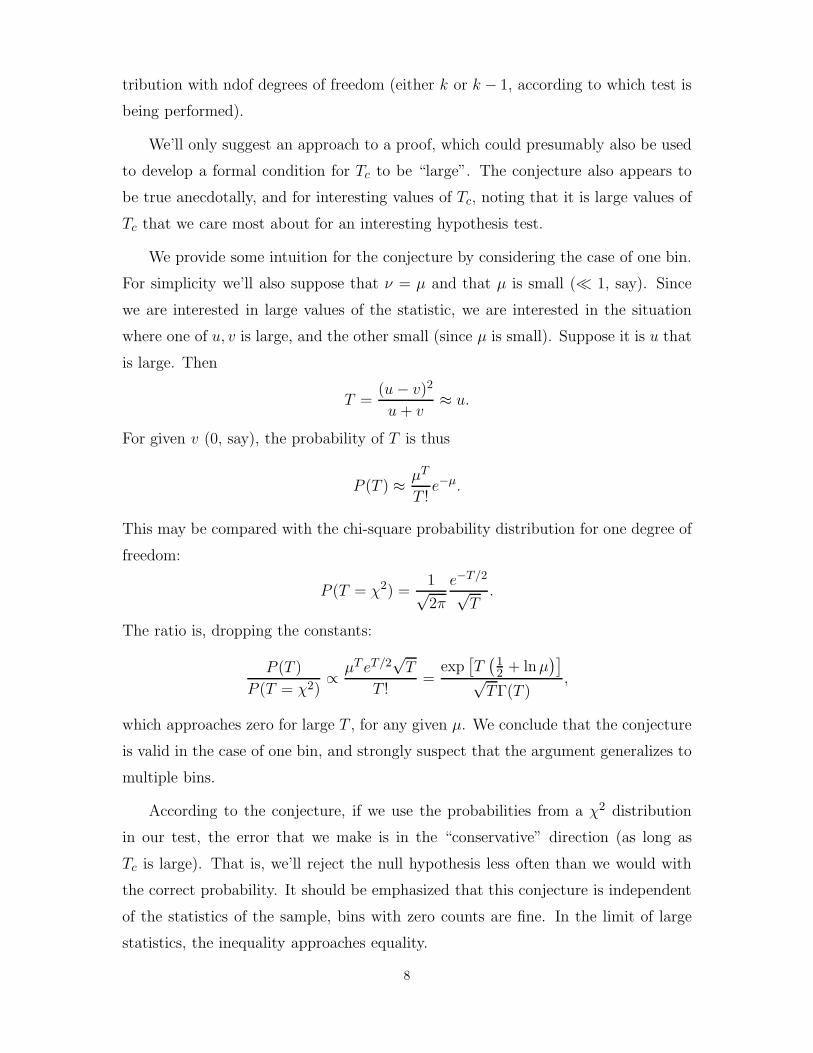
We provide some intuition for the conjecture by considering the case of one bin.

For simplicity we’ll also suppose that ν = μ and that μ is small (� 1, say). Since

we are interested in large values of the statistic, we are interested in the situation

where one of u, v is large, and the other small (since μ is small). Suppose it is u that

is large. Then

T =(u − v)2

u + v≈ u.

For given v (0, say), the probability of T is thus

P (T ) ≈ μT

T !e−μ.

This may be compared with the chi-square probability distribution for one degree of

freedom:

P (T = χ2) =1√2π

e−T/2

√T

.

The ratio is, dropping the constants:

P (T )

P (T = χ2)∝ μT eT/2

√T

T !=

exp[T(

12 + lnμ

)]√

TΓ(T ),

which approaches zero for large T , for any given μ. We conclude that the conjecture

is valid in the case of one bin, and strongly suspect that the argument generalizes to

multiple bins.

According to the conjecture, if we use the probabilities from a χ2 distribution

in our test, the error that we make is in the “conservative” direction (as long as

Tc is large). That is, we’ll reject the null hypothesis less often than we would with

the correct probability. It should be emphasized that this conjecture is independent

of the statistics of the sample, bins with zero counts are fine. In the limit of large

statistics, the inequality approaches equality.

8

Lest we conclude that it is acceptable to just use this great simplification in all

situations, we hasten to point out that it isn’t as nice as it sounds. The problem

is that, in low statistics situations, the power of the test according to this approach

can be dismal. That is, we might not reject the null hypothesis in situations where

it is obviously implausible.

We may illustrate these considerations with some simple examples, see Fig. 2.

The plot for high statistics on the left shows excellent agreement between the actual

distribution and the χ2 distribution. The lower statistics plots in the middle and

right, for two different models, show that the chi-square approximation is very con-

servative in general. Thus, using the chi-square probability lacks power in this case,

and is not a recommended approximation.

60 80 100 120 140Tc

60 80 100 120 14060 80 100 120 140

0.0

0.2

0.4

0.6

0.8

1.0

Tc

Pro

babi

lity(

T<Tc)

60 80 100 120 140

0.0

0.2

0.4

0.6

0.8

1.0

60 80 100 120 140Tc

60 80 100 120 140

(a) (b) (c)

Fig. 2. Comparison of the actual (cumulative) probability distribution for T with the

chi-square distribution. The solid blue curves show the actual distributions, and the

dashed red curves the chi-square distributions. All plots are for 100 bin histograms.

(a) Each bin has mean 100. (b) Each bin has mean 1. (c) Bin j has mean 30/j.

3. General Case

If the bin contents are not necessarily large, then the normal approximation may

not be good enough. There are various approaches we could take in this case. We’ll

discuss and compare several possibilities.

9

3.1 Combining Bins

A simple approach is to combine bins until the normal approximation is good

enough. In many cases this doesn’t lose too much statistical power. It may be

necessary to check with simulations that probability statements are valid. Figure 3

shows the results of this approach on the data in Figure 1, as a function of the

minimum number of events per bin. The comparison being made is for the shapes.

The algorithm is to combine corresponding bins in both histograms until both have

at least “minBin” counts in each bin.

0 10 30 50

010

30

minBin

T or

num

ber o

f bin

s ++++++++++++++++

++++++++++++++++++++++++++++++++++

0 10 30 50

010

30

minBin0 10 30 50

0.0

0.4

0.8

minBin

Prob

abili

ty

+++++++++++++++++++

++++++++++

+++++++

++++

+++++

+++++

0 10 30 50

0.0

0.4

0.8

minBin

Fig. 3. Left: The blue dots show the value of the test statistic T , and the red pluses

shows the number of histogram bins for the data in Fig. 1, as a function of the

minimum number of counts per histogram bin. Right: The P -value for consistency

of the two datasets in Fig. 1. The red pluses show the probability for a chi-square

distribution, and the blue circles show the probability for the actual distribution,

with an estimated null hypothesis.

3.2 Testing for Equal Normalization

An alternative is to work with the Poisson distributions. Let us separate the

problem of the shape from the problem of the overall normalization. In the case of

testing equality of overall normization, there is a well-motivated choice for the test

statistic, even for low statistics.

To test the normalization, we simply compare totals over all bins between the

10

two histograms. Our distribution is

P (Nu, Nv) =μNu

T νNv

T

Nu!Nv!e−(μT +νT ).

The null hypothesis is H0 : μT = νT , to be tested against alternative H1 : μT �= νT .

We are thus interested in the difference between the two means; the sum is effectively

a nuisance parameter. That is, we are interested in

P (Nv|Nu + Nv = N) =P (N |Nv)P (Nv)

P (N)

=μN−Nv

T e−μT

(N − Nv)!

νNv

T e−νT

Nv!

/(μT + νT )Ne−(μT +νT )

N !

=

(N

Nv

)(νT

μT + νT

)Nv(

μT

μT + νT

)N−Nv

.

This probability now permits us to construct a uniformly most powerful test of

our hypothesis (Ref. 2). Note that it is simply a binomial distribution, for given

N . The uniformly most powerful property holds independently of N , although the

probabilities cannot be computed without N .

The null hypothesis corresponds to μT = νT , that is:

P (Nv|Nu + Nv = N) =

(N

Nv

)(1

2

)N

.

For our example, with N = 916 and Nv = 424, the P -value is 0.027, assuming a

two-tailed probability is desired. This may be compared with our earlier estimate

of 0.025 in the normal approximation. Note that for our binomial calculation we

have “conservatively” included the endpoints (424 and 492). If we try to mimic

more closely the normal estimate by subtracting one-half the probability at the

endpoints, we obtain 0.025, essentially the normal number we found earlier. The

dbinom function Ref. 3 in the R package has been used for this computation.

11

3.3 Shape Comparison Statistics

There are many different possible statistics for comparing the shapes of the

histograms. We investigate several choices. Table I summarizes the result of each of

these tests applied to the example in Fig. 1. We list the statistics here, and discuss

performance in the following sections.

3.3.1 Chi-square test for shape

Even though we don’t expect it to follow a χ2 distribution, we may evaluate the

test statistic:

χ2 =

k∑i=1

(ui

Nu− vi

Nv

)2

ui

N2u

+ vi

N2v

.

If ui = vi = 0, the contribution to the sum from that bin is zero. We have already

discussed application of this statistic to the example of Fig. 1.

3.3.2 Geometric test for shape

Another test statistic we could try may be motivated from a geometric perspec-

tive. We consider the bin contents of a histogram to define a vector in a k-dimensional

space. If two such vectors are drawn from the same distribution (the null hypothe-

sis), then they will tend to point in the same direction (we are not interested in the

lengths of the vectors here). Thus, if we represent each histogram as a unit vector

with components:

{u1/Nu, . . . , uk/Nu}, and {v1/Nv, . . . , vk/Nv},

we may form the test statistic:

TBDM =

√u

Nu· v

Nv=

(k∑

i=1

uivi

NuNv

)1/2

.

This is known as the “Bhattacharyya distance measure”. We’ll refer to it as the

“BDM” statistic for short. We assume that neither histogram is empty for this

statistic. All vectors lie in the positive direction in all coordniates, so there is no

issue with taking the square root.

12

It may be noticed that this statistic is related to the χ2 statistic – the uNu

· vNv

dot product is close to the cross term in the χ2 expression.

We apply this formalism to the example in Fig. 1. The resulting terms in the

sum over bins are shown in Fig. 4. The sum over bins gives 0.986 (See Table I for

a summary). According to our estimated distribution of this statistic under the null

hypothesis, this gives a P -value of 0.97, similar to the χ2 test result.

0 10 20 30 40

0.00

0.01

0.02

0.03

0.04

0.05

Bin index

BD

M p

er b

in

BDM statistic

Fre

quen

cy

0.95 0.96 0.97 0.98 0.99

050

0010

000

1500

0

Fig. 4. Left: Bin-by-bin contributions to the geometric (“BDM”) test statistic for

the example of Fig. 1. Right: Estimated distribution of the BDM statistic for the

null hypothesis in the example of Fig. 1.

3.3.3 Kolmogorov-Smirnov test

Another approach to a shape test may be based on the Kolmogorov-Smirnov

(KS) idea. Recall that the idea of the KS test is to estimate the maximum differ-

ence between observed and predicted cumulative distribution functions (CDFs) and

compare with expectations. We may adapt this idea to the present case. It should

be remarked that if we have the actual data points from which the histograms are

derived, then we may use the Kolmogorov-Smirnov (“KS”) procedure directly on

those points. This would incorporate additional information and yield a potentially

more powerful test. However, if the bin widths are small compared with possible

structure it may be expected to not make much difference.

13

We modify the KS statistic to apply to comparison of histograms as follows.

We assume that neither histogram is empty. Form the “cumulative distribution

histograms” according to:

uci =i∑

j=1

uj/Nu

vci =

i∑j=1

vj/Nv.

Then compute the test statistic:

TKS = maxi

|uci − vci|.

Test statistics may also be formed for one-tail tests, but we consider only the two-tail

test here.

We apply this formalism to the example in Fig. 1. The bin-by-bin distances are

shown in Fig. 5. The maximum over bins gives 0.043 (See Table I for a summary).

According to our estimated distribution of this statistic under the null hypothesis,

this gives a P -value of 0.61, somewhat smaller than for the χ2 test result, but still

indicating consistency of the two histograms. Note that the KS test tends to empha-

size the region near the peak of the distribution, that is the region where the largest

fluctuations are expected in Poisson statistics.

0 10 20 30−0.

100.

000.

10

Bin index

KS d

ista

nce

KS statistic

Freq

uenc

y

0.02 0.08 0.14

010

0025

00

Fig. 5. Left: Bin-by-bin distances for the Kolmogorov-Smirnov test statistic for

the example of Fig. 1. Right: Estimated distribution of the Kolmogorov-Smirnov

distance for the null hypothesis in the example of Fig. 1.

14

3.3.4 Cramer-von-Mises test

Somewhat similar to the Kolmogorov-Smirnov test is the Cramer-von-Mises

(CVM) test. The idea in this test is to add up the squared differences between

the cumulative distributions being compared. Again, this test is usually thought of

as a test to compare an observed distribution with a presumed parent continuous

probability distribution. However, the algorithm can be adapted to the two-sample

comparison, and to the case of comparing two histograms.

The test statistic for comparing the two samples x1, x2, . . . , xN and y1, y2, . . . , yM

is [4]:

T =NM

(N + M)2

⎧⎨⎩

N∑i=1

[Ex(xi) − Ey(xi)]2 +

M∑j=1

[Ex(yj) − Ey(yj)]2

⎫⎬⎭ ,

where Ex is the empirical cumulative distribution for sampling x. That is, Ex(x) =

n/N if n of the sampled xi are less than or equal to x.

We adapt this for the present application of comparing histograms with bin

contents u1, u2, . . . , uk and v1, v2, . . . , vk with identical bin boundaries: Let z be a

point in bin i, and define the empirical cumulative distribution function for histogram

u as:

Eu(z) =

i∑j=1

ui/Nu.

Then the test statistic is:

TCVM =NuNv

(Nu + Nv)2

k∑j=1

(uj + vj) [Eu(zj) − Ev(zj)]2 .

We apply this formalism to the example in Fig. 1, finding TCVM = 0.132. The

resulting estimated distribution under the null hypothesis is shown in Fig. 6. Ac-

cording to our estimated distribution of this statistic under the null hypothesis, this

gives a P -value of 0.45 (See Table I for a summary), somewhat smaller than the χ2

test result.

15

CVM statistic

Fre

quen

cy

0.0 0.5 1.0 1.5

010

0020

0030

0040

00

AD statistic

Fre

quen

cy

0 2 4 6

010

0020

0030

0040

00Fig. 6. Estimated distributions of the test statistic for the null hypothesis in the ex-

ample of Fig. 1 Left: The Cramer-von-Mises statistic. Right: The Anderson-Darling

statistic.

3.3.5 Anderson-Darling test for shape

The Anderson-Darling test is another variant on the theme of non-parametric

comparison of cumulative distributions. It is similar to the Cramer-von-Mises statis-

tic, but is designed to be sensitive to the tails of the CDF. The original statistic was,

once again, designed to compare a dataset drawn from a continuous distribution,

with CDF F0(x) under the null hypothesis:

A2m = m

∫ ∞

−∞[Fm(x) − F0(x)]2

F0(x) [1 − F0(x)]dF0(x),

where Fm(x) is the empirical CDF of dataset x1, . . . xm. Scholz and Stephens [5]

provide a form of this statistic for a k-sample test on grouped data (e.g., as might

be used to compare k histograms). Based on the result expressed in their Eq. 6, the

expression of interest to us for two histograms is:

TAD =1

Nu + Nv

kmax−1∑j=kmin

tjΣj (Nu + Nv − Σj)

{[(Nu + Nv)Σuj − NuΣj ]

2 /Nu

+ [(Nu + Nv)Σvj − NvΣj ]2 /Nv

},

16

where kmin is the first bin where either histogram has non-zero counts, kmax is the

number of bins counting up the the last bin where either histogram has non-zero

counts, and

Σuj ≡j∑

i=1

ui,

Σvj ≡j∑

i=1

vi, and

Σj ≡j∑

i=1

ti = Σuj + Σvj .

We apply this formalism to the example in Fig. 1. The resulting estimated

distribution under the null hypothesis is shown in Fig. 6. The sum over bins gives

0.849 (See Table I for a summary). According to our estimated distribution of this

statistic under the null hypothesis, this gives a P -value of 0.45, somewhat smaller

than the χ2 test result, but similar with the CVM result.

3.3.6 Likelihood ratio test for shape

We may base a test whether the histograms are sampled from the same shape

distribution on the same binomial idea as we used for the normalization test. In this

case, however, there is a binomial associated with each bin of the histogram. We

start with the null hypothesis, that the two histograms are sampled from the joint

distribution:

P (u, v) =

k∏i=1

μui

i

ui!e−μi

νvi

i

vi!e−νi,

where νi = aμi for i = 1, 2, . . . , k. That is, the “shapes” of the two histograms are

the same, although the total contents may differ.

With ti = ui + vi, and fixing the ti at the observed values, we have the multi-

binomial form:

P (v|u + v = t) =k∏

i=1

(ti

vi

)(νi

νi + μi

)vi(

μi

νi + μi

)ti−vi

.

The null hypothesis is that νi = aμi for all values of i. We would like to test this,

but there are now two complications:

17

1. The value of “a” is not specified;

2. We still have a multivariate distribution.

For a, we will substitute an estimate from the data, namely the maximum like-

lihood estimator:

a =Nv

Nu.

Note that this estimate is a random variable; its use will reduce the effective number

of degrees of freedom by one.

We propose to use a likelihood ratio statistic to reduce the problem to a single

variable. This will be the likelihood under the null hypothesis (with a given by its

maximum likelihood estimator), divided by the maximum of the likelihood under the

alternative hypothesis. Thus, we form the ratio:

λ =maxH0

L(a|v; u + v = t)

maxH1L({ai ≡ νi/μi}|v; u + v = t)

=

k∏i=1

(a

1+a

)vi ( 11+a

)ti−vi(ai

1+ai

)vi(

11+ai

)ti−vi.

The maximum likelihood estimator, under H1, for ai is just

ai = vi/ui.

Thus, we rewrite our test statistic according to:

λ =k∏

i=1

(1 + vi/ui

1 + Nv/Nu

)ti(

Nv

Nu

ui

vi

)vi

.

In practice, we’ll work with

−2 ln λ = −2

k∑i=1

[ti ln

(1 + vi/ui

1 + Nv/Nu

)+ vi ln

(Nv

Nu

ui

vi

)].

Before attempting to apply this, we investigate how to handle zero bin contents.

It is possible that ui = vi = 0 for some bin. In this case, P (vi|ui + vi = ti) = 1,

18

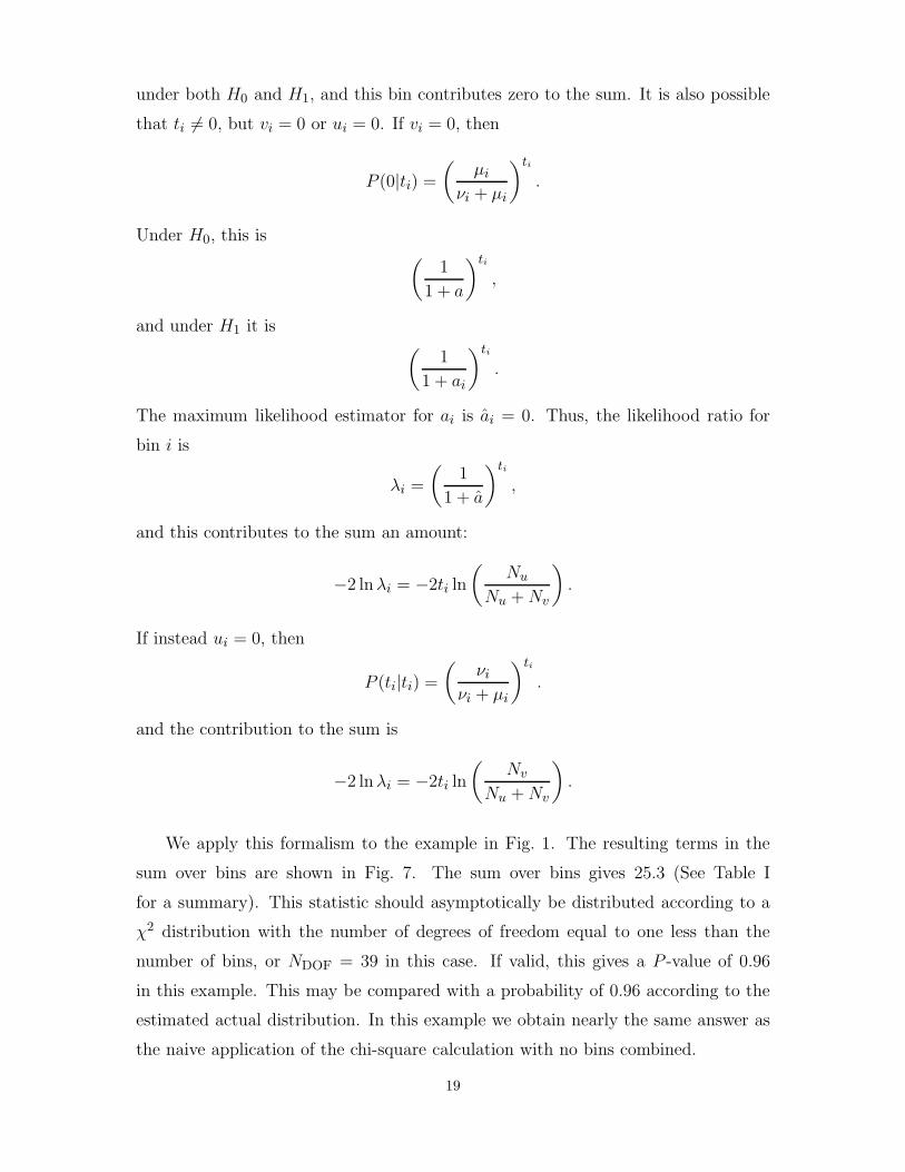
under both H0 and H1, and this bin contributes zero to the sum. It is also possible

that ti �= 0, but vi = 0 or ui = 0. If vi = 0, then

P (0|ti) =

(μi

νi + μi

)ti

.

Under H0, this is (1

1 + a

)ti

,

and under H1 it is (1

1 + ai

)ti

.

The maximum likelihood estimator for ai is ai = 0. Thus, the likelihood ratio for

bin i is

λi =

(1

1 + a

)ti

,

and this contributes to the sum an amount:

−2 lnλi = −2ti ln

(Nu

Nu + Nv

).

If instead ui = 0, then

P (ti|ti) =

(νi

νi + μi

)ti

.

and the contribution to the sum is

−2 lnλi = −2ti ln

(Nv

Nu + Nv

).

We apply this formalism to the example in Fig. 1. The resulting terms in the

sum over bins are shown in Fig. 7. The sum over bins gives 25.3 (See Table I

for a summary). This statistic should asymptotically be distributed according to a

χ2 distribution with the number of degrees of freedom equal to one less than the

number of bins, or NDOF = 39 in this case. If valid, this gives a P -value of 0.96

in this example. This may be compared with a probability of 0.96 according to the

estimated actual distribution. In this example we obtain nearly the same answer as

the naive application of the chi-square calculation with no bins combined.

19

0 10 20 30

01

23

4

Bin index

−2l

n(la

mbd

a)

0 10 20 30

01

23

4

Fig. 7. Value of −2 lnλi or χ2i as a function of histogram bin in the comparison of

the two distributions of Fig. 1. Blue circles are −2 ln λi; red squares are χ2i .

We may see that this close agreement is a result of nearly bin-by-bin equality of

the two statistics, see Fig. 7. To investigate when this might hold more generally, we

compare the values of −2 ln λi and χ2i as a function of ui and vi, Fig. 8. We observe

that the two statistics agree when ui = vi with increasing difference away from that

point. This observation is readily verified analytically. This agreement holds even

for low statistics. However, we shouldn’t conclude that the chi-square approximation

may be used for low statistics – fluctuations away from equal numbers lead to quite

different results when we get into the tails at low statistics. Our example doesn’t

really sample these tails.

The precise value of the probability should not be taken too seriously, except

to conclude that the two distributions are consistent according to these tests. For

example, when we combine bins to improve expected χ2 behavior, we see fairly large

fluctuations in the probability estimate just due to the re-binning (Fig. 3).

20

0

2

4

6

8

10

12

14

16

0 2 4 6 8 10v

T

chisq, u=0-2lnL, u=0chisq, u=5-2lnL, u=5chisq, u=10-2lnL, u=10

Fig. 8. Value of −2 ln λi or χ2i as a function of ui and vi bin contents. This plot

assumes Nu = Nv. The i subscript is dropped, with the understanding that this

comparison is for a single bin.

3.3.7 Likelihood value test for shape

An often-used but controversial goodness-of-fit statistic is the value of the like-

lihood at its maximum value under the null hypothesis. It can be demonstrated

that this statistic carries little or no information in some situations. However, in the

limit of large statistics it is essentially the chi-square statistic, so there are known

situations were it is a plausible statistic to use. We thus look at it here.

Using the results in the previous section, the test statistic is:

T = − lnL = −k∑

i=1

[ln

(ti

vi

)+ ti ln

Nu

Nu + Nv+ vi ln

Nv

Nu

].

If either Nu = 0 or Nv = 0, then T = 0.

We apply this formalism to the example in Fig. 1. The resulting estimated

distribution under the null hypothesis is shown in Fig. 9. The sum over bins gives

90 (See Table I for a summary). According to our estimated distribution of this

statistic under the null hypothesis, this gives a P -value of 0.29, similar to the χ2 test

result. The fact that it is similar may be expected from the fact that our example is

reasonably well-approximated by the large statistics limit.

21

ln Likelihood

Fre

quen

cy

75 80 85 90 95 100 105

050

010

0015

00

Fig. 9. Estimated distribution of the lnL test statistic for the null hypothesis in the

example of Fig. 1.

There are many other possible tests that could be considered, for example,

schemes that “partition” the χ2 to select sensitivity to different characteristics [6].

3.4 Distributions Under the Null Hypothesis

For the situation where the asymptotic distribution may not be good enough,

we would like to know the probability distribution of our test statistic under the null

hypothesis. However, we encounter a difficulty: our null hypothesis is not completely

specified! The problem is that the distribution depends on the values of νi = aμi.

Our null hypothesis only says νi = aμi, but says nothing about what μi might be.

Note that it also doesn’t specify a, but we have already discussed that complication,

which appears manageable (although in extreme situations one might need to check

for dependence on a).

We turn once again to the data to make an estimate for μi, to be used in esti-

mating the distribution of our test statistics. The straightforward approach is to use

the maximum likelihood parameter estimators (under H0):

μi =1

1 + a(ui + vi),

νi =a

1 + a(ui + vi),

22

where a = Nv/Nu. The data is then repeatedly simulated using these values for

the parameters of the sampling distribution. For each simulation, a value of the

test statistic is obtained. The distribution so obtained is then an estimate of the

distribution of the test statistic under the null hypothesis, and P -values may be

computed from this. Variations in the estimates for μi and a may be used to check

robustness of the probability estimates obtained in this way.

We have just described the approach that was used to compute the estimated

probabilities for the example of Fig. 1. The bin contents in this case are reasonably

large, and this approach works well enough for this case.

Unfortunately, this approach does very poorly in the low-statistics realm. We

consider a simple test case: Suppose our data is sampled from a flat distribution

with a mean of 1 count in each of 100 bins. We test how well our estimated null

hypothesis works for any given test statistic, T , as follows:

1. Generate a pair of histograms according to the distribution just described.

(a) Compute T for this pair of histograms.

(b) Given the pair of histograms, compute the estimated null hypothesis accord-

ing to the spcified prescription above.

(c) Generate many pairs of histograms according to the estimated null hypothesis

in order to obtain an estimated distribution for T .

(d) Using the estimated distribution for T , determine the estimated P -value for

the value of T found in step 1a.

2. Repeat step 1 many times and make a histogram of the estimated P -values.

Note that this histogram should be uniform if the estimated P -values are good

estimates.

23

The distributions of the estimated probabilities for the seven test statistics under

the null hypothesis are shown in the second column of Fig. 10. If the null hypothesis

were to be rejected at the estimated 0.01 probability, this algortihm would actually

reject H0 19% of the time for the χ2 statistic, 16% of the time for the BDM statistic,

24% of the time for the lnλ statistic, and 29% of the time for the L statistics, all

unacceptably larger than the desired 1%. The KS, CVM, and AD statistics are all

consistent with the desired 1%. For comparison, the first column of Fig. 10 shows

the distribution for a “large statistics” case, where sampling is from histograms with

a mean of 100 counts in each bin. We find that all test statistics display the desired

flat distribution in this case. Table II summarizes these results.

Table II. Probability that the null hypothesis will be rejected with a cut at 1% on

the estimated distribution (see text). H0 is estimated with the bin-by-bin algorithm

in the first two columns, by the uniform histogram algorithm in the third column,

and with a Gaussian kernel estimation in the fourth column.

Test statistic Probability (%) Probability (%) Probability (%) Probability (%)

Bin mean = 100 1 1 (uniform) 1 (kernel)

H0 estimate bin-by-bin bin-by-bin uniform kernel

χ2 0.97 ± 0.24 18.5 ± 1.0 1.2 ± 0.3 1.33 ± 0.28

BDM 0.91 ± 0.23 16.4 ± 0.9 0.30 ± 0.14 0.79 ± 0.22

KS 1.12 ± 0.26 0.97 ± 0.24 1.0 ± 0.2 1.21 ± 0.27

CVM 1.09 ± 0.26 0.85 ± 0.23 0.8 ± 0.2 1.27 ± 0.28

AD 1.15 ± 0.26 0.85 ± 0.23 1.0 ± 0.2 1.39 ± 0.29

ln λ 0.97 ± 0.24 24.2 ± 1.1 1.5 ± 0.3 2.0 ± 0.34

lnL 0.97 ± 0.24 28.5 ± 1.1 0.0 ± 0.0 0.061 ± 0.061

24

05

1015

2025

05

1015

2025

300

510

1520

250

510

15

20

25

05

1015

2025

300

510

1520

2530

Estimated probability0.0 0.2 0.4 0.6 0.8 1.0

01

02

03

0

Fre

quen

cy0

510

1520

25

05

015

025

0

Fre

quen

cy0

510

1520

25

05

010

020

0

Fre

quen

cy0

510

1520

25

05

1015

2025

30

Fre

quen

cy0

510

15

20

25

05

101

52

02

53

0

Fre

quen

cy0

510

1520

2530

05

1015

2025

30

Fre

quen

cy0

510

1520

25

010

020

030

040

0

Estimated probability

Fre

quen

cy

0.0 0.2 0.4 0.6 0.8 1.0

05

1015

2025

30

Estimated probability0.0 0.2 0.4 0.6 0.8 1.0

010

020

030

040

0

2χ

BDM

KS

CVM

AD

ln

ln

λ

L

05

1015

2025

300

510

1520

2530

05

1015

2025

05

1015

2025

300

510

1520

2530

05

1015

2025

30

Estimated probability0.0 0.2 0.4 0.6 0.8 1.0

010

2030

Fig. 10. See caption on next page25

Fig. 10. (Figure on previous page) Distribution of the estimated probability that

the test statistic is worse than that observed, for seven different test statistics. The

data are generated according to the null hypothesis, consisting of 100 bin histograms

with a mean of 100 counts (left column) or one count (other columns). The first

and second columns are for an estimated H0 computed as the weighted bin-by-bin

average. The third column is for an estimated H0 where each bin is the average of

the total contents of both histograms, divided by the number of bins. The rightmost

column is for an estimated H0 estimated with a Gaussian kernel estimator using the

contents of both histograms. The χ2 is computed without combining bins.

It may be noted that the issue really is one appearing at low statistics. We

can give some intuition for the observed effect. Consider the likely scenario at low

statistics that some bins will have zero counts in both histograms. In this case our

algorithm for the estimated null hypothesis yields a zero mean for these bins. The

simulation used to determine the probability distribution for the test statistic will

always have zero counts in these bins, that is, there will always be agreement between

the two histograms in these bins. Thus, the simulation will find that values of the

test statistic are more probable than it should.

If we tried the same study with, say, a mean of 100 counts per bin, we would

find that the probability estimates are valid, at least this far into the tails. The left

column of Fig. 10 shows that more sensible behavior is achieved with larger statistics.

The χ2, ln λ, and lnL statistics perform essentially identically at high statistics, as

expected, since in the normal approximation they are equivalent.

The AD, CVM, and KS tests are more robust under our estimates of H0 than the

others, as they tend to emphasize the largest differences and are not so sensitive to

bins that always agree. For these statistics, we see that our procedure for estimating

H0 does well even for low statistics, although we caution again that we are not

examining the far tails of the distribution.

There are various possible approaches to salvaging the situation in the low statis-

tics regime. Perhaps the simplest is to rely on the typically valid assumption that

the underlying H0 distribution is “smooth”. Then instead of having an unknown

parameter for each bin, we only need to estimate a few parameters to describe the

smooth distribution, and effectively more statistics are available.

26

For example, we may repeat the algorithm for our example of a mean of one

count per bin, but now assuming a smooth background represented by a uniform

distribution. This is cheating a bit, since we perhaps aren’t supposed to know that

this is really what we are sampling from, but we’ll pretend that we looked at the

data and decided that this was plausible. As usual, we would in practice want to try

other possibilities to evaluate systematic effects.

Thus, we estimate:

μi = Nu/k, i = 1, 2, . . . , k

νi = Nv/k, i = 1, 2, . . . , k.

The resulting distributions for the estimated probabilities are shown in the third

column of Fig. 10. These distributions are much more reasonable, at least at the

level of a per cent (1650 sample experiments are generated in each case, and the

estimated P value is estimated for each experiment with 1650 evaluations of the null

hypothesis for that experiment).

It should be remarked that the lnL and, perhaps, to a much lesser extent the

BDM statistic, do not give the desired 1% result, but now err on the “conservative”

side. It may be possible to mitigate this with a different algorithm, but this has not

been investigated. We may expect the power of these statistics to suffer under the

approach taken here.

Since we aren’t supposed to know that our null distribution is uniform, we also

try another approach to get a feeling for whether we can really do a legitimate

analysis. Thus, we try a kernel estimator for the null distribution, using the sum of

the observed histograms as input. In this case, we have chosen a Gaussian kernel,

with a standard deviation of 2. The “density” package in R [1] is used for this. An

example of such a kernel estimated distribution is shown in Fig. 11. The resulting

estimated probability distributions of our test statistics are shown in the rightmost

column of Fig. 10. In general, this works pretty well. The bandwidth was chosen

here to be rather small; a larger bandwidth would presumably improve the results.

27

0 20 40 60 80 1000.00

40.

008

0.01

20.

016

bin

Den

sity

Fig. 11. Sample Gaussian kernel density estimate of the null hypothesis (for sampling

from a true null).

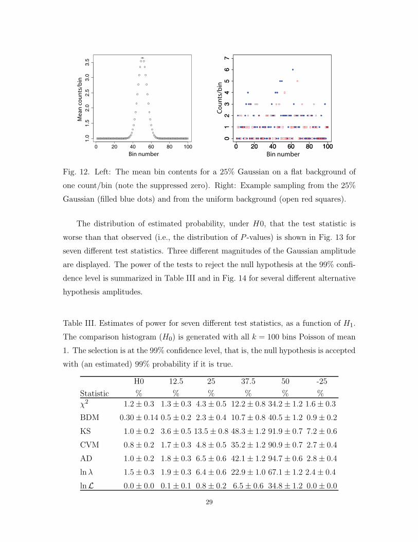
3.5 Comparison of Power of Tests

The power depends on what the alternative hypothesis is. Here, we mostly inves-

tigate adding a Gaussian component on top of a uniform background distribution.

This choice is motivated by the scenario where one distribution appears to show

some peaking structure, while the other does not. We also look briefly at a different

extreme, that of a rapidly varying alternative.

The data for this study are generated as follows: The background (null distri-

bution) has a mean of one event per histogram bin. The Gaussian has a mean of 50

and a standard deviation of 5, in units of bin number. We vary the amplitude of the

Gaussian and count how often the null hypothesis is rejected at the 1% confidence

level. The amplitude is measured in percent, for example a 25% Gaussian has a total

amplitude corresponding to an average of 25% of the total counts in the histogram,

including the (small) tails extending beyond the histogram boundaries. The Gaus-

sian counts are added to the counts from the null distribution. An example is shown

in Fig. 12.

28

0 20 40 60 80 100

1.0

1.5

2.0

2.5

3.0

3.5

Bin number

Mea

n c

ou

nts

/bin

0 20 40 60 80 100

01

23

45

67

0 20 40 60 80 100

01

23

45

67

Bin number

Co

un

ts/b

in

Fig. 12. Left: The mean bin contents for a 25% Gaussian on a flat background of

one count/bin (note the suppressed zero). Right: Example sampling from the 25%

Gaussian (filled blue dots) and from the uniform background (open red squares).

The distribution of estimated probability, under H0, that the test statistic is

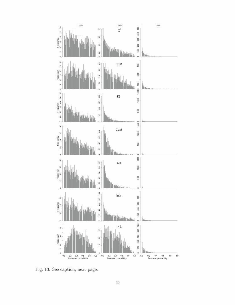
worse than that observed (i.e., the distribution of P -values) is shown in Fig. 13 for

seven different test statistics. Three different magnitudes of the Gaussian amplitude

are displayed. The power of the tests to reject the null hypothesis at the 99% confi-

dence level is summarized in Table III and in Fig. 14 for several different alternative

hypothesis amplitudes.

Table III. Estimates of power for seven different test statistics, as a function of H1.

The comparison histogram (H0) is generated with all k = 100 bins Poisson of mean

1. The selection is at the 99% confidence level, that is, the null hypothesis is accepted

with (an estimated) 99% probability if it is true.

H0 12.5 25 37.5 50 -25

Statistic % % % % % %

χ2 1.2 ± 0.3 1.3 ± 0.3 4.3 ± 0.5 12.2 ± 0.8 34.2 ± 1.2 1.6 ± 0.3

BDM 0.30 ± 0.14 0.5 ± 0.2 2.3 ± 0.4 10.7 ± 0.8 40.5 ± 1.2 0.9 ± 0.2

KS 1.0 ± 0.2 3.6 ± 0.5 13.5 ± 0.8 48.3 ± 1.2 91.9 ± 0.7 7.2 ± 0.6

CVM 0.8 ± 0.2 1.7 ± 0.3 4.8 ± 0.5 35.2 ± 1.2 90.9 ± 0.7 2.7 ± 0.4

AD 1.0 ± 0.2 1.8 ± 0.3 6.5 ± 0.6 42.1 ± 1.2 94.7 ± 0.6 2.8 ± 0.4

ln λ 1.5 ± 0.3 1.9 ± 0.3 6.4 ± 0.6 22.9 ± 1.0 67.1 ± 1.2 2.4 ± 0.4

lnL 0.0 ± 0.0 0.1 ± 0.1 0.8 ± 0.2 6.5 ± 0.6 34.8 ± 1.2 0.0 ± 0.0

29

Fre

quen

cy0

510

1520

2530

01

03

05

07

0

010

020

030

040

050

0

12.5% 25% 50%

2χ

Fre

quen

cy0

510

1520

2530

01

02

03

04

0

010

030

050

0BDM

Fre

quen

cy0

10

20

30

40

50

60

05

010

015

020

0

05

0010

0015

00

KS

Fre

quen

cy0

10

20

30

40

02

04

06

08

0

050

010

0015

00

CVM

05

0010

0015

00

Fre

quen

cy0

10

20

30

40

02

04

06

08

010

0

AD

020

040

060

080

0

Fre

quen

cy0

10

20

30

02

04

06

08

010

0

lnλ

Estimated probability0.0 0.2 0.4 0.6 0.8 1.0

010

020

030

040

050

0

Estimated probability

Fre

quen

cy

0.0 0.2 0.4 0.6 0.8 1.0

05

1020

30

Estimated probability0.0 0.2 0.4 0.6 0.8 1.0

01

02

03

0

lnL

Fig. 13. See caption, next page.

30

Fig. 13. (Figure on previous page) Distribution of estimated probability, under H0,

that the test statistic is worse than that observed, for seven different test statistics.

The data are generated according to a uniform distribution, consisting of 100 bin

histograms with a mean of 1 count, for one histogram, and for the other histogram

with a uniform distribution plus a Gaussian of strength 12.5% (left column), 25%

(middle column), and 50% (right column). The χ2 is computed without combining

bins.

Pow

er (%

)

Gaussian Amplitude (%)

Fig. 14. Summary of power of seven different test statistics, for the alternative

hypothesis with a Gaussian bump. Left: linear vertical scale; Right: logarithmic

vertical scale. [Best viewed in color. At an amplitude of 35%, the ordering, from top

to bottom, of the curves is: KS, AD, CVM, ln λ, χ2, BDM, lnL.]

In Table IV we take a look at the performance of our seven statistics for his-

tograms with large bin contents. It is interesting that in this large-statistics case, for

the χ2 and similar tests, the power to reject a dip is greater than the power to reject

a bump of the same area. This is presumably because the “error estimates” for the

χ2 are based on the square root of the observed counts, and hence give smaller errors

for smaller bin contents. We also observe that the comparative strength of the KS,

CVM, and AD tests versus the χ2, BDM, lnλ, and lnL tests in the small statistics

situation is largely reversed in the large statistics case.

31

Table IV. Estimates of power for seven different test statistics, as a function of H1.

The comparison histogram (H0) is generated with all k = 100 bins Poisson of mean

100. The selection is at the 99% confidence level.

H0 5 -5

Statistic % % %

χ2 0.91 ± 0.23 79.9 ± 1.0 92.1 ± 0.7

BDM 0.97 ± 0.24 80.1 ± 1.0 92.2 ± 0.7

KS 1.03 ± 0.25 77.3 ± 1.0 77.6 ± 1.0

CVM 0.91 ± 0.23 69.0 ± 1.1 62.4 ± 1.2

AD 0.91 ± 0.23 67.5 ± 1.2 57.8 ± 1.2

ln λ 0.91 ± 0.23 79.9 ± 1.0 92.1 ± 0.7

lnL 0.97 ± 0.24 79.9 ± 1.0 91.9 ± 0.7

To get an idea of what happens for a radically different alternative to the null

distribution, we consider sensitivity to sampling from the “sawtooth” distribution as

shown in figure 15. This is to be compared once again to samplings from the uniform

histogram. The results are tabulated in Table V. The “percentage” sawtooth here

refers to the fraction of the null hypothesis mean. That is, a 100% sawtooth on a 1

count/bin background oscillates between a mean of 0 counts/bin and 2 counts/bin.

The period of the sawtooth is always two bins.

0 20 40 60 80 100

0.0

0.5

1.0

1.5

2.0

Bin number

H0

or H

1 m

ean

0 20 40 60 80 100

0.0

0.5

1.0

1.5

2.0

0 20 40 60 80 100

01

23

45

Bin number

Cou

nts/

bin

0 20 40 60 80 100

01

23

45

Fig. 15. Left: The mean bin contents for a 50% sawtooth on a flat background

of one count/bin (blue), compared with the flat background means (red). Right:

Example sampling from the 50% sawtooth (filled blue dots) and from the uniform

background (open red squares).

32

In this example, the χ2 and likelihood ratio tests are the clear winners, with

BDM next. The KS, CVM, and AD tests reject the null hypothesis with the same

probability as for sampling from a true null distribution. This very poor performance

for these tests is readily understood, as these tests are all based on the cumulative

distributions, which average out local oscillations.

Table V. Estimates of power for seven different test statistics, for a “sawtooth”

alternative distribution.

50 100

Statistic % %

χ2 3.7 ± 0.5 47.8 ± 1.2

BDM 1.9 ± 0.3 33.6 ± 1.2

KS 0.85 ± 0.23 1.0 ± 0.2

CVM 0.91 ± 0.23 1.0 ± 0.2

AD 0.91 ± 0.23 1.2 ± 0.3

ln λ 4.5 ± 0.5 49.6 ± 1.2

lnL 0.30 ± 0.14 10.0 ± 0.7

4. Conclusions

These studies have demonstrated some important lessons in “goodness-of-fit”

testing:

1. There is no single “best” test for all applications. Statements such as “test X

is better than test Y” are empty without giving more context. For example,

the Anderson-Darling test is often very powerful in testing normality of data

against alternatives with non-normal tails (such as the Cauchy distribution) [7].

However, we have seen that it is not always especially powerful in other situations.

The more we know about what we wish to test for, the more reliably we can

choose a powerful test. Each of the tests investigated here may be reasonable

to use, depending on the circumstance. Even the controversial L test works as

well as the others sometimes. However, there is no known situation where it

actually performs better than all of the others, and indeed the situations where

33

it is observed to perform as well are here limited to those where it is equivalent

to another test.

2. Computing probabilities via simulations is a very useful technique. However, it

must be done with care. The issue of tests with an incompletely specified null

hypothesis is particularly insidious. Simply generating a distribution according

to some assumed null distribution can lead to badly wrong results. Where this

could occur, it is important to verify the validity of the procedure. Note that we

have only looked into the tails to the 1% level. The validity must be checked to

whatever level of probability is needed for the results. Thus, we cannot blindly

assume the results quoted here at the 1% level will still be true at, say, the 0.1%

level.

We have concentrated in this paper on the specific question of comparing two

histograms. However, the general considerations apply more generally, to testing

whether two datasets are consistent with being drawn from the same distribution,

and to testing whether a dataset is consistent with a predicted distribution. The

KS, CVM, AD, lnL, and L tests may all be constructed for these other situations

(as well as the χ2 and BDM, if we bin the data).

References

1. R Development Core Team, R: A Language and Environment for Statistical Com-

puting, R Foundation for Statistical Computing, Vienna 2007, ISBN 3-900051-

07-0, http://www.r-project.org/.

2. E. L. Lehmann and Joseph P. Romano, Testing Statistical Hypotheses, Third

edition, Springer, New York (2005), Theorem 4.4.1.

3. http://www.herine.net/stat/software/dbinom.html.

4. T. W. Anderson, On the Distribution of the Two-Sample Cramer-Von Mises

Criterion, Annals Math. Stat., 33 (1962) 1148.

5. F. W. Scholz and M. A. Stephens, k-Sample Anderson-Darling Tests, J. Amer.

Stat. Assoc. 82 (1987) 918.

34

6. D. J. Best, Nonparametric Comparison of Two Histograms, Biometrics 50 (1994)

538.

7. M. A. Stephens, EDF Statistics for Goodness of Fit and Some Comparisons,

Jour. Amer. Stat. Assoc. 69 (1974) 730.

35