Testing and implementation of a backlash detection ISSN 0280-5316 ISRN LUTFD2/TFRT--5826--SE Testing...
78
ISSN 0280-5316 ISRN LUTFD2/TFRT--5826--SE Testing and implementation of a backlash detection algorithm Max Haventon Jakob Öberg Department of Automatic Control Lund University December 2008
Transcript of Testing and implementation of a backlash detection ISSN 0280-5316 ISRN LUTFD2/TFRT--5826--SE Testing...

ISSN 0280-5316 ISRN LUTFD2/TFRT--5826--SE
Testing and implementation of a backlash detection algorithm
Max Haventon Jakob Öberg
Department of Automatic Control Lund University December 2008


Lund University Department of Automatic Control Box 118 SE-221 00 Lund Sweden
Document name MASTER THESIS Date of issue November 2008 Document Number ISRN LUTFD2/TFRT--5826--SE
Author(s) Max Haventon and Jakob Öberg
Supervisor Christian Schwertdt ABB in Malmö Tore Hägglund Automatic Control (Examiner)
Sponsoring organization
Title and subtitle Testing and implementation of a backlash detection algorithm. (Test och implementering av en glappdetekteringsmetod) Abstract Backlash is a well documented and rather common non-linearity which is present in most mechanical and hydraulic systems. The amount of backlash varies depending on the dynamics of the system, for example a gear box in a car needs some space for heat expansion and consequently some amount of backlash in order to function. It is of interest to detect and estimate the amount of backlash automatically, since the time between the manual inspections often is long. This thesis covers the method described in “Automatic on-line estimation of backlash in control loops” written by Tore Hägglund and published in the Journal of Process Control in January 2007. One of the main objectives of this master thesis is to extend the safety net to guarantee the robustness of the backlash estimation procedure described in the article. The purpose of the safety net is to make sure that backlash estimates are only calculated when the system behavior resembles backlash. Conditions for period time, curve form and setpoint are discussed and investigated. The backlash estimation procedure is implemented as a control module in a prototype library in ABB Control Builder, a software used for PLC programming in an ABB 800xA environment. Finally, industrial field tests are performed to confirm the robustness of the method.
Keywords
Classification system and/or index terms (if any)
Supplementary bibliographical information ISSN and key title 0280-5316
ISBN
Language English
Number of pages 78
Recipient’s notes
Security classification
http://www.control.lth.se/publications/


Acknowledgement The work on this master thesis was carried out at ABB Process Automation in Malmö in cooperation
with the department of Automatic Control at the Lund Institute of Technology. The authors would
first of all like to thank Tore Hägglund for great supervision and for many comments and hints. We
would also like to thank Ulf Hagberg for letting us do our master thesis at ABB and Christian Schwerdt
for the supervision at the company and for all help. We also extend our gratitude to Bengt Hansson
at Process Automation and Alf Isaksson at Corporate Research for valuable instructions and
comments. Last but not least we would like to thank Krister Forsman at Perstorp for providing
industrial data sets.


Contents 1. Introduction to backlash ................................................................................................................. 1
1.1 Closed loop stability ................................................................................................................ 2
1.2 Existence of limit cycles ........................................................................................................... 3
2. Background and related work ......................................................................................................... 7
2.1 Backlash estimation ................................................................................................................. 7
2.2 Backlash compensation ........................................................................................................... 9
3. Project description ........................................................................................................................ 11
3.1 Project goals .......................................................................................................................... 11
3.2 Method .................................................................................................................................. 11
3.3 Simulink simulation ............................................................................................................... 12
3.4 Implementation in ABB Control Builder ................................................................................ 13
4. Processes and controllers .............................................................................................................. 15
4.1 The Test Batch ....................................................................................................................... 15
4.2 Tuning Rules for PID Control ................................................................................................. 17
4.2.1 Ziegler-Nichols ............................................................................................................... 17
4.2.2 Lambda tuning ............................................................................................................... 18
4.2.3 MIGO ............................................................................................................................. 19
5. The safety net ................................................................................................................................ 20
5.1 The need for a safety net ...................................................................................................... 20
5.2 Period time conditions .......................................................................................................... 20
5.3 Curve form conditions ........................................................................................................... 24
5.4 Setpoint condition ................................................................................................................. 29
6. Implementation in ABB Control Builder ........................................................................................ 33
6.1 Control Builder ...................................................................................................................... 33
6.2 NoiseCC.................................................................................................................................. 33
6.3 BackLashCC ............................................................................................................................ 34
6.4 BackLashDetectionCC ............................................................................................................ 35
6.5 Control Builder system .......................................................................................................... 36
6.6 Final implementation ............................................................................................................ 37
7. Investigation and analysis ............................................................................................................. 38
7.1 Saturation of control signal ................................................................................................... 38
7.2 The process parameter Kp ..................................................................................................... 41

7.2.1 The influence of Kp......................................................................................................... 41
7.2.2 A default value of Kp ...................................................................................................... 43
7.2.3 Error in Kp....................................................................................................................... 43
7.3 Filtering of detections ........................................................................................................... 44
7.4 Over compensation detection ............................................................................................... 47
7.5 Derivative action ................................................................................................................... 49
8. Testing ........................................................................................................................................... 52
8.1 Test of test batch ................................................................................................................... 52
8.2 Tuning Methods .................................................................................................................... 54
8.3 Cascade control ..................................................................................................................... 56
8.3.1 Backlash on the input of the inner process ................................................................... 57
8.3.2 Backlash on the input of an outer process .................................................................... 58
8.4 Dead time .............................................................................................................................. 59
8.4.1 Dead time and backlash ................................................................................................ 59
8.5 Industrial tests ....................................................................................................................... 62
8.5.1 Hyltebruk ....................................................................................................................... 62
8.5.2 “Perstorp” ...................................................................................................................... 65
9. Conclusions and future work ......................................................................................................... 68
10. References ................................................................................................................................. 70

1
1. Introduction to backlash Backlash, or glapp in Swedish, is a well documented and rather common non-linearity which is
present in most mechanical and hydraulic systems. Backlash appears whenever two physical parts
are supposed to move together and there is an amount of space between the parts. Some systems or
parts must have some amount of backlash in order to function, for example a gear box in a car needs
some space for heat expansion. Other systems and components are free from backlash when new,
but after some time in use the wear results in an introduction of backlash in the system. In general
the amount of backlash increases with time and wear, regardless of how much backlash was present
when the component was new.
When backlash is present in a control loop, the system can be in two modes; in contact or not in
contact. Figure 1.1 shows a simple sketch of a mechanical two-part system where backlash is acting
between the parts. It is assumed that the backlash is acting between the controller and the process.
Figure 1.1 – Sketch of backlash in a mechanical system [1]. Note that the size of the backlash equals
2D in this sketch.
When the control signal is constantly changing in one direction, for example increasing, the parts will
be in contact and have no effect on the system what so ever. The problem arises when the control
signal, u, changes direction, in this case from increasing to decreasing, since it then has to pass
through the gap of the backlash, or the dead band, d. While u is drifting through the dead band, the
backlash is not in contact, and the output from the backlash, utrue, remains constant until contact is
made at either end. The signal utrue is the part of the control signal that is actually carried through to
the process, while u is the output from the controller. The relation between u and utrue can be
observed in figure 1.2.

2
Figure 1.2 – Input-output characteristics of backlash. Arrows indicate possible directions in each
section [1].
In figure 1.2, the diagonal lines represent contact, while the horizontal ones show how u drifts
through the gap. For a change in direction, the dead band must be passed. Notice that utrue is
constant along the horizontal lines.
1.1 Closed loop stability In this and the following section, it is assumed that the reader is somewhat familiar with non linear
methods of analysis, such as the circle criterion and the field of describing function analysis. For the
less academic reader, these sections are safe to skip.
The input-output characteristics of a backlash can be described analytically as
𝑢 𝑜𝑢𝑡 = 𝑢 𝑖𝑛 ,𝑤𝑒𝑛 𝑖𝑛 𝑐𝑜𝑛𝑡𝑎𝑐𝑡𝑢 𝑜𝑢𝑡 = 0 , 𝑜𝑡𝑒𝑟𝑤𝑖𝑠𝑒.
If this model is used, it is possible to analyze the stability of the closed loop system using the small
gain theorem and other non-linear control conditions for stability. The gain from 𝑢 𝑖𝑛 to 𝑢 𝑜𝑢𝑡 is ≤ 1,
which means that the closed loop system is asymptotically stable if, see [1],
𝑃 𝑖𝜔 ∙ 𝐶 𝑖𝜔 < 1, 𝑓𝑜𝑟 𝑎𝑙𝑙 𝜔.
Note that it is possible to use the time derivative of u instead of u itself by imagining a derivative on
the backlash input/controller output and an integrator on the backlash output/process input. As
these cancel each other out, no changes need to be made to the continuous system.
A more detailed analysis of the stability can be made using the circle criterion. The relation between
𝑢 𝑖𝑛 and 𝑢 𝑜𝑢𝑡 from above has a gain between zero and one, which means that the circle is bounded
by
𝑘1 = 0 →−1
𝑘1= −∞

3
𝑘2 = 1 →−1
𝑘1= −1.
From this it follows that the bound
𝑅𝑒 𝑃 𝑖𝜔 ∙ 𝐶 𝑖𝜔 > −1, 𝑓𝑜𝑟 𝑎𝑙𝑙 𝜔,
guarantees closed loop stability. This condition for stability is obviously less restrictive than the small
gain theorem, but still rather restraining. The stability areas given by the small gain theorem and
circle criterion are shown in figure 1.3.
Figure 1.3 – S-plane limitations on the open loop Nyquist curve.
1.2 Existence of limit cycles In section 1.1, it was shown that stability is guaranteed for all closed loop systems with backlash as
long as the continuous part of the system, P(iω)·C(iω), stays to the right of the line Re(iω) > -1 in the
s-plane. Simulations show that this condition is a bit too restrictive, backlash rarely makes stable
systems unstable. A more common effect caused by backlash is limit cycles. Limit cycles can be
predicted using describing function analysis [2].
The describing function of a backlash can be derived from figure 1.4, where a sine wave is fed
through a backlash, and the output is observed.

4
Figure 1.4 – A sine wave is used to derive the describing function N(A) for a backlash block.
From figure 1.4 the describing function can, according to [4], be calculated as
𝑁 𝐴,𝑑 =1
𝜋 𝜋
2+ arcsin 1 −
𝑑
𝐴 + 1 −
𝑑
𝐴
𝑑
𝐴 2 −
𝑑
𝐴 − 𝑖
𝑑
𝐴 2 −
𝑑
𝐴 .
This describing function has several interesting properties. Since arcsine(x) is only defined for -1 < x <
1, A must be at the very least d/2. This means that the describing function is only defined for
amplitudes larger than half the dead band. Of course, for smaller amplitudes, the output from the
backlash block would be constant, as the dead band is never passed. Secondly, the dead band does
not occur in the equation without being divided by A. As a consequence, a change in d does not alter
the shape of the describing function, it only affects what amplitude corresponds to what point on the
curve. That is:
𝑁 𝐴,𝑑
𝑐 = 𝑁 𝑐𝐴,𝑑 .
Limit cycles appear when the Nyquist diagram of the continuous system, P(s)·C(s), intersects the
negative inverse of N(A,d). The limit cycle oscillation is then predicted to be of frequency ω, and
amplitude A [2].
Figure 1.5 shows the negative inverse of a describing function of a backlash.

5
Figure 1.5 – The negative inverse of the describing function of a backlash, regardless of the size of the
dead band. The curve converges to -1 with increasing amplitude A. Compare with figure 1.4.
Obviously, all closed loop systems that satisfy the small gain theorem or circle criterion from above
avoids limit cycles. One set of closed loop systems that does not avoid intersection with -1/N(A) is
integrating processes controlled with PI-/PID-controllers. Figure 1.6 shows the Nyquist-plots for
𝑃1 𝑠 =1
𝑠 1 + 0.8𝑠 𝑒−0.2𝑠 ,
and
𝑃2 𝑠 =1
1 + 0.8𝑠 4,
both controlled with PID-controllers [3]. The process values have been filtered through second order
low pass filters in the feedback loops, which is included in the analysis of the continuous system.

6
Figure 1.6 – Nyquist plots of process P1 and P2 controlled with PID-controllers and low pass filtered in the feedback loop. The intersection between -1/N(A) and the Nyquist diagram for process P1 indicates
that a limit cycle is likely to occur.
Figure 1.6 shows that the integrating process controlled with a PID-controller gives rise to a limit
cycle. As mentioned above, the size of the dead band d does not change the shape of the describing
function. This means that the limit cycle’s frequency will be independent of the dead band [4].

7
2. Background and related work
This master thesis is heavily based on the article “Automatic on-line estimation of backlash in control
loops” [4], written by Tore Hägglund and published in the Journal of Process Control in January 2007.
This chapter describes the backlash estimation and compensation method in the article, which
provides an introduction to findings and results later in this thesis. How to detect and estimate the
amount of backlash automatically and consequently compensate for the dead band based on normal
operating data, is also explained in this chapter.
2.1 Backlash estimation It is of interest to detect and estimate the amount of backlash automatically, since the time between
the manual inspections of control loops is often long. The estimation is done based on normal
operating data and without any knowledge of the process, except for the static process gain, or other
support provided by the operators.
Figure 2.1 – Typical backlash behavior in process value and control signal.
Typical backlash behavior is shown in figure 2.1, where the noisy process output y has been filtered
through a second-order low-pass filter,
𝑌𝑓 𝑠 =1
1 + 𝑠𝑇𝑓 2 𝑌 𝑠 .

8
The filter, with filter-time constant Tf = Td/5, or Tf = Ti/10 for PI-controllers, is used to remove
higher frequency components such as noise from the process value before backlash estimation is
performed. Figure 2.1 shows how a controller having integral action controls a stable process when
there is backlash in the control loop. When the control signal u drifts through the dead band caused
by the backlash, a typical signal shape can be seen when the process output remains a distance y
from the setpoint. The process output stays this way and is not controlled towards the setpoint until
the control signal has changed an amount u. The two crossings on the setpoint axis are marked ti
and ti+1 in the figure and the time between these zero crossings is denoted t. When online, zero
crossings can be detected by observing whether the error has changed sign since the last sample,
that is
𝑒 𝑡 ∙ 𝑒 𝑡 − ≤ 0 → 𝑧𝑒𝑟𝑜 𝑐𝑟𝑜𝑠𝑠𝑖𝑛𝑔 (2.1)
The change u of the control signal is mainly caused by the integral part of the controller, which is
discussed more explicitly later in this thesis. The change of the control signal can be written as
∆𝑢 =𝐾
𝑇𝑖 𝑒 𝑑𝑡 =𝑡𝑖+1
𝑡𝑖
𝐾
𝑇𝑖∆𝑦∆𝑡
.
This is exactly true for PI-controllers, but an approximation for PID-controllers since the derivative
part is neglected. The approximation can be done since the derivative part is small; this is shown in
section 7.5. The distance from the process output to the setpoint is
∆𝑦 =
𝑒 𝑑𝑡𝑡𝑖+1
𝑡𝑖
∆𝑡. (2.2)
The relation between the process output and the control signal, where the backlash is closed and the
mechanical parts move, is mainly determined by the static process gain Kp:
∆𝑦 = 𝐾𝑝∆𝑢𝑡𝑟𝑢𝑒 , (2.3)
where
∆𝑢 = ∆𝑢𝑡𝑟𝑢𝑒 + 𝑑.
From the equations above the following expression for estimating the backlash can be obtained
𝑑 = ∆𝑢 − ∆𝑢𝑡𝑟𝑢𝑒 =𝐾
𝑇𝑖∆𝑦∆𝑡 −
∆𝑦
𝐾𝑝. (2.4)
Since the backlash estimator, defined by equation (2.4), assumes that the signals change slowly it is
of interest to verify this before the estimation is performed. A way to do this is to see if t is long
compared to Ti, which in turn is proportional to the closed loop time constant [3]. The exact value
when t is long is determined later in this thesis in section 5.2.
To estimate the backlash online, the controller parameters K and Ti must be known. Additional
information needed is y, the static process gain Kp and the time t between zero crossings, but
note that access to the control signal u is not necessary. The controller parameters are always
known, and depending on how the backlash estimator is implemented they might be directly
accessible. y and t can both be calculated online, according to equation (2.1) and (2.2), meaning

9
that the only potential unknown is the static process gain. How the knowledge of the process gain
affects the method is analyzed thoroughly in section 7.2
2.2 Backlash compensation It is of interest to replace or repair parts of the mechanics as the backlash deteriorates the control
performance during operation. Because the amount of backlash normally increases with wear, this is
even more important. To avoid stopping the production and for other economical reasons it is
valuable to use the parts for as long time as possible and consequently compensate for the backlash.
There are several ways to compensate for a backlash. With linear control design, oscillations due to
backlash can be removed by introducing a phase lead compensator. The filter prevents the two
curves in the Nyquist diagram to intersect and consequently the oscillations are removed. The
Nyquist diagram in figure 2.2 shows how an integrating process is filtered through a phase lead
compensator and avoids an intersection with the negative inverse of the describing function of a
backlash.
Figure 2.2 – The oscillations due to backlash can be removed with a phase lead compensator.
A phase lead compensator is useful if limit cycles due to backlash occur in the control loop, but it
does not eliminate typical backlash behavior from the process value.
Another way to compensate for the backlash is to “jump” through the gap every time the control
action is reversed, a backlash inverse compensation. If this is done with perfection, the backlash does
not affect the closed loop system in any way. By adding a compensation-signal to the feed forward
input of the controller every time the control signal is reversed the compensation can be done. The
controller output u then consists of the feedback term uFB, which is the control signal calculated by
the PID-algorithm, and the feed forward compensation part uFF

10
𝑢 = 𝑢𝐹𝐵 + 𝑢𝐹𝐹 ,
where the compensation for an ideal backlash is
𝑢𝐹𝐹 =𝑑
2𝑠𝑖𝑔𝑛
𝑑𝑢
𝑑𝑡 .
In reality this compensation would not work since the noisy environment distorts the time derivative
of the control signal. Filtering the control signal before taking the derivative, as
𝑢𝐹𝐹 =𝛿
2𝑠𝑖𝑔𝑛
𝑑𝑢𝑓
𝑑𝑡 ,
is a possible modification. The filtered control signal is denoted uf and the compensator is a value
smaller or equal to the true dead band, because of the filter. The detection of when the control
signal is reversed is delayed by the filter, which means that the signal already has started its way
through the backlash when the detection takes place. A full dead band compensation will therefore
result in an over compensation.
Another approach that is used in this thesis is based directly on the measurement signal with the
feed forward
𝑢𝐹𝐹 =𝛿
2𝑠𝑖𝑔𝑛 𝑒 .
The control error e is the difference between the setpoint and the filtered process value. When the
control signal is reversed, so is the sign of the control error e and the approach can therefore be
used. As the error is based on the filtered process output, the sign does not change too rapidly.

11
3. Project description
Everything accomplished in the thesis is more or less directly connected to the article “Automatic on-
line estimation of backlash in control loops” [4]. This includes analysis when things were not
instinctively clear, improvements when needed, extensive testing and implementation in a
commercial control system.
3.1 Project goals When developing solutions for industrial use, reliability and functionality must be guaranteed
regardless of operating conditions. Especially in the case of an automatic procedure that is to run
unsupervised, stability is crucial. If the product fails to live up to the customers’ expectations, the
developing company loses in credibility to competitors. In [4] it is stated that:
“To obtain a robust procedure that is automatic in the sense that no user
interaction is needed, more industrial field tests have to be performed, and it is
likely that the supervisory net must be extended.”
This quote defines two of the project goals, namely:
What parts of the safety net are sufficient, and what needs to be extended or added
to guarantee robustness against system alterations?
Additional industrial testing must be done.
In addition to these fundamental goals that focus on the detection method itself, we added some
that concern the implementation and customer experience:
What functions are interesting to customers?
How should the method be implemented; stand-alone or a part of a controller?
What limitations on processes, controller and operating conditions are present?
3.2 Method When we were handed this project we knew little of the backlash phenomenon. Before trying to
analyze the method described in [4], on which this master thesis depends, we needed to understand
the effects of backlash. Simulation was crucial at this stage, and the first three weeks we did almost
nothing but simulations using the MathWorks MatLab and Simulink software.
When we began understanding the concept of backlash we moved on to the backlash estimation
procedure. The method was thoroughly examined and tested before we decided it was time to
proceed with the implementation part of the project. The implementation basically meant
translation from MatLab script to the Structured Text (ST) programming language, which is an IEC
61131-3 dialect for Programmable Logic Controller (PLC) programming.

12
3.3 Simulink simulation
Simulink is a graphic simulation environment based on MatLab, both developed by The MathWorks
Inc. Simulating a control system in Simulink is very intuitive; one simply selects the components
needed from the library and connects them in a block schedule kind of way. See figure 3.1 for an
example of a simple control loop.
Figure 3.1 – A simple control loop in the Simulink environment.
The Simulink library contains a wide selection of components that are ready to be inserted into the
model. One of these is, fortunately, the backlash block. Adding the backlash block to our simple
model yields the extended model in figure 3.2, which is a simplified version of the simulation model
we have been using throughout this master thesis.

13
Figure 3.2 – A simple control loop with backlash acting on the process input.
Simulink is not a real time simulator, meaning that no interaction with the system can be made
during operation since the time scale is changed. This is most often a great advantage, as a
simulation of several thousand seconds can be performed in less than 10 seconds. It can however
also be a disadvantage, as we are investigating and implementing a method for online backlash
detection. This was never much of a problem though, as the method does not interact with the
system, it merely observes and detects. Therefore, the simulation could be done first, separately, and
the estimation procedure could then operate based on stored signal data. Since the estimation was
conducted in this way, letting the procedure operate on signal data from real processes was a simple
task.
During the initial phase of the project we did our very best to produce erroneous detections. We
changed controller parameters, introduced time delays, altered the setpoint at the most
inconvenient times and switched process models, everything in order to obtain false detections.
When successful, we observed why the detection was faulty and how it could be avoided in the
future. These findings resulted in the extended safety net described thoroughly in section 5.1, which
is our main contribution to the procedure that Tore Hägglund presents in [4].
3.4 Implementation in ABB Control Builder The ABB 800xA control system is a modern, state of the art, system for process control and
automation. The system consists of industrial hardware and a module based software library. When
designing control loops for the 800xA system, the tool ABB Control Builder is used. This application is
described more extensively in chapter 6.

14
As opposed to Simulink, ABB 800xA is a true real time system. Every second that is simulated takes a
second to simulate. Even if a process model is used instead of a real process, the simulations done
using Control Builder’s Test Mode-function are in a sense more realistic than the ones in Simulink.
This is largely because interaction can be made, for example by changing set point at any time. When
troubleshooting, the Online Editor, which lets the developer see all variables in the code change in
real time, is a very powerful tool.

15
4. Processes and controllers
This chapter describes the different types of processes used in this master thesis and several methods
for finding parameters to PID-controllers. Tuning procedures, both classic and modern, are described
and tested.
4.1 The Test Batch
The processes used in this thesis are all suitable for PID control in the sense that they all have
essentially monotone step responses. One way to characterize such processes is to study their
dynamics, which can be obtained by fitting the process to a FOTD-model (First-Order system with
Time Delay). A FOTD system can be seen as a three-parameter model, where Kp is the static process
gain, L the time delay and T the time constant, also called lag.
𝑃 𝑠 =𝐾𝑝
1 + 𝑠𝑇𝑒−𝑠𝐿
The parameters L and T can both be obtained by observing the process step response. The response
time T for stable systems can be measured as the time when the step response has reached 63% of
its steady state value, see figure 4.1. The intersection between a tangent, drawn at the point where
the slope of the response has its maximum, and the time axis gives the constant L.
Figure 4.1 – Process step response for obtaining the time delay L and the time constant T. A step with amplitude 1 is fed to the process input at t=0 s.

16
The test batch used in this thesis includes lag-dominated, delay-dominated, balanced and integrating
processes. A lag-dominated process has a much larger process time constant T than process delay L
and consequently for a delay dominated, L is larger than T. Some of the processes are not typical for
industrial process control, but still include dynamics that can be of interest for the thesis. The first
process in the test batch P1 is an integrating process with a minor time delay,
𝑃1 𝑠 =1
𝑠(1 + 0.8𝑠)𝑒−0.2𝑠 .
The negative inverse of the describing function of backlash and the loop transfer function of the
integrating process, controlled with a PID controller, are shown in figure 1.5. Because the two curves
intersect, there is a possibility that a limit cycle will arise. This illustrates the control problem that can
occur when backlash is introduced in the control loop. The transfer function for process P2 is
balanced in the sense that neither lag nor delay is dominating the dynamics,
𝑃2 𝑠 =1
1 + 𝑠 4.
The controller parameters used when controlling this process, and most other processes in the test
batch, are obtained from the MIGO tuning rules explained more explicitly in section 4.2. P3 is a
process with two oscillatory poles with relative damping =1/3 and a third real pole in -1,
𝑃3 𝑠 =9
𝑠 + 1 (𝑠2 + 2𝑠 + 9).
The process is not typical for industrial process control, but is still suitable for PID control. Systems
with significant time delay, such as P4, are very difficult to control,
𝑃4 𝑠 =1
2𝑠 + 1𝑒−4𝑠 .
A general agreement seems to be that derivative action does not help much, thus a more
sophisticated control than PID is recommended [3]. The two systems P5 and P6 are both third-order
processes, but with a zero in P6. Process P7 is a similar system, with eight poles in -1,
𝑃5 𝑠 =1
(1 + 𝑠)3,
𝑃6 𝑠 =1 − 0.5𝑠
(1 + 𝑠)3,
𝑃7 𝑠 =1
(1 + 𝑠)8.
Small differences between PI and PID control can be expected in process P8 because of the delay-
dominated dynamics and the fact that Td is, in most tuning methods, directly related to the time
delay L,
𝑃8 𝑠 =1
1 + 0.05𝑠 2𝑒−𝑠 .

17
different behaviors are shown more explicitly in section 8.1.
4.2 Tuning Rules for PID Control
The controller used in this master thesis is a PI-/PID-controller on the form
𝑢 𝑡 = 𝐾 −𝑦𝑓 𝑡 +1
𝑇𝑖 𝑦𝑠𝑝 𝑡 − 𝑦𝑓 𝑡 𝑑𝑡 − 𝑇𝑑
𝑑𝑦𝑓 𝑡
𝑑𝑡 . (4.1)
By choosing a decent tuning method and consequently well-tuned controller parameters, a much
more accurate dead band can be estimated. The design of PID-controllers can be made in several
different ways and is of great importance for the estimation procedure. The fact that simple tuning
methods are being used, by persons with limited knowledge of control theory, when a much more
advanced method could have been used instead, can result in poor estimations.
The estimation procedure used in this thesis requires a controller with integral action of some kind,
i.e. PI or PID. Analyses of the tuning methods give insight into how the estimation procedure
manages to handle different PI-/PID-controllers.
4.2.1 Ziegler-Nichols
Finding a reasonable set of control parameters does not require a complex analysis of the control
problem. In 1942, Ziegler and Nichols presented two to be classical methods for determining the
parameters of PID-controllers. The procedures are still widely used, much because of their simplicity.
The parameters obtained are approximate and for better performance a more advanced method is
required. The two different methods, the step response method and the frequency response
method, both lead to rather aggressive control but still performs reasonably well for their simplicity.
The step response method is, as the name refers, designed based on a process step response. A
tangent is drawn at the point where the slope of the step response has its maximum, see figure 4.2.

18
Figure 4.2 – Process step response for obtaining the parameters a and L in the Ziegler-Nichols step response method.
The intersections between the tangent and the axis provide the constants a and L, used for
determining the parameters [5].
The parameters for the frequency response method are obtained by connecting a proportional
controller to the process and then slowly increasing the gain until the process starts to oscillate. The
amplitude and the period of the oscillation match the point where the Nyquist diagram of the
process transfer function intersects the negative real axis. With the so called ultimate gain Ku and the
period Tu the parameters can be determined [5].
4.2.2 Lambda tuning
Lambda tuning is commonly used in process industry and can be seen as a special case of pole
placement. By fitting a FOTD model to the process the controller parameters can be obtained.
Provided that the parameters are chosen properly, lambda tuning can give relatively good results.
This is a simple method that can result in a well-tuned controller in certain circumstances; various
fixes can be made and consequently lead to a more accurate controller, but this requires insight on
the process. The lambda tuning method is used when a restrained step response is desired, free from
overshoots and decaying oscillations.

19
4.2.3 MIGO
The controller parameters to most of the processes in the test batch are obtained by the MIGO (M
constrained Integral Gain Optimization) tuning rules. The MIGO design method is an advanced tuning
procedure for obtaining accurate controllers. The method is designed to guarantee that the
maximum value of the sensitivity function is less than a constant M. The robustness of a system is
directly related to the maximum value of the sensitivity function, and so the MIGO tuning method
can secure robustness with only the parameter M [5]. This is an advantage and results in an accurate
controller, since the time delay L and the time constant T never have to be approximated. However,
the circle criteria analysis requires a process model, which is a drawback for the algorithm.
A simplified version of the MIGO tuning rules is the AMIGO (Approximate MIGO) design method,
which results in almost as well-tuned controllers as the original method. AMIGO is still a relatively
advanced method, but is based on the time constant T, the time delay L and the static process gain
Kp. Throughout this master thesis we have used the software designPID, which calculates controller
parameters for a given process with known transfer function [8].

20
5. The safety net
The original safety conditions in [4] are, as it will be shown, insufficient for the backlash estimation
procedure to be automatic and unsupervised. To guarantee the robustness of the procedure all
deviations from the expected are tested, and consequently avoided by extending the safety net.
5.1 The need for a safety net
In chapter 2 it was determined that one of the main objectives of this master thesis is to extend the
safety net to guarantee the robustness of the backlash estimation procedure. The purpose of the
safety net is to make sure that backlash estimates are only calculated when the system behavior
resembles backlash. If this is done right, the estimations should be of limited variance, with a mean
value close the true backlash. If, on the other hand, the safety net is insufficient, the estimates will
most likely deviate significantly from the true backlash.
The estimation procedure described in [4] requires two conditions to be fulfilled for a backlash
estimate to be calculated, Δt > 5Ti and εmax < 2Δy. The first of the two conditions checks whether or
not enough time has passed between the zero crossings, and is designed to verify that the signals are
changing slowly enough for the assumption in equation (2.3) to hold. It also serves as a good way to
avoid detecting noise as backlash, which would give rise to faulty detections. The second condition
aims to make sure that only backlash-typical signal forms, like the one in figure 2.1 or 5.3, are
detected.
The original safety conditions are often sufficient, and would in most cases be enough to make good
detections. However, the conditions are not sufficient for automatic, unsupervised detection
designed only to present a value of the dead band gap. For such a procedure to be trustworthy, all
deviations of the expected must be tested, avoided and/or compensated for.
5.2 Period time conditions
As discussed above, the original condition Δt > 5Ti is not sufficient for automatic detection. In
particular, it was noted that when a process is controlled with a PI-/PID-controller using a short
integral time constant Ti, the time 5Ti can be very short. For example, process P3 from the test
batch,
𝑃3 𝑠 =9
𝑠 + 1 (𝑠2 + 2𝑠 + 9) ,
controlled with a MIGO-tuned PI-controller with controller parameters K=0.48 and Ti=0.3117, only
requires a zero-crossing period of 1.6 seconds. A simulation of process P3 is shown in figure 5.1, and a
magnification of the same simulation between 300 and 800 seconds in figure 5.2. The simulation is
1000 seconds long, and consists of a step at t=0s and a load disturbance at t=100s.

21
Figure 5.1 – Process value and detections vs. time. The detections around t=0 s, t=100 s and t > 550 s are clearly unwanted, as they deviate from the true dead band value.
Figure 5.2 – Magnification of the process value between t=300 s and t=800 s. Before t=550 s, the
process value shows typical backlash behavior. After t=550 s, the zero crossings are without exception caused by noise instead of backlash behavior.

22
The zero-crossing period condition Δt > 5Ti only excludes detections with Δt < 1.6 seconds, as
Ti=0.3117. The noisy process value after t=550 s crosses zero frequently, but sometimes the time
between crossings is longer than 5Ti, which leads to erroneous detections.
It is obvious that the detections made during the noisy time interval should not have been accepted.
The easiest solution would be to increase the Ti coefficient or add an offset to the condition,
resulting in, for example, Δt > 7Ti + 2, but this would reject valid detections from other processes
and still have problems with even shorter integral time constants. A more complex condition, which
takes the true dynamics of the process and the backlash non-linearity into consideration is needed.
When a stable process with backlash is controlled with a PI-/PID-controller and the setpoint is
constant the behavior in figure 5.3 is typical. The figure shows the process value y, the setpoint ysp
as well as the control signal before, u, and after, utrue, the backlash.
Figure 5.3 – Typical backlash behavior in both process value and control signal. The control signal is clearly drifting back and forth, just enough to overcome the dead band before changing direction
again.
As it should have been expected, the signals are strongly correlated. If the control signal from the
controller u is approximated with a triangle wave, its period Tu would be 2Δt, assuming
Δt=Δt1=Δt2=...=Δtn. In the simulation above the backlash dead band is 0.05 = 5%, a value that is
also found to be, with good approximation, the amplitude of the triangle wave. This is not surprising,
as the control signal drifts back and forth through the backlash, just enough to affect the true control
signal a little before changing direction. In [4] it is stated that
∆𝑢 ≈𝐾
𝑇𝑖∆𝑦∆𝑡,

23
which can be used to calculate the derivative of the triangle wave
𝛥𝑢
𝛥𝑡 ≈
𝐾
𝑇𝑖∆𝑦.
The same derivative can also be derived from the assumptions made from figure 5.3
𝛥𝑢
𝛥𝑡=𝑑
∆𝑡 ,
where d is the dead band. Combining the two expressions for the derivative yields
∆𝑡 =𝑇𝑖𝑑
𝐾∆𝑦.
This expression can be used as a condition for Δt, but includes the dead band, which is unknown.
However, if the condition Δt > 5Ti is used initially, the new condition can be used as soon as some
detections have been made. For the condition not to be too restrictive, it is suggested that half of the
detected dead band is used in the expression. Thus,
∆𝑡 >
𝑇𝑖𝑑
2𝐾∆𝑦, (5.1)
is a condition that guarantees that only valid backlash behavior is accepted in the first step of the
safety net.
As Δy is in the denominator of equation (5.1), small deviations from setpoint must have a long zero-
crossing period. Since noise is usually very small in magnitude and crosses zero frequently, it will be
rejected by the condition. Figure 5.4 shows the same simulation as figure 5.1, but with the condition
applied.
24
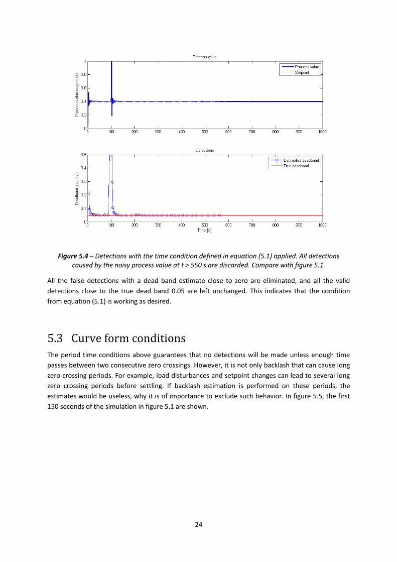
Figure 5.4 – Detections with the time condition defined in equation (5.1) applied. All detections caused by the noisy process value at t > 550 s are discarded. Compare with figure 5.1.
All the false detections with a dead band estimate close to zero are eliminated, and all the valid
detections close to the true dead band 0.05 are left unchanged. This indicates that the condition
from equation (5.1) is working as desired.
5.3 Curve form conditions
The period time conditions above guarantees that no detections will be made unless enough time
passes between two consecutive zero crossings. However, it is not only backlash that can cause long
zero crossing periods. For example, load disturbances and setpoint changes can lead to several long
zero crossing periods before settling. If backlash estimation is performed on these periods, the
estimates would be useless, why it is of importance to exclude such behavior. In figure 5.5, the first
150 seconds of the simulation in figure 5.1 are shown.

25
Figure 5.5 – Detections during a 150 second long simulation starting with a step at t=1 s and a load disturbance at t=100 s. The detections directly after these two disturbances are clearly too high, even
over 100% at t≈105 s.
In [4], Tore Hägglund proposes a condition in order to exclude these deviating detections. If εmax is
the largest error throughout the previous zero crossing period and Δy is the average error during the
same period, detections are accepted if and only if:
휀𝑚𝑎𝑥 < 2∆𝑦 (5.2)
Requiring that the maximum error must not exceed two times the average error puts a condition on
the shape of the error during the zero crossing period. For example, a perfect square wave has εmax =
Δy, while for a triangle, εmax = 2Δy. When backlash is present, the typical process output is similar to
a square wave, which without problem passes this condition. In reality, there is always an amount of
noise added to the signal, which directly affects εmax. The average amplitude Δy on the other hand, is
not affected by zero mean noise. This means that if the noise amplitude is very large, the condition
(5.2) will make sure that no detection is made. Fast setpoint changes can also be detected with (5.2),
as a change in ysp directly changes y. However, there are, or will be, other conditions for detecting
setpoint changes (see section 5.3).
The same simulation as in figure 5.5 but with condition (5.2) applied can be studied in figure 5.6:

26
Figure 5.6 – The condition εmax < 2Δy excludes the most deviating detection, but the reference step and the load disturbance are still affecting the dead band estimates.
Figure 5.6 shows that although the condition εmax < 2Δy excludes some detections, it does not
exclude enough. The remaining deviating detections can all be connected to decaying oscillations in
the process value. Figure 5.7 is a magnification of figure 5.6, which highlights the problem.

27
Figure 5.7 – Magnification of the decaying oscillation caused by the load disturbance at t=100 s. The
zero crossings are not a result of the backlash, and should therefore be neglected by the backlash dead band estimation algorithm.
Oscillation caused by backlash, see for example figure 5.3, is usually constant in amplitude. The
amplitude of a decaying oscillation is, as the name suggests, decaying. A simple way to detect this
unwanted behavior would be to compare the amplitude of the current zero crossing period with the
previous. If they are reasonably similar, it is likely caused by backlash. If the previous is larger than
the current with a given factor, the detection is neglected as a result of a decaying oscillation. For
example:
∆𝑦𝑝𝑟𝑒𝑣𝑖𝑜𝑢𝑠
∆𝑦 < 1.5, (5.3)
would only be true if the amplitude has decreased less than 50%. Applying this condition to the
simulation results in figure 5.8.
28
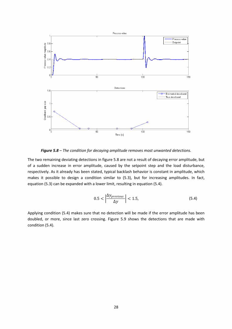
Figure 5.8 – The condition for decaying amplitude removes most unwanted detections.
The two remaining deviating detections in figure 5.8 are not a result of decaying error amplitude, but
of a sudden increase in error amplitude, caused by the setpoint step and the load disturbance,
respectively. As it already has been stated, typical backlash behavior is constant in amplitude, which
makes it possible to design a condition similar to (5.3), but for increasing amplitudes. In fact,
equation (5.3) can be expanded with a lower limit, resulting in equation (5.4).
0.5 <
∆𝑦𝑝𝑟𝑒𝑣𝑖𝑜𝑢𝑠∆𝑦
< 1.5, (5.4)
Applying condition (5.4) makes sure that no detection will be made if the error amplitude has been
doubled, or more, since last zero crossing. Figure 5.9 shows the detections that are made with
condition (5.4).

29
Figure 5.9 – Remaining detections after condition (5.4) is applied. Note the change of scale.
Testing shows that condition (5.4) works well for all processes in the test batch, meaning that it does
not affect correct detections significantly, yet it stops all erroneous detections caused by load
disturbances. It should be noted, however, that even when no load disturbance is acting on the
process, and no setpoint change is made, the error amplitude could indeed change more than what
condition (5.4) permits. This can lead to the loss of some proper detection, but this price is low and
must be paid.
It could be an advantage to let the operator set the lower and upper limits for condition (5.4), instead
of using the constant limits 0.5 and 1.5, respectively. This is not done in the final implementation of
this master thesis as it is reasoned that this would demand too much knowledge of the procedure
from the operator, without really contributing to the quality of the estimation. As the backlash
detection functionality is to be automatic, it must be kept as simple as possible.
5.4 Setpoint condition It is clear that the detections, both in manner of quality and quantity, depend a lot on the setpoint
value. It is of great importance to have insight in varieties caused by the setpoint, why simulations
with different setpoint forms have been done. A problem that can occur if the setpoint changes is
well illustrated in figure 5.10.

30
Figure 5.10 – Setpoint changes over time and give rise to faulty detections.
In the backlash estimation procedure, for calculating y, the control error is integrated between two
zero crossings. In this case the change of setpoint causes significantly higher detections compared to
the real dead band. A magnification of the zero crossing after 460 seconds is shown in figure 5.11,
which shows that it is directly related to the change of setpoint. Since the safety net of the
estimation procedure does not yet contain a condition for changes of the setpoint, the interval in the
figure gives rise to an incorrect detection, as the integrated error is much larger than it would be
without a change of setpoint.

31
Figure 5.11 – Zero crossings caused by a change of setpoint. The integrated error is the area bounded
by the set point and the process value.
In similar cases the detection will be eliminated by emax < 2y, but in this particular case the integral
error is large which leads to a backlash estimation of 13%, when the real value is 5%.
Similar problems can occur if a process is controlled with a slow and restrained controller.
Simulations with a noisy sine shaped setpoint were done, to replicate an external setpoint in an
industrial environment. The frequency of the setpoint signal is high and the controller parameters
restrained, which leads to a “chasing” process value, see figure 5.12.

32
Figure 5.12 – Process value and setpoint. The process value does not cross the setpoint until it changes direction.
Since the backlash estimation procedure integrates the error between the zero crossings, the
appearance in the figure is defined as backlash and provides poor estimations.
A solution to the problems, that also works on-line, is to compare the setpoint values between the
zero crossings. If the difference between the crossings is large relative to y, the detection is false
and should be eliminated. By eliminating detections the risk of estimating a false backlash is radically
reduced, but a longer time period is needed for an accurate result. The boundary
∆𝑦𝑠𝑝 < ∆𝑦 (5.5)
discovers large changes in setpoint and provides good results in both cases explained above. It is an
advantage that the boundary is simple and strict since the estimation procedure is to be automatic.

33
6. Implementation in ABB Control Builder
The backlash estimation procedure is implemented in ABB Control Builder as a control module in a
prototype library. Standard MatLab Simulink components, such as backlash and noise, are created for
simulations in Control Builder to work.
6.1 Control Builder The implementation part of the master thesis is made with ABB Control Builder Compact and will
result in a prototype library with the detection method as a control module. Control Builder is a
software used for PLC programming in an ABB 800xA environment. All the programming languages in
the international standard IEC 61131-3 can be used, such as Structured Text (ST), Ladder Diagram
(LD), Sequential Function Chart (SFC), Instruction List (IL) and Function Block Diagram (FBD) [6].
MatLab Simulink, used for simulations, and Control Builder are much alike, but there are some
central differences and several standard components missing in the latter. Therefore, for the model
to work, a couple of components had to be created, all programmed in structured text.
Control Builder uses blocks, so called control modules, for constructing simulation models. The
modules are connected to each other through nodes, also called Control Connections. The nodes can
send and receive information both forward and backward in the loop. The directional property of the
control connection is crucial in a real time environment, as it makes it possible to execute a control
loop in sequential order, each sample period. If every single component in the control loop would
calculate its output based on the input from last sample, the total time delay of the loop would be far
too long.
Not only the input and output to and from the control modules are shared over the control
connections. In addition, status signals are sent, indicating if some error has occurred in the loop.
This way, control modules can for example receive information about when a maximum or minimum
value has been reached.
For interacting with simulations in real time, every control module is connected to an interaction
window that allows the user to edit parameters, change modes, activate optional functionality etc.
6.2 NoiseCC For simulating noise in Control Builder a control module is created, called NoiseCC. A random
generator is used that provides a rectangular distributed range of random numbers between zero
and one. The implementation is done in structured text, see code block 6.1. The control module can
be connected anywhere in the control loop and requires only the amplitude of the noise.
NoiseCC – Control Module

34
Noise := (RandomRect(RandomGenerator) - 0.5) * 2;
Out.Forward.Value := In.Forward.Value + Power*Noise;
Code block 6.1 – Implementation of NoiseCC in Control Builder.
The variable Power is set by the user in the interaction window and corresponds to the size of the
noise amplitude. The control module, as it appears in Control Builder, can be seen in figure 6.1.
Figure 6.1 – Control module NoiseCC.
The noise is added to the input of the control module, and the sum is fed to the output.
6.3 BackLashCC The control module BackLashCC is created for representing a backlash in a Control Builder
environment. The module is easily implemented with an if-block programmed in structured text, see
code block 6.2. The variable deadband is given by the user in the interaction window and
corresponds to the size of the dead band.
BackLashCC – Control Module
if input > outputOld + deadband/2 then
output := input – deadband/2;
elsif input < outputOld – deadband/2 then
output := input + deadband/2;
else
output := outputOld;
end_if;
outputOld := output;
Code block 6.2 – Implementation of BackLashCC in Control Builder.
The module is implemented with the code above and is connected between the controller and the
process, with input u and output utrue.

35
Figure 6.2 – Control module BackLashCC.
Figure 6.2 shows the control module BackLashCC, as it appears in Control Builder.
6.4 BackLashDetectionCC BackLashDetectionCC is the main result of the master thesis and contains backlash detection,
estimation and compensation functions. With the reference signal and the process value as inputs
and the controller parameters known, a backlash can be detected and estimated as in equation (2.4).
As discussed in section 2.2, a compensation output signal is also created and may be connected to
the feed forward input on the controller. The stand-alone control module BackLashDetectionCC can
be seen in figure 6.3.
Figure 6.3 –Stand-alone control module BackLashDetectionCC.
The interaction window for the control module allows the user to control the backlash detection
procedure. The current dead band estimate is seen in the main interaction window together with
several operation buttons, see figure 6.4. The user can choose to view a graph with detections made
in time from the graph button and the input parameters to the control module can be changed in the
parameter interaction window. Finally the user has the possibility to compensate for the backlash by
pressing the compensate button, were the detections made after compensation are also viewed.

36
Figure 6.4 – Interaction window for BackLashDetectionCC with the current dead band estimate shown.
BackLashDetectionCC is currently implemented as a stand-alone control module with the controller
parameters received from the parameter interaction window. The control module could, in the
future, be implemented as a part of the standard Control Builder component PidAdvancedCC. The
module PidAdvancedCC is a controller used when more advanced functions than the ones
represented in PidCC are required.
6.5 Control Builder system A complete system is implemented, for simulations in Control Builder to work, and includes the same
complexity and functionality as in MatLab Simulink. The control modules are connected as in figure
6.5. Except for the control modules NoiseCC, BackLashCC and BackLashDetectionCC above, a couple
of standard components are being used. PidCC is a standard controller in Control Builder and
includes the controller parameters and basic control functions, such as the AutoTuner. ProcessSimCC
is a prototype module in the software and consists of two sections of low-pass filters with time delay.
The control module is used for simulating different types of processes in the test batch. The last
module Filter2PCC is another standard component in Control Builder and is, as the name indicates,
filtering the signal.
Figure 6.5 – Model constructed with Control Builder for simulating backlash in a control loop.

37
The figure shows how the process value changes over time, in the interaction window called InfoPar,
with backlash in the control loop. The dead band is set to 2.0% and the filtered detections when
compensation is inactive are 1.8%, which is considered to be a good result.
6.6 Final implementation As mentioned above, the functions in ABB Control Builder are implemented as separate modules that
can be connected using Control Connections. When new functionality is to be added, it must be
decided whether to add an additional module or expand an existing one. Some functions are
obvious; the BackLashCC module defined in section 6.3 should without doubt be implemented as a
new control module, while the AutoTuner-functionality was rightfully added to the PidCC module
instead of being implemented as a stand-alone module. Other functionality implementations are less
obvious.
The BackLashDetectionCC module has this far been referenced to as a stand-alone component. The
upside of this is that backlash detection is only added to a system when necessary. It also helps to
keep different functions clearly separated and therefore as simple as possible. The downside of a
detached implementation is that less information is available. If BackLashDetectionCC is
implemented as in figure 6.5, the controller parameters must be set manually. If the controller
parameters would change, for example after an AutoTuning has been preformed, they have to be
manually changed in BackLashDetectionCC. It can also be seen in figure 6.5 that two branches and
three Control Connections must be added to connect the BackLashDetectionCC. The input
connections are identical with those entering PidCC, hence the branches. It is clear that
BackLashDetectionCC could very well be implemented inside a PID-controller.
As it could not be decided within the time frame of this project how the final implementation should
be done, both possible alternatives are considered throughout the rest of this master thesis. It
should be mentioned that the BackLashDetectionCC as it is described here could easily be connected
inside a PID-control module such as PidCC, or more likely PidAdvancedCC.

38
7. Investigation and analysis
During the completion of this master thesis, several unanswered questions appeared. Many of these
questions had an intuitive answer, but had not been proved. Such proofs and verifications are
collected in this chapter, together with some functionality that was added to the detection procedure
during the final stages of the project.
7.1 Saturation of control signal When controlling a process with a PI-/PID-controller, the control signal is calculated as:
𝑢 = 𝐾 −𝑦𝑠𝑝 +1
𝑇𝑖 𝑦𝑠𝑝 − 𝑦𝑓 𝑑𝑡 − 𝑇𝑑𝑦 𝑓 𝑡 𝑡
0
.
Even if the setpoint and process value are limited within a certain interval, which usually is the case,
the control signal can be unlimited, due to the integral action. Even though the control signal in
theory might be infinitely large, there are physical limits on the actuators and control hardware. In
this case the ABB 800xA system works with signals in the range 4 to 20 mA. This means that in reality,
the control signal is indeed limited, i.e. it may become saturated.
The backlash dead band estimation algorithm that is the topic of this paper is sensitive to saturation.
As explained in section 2.1, the dead band is estimated based on how much control signal is needed
in order to drift through the dead band. The change of control signal between two zero crossings,
Δu, gives an approximate estimate of the dead band and can be written as:
∆𝑢 ≈
𝐾
𝑇𝑖∆𝑦∆𝑡. (7.1)
For this equation to hold, it is assumed that the control signal is not saturated. If saturation is present
and is affecting the control signal, erroneous detections will be produced. In figure 7.1, a simulation
with saturated control signal is shown.

39
Figure 7.1 – Erroneous detections caused by a strongly saturated control signal.
As it can be seen in figure 7.1, the dead band detections are more than ten times as large as the true
dead band (0.05 = 5 %). This is a direct effect of the saturation. Since the control signal is saturated, it
will take longer time to drift through the dead band than it would if the control signal was unlimited
in magnitude. The extra time it takes to cross the dead band directly effects the estimated dead
band, as the estimation is proportional to the time Δt.
When saturation is present, action needs to be taken. The first step is to identify that the control
signal has been limited by saturation to some extent during the last zero crossing interval. This can be
done in several ways, depending on how the estimation procedure is to be implemented.
The most problematic situation is if the backlash detection is implemented as a stand-alone control
module, with y and ysp as only inputs. If this is the case, the only knowledge of the control signal is
its relative change during the zero crossing period Δu, calculated according to equation (7.1). If this
change is larger than the control signal span, umax–umin, then obviously the control signal has been
more or less saturated. This requires information of the parameters umin and umax, but these are
usually 0 and 100, respectively. In figure 7.2, this condition is used to filter out detections.

40
Figure 7.2 – Detections with saturated control signal. Some detections are removed with the
condition Δu < umax – umin. Compare with figure 7.1.
As it can be seen in figure 7.2, this condition is insufficient. If backlash detection is to be
implemented as a feature of the PidAdvancedCC control module many doors open, as discussed in
section 6.6. This includes direct access to the control signal, the umin/umax-variables and the
saturation status of the controller. Thus, the question of whether or not the controller is saturated
can be answered in two ways. The straight forward approach, to check if the control signal u has
reached umax or umin during the zero crossing period, is perhaps the least advantageous. It would of
course be very useful, and eliminate all detections from figure 7.1, but only saturation of the
controller itself would be detected. It would not, for example, notice if a slave controller in a cascade
loop saturated or if an actuator has reached its end position.
The second approach is to monitor the saturation status of the controller. Recall section 6.1, where
the Control Connection tool in Control Builder is described. When some part of a control loop
reaches its minimum or maximum value, the flag MinReached or MaxReached is sent backwards
in the control loop. If a flag is received, or sent, by the controller, some saturation is present in the
control loop, and the safest action to take for the estimation procedure is to neglect the following
detection. By doing so it is made sure that no saturation of any part of the control loop affects the
estimated backlash gap. As every control module has a responsibility to pass on the saturation-flags,
it is sufficient to supervision the saturation status of the control connection connected to the feed
forward input of controller. By implementing this, all backlash estimations in figure 7.2 would be
eliminated.

41
7.2 The process parameter Kp
In a perfect plant, in a perfect world, every process model would be known by the operator. This is
unfortunately not the case. In the real world, rather few process parameters are available. On the
other hand, since most industrial processes are controlled with PI-/PID-controllers no exact process
model is needed to obtain satisfactory closed loop behavior [7]. If a procedure like the one described
in [4] is to be used, as little information about the process as possible should be required. In section
2.1 it is stated that the only information about the process that must be known is the static process
gain, Kp. Even this parameter could be unknown to the operator, why it is of interest to investigate
how much the algorithm is influenced by errors in the Kp-parameter.
7.2.1 The influence of Kp
The estimated dead band was derived in 2.4 as
𝑑 =
𝐾∆𝑦∆𝑡
𝑇𝑖−∆𝑦
𝐾𝑝= 𝐾∆𝑦
∆𝑡
𝑇𝑖−
1
𝐾𝐾𝑝 . (7.2)
This equation is clearly separated in two parts, one independent of Kp and one dependent of Kp. The
safety net condition for zero-crossing period time guarantees that:
∆𝑡 > 5𝑇𝑖, (7.3)
and thus the Kp -independent part of the backlash estimate:
∆𝑡
𝑇𝑖> 5
If the controller is well tuned the product KpK is limited [3]:
0.5 < 𝐾𝐾𝑝 < 1,
1 <1
𝐾𝐾𝑝< 2.
(7.4)
Still, the contribution from the Kp-part can in the worst case be as large as 40% of the detection
value. This shows that Kp is an important parameter that can cause large errors in detections if not
correctly set.
In practice, the zero-crossing time period is in most cases much longer than 5Ti. This suggests that
the contribution from Kp is actually seldom as large as 40% of the detection value. Figure 7.3 and 7.4
indicates a typical influence of Kp during simulation, where Kp equals 1 and the controller gain is 1.2.

42
Figure 7.3 – The Kp-independent part (red) of the backlash estimate is considerably larger than the Kp-dependent part (green). This suggests that the method is more insensitive to deviations in Kp than
equations (7.2) – (7.4) implies.
Figure 7.4 – The quotient between the Kp-dependent and Kp-independent part of the backlash estimate never exceeds 10% in this simulation, as opposed to the worst case 40% from theory.
43
7.2.2 A default value of Kp
If the static gain is unknown a default value is needed in order for the algorithm to run. In [4], it is
suggested to use a default value of 1.5, as most industrial processes use normalized signals with Kp ≈
1. This default value, it is stated, results in a detection error of less than 20%, under the assumption
that the true process gain is between 1 and 3.4 [4].
As discussed in 6.6, the backlash detection algorithm might very well be implemented in the
PidAdvancedCC control module. PidAdvancedCC is a PID-controller with added functionality such as
gain scheduling, setpoint ramping and AutoTuner. The AutoTuner is a function for automatic
estimation of suitable PID-parameters [8]. The Autotuner algorithm calculates the static process gain,
which it then uses to calculate suitable controller parameters. This value of Kp can be used in the
backlash detection algorithm if autotuning has been performed.
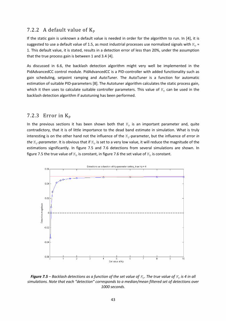
7.2.3 Error in Kp
In the previous sections it has been shown both that Kp is an important parameter and, quite
contradictory, that it is of little importance to the dead band estimate in simulation. What is truly
interesting is on the other hand not the influence of the Kp-parameter, but the influence of error in
the Kp-parameter. It is obvious that if Kp is set to a very low value, it will reduce the magnitude of the
estimations significantly. In figure 7.5 and 7.6 detections from several simulations are shown. In
figure 7.5 the true value of Kp is constant, in figure 7.6 the set value of Kp is constant.
Figure 7.5 – Backlash detections as a function of the set value of Kp. The true value of Kp is 4 in all
simulations. Note that each “detection” corresponds to a median/mean filtered set of detections over 1000 seconds.

44
Figure 7.6 – Backlash detections as a function of the true value of Kp. The set value of Kp is 4 in all
simulations.
From figure 7.5 it can be concluded that setting the Kp parameter very low can lead to very small
detections, even less than zero in the extreme case. In this set of simulations, a too high value of Kp
leads to even better detections than the correct value. Figure 7.6 indicates that if the set value of Kp
is large enough, a change of the true Kp-value must be very large before affecting the estimations. It
should be noted that no value of Kp leads to too large backlash estimates in these simulations.
Therefore, the value of Kp can never lead to an over compensated system, which is an important
conclusion for the methods robustness.
7.3 Filtering of detections The procedure described in [4] calculates a backlash estimate every time a zero-crossing occurs if the
safety net conditions from chapter 5 are fulfilled. These estimates will hopefully be reasonably
similar, indicating that the estimates are of good quality. Regardless of how similar the estimates are,
only one value should be displayed to the operator for the method to be functional and simple
enough to be used. To simply display the mean value of all previous detections is a possibility, but
one with several flaws.
Chapter 5 defines a set of conditions designed to assure that detections are only calculated when
there is a backlash behavior in the control loop. These conditions have been proved efficient in
simulation, but when running the method online anything can happen. When something indeed does
happen, meaning that a detection is calculated under non-typical circumstances, the calculated

45
backlash estimate will mostly often be far from the estimates calculated under normal conditions.
Figure 7.7 shows a set of detections from a simulation where some detections are clearly erroneous.
Figure 7.7 – Backlash estimates over time.
The deviating detections in figure 7.7 will affect the mean value. Preferably, deviating detections
should not in any way be allowed to influence the mean value. This can be achieved using a median
filter approach [9]. A median filter is a non-linear digital filter with good noise suppression
properties. The median filter value can be generally defined as:
𝑦 𝑘,𝑁 = 𝑚𝑒𝑑𝑖𝑎𝑛 𝑥 𝑘 +𝑁
2 , 𝑥 𝑘 +
𝑁
2− 1 ,… , 𝑥 𝑘 ,… , 𝑥 𝑘 −
𝑁
2+ 1 , 𝑥 𝑘 −
𝑁
2 ,
where N is the size of the filter window. This implementation is not optimal for the backlash
estimates since no detected value is probable to be exact. However, the median filter idea can be
used to eliminate deviating detections like the ones in figure 7.7. The filter used in the remainder of
this master thesis has the following properties:
1. The median of the N last detections is calculated
2. All detections larger than 120% or smaller than 80% of the median are discarded
3. The mean value of the remaining detections is calculated and displayed
This filter provides a robust dead band estimate, uninfluenced by deviating detections. The filter size,
N, could be set by the operator during operation or static. As N detections need to be made for a
value to be displayed, a large value of N results in a delay. On the other hand, a small filter size can
lead to unsmooth filter output as the median is calculated from fewer estimates. Figure 7.8 indicates

46
the drawback of pure mean filtering, while figures 7.9 and 7.10 highlight the influence of the filter
window size N.
Figure 7.8 – Mean value of detections. The sudden change of estimate magnitude affects the mean
value slowly.

47
Figure 7.9 – Median/mean filtering with filter window size N=5. The delay is short, but the filter output could be smoother.
Figure 7.10 – Median/mean filtering with filter window size N=15. Longer delay than with N=5, but
smoother filter output.
From figure 7.10 it is clear that a large value of N, in this case N=15, leads to a delay. It is on the other
hand not very likely that the backlash estimates would change in such a sudden way as in these
figures. In the implemented version of the filter, a filter width of N=9 is used. N should always be an
odd number, otherwise the median value is calculated as a mean value of the two most centered
estimates, which can lead to that no estimate is within 80% and 120% of the median.
7.4 Over compensation detection By compensating for a backlash the mechanical parts in the process can be used for a longer time
before they have to be replaced or repaired, which is important for economical reasons. As discussed
in 2.2, the compensation procedure is implemented by jumping trough the dead band every time the
control signal is reversed. The feed forward signal,
𝑢𝐹𝐹 =𝛿
2𝑠𝑖𝑔𝑛 𝑒 ,
to the controller is implemented as an additional function to the estimation procedure. The user can
choose to compensate for the entire amount of the estimated dead band or only parts of it.
Compensating for less than the real dead band results in an under compensation and does not
eliminate the typical backlash behavior in the control loop. The amount of backlash is reduced, but

48
not eliminated when under compensated. When over compensated, the controller can be modelled
as a linear PID-controller and a nonlinear part caused by the compensation from the feed forward
input, see figure 7.11. The nonlinear part can be described as a relay, with amplitude depending on
the size of the over compensation. If the over compensation is large the relay is dominating the
system, which can cause a limit cycle to arise.
Figure 7.11 – A controller modelled as a linear PID-controller and a nonlinear part described as a relay when over compensated.
Since the dominating reason for the limit cycle is the relay part, the controller is removed as in figure
7.12 for an analysis of the system.
Figure 7.12 – The controller is removed for an analysis of the system.
A relay followed by a backlash equals a relay with lower amplitude since the control signal from the
relay has to drift through the dead band when reversed, that is
𝐴𝑟𝑒𝑙𝑎𝑦 =𝑐𝑜𝑚𝑝𝑒𝑛𝑠𝑎𝑡𝑖𝑜𝑛 − 𝑑𝑒𝑎𝑑𝑏𝑎𝑛𝑑
2.
A possible limit cycle will arise if the negative inverse of the describing function of a relay and the
Nyquist diagram of the process intersect. The describing function of a relay is rather simple, and real
𝑁 𝐴 =4𝐴𝑟𝑒𝑙𝑎𝑦
𝜋𝐴.
For a complete analysis the process must be known, however, this is not the case in the backlash
estimation procedure. The negative inverse of the describing function of a relay can be seen in a
Nyquist diagram as a line from zero to minus infinity. All processes with a Nyquist curve crossing the
negative real axis will therefore cause a possible limit cycle, with unknown amplitude and frequency,
when over compensated. All stable systems with pole excess larger than two (number of poles –
number of zeros) or with time delay will have such a Nyquist curve. When compensation is active,
limit cycles can be detected and warned for in a rather simple way. By comparing the time period for

49
zero crossings, oscillations with a constant frequency can be detected. The system oscillates if the
time periods between the zero crossings are constant, that is t=t1=t2=…=tn. If the maximum
difference between the four last t is less than two times the sample rate when compensation is
active, an indicator is shown in the interaction window. The over compensation method is
implemented as
if max(ti+3, ti+2, ti+1, ti)–min(ti+3, ti+2, ti+1, ti) < 2h then
OverCompensationWarning := true;
end_if;
Code block 7.1 – Implementation of over compensation warning.
This is an effective method that also works on-line if the last four t are being saved.
7.5 Derivative action In process industry, as much as 97% of the control loops use PI-control [7]. Of the remaining three
percent, some are controlled with state feedback controllers, some with adaptive controllers, some
with PID-controllers and so on. The procedure analyzed in this master thesis is implemented for use
with a PI-/PID-controller, as this is clearly the most common case. To prove that the algorithm is
applicable for PID-controllers, some questions must be answered.
The backlash detection algorithm estimates the dead band based on how much the control signal has
changed between two zero crossings. This change, Δu, can be written as:
∆𝑢 = 𝑢𝑖+1 − 𝑢𝑖 =
= 𝐾 −𝑦𝑠𝑝 +1
𝑇𝑖 𝑦𝑠𝑝 − 𝑦𝑓 𝑑𝑡 − 𝑇𝑑𝑦 𝑓 𝑖 + 1 𝑖+1
0
− 𝐾 −𝑦𝑠𝑝 +1
𝑇𝑖 𝑦𝑠𝑝 − 𝑦𝑓 𝑑𝑡 − 𝑇𝑑𝑦 𝑓 𝑖 𝑖
0
=
=𝐾
𝑇𝑖 𝑦𝑠𝑝 − 𝑦𝑓 𝑑𝑡
𝑖+1
𝑖
− 𝐾𝑇𝑑 𝑦 𝑓 𝑖 + 1 − 𝑦 𝑓 𝑖 ,
if a PID-controller on the form (4.1) is used. The integral part can then be rewritten, using the
average error instead of the integral:
𝛥𝑦𝛥𝑡 = 𝑦𝑠𝑝 − 𝑦𝑓 𝑑𝑡𝑖+1
𝑖
.
If the controller is a pure PI-controller, we get the expression:
∆𝑢 =𝐾
𝑇𝑖∆𝑦∆𝑡. (7.5)
If there is derivative action in the controller however, this expression is not true. In the original paper
by Tore Hägglund the contribution from the derivative part of the controller is neglected, and Δu is

50
approximated as expression (7.5) regardless of if there is derivate action present. With derivative
action, Δu is given by equation (7.6):
∆𝑢 =𝐾
𝑇𝑖∆𝑦∆𝑡 − 𝐾𝑇𝑑 𝑦 𝑓 𝑖 + 1 − 𝑦 𝑓 𝑖 . (7.6)
It must be shown that expression (7.6) is almost the same as expression (7.5). To start with, the
derivatives are approximated as of equal magnitude but alternating signs:
𝑦 𝑓 𝑖 + 1 = 𝑦 𝑓 𝑖 → 𝑦 𝑓 𝑖 + 1 − 𝑦 𝑓 𝑖 = ±2 𝑦 𝑓 𝑖 →
∆𝑢 = 𝐾 ∆𝑦∆𝑡
𝑇𝑖± 2𝑇𝑑 𝑦 𝑓 𝑖 .
|𝑦 𝑓 𝑖 | = |Δ𝑦𝑓
Δ𝑡| =
Δ𝑦𝑓
Δ𝑢∙Δ𝑢
Δ𝑡 ,
but by assuming that the signals are changing slowly the process dynamics can be neglected, and
Δyf=KpΔu:
𝑦 𝑓 𝑖 = 𝐾𝑝 ∙Δ𝑢
Δ𝑡 ,
and thus:
∆𝑢 = 𝐾 ∆𝑦∆𝑡
𝑇𝑖± 2 ∙ 𝑇𝑑 ∙ 𝐾𝑝 ∙
Δ𝑢
Δ𝑡 →
∆𝑢 1 ±2 ∙ 𝐾 ∙ 𝑇𝑑 ∙ 𝐾𝑝
Δ𝑡 =
𝐾
𝑇𝑖∆𝑦∆𝑡.
It must now be shown that:
2 ∙ 𝐾 ∙ 𝑇𝑑 ∙ 𝐾𝑝
Δ𝑡≪ 1.
The derivative gain Td is never larger than Ti/4, if the controller is properly tuned. For example, the
Autotuner always sets Ti=6.25Td [10], and the Ziegler-Nichols methods sets Ti=4Td [5]. It is also
known that the zero crossing period Δt > 5Ti. Inserting this gives:
2 ∙ 𝐾 ∙ 𝑇𝑑 ∙ 𝐾𝑝
Δ𝑡<
2 ∙ 𝐾 ∙ 𝑇𝑑 ∙ 𝐾𝑝
5 ∙ 4 ∙ 𝑇𝑑=
2 ∙ 𝐾 ∙ 𝐾𝑝
20.
As stated in equation (7.4), the product KpK is limited between 0.5 and 1. This proves that in the
worst case,
2 ∙ 𝐾 ∙ 𝑇𝑑 ∙ 𝐾𝑝
Δ𝑡<
2
20= 10%,
which means that the error caused by the approximation:
∆𝑢 ≈𝐾
𝑇𝑖∆𝑦∆𝑡

51
is less than 10%. With this being proved, it is safe to use the approximation in the backlash
estimation algorithm.
It should also be mentioned that the error caused by the approximation is alternating between
positive and negative, with similar magnitude. The filter defined in section 7.3 will therefore
smoothen the error out.

52
8. Testing
The only way to guarantee the robustness of the backlash estimation procedure and find out if the
safety net is sufficient is by performing tests and simulations. In this chapter different tuning
methods, cascaded control and systems with dead time are tested. Simulations on all processes in the
test batch are performed and finally real industrial tests are made.
8.1 Test of test batch The test batch contains eight different processes, all suitable for PID-controllers. Lag dominated,
delay dominated, balanced and integrating processes have all been tested with the backlash
estimation procedure with satisfying results. All processes are controlled with PI-/PID-controllers
with controller parameters obtained from the MIGO tuning rules. Simulations with various dead
bands are made on the processes and presented in figure 8.1.

53
Figure 8.1 – Simulations of all processes in the test batch with various dead bands. The dashed line (red) corresponds to a correct dead band estimation and the solid line (blue) the median filtered dead
band estimate.
The figures above correspond to the eight processes in the test batch simulated with various dead
bands. The red dashed line in the figures represents a perfect estimation, in other words when the
estimated dead band equals the true dead band. The solid blue line corresponds to the actual
estimations obtained with the backlash estimation procedure. The simulations show that the
estimations are slightly lower than the true dead band or equal to zero for all processes in the test
batch. This is a good property, since it is important that the backlash compensator does not use an
estimate that is too high.
The fact that no detections are made for several processes is caused by the lack of backlash behavior
in the process value. The first process P1 is an integrating process that causes a limit cycle to arise if
backlash is present in the control loop. P4 is a system with significant time delay and P8 a delay-
dominated process, both hard to control. This results in restrained controller parameters with less
impact on backlash and as a result less detections. The backlash estimation procedure provides in
general satisfying results and works on-line for all processes in the test batch.

54
8.2 Tuning Methods
Different types of tuning methods and controllers provide dead band estimates with various
accuracy. By choosing an advanced tuning method, the detections obtained from the estimation
procedure can be drastically improved. A number of simulations, with various controllers and tuning
methods, are presented in table 8.1. The simulations are made on process P2 from the test batch
with a dead band of 5% during 5000 seconds.
𝑷(𝒔) =𝟏
𝟏 + 𝒔 𝟒
d = 5%
Estimated d (%) /
Number of detections
Estimated d (%) /
Number of detections
PI PID
Ziegler-Nichols frequency
4,22 % / 8 2,79 % / 55
Lambda --- 4,49 % / 3
MIGO, M=1.4 --- 4,39 % / 77
AMIGO step. --- 3,90 % / 39
AMIGO frequency --- 4,10 % / 77
Table 8.1 – Simulations during 5000 seconds with various controllers and tuning methods.
The table shows that the backlash estimation procedure works with all tuning methods. Ziegler-
Nichols is a rather aggressive procedure and provides the least accurate results, but is still precise for
its simplicity.
The low number of detections when using Lambda tuning is not a coincidence. The slow, or sluggish,
control obtained from the Lambda tuning results in long zero crossing intervals when there is
backlash present in the loop. This is a direct effect of the controller tuning, as the time it takes to
drift through the dead band is proportional to the quotient Ti/K. As table 8.1 shows, the detections
made with a Lambda tuned controller are the most precise. As the zero crossing periods are long, the
effects of round off and noise are minimized. These characteristics – few but accurate detections –
are typical for slow controllers. However, if the controller is too slow, the amount of detections can
be reduced to zero. Figure 8.2 shows the result from a simulation with a very sluggish controller.

55
Figure 8.2 – Simulation with very sluggish controller during 10 000 s. The process value is always close enough to the setpoint for the noise to cause zero crossings.
As figure 8.2 clearly shows, the average control error is smaller in magnitude than the noise. The
average control error, denoted Δy throughout this thesis (see figure 2.1), can be seen as an
overshoot that occurs when the backlash gap is crossed. If the controller is slow, the process value
only changes a little before the control action is reversed. No detections are made during the
simulation in figure 8.2, as the noise causes zero crossings that does not fulfill the zero crossing time
interval condition defined in section 6.2. A possible solution to this problem would be to increase the
feedback filter time, Tf, which by default is set as Tf = Ti/2.
The lack of detections when PI-control is used is caused by the lack of backlash behavior in the
process value. This is directly related to the process and should not be seen as an overall conclusion.
Figure 8.3 shows process P2 being controlled with various tuning methods and with backlash in the
control loop.

56
Figure 8.3 – Step responses for process P2 obtained from various tuning methods with backlash in the control loop.
The simulation with the controller parameters obtained from the Ziegler-Nichols method, provided a
large number of detections, but not very accurate ones. The tuning is, as figure 8.3 suggests, too poor
to achieve desired closed loop behavior. It takes a very long period of static setpoint for the process
value to stop oscillating. These oscillations affect the backlash estimation.
MIGO and approximate MIGO are both relatively advanced tuning methods that provide very good
controllers which leads to accurate estimations. The methods result in many detections, where the
estimation obtained from the approximate MIGO is slightly lower than for the original method.
8.3 Cascade control
Some processes are difficult or impossible to control with a simple PI-/PID-controller [3]. In those
cases, a more sophisticated control strategy is needed. If the process model is known, state feedback
can be used to efficiently place the closed loop poles in their desired positions. Other strategies
include model predictive control and internal model control. In process industry, it is a rarely seen
luxury to be in possession of an exact model of the process to be controlled, why it is impossible to
use these model based control strategies. Even so, the concept of state feedback can be used with
well tuned PI-/PID-controllers to obtain a stable system. This results in a cascade control system,
where one controller provides a setpoint for the next one. In order to use cascade control, the
process must be dividable into two or more parts, and the process value must be measurable in each
junction. If the measurable signals corresponds to the state variables, cascade control is in fact
equivalent to state feedback [3], and as such, the closed loop system poles can be placed arbitrarily
under the assumption that the process is controllable [5].

57
8.3.1 Backlash on the input of the inner process
If cascaded control is used, the reference to the “process input” becomes ambiguous. As the process
model is split into two or more parts, each with both an input and an output. The parts can be
separated into being either an inner or an outer process. The fundamental difference lies in the fact
that inputs of inner processes are directly connected to a controller, while as outer processes receive
their input signals from the output of another process. There can only be one inner process in a
cascade control system, but the number of outer processes are unlimited.
Figure 8.4 shows a Simulink model of a two-stage cascade control system with backlash on the inner
process input.
Figure 8.4 – Two stage cascade control loop in Simulink. The inner process is subject to backlash on
the input.
It is of interest to find out how the detection algorithm handles backlash in a cascaded control loop.
To test this, process P2 from the test batch,
𝑃2 =1
𝑠 + 1 4 ,
is rewritten as two processes,
𝐺𝑝1 =1
𝑠 + 1 2 ,
𝐺𝑝2 =1
𝑠 + 1 2 ,
such that
𝑃2 = 𝐺𝑝1 ∙ 𝐺𝑝2 .
Now, process P2 can be controlled using cascaded control. Note that the controller parameters have
to be recalculated to provide satisfactory closed loop behavior. Simulation of the cascaded system
with a step reference and load disturbance at t=100 s is given in figure 8.5.
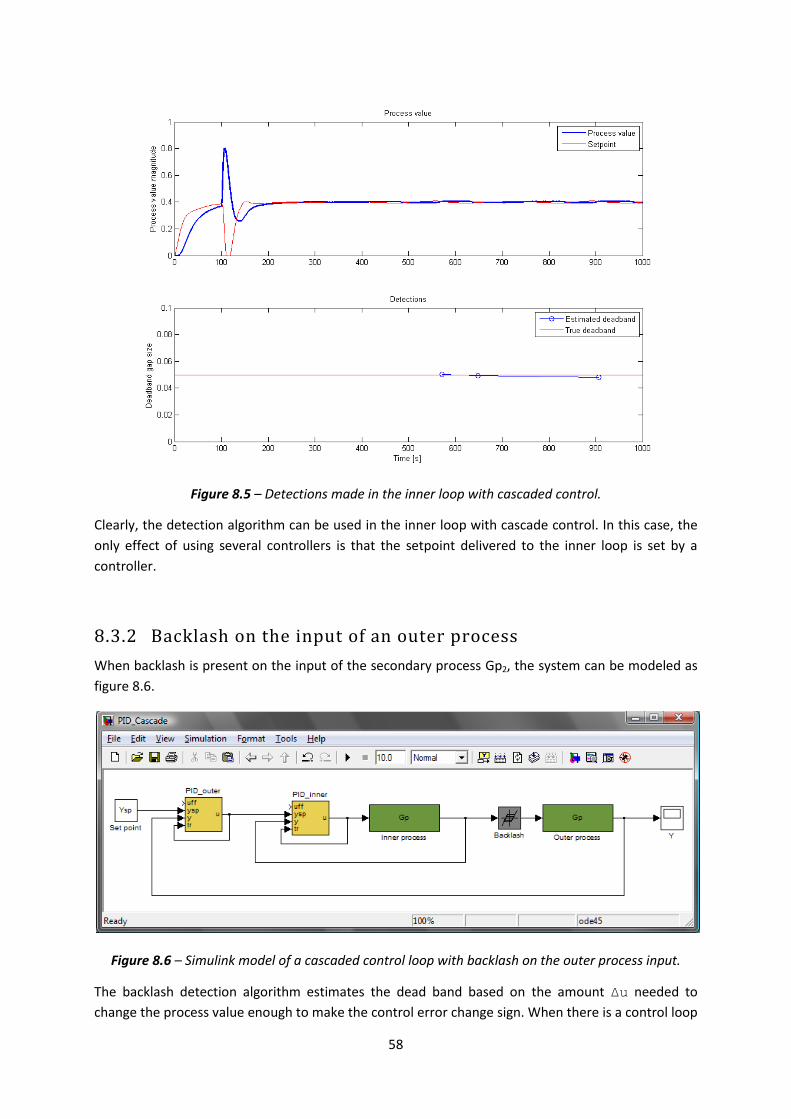
58
Figure 8.5 – Detections made in the inner loop with cascaded control.
Clearly, the detection algorithm can be used in the inner loop with cascade control. In this case, the
only effect of using several controllers is that the setpoint delivered to the inner loop is set by a
controller.
8.3.2 Backlash on the input of an outer process
When backlash is present on the input of the secondary process Gp2, the system can be modeled as
figure 8.6.
Figure 8.6 – Simulink model of a cascaded control loop with backlash on the outer process input.
The backlash detection algorithm estimates the dead band based on the amount Δu needed to
change the process value enough to make the control error change sign. When there is a control loop

59
between the outer controller and the backlash, the control signal is distorted before it reaches the
backlash. Because of this, it is impossible to make an accurate estimation of the backlash, as the
input to the backlash cannot be predicted. This insight states a fundamental limitation of the
detection procedure; detections can only be made in the inner loop of a cascade control system.
Fortunately, it is not very likely that backlash is present on the input of the outer process. Typically, in
process industry, the inner process is a valve while the outer is a tank, and it is the valve that is
affected with backlash.
8.4 Dead time In industrial control systems, time delays are always a problem. Time delay, or dead time, can be
caused by long signal paths, feedback loops, computation time etc. These signal related dead times
are however very short compared to physical ones, such as the time it takes for a flow of paper mass
to reach from a newly opened valve to the tank level. In the worst case, these dead times can be as
long as minutes or hours.
8.4.1 Dead time and backlash
In a sense, backlash can be seen as a special type of time delay. The delay is not constant, and only
shows when the control signal changes direction, e.g. from increasing to decreasing. As a large
backlash leads to longer delay times, it is not unreasonable to suspect that internal process dead
times can affect the estimated backlash.
Figure 8.7 shows how backlash estimates relate to the process dead time. In the simulations, process
P2 and P3 from the test batch is used, with added time delay, that is:
𝑃2+𝑑𝑒𝑙𝑎𝑦 𝑠, 𝐿 =1
𝑠 + 1 4𝑒−𝑠𝐿 ,
𝑃3+𝑑𝑒𝑙𝑎𝑦 𝑠, 𝐿 =9
𝑠 + 1 (𝑠2 + 2𝑠 + 9)𝑒−𝑠𝐿 ,
where L is the time delay in seconds. The controller parameters have been recalculated for every
value of L, using the software designPID [8], to eliminate the effects of improper tuning.

60
Figure 8.7 – Average backlash estimates as a function of process time delay L.
From figure 8.7 it can be concluded that dead time affects the estimation procedure considerably.
For long time delays, no detections are made at all. This is a fact since the controller is tuned to be
very moderate not to risk the closed loop stability when there is a long time delay within the process.
In section 8.2 it was shown that too sluggish control leads to a loss detections. This is why no
detections are made when there is a long time delay in the system. Figure 8.8 shows how the process
value behaves in a 20 000 seconds long simulation with 15 seconds delay on the process input.

61
Figure 8.8 – Process value with long dead time
As discussed in section 8.2, a change of filter time constant Tf could solve this problem. Figure 8.9
shows how an increase of filter time constant with a factor 4 affects the process value.
Figure 8.9 – Process value with increased filter time constant, compare with figure 8.8.
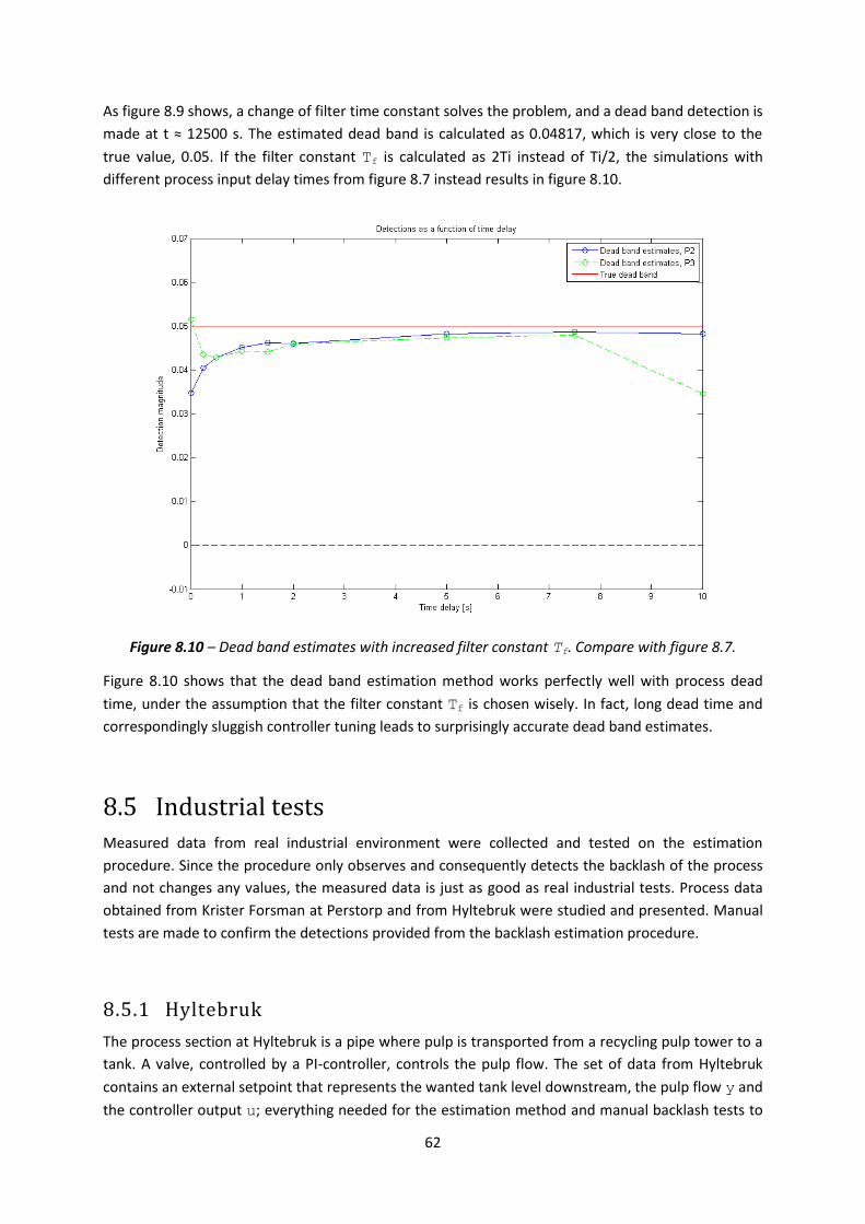
62
As figure 8.9 shows, a change of filter time constant solves the problem, and a dead band detection is
made at t ≈ 12500 s. The estimated dead band is calculated as 0.04817, which is very close to the
true value, 0.05. If the filter constant Tf is calculated as 2Ti instead of Ti/2, the simulations with
different process input delay times from figure 8.7 instead results in figure 8.10.
Figure 8.10 – Dead band estimates with increased filter constant Tf. Compare with figure 8.7.
Figure 8.10 shows that the dead band estimation method works perfectly well with process dead
time, under the assumption that the filter constant Tf is chosen wisely. In fact, long dead time and
correspondingly sluggish controller tuning leads to surprisingly accurate dead band estimates.
8.5 Industrial tests Measured data from real industrial environment were collected and tested on the estimation
procedure. Since the procedure only observes and consequently detects the backlash of the process
and not changes any values, the measured data is just as good as real industrial tests. Process data
obtained from Krister Forsman at Perstorp and from Hyltebruk were studied and presented. Manual
tests are made to confirm the detections provided from the backlash estimation procedure.
8.5.1 Hyltebruk
The process section at Hyltebruk is a pipe where pulp is transported from a recycling pulp tower to a
tank. A valve, controlled by a PI-controller, controls the pulp flow. The set of data from Hyltebruk
contains an external setpoint that represents the wanted tank level downstream, the pulp flow y and
the controller output u; everything needed for the estimation method and manual backlash tests to
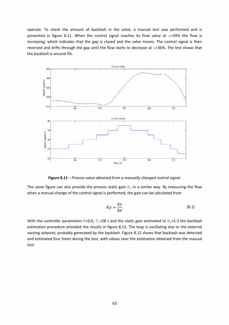
63
operate. To check the amount of backlash in the valve, a manual test was performed and is
presented in figure 8.11. When the control signal reaches its final value at u≈39% the flow is
increasing, which indicates that the gap is closed and the valve moves. The control signal is then
reversed and drifts through the gap until the flow starts to decrease at u≈36%. The test shows that
the backlash is around 3%.
Figure 8.11 – Process value obtained from a manually changed control signal.
The same figure can also provide the process static gain Kp in a similar way. By measuring the flow
when a manual change of the control signal is performed, the gain can be calculated from
𝐾𝑝 =
∆𝑦
∆𝑢.
(8.1)
With the controller parameters K=0.6, Ti=28 s and the static gain estimated to Kp=1.3 the backlash
estimation procedure provided the results in figure 8.12. The loop is oscillating due to the external
varying setpoint, probably generated by the backlash. Figure 8.12 shows that backlash was detected
and estimated four times during the test, with values near the estimation obtained from the manual
test.

64
Figure 8.12 – Process value and estimated detections obtained with an external setpoint from
Hyltebruk.
Experiments with an internal setpoint were also performed, to avoid setpoint variations that may
disturb the backlash estimation. Figure 8.13 shows the results obtained with the internal setpoint,
where the oscillations caused by the setpoint variations have disappeared. The three backlash
detections made during the test are slightly lower than in the previous example. This can be
expected since setpoint variations amplify the effect of the backlash.

65
Figure 8.13 – Process value and estimated detections obtained with an internal setpoint from Hyltebruk.
8.5.2 “Perstorp”
The process data obtained from Krister Forsman at Perstorp contains the setpoint value, the process
value and the control signal, but the controller parameters and the static process gain Kp are not
known. By using a MatLab script, designed by Krister Forsman, the controller parameters can be
obtained from the process data only. The script provided a PI-controller with parameters K=8.5 and
Ti=10.3 s. The estimation procedure requires the static gain of the process as well; this can be
obtained from the process data, see figure 8.14.

66
Figure 8.14 – The process value obtained from a manually changed control signal.
Figure 8.14 shows a manually changed control signal. After t=2500 s the control signal is reversed and
drifts through the gap. Kp is then given by the step at t=3097 s, see equation (8.2).
𝐾𝑝 =
∆𝑦
∆𝑢=
0.92
2= 0.46
(8.2)
The backlash can be manually estimated in the same figure by observing the change in the process
value over time. When the control signal is reversed at t=2500 s, it takes another 300 s for the
process value to change. The control signal drifts from 20 to 45 during the same time period, this
indicates that the gap is around 25. The backlash estimation procedure, with the controller
parameters K=8.5, Ti=10.3 s and the static gain Kp=0.46, provides the results in figure 8.15. Several
detections are made and estimated around 22; the manually changed signal confirms the result.

67
Figure 8.15 – Process value and estimated detections.
The results from the industrial tests confirm that the backlash estimation procedure works
automatically in an industrial environment. By detecting and estimating the backlash on-line during a
longer time period, a more accurate estimation can be obtained. The estimations provided by the
manual tests are not as precise as the real detections, but still confirm the amount of backlash in the
control loop.
68
9. Conclusions and future work This chapter covers the main conclusions made during this project, which give answers to the initial
objectives described in section 3.1. Future work that could improve the backlash estimation procedure
is also studied.
The initial objectives, described in chapter 3, of the project have been answered and expanded in this
thesis with satisfying results. The main contribution to the thesis has been to expand the safety net in
order to achieve an as stable and secure backlash estimation procedure as possible. The method has
passed a number of industrial tests, which also was one of the main project goals. Tests show that
the method works as expected; automatic and on-line. The implementation part of the backlash
procedure, made in Control Builder, was just as important since the method is intended for use in an
ABB 800xA environment.
The original safety net consisted of two requirements; the time between zero crossings must exceed
5Ti and the maximum error should not exceed two times the average error. The safety net has been
expanded to obtain a robust procedure that is automatic in the sense that no user interaction is
needed, which resulted in three additional requirements, namely:
An additional condition for the time period, where the time between zero crossings are inversely
proportional to the average error,
∆𝑡 >𝑇𝑖𝑑
2𝐾∆𝑦.
Condition for the curve form, essentially for detecting load disturbances and decaying oscillations,
0.5 < ∆𝑦𝑝𝑟𝑒𝑣𝑖𝑜𝑢𝑠
∆𝑦 < 1.5.
Finally, a condition for changes in setpoint,
∆𝑦𝑠𝑝 < ∆𝑦.
These conditions guarantee a robust backlash procedure that only calculates an estimate when
backlash is present in the control loop.
The implementation in Control Builder of the backlash estimation procedure resulted in a stand-
alone control module with optional backlash compensation. The control module is tested in an ABB
800xA environment with satisfying results. The method is currently implemented as a stand-alone
control module, with the controller parameters and filter-time constant given by the user. In the
future, the method could be implemented as part of an already existing controller, such as the PidCC
or the PidAdvancedCC. This would simplify the use of the method, since no active decision whether
or not backlash could be present in the process needs to be taken by the user.
In addition to these fundamental goals that focus directly on the detection method, functions that
concern the execution and customer experience were added. For example, problems such as
saturation and over compensation were investigated and solutions implemented to the method.

69
Effects of different tuning methods, cascade control, dead band and the static process gain Kp were
also studied.

70
10. References [1] Robertsson, A., “Compensation for back-lash and Quantization.”, Lecture 9, Nonlinear control
and servo systems, 2008
[2] Khalil, K. H., “Nonlinear Systems Third Edition”, ISBN: 0131227408, Pearson Education, 1996
[3] Hägglund, T & Åström, K. J., “Advanced PID Control”, ISBN: 1-55617-942-1, ISA, 2005
[4] Hägglund, T., “Automatic on-line estimation of backlash in control loops”, Journal of Process
Control, vol. 17 (2007), pp. 489 – 499.
[5] Hägglund, T., “Reglerteknik AK Föreläsningar”, Department of Automatic Control, Lund
University, 2000.
[6] Olsson, G. & Rosén C., “Industrial Automation – Applications, structures and systems”,
Department of Industrial Electrical Engineering and Automation, Lund University, 2005.
[7] Bialkowski, W. L., “Dreams versus reality: A view from both sides of the gap”, Pulp & Paper
Canada, vol. 11 (1994), pp. 19 – 27.
[8] Garpinger, O. & Hägglund, T., “A Software Tool for Robust PID Design”, 17th IFAC World Congress,
2008.
[9] Vännman, K., “Matematisk Statistik”, ISBN: 9144016905, Studentlitteratur, 1990
[10] Norberg, A., “Kappa Tuning – Improved Relay Auto-Tuning for PID Controllers”, Department of
Automatic Control, Lund University, 1999.