1

Electrical, Electronics Engineering Department

Test, repair and calibrate

protection relays and meters

UETTDRTS08B (Vol 3 of 3)

Version No 1 2 3 4 5 Date 10/2005 06/2009 12/10 Refer to: DMcR DK DK

Chisholm Institute of TAFE

Berwick campus 03 92124526

2

3

Contents Relay Technology ......................................................................................................................... 6

Introduction ............................................................................................................................ 6 Electromechanical relays ....................................................................................................... 6 Static relays ........................................................................................................................... 9 Digital relays ........................................................................................................................ 11 Numerical relays .................................................................................................................. 12 Relay Software ..................................................................................................................... 18 Programmable Logic ............................................................................................................ 20 Conclusions ......................................................................................................................... 21 Numerical relay issues ......................................................................................................... 21

Transformers ............................................................................................................................... 24 Basic principles .................................................................................................................... 25 Ideal power equation ............................................................................................................ 26 Detailed operation ................................................................................................................ 26 Practical considerations ....................................................................................................... 27 Effect of frequency ............................................................................................................... 27 Energy losses ...................................................................................................................... 28 Dot Convention .................................................................................................................... 29 Equivalent circuit .................................................................................................................. 30 Types ................................................................................................................................... 31 Polyphase transformers. ...................................................................................................... 31 Leakage transformers .......................................................................................................... 32 Resonant transformers ......................................................................................................... 33 Audio transformers ............................................................................................................... 33 Instrument transformers ....................................................................................................... 33

Current and Voltage Transformers .............................................................................................. 34 Introduction .......................................................................................................................... 34 Measuring Transformers ...................................................................................................... 35 Electromagnetic voltage transformers .................................................................................. 35 Capacitor voltage transformers ............................................................................................ 41 Current transformers ............................................................................................................ 44 Class PX Current Transformers ........................................................................................... 49 Practical conditions .............................................................................................................. 57 Novel instrument transformers ............................................................................................. 59 Optical Instrument Transducers ........................................................................................... 60 Optical sensor concepts ....................................................................................................... 61 Hybrid transducers ............................................................................................................... 62 ‘All-optical’ transducers ........................................................................................................ 62 Other Sensing Systems ....................................................................................................... 67 Zero-flux (Hall Effect) current transformer ............................................................................ 67 Hybrid magnetic-optical sensor ............................................................................................ 67 Rogowski coils ..................................................................................................................... 68

4

Required Skills and Knowledge Duration 30hrs T2.11.53 Protection schemes Evidence shall show an understanding of protection system types

5

6

Relay Technology

Introduction The last thirty years have seen enormous changes in relay technology. The electromechanical relay in all of its different forms has been replaced successively by static, digital and numerical relays, each change bringing with it reductions and size and improvements in functionality. At the same time, reliability levels have been maintained or even improved and availability significantly increased due to techniques not available with older relay types. This represents a tremendous achievement for all those involved in relay design and manufacture. This chapter charts the course of relay technology through the years. As the purpose of the book is to describe modern protection relay practice, it is natural therefore to concentrate on digital and numerical relay technology. The vast number of electromechanical and static relays are still giving dependable service, but descriptions on the technology used must necessarily be somewhat brief.

Electromechanical relays These relays were the earliest forms of relay used for the protection of power systems, and they date back nearly 100 years. They work on the principle of a mechanical force causing operation of a relay contact in response to a stimulus. The mechanical force is generated through current flow in one or more windings on a magnetic core or cores, hence the term electromechanical relay. The principle advantage of such relays is that they provide galvanic isolation between the inputs and outputs in a simple, cheap and reliable form, therefore for simple on/off switching functions where the output contacts have to carry substantial currents, they are still used. Electromechanical relays can be classified into several different types as follows: a. attracted armature b. moving coil c. induction d. thermal e. motor operated f. mechanical However, only attracted armature types have significant application at this time, all other types having been superseded by more modern equivalents.

7

Attracted Armature Relays These generally consist of an iron-cored electromagnet that attracts a hinged armature when energised. A restoring force is provided by means of a spring or gravity so that the armature will return to its original position when the electromagnet is de-energised. Typical forms of an attracted armature relay are shown in Figure 1.

Figure 1: Typical attracted armature relays Movement of the armature causes contact closure or opening, the armature either carrying a moving contact that engages with a fixed one, or causes a rod to move that brings two contacts together. It is very easy to mount multiple contacts in rows or stacks, and hence cause a single input to actuate a number of outputs. The contacts can be made quite robust and hence able to make, carry and break relatively large currents under quite onerous conditions (highly inductive circuits). This is still a significant advantage of this type of relay that ensures its continued use. The energising quantity can be either an a.c. or a d.c. current. If an a.c. current is used, means must be provided to prevent the chatter that would occur from the flux passing through zero every half cycle. A common solution to the problem is to split the magnetic pole and provide a copper loop round one half. The flux change is now phase-shifted in this pole, so that at no time is the total flux equal to zero. Conversely, for relays energised using a d.c. current, remanent flux may prevent the relay from releasing when the actuating current is removed. This can be avoided by preventing the armature from contacting the electromagnet by a non-magnetic stop, or constructing the electromagnet using a material with very low remanent flux properties. Operating speed, power consumption and the number and type of contacts required are a function of the design.

8

The typical attracted armature relay has an operating speed of between 100ms and 400ms, but reed relays (whose use spanned a relatively short period in the history of protection relays) with light current contacts can be designed to have an operating time of as little as 1msec. Operating power s typically 0.05-0.2 watts, but could be as large as 80 watts for a relay with several heavy-duty contacts and a high degree of resistance to mechanical shock. Some applications require the use of a polarised relay. This can be simply achieved by adding a permanent magnet to the basic electromagnet. Both self-reset and bi-stable forms can be achieved. Figure 2 shows the basic construction. One possible example of use is to provide very fast operating times for a single contact, speeds of less than 1ms being possible.

Figure 2: Typical polarised relay Figure 3 illustrates a typical example of an attracted armature relay.

Figure 3: Typical attracted armature relay mounted in case

9

Static relays

Figure 4: Circuit board of static relay The term ‘static’ implies that the relay has no moving parts. This is not strictly the case for a static relay, as the output contacts are still generally attracted armature relays. In a protection relay, the term ‘static’ refers to the absence of moving parts to create the relay characteristic. Introduction of static relays began in the early 1960’s. Their design is based on the use of analogue electronic devices instead of coils and magnets to create the relay characteristic. Early versions used discrete devices such as transistors and diodes in conjunction with resistors, capacitors, inductors, etc., but advances in electronics enabled the use of linear and digital integrated circuits in later versions for signal processing and implementation of logic functions. While basic circuits may be common to a number of relays, the packaging was still essentially restricted to a single protection function per case, while complex functions required several cases of hardware suitably interconnected. User programming was restricted to the basic functions of adjustment of relay characteristic curves. They therefore can be viewed in simple terms as an analogue electronic replacement for electromechanical relays, with some additional flexibility in settings and some saving in space requirements. In some cases, relay burden is reduced, making for reduced CT/VT output requirements.

10

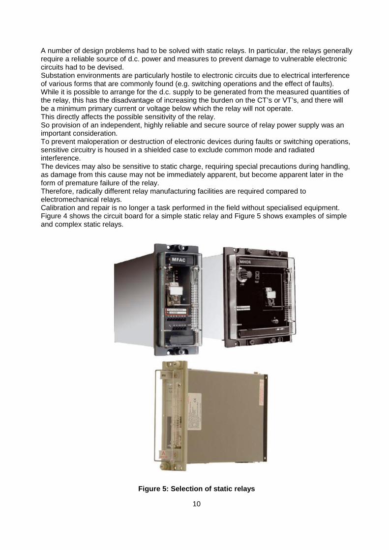
A number of design problems had to be solved with static relays. In particular, the relays generally require a reliable source of d.c. power and measures to prevent damage to vulnerable electronic circuits had to be devised. Substation environments are particularly hostile to electronic circuits due to electrical interference of various forms that are commonly found (e.g. switching operations and the effect of faults). While it is possible to arrange for the d.c. supply to be generated from the measured quantities of the relay, this has the disadvantage of increasing the burden on the CT’s or VT’s, and there will be a minimum primary current or voltage below which the relay will not operate. This directly affects the possible sensitivity of the relay. So provision of an independent, highly reliable and secure source of relay power supply was an important consideration. To prevent maloperation or destruction of electronic devices during faults or switching operations, sensitive circuitry is housed in a shielded case to exclude common mode and radiated interference. The devices may also be sensitive to static charge, requiring special precautions during handling, as damage from this cause may not be immediately apparent, but become apparent later in the form of premature failure of the relay. Therefore, radically different relay manufacturing facilities are required compared to electromechanical relays. Calibration and repair is no longer a task performed in the field without specialised equipment. Figure 4 shows the circuit board for a simple static relay and Figure 5 shows examples of simple and complex static relays.

Figure 5: Selection of static relays

11

Digital relays Digital protection relays introduced a step change in technology. Microprocessors and microcontrollers replaced analogue circuits used in static relays to implement relay functions. Early examples began to be introduced into service around 1980, and, with improvements in processing capacity, can still be regarded as current technology for many relay applications. However, such technology will be completely superseded within the next five years by numerical relays. Compared to static relays, digital relays introduce A/D conversion of all measured analogue quantities and use a microprocessor to implement the protection algorithm. The microprocessor may use some kind of counting technique, or use the Discrete Fourier Transform (DFT) to implement the algorithm. However, the typical microprocessors used have limited processing capacity and memory compared to that provided in numerical relays. The functionality tends therefore to be limited and restricted largely to the protection function itself. Additional functionality compared to that provided by an electromechanical or static relay is usually available, typically taking the form of a wider range of settings, and greater accuracy. A communications link to a remote computer may also be provided. The limited power of the microprocessors used in digital relays restricts the number of samples of the waveform that can be measured per cycle. This, in turn, limits the speed of operation of the relay in certain applications. Therefore, a digital relay for a particular protection function may have a longer operation time than the static relay equivalent. However, the extra time is not significant in terms of overall tripping time and possible effects of power system stability. Examples of digital relays are shown in Figure 6.

Figure 6: Selection of digital relays

12

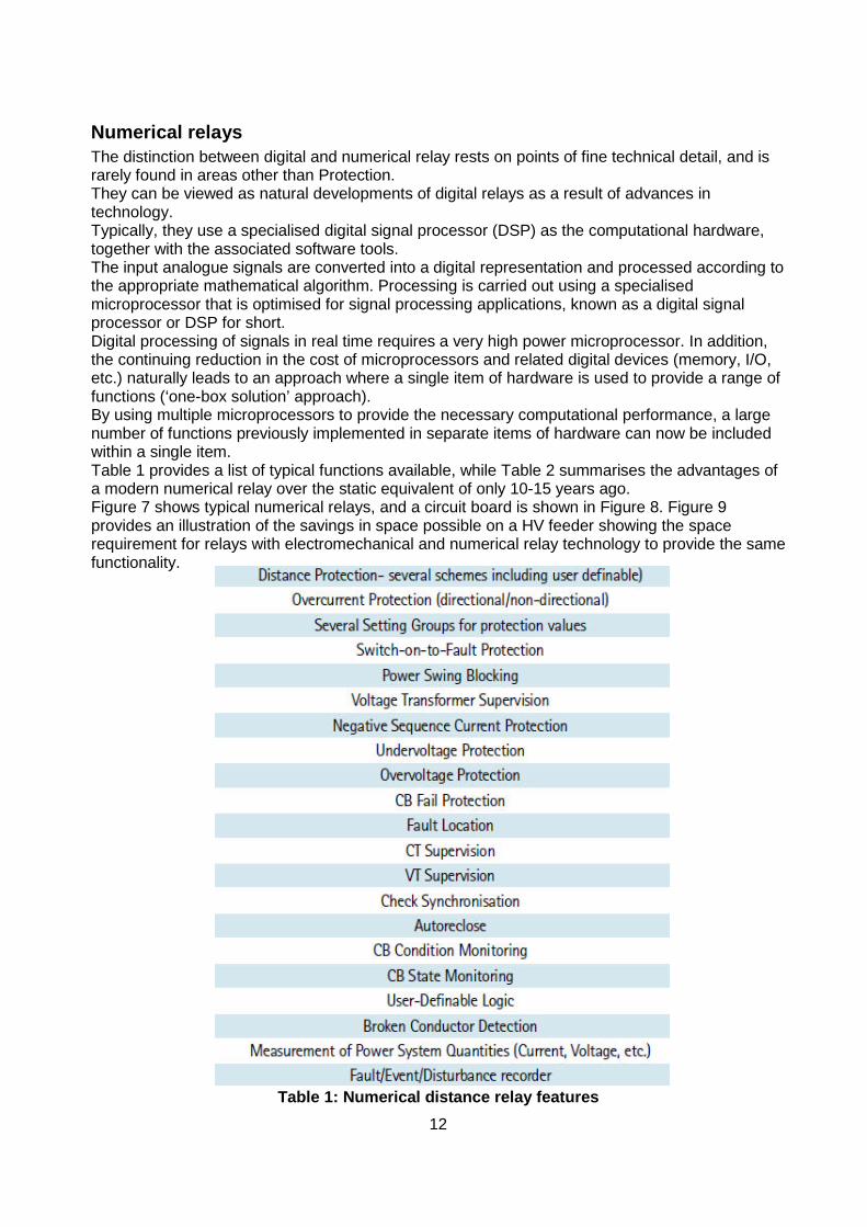
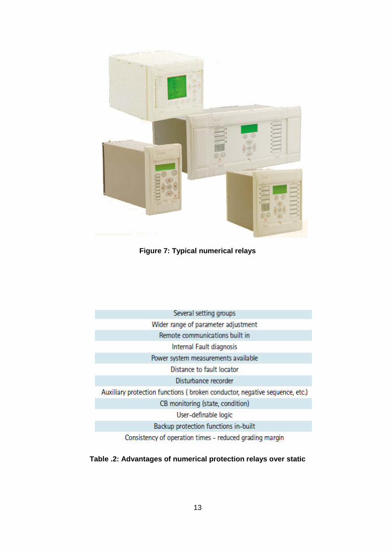
Numerical relays The distinction between digital and numerical relay rests on points of fine technical detail, and is rarely found in areas other than Protection. They can be viewed as natural developments of digital relays as a result of advances in technology. Typically, they use a specialised digital signal processor (DSP) as the computational hardware, together with the associated software tools. The input analogue signals are converted into a digital representation and processed according to the appropriate mathematical algorithm. Processing is carried out using a specialised microprocessor that is optimised for signal processing applications, known as a digital signal processor or DSP for short. Digital processing of signals in real time requires a very high power microprocessor. In addition, the continuing reduction in the cost of microprocessors and related digital devices (memory, I/O, etc.) naturally leads to an approach where a single item of hardware is used to provide a range of functions (‘one-box solution’ approach). By using multiple microprocessors to provide the necessary computational performance, a large number of functions previously implemented in separate items of hardware can now be included within a single item. Table 1 provides a list of typical functions available, while Table 2 summarises the advantages of a modern numerical relay over the static equivalent of only 10-15 years ago. Figure 7 shows typical numerical relays, and a circuit board is shown in Figure 8. Figure 9 provides an illustration of the savings in space possible on a HV feeder showing the space requirement for relays with electromechanical and numerical relay technology to provide the same functionality.

Table 1: Numerical distance relay features

13

Figure 7: Typical numerical relays

Table .2: Advantages of numerical protection relays over static

14

Because a numerical relay may implement the functionality that used to require several discrete relays, the relay functions (over-current, earth fault, etc.) are now referred to as being ‘relay elements’, so that a single relay (i.e. an item of hardware housed in a single case) may implement several functions using several relay elements. Each relay element will typically be a software routine or routines. The argument against putting many features into one piece of hardware centres on the issues of reliability and availability. A failure of a numerical relay may cause many more functions to be lost, compared to applications where different functions are implemented by separate hardware items. Comparison of reliability and availability between the two methods is complex as interdependency of elements of an application provided by separate relay elements needs to be taken into account. With the experience gained with static and digital relays, most hardware failure mechanisms are now well understood and suitable precautions taken at the design stage.

Figure 8: Circuit board for numerical relay Software problems are minimised by rigorous use of software design techniques, extensive prototype testing and the ability to download amended software into memory (possibly using a remote telephone link for download). Practical experience indicates that numerical relays are at least as reliable and have at least as good a record of availability as relays of earlier technologies. As the technology of numerical relays has only become available in recent years, a presentation of the concepts behind a numerical relay is presented in the following sections.

15

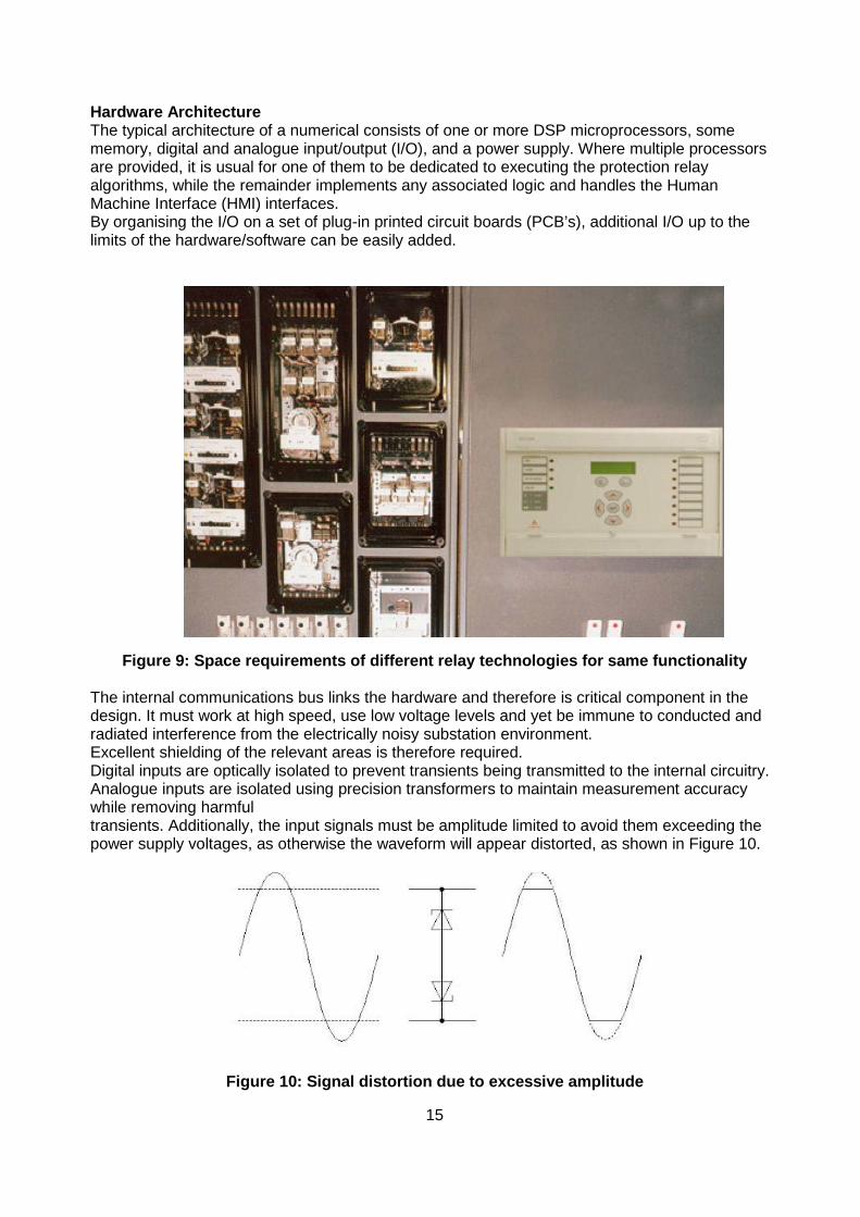
Hardware Architecture The typical architecture of a numerical consists of one or more DSP microprocessors, some memory, digital and analogue input/output (I/O), and a power supply. Where multiple processors are provided, it is usual for one of them to be dedicated to executing the protection relay algorithms, while the remainder implements any associated logic and handles the Human Machine Interface (HMI) interfaces. By organising the I/O on a set of plug-in printed circuit boards (PCB’s), additional I/O up to the limits of the hardware/software can be easily added.

Figure 9: Space requirements of different relay technologies for same functionality The internal communications bus links the hardware and therefore is critical component in the design. It must work at high speed, use low voltage levels and yet be immune to conducted and radiated interference from the electrically noisy substation environment. Excellent shielding of the relevant areas is therefore required. Digital inputs are optically isolated to prevent transients being transmitted to the internal circuitry. Analogue inputs are isolated using precision transformers to maintain measurement accuracy while removing harmful transients. Additionally, the input signals must be amplitude limited to avoid them exceeding the power supply voltages, as otherwise the waveform will appear distorted, as shown in Figure 10.

Figure 10: Signal distortion due to excessive amplitude

16

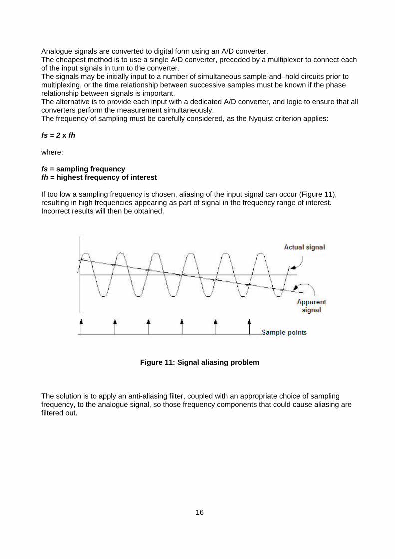
Analogue signals are converted to digital form using an A/D converter. The cheapest method is to use a single A/D converter, preceded by a multiplexer to connect each of the input signals in turn to the converter. The signals may be initially input to a number of simultaneous sample-and–hold circuits prior to multiplexing, or the time relationship between successive samples must be known if the phase relationship between signals is important. The alternative is to provide each input with a dedicated A/D converter, and logic to ensure that all converters perform the measurement simultaneously. The frequency of sampling must be carefully considered, as the Nyquist criterion applies: fs = 2 x fh where: fs = sampling frequency fh = highest frequency of interest If too low a sampling frequency is chosen, aliasing of the input signal can occur (Figure 11), resulting in high frequencies appearing as part of signal in the frequency range of interest. Incorrect results will then be obtained.

Figure 11: Signal aliasing problem

The solution is to apply an anti-aliasing filter, coupled with an appropriate choice of sampling frequency, to the analogue signal, so those frequency components that could cause aliasing are filtered out.

17

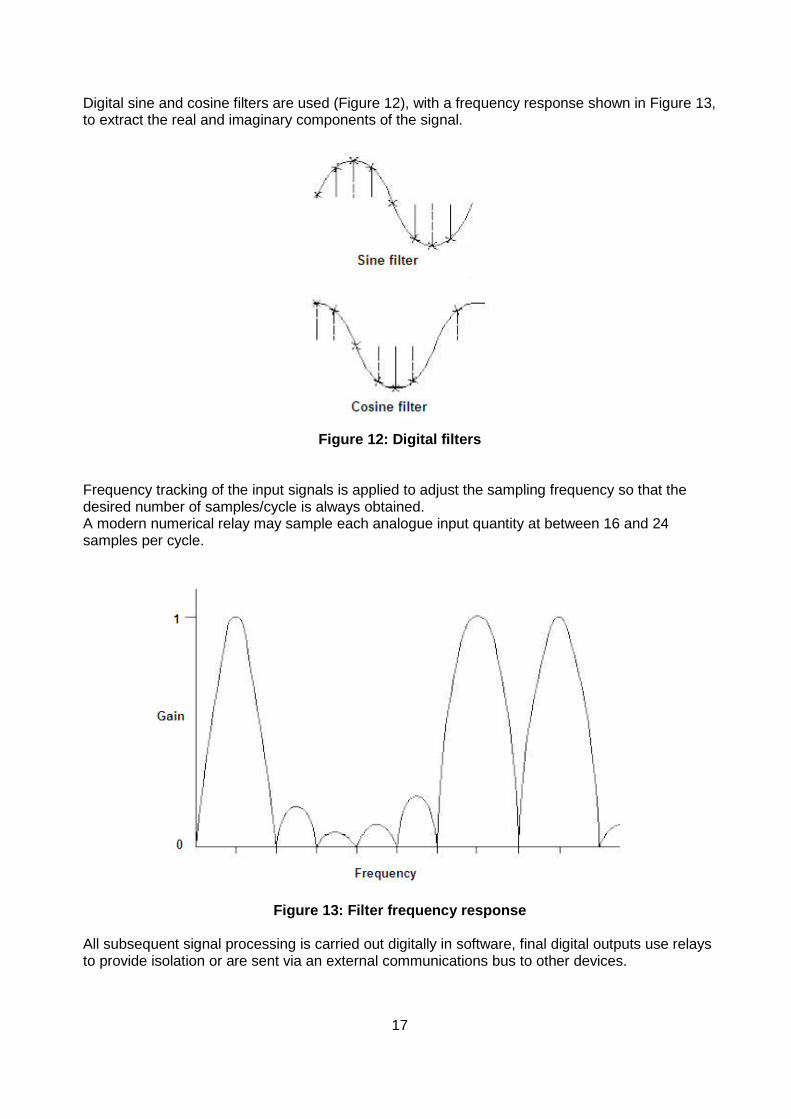
Digital sine and cosine filters are used (Figure 12), with a frequency response shown in Figure 13, to extract the real and imaginary components of the signal.

Figure 12: Digital filters Frequency tracking of the input signals is applied to adjust the sampling frequency so that the desired number of samples/cycle is always obtained. A modern numerical relay may sample each analogue input quantity at between 16 and 24 samples per cycle.

Figure 13: Filter frequency response All subsequent signal processing is carried out digitally in software, final digital outputs use relays to provide isolation or are sent via an external communications bus to other devices.

18

Relay Software The software provided is commonly organised into a series of tasks, operating in real time. An essential component is the Real Time Operating System (RTOS), whose function is to ensure that the other tasks are executed as and when required, on a priority basis. Other task software provided will naturally vary according to the function of the specific relay, but can be generalised as follows: a. system services software – this is akin to the BIOS of an ordinary PC, and controls the low-level I/O for the relay (i.e. drivers for the relay hardware, boot-up sequence, etc.) b. HMI interface software – the high level software for communicating with a user, via the front panel controls or through a data link to another computer running suitable software, storage of setting data, etc. c. application software – this is the software that defines the protection function of the relay d. auxiliary functions – software to implement other features offered in the relay – often structured as a series of modules to reflect the options offered to a user by the manufacturer Application Software The relevant software algorithm is then applied. Firstly, the values of the quantities of interest have to be determined from the available information contained in the data samples. This is conveniently done by the application of the Discrete Fourier Transform (DFT), and the result is magnitude and phase information for the selected quantity. This calculation is repeated for all of the quantities of interest. The quantities can then be compared with the relay characteristic, and a decision made in terms of the following: a. value above setting – start timers, etc. communications port, but some by their nature may only be available at one output interface. b. timer expired – action alarm/trip c. value returned below setting – reset timers, etc. d. value below setting – do nothing e. value still above setting – increment timer, etc. Since the overall cycle time for the software is known, timers are generally implemented as counters. Additional features of numerical relays The DSP chip in a numerical relay is normally of sufficient processing capacity that calculation of the relay protection function only occupies part of the processing capacity. The excess capacity is therefore available to perform other functions. Of course, care must be taken never to load the processor beyond capacity, for if this happens, the protection algorithm will not complete its calculation in the required time and the protection function will be compromised. Typical functions that may be found in a numerical relay besides protection functions are described in this section. Note that not all functions may be found in a particular relay. In common with earlier generations of relays, manufacturers, in accordance with their perceived market segmentation, will offer different versions offering a different set of functions. Function parameters will generally be available for display on the front panel of the relay.

19

Measured Values Display This is perhaps the most obvious and simple function to implement, as it involves the least additional processor time. The values that the relay must measure to perform its protection function have already been acquired and processed. It is therefore a simple task to display them on the front panel, and/or transmit as required to a remote computer/HMI station. Less obvious is that a number of extra quantities may be able to be derived from the measured quantities, depending on the input signals available. These might include: a. sequence quantities (positive, negative, zero) b. power, reactive power and power factor c. energy (kWh, kvarh) d. max. demand in a period (kW, kvar; average and peak values) e. harmonic quantities f. frequency g. temperatures/RTD status h. motor start information (start time, total no. of starts/reaccelerations, total running time i. distance to fault The accuracy of the measured values can only be as good as the accuracy of the transducers used (VT’s CT’s, A/D converter, etc.). As CT’s and VT’s for protection functions may have a different accuracy specification to those for metering functions, such data may not be sufficiently accurate for tariff purposes. However, it will be sufficiently accurate for an operator to assess system conditions and make appropriate decisions. VT/CT Supervision If suitable VT’s are used, supervision of the VT/CT supplies can be made available. VT supervision is made more complicated by the different conditions under which there may be no VT signal – some of which indicate VT failure and some occur because of a power system fault having occurred. CT supervision is carried out more easily, the general principle being the calculation of a level of negative sequence current that is inconsistent with the calculated value of negative sequence voltage. CB Control/State Indication /Condition Monitoring System operators will normally require knowledge of the state of all circuit breakers under their control. The CB position-switch outputs can be connected to the relay digital inputs and hence provide the indication of state via the communications bus to a remote control centre. Circuit breakers also require periodic maintenance of their operating mechanisms and contacts to ensure they will operate when required and that the fault capacity is not affected adversely. The requirement for maintenance is a function of the number of trip operations, the cumulative current broken and the type of breaker.

20

A numerical relay can record all of these parameters and hence be configured to send an alarm when maintenance is due. If maintenance is not carried out within defined criteria (such as a pre-defined time or number of trips) after maintenance is required, the CB can be arranged to trip and lockout, or inhibit certain functions such as auto-reclose. Finally, as well as tripping the CB as required under fault conditions, it can also be arranged for a digital output to be used for CB closure, so that separate CB close control circuits can be eliminated. Disturbance Recorder The relay memory requires a certain minimum number of cycles of measured data to be stored for correct signal processing and detection of events. The memory can easily be expanded to allow storage of a greater time period of input data, both analogue and digital, plus the state of the relay outputs. It then has the capability to act as a disturbance recorder for the circuit being monitored, so that by freezing the memory at the instant of fault detection or trip, a record of the disturbance is available for later download and analysis. It may be inconvenient to download the record immediately, so facilities may be provided to capture and store a number of disturbances. In industrial and small distribution networks, this may be all that is required. In transmission networks, it may be necessary to provide a single recorder to monitor a number of circuits simultaneously, and in this case, a separate disturbance recorder will still be required. Time Synchronisation Disturbance records and data relating to energyconsumption requires time tagging to serve any useful purpose. Although an internal clock will normally be present, this is of limited accuracy and use of this clock to provide time information may cause problems if the disturbance record has to be correlated with similar records from other sources to obtain a complete picture of an event. Many numerical relays have the facility for time synchronisation from an external clock. The standard normally used is an IRIG-B signal, which may be derived from a number of sources, the latest being from a GPS satellite system.

Programmable Logic Logic functions are well suited to implementation using microprocessors. The implementation of logic in a relay is not new, as functions such as intertripping and auto-reclose require a certain amount of logic. However, by providing a substantial number of digital I/O and making the logic capable of being programmed using suitable off-line software, the functionality of such schemes can be enhanced and/or additional features provided. For instance, an over-current relay at the receiving end of a transformer feeder could use the temperature inputs provided to monitor transformer winding temperature and provide alarm/trip facilities to the operator/upstream relay, eliminating the need for a separate winding temperature relay. This is an elementary example, but other advantages are evident to the relay manufacturer – different logic schemes required by different Utilities, etc., no longer need separate relay versions or some hard-wired logic to implement, reducing the cost of manufacture. It is also easier to customise a relay for a specific application, and eliminate other devices that would otherwise be required.

21

Provision of Setting Groups Historically, electromechanical and static relays have been provided with only one group of settings to be applied to the relay. Unfortunately, power systems change their topology due to operational reasons on a regular basis. (e.g. supply from normal/emergency generation). The different configurations may require different relay settings to maintain the desired level of network protection (since, for the above example, the fault levels will be significantly different on parts of the network that remain energised under both conditions). This problem can be overcome by the provision within the relay of a number of setting groups, only one of which is in use at any one time. Changeover between groups can be achieved from a remote command from the operator, or possibly through the programmable logic system. This may obviate the need for duplicate relays to be fitted with some form of switching arrangement of the inputs and outputs depending on network configuration. The operator will also have the ability to remotely program the relay with a group of settings if required.

Conclusions The provision of extra facilities in numerical relays may avoid the need for other measurement/control devices to be fitted in a substation. A trend can therefore be discerned in which protection relays are provided with functionality that in the past has been provided using separate equipment. The protection relay no longer performs a basic protection function; but is becoming an integral and major part of a substation automation scheme. The choice of a protection relay rather than some other device is logical, as the protection relay is probably the only device that is virtually mandatory on circuits of any significant rating. Thus, the functions previously carried out by separate devices such as bay controllers, discrete metering transducers and similar devices are now found in a protection relay. It is now possible to implement a substation automation scheme using numerical relays as the principal or indeed only hardware provided at bay level. As the power of microprocessors continues to grow and pressure on operators to reduce costs continues, this trend will probably continue, one obvious development being the provision of RTU facilities in designated relays that act as local concentrators of information within the overall network automation scheme.

Numerical relay issues The introduction of numerical relays replaces some of the issues of previous generations of relays with new ones. Some of the new issues that must be addressed are as follows: a. software version control b. relay data management c. testing and commissioning Software Version Control Numerical relays perform their functions by means of software. The process used for software generation is no different in principle to that for any other device using real-time software, and includes the difficulties of developing code that is error-free. Manufacturers must therefore pay particular attention to the methodology used for software generation and testing to ensure that as far as possible, the code contains no errors. However, it is virtually impossible to perform internal tests that cover all possible combinations of external effects, etc., and therefore it must be accepted that errors may exist.

22

In this respect, software used in relays is no different to any other software, where users accept that field use may uncover errors that may require changes to the software. Obviously, type testing can be expected to prove that the protection functions implemented by the relay are carried out properly, but it has been known for failures of rarely used auxiliary functions to occur under some conditions. Where problems are discovered in software subsequent to the release of a numerical relay for sale, a new version of the software may be considered necessary. This process then requires some form of software version control to be implemented to keep track of: a. the different software versions in existence b. the differences between each version c. the reasons for the change d. relays fitted with each of the versions With an effective version control system, manufacturers are able to advise users in the event of reported problems if the problem is a known software related problem and what remedial action is required. With the aid of suitable software held by a user, it may be possible to download the new software version instead of requiring a visit from a service engineer. Relay Data Management A numerical relay usually provides many more features than a relay using static or electromechanical technology. To use these features, the appropriate data must be entered into the memory of the relay. Users must also keep a record of all of the data, in case of data loss within the relay, or for use in system studies, etc. The amount of data per numerical relay may be 10-50 times that of an equivalent electromechanical relay, to which must be added the possibility of user-defined logic functions. The task of entering the data correctly into a numerical relay becomes a much more complex task than previously, which adds to the possibility of a mistake being made. Similarly, the amount of data that must be recorded is much larger, giving rise potentially to problems of storage. The problems have been addressed by the provision of software to automate the preparation and download of relay setting data from a portable computer connected to a communications port of the relay. As part of the process, the setting data can be read back from the relay and compared with the desired settings to ensure that the download has been error-free. A copy of the setting data (including user defined logic schemes where used) can also be stored on the computer, for later printout and/or upload to the users database facilities. More advanced software is available to perform the above functions from an Engineering Computer in a substation automation scheme. Relay Testing and Commissioning The testing of relays based on software is of necessity radically different from earlier generations of relays. Site commissioning is usually restricted to the in-built software self-check and verification that currents and voltages measured by the relay are correct. Problems revealed by such tests require specialist equipment to resolve, and hence field policy is usually on a repair-by-replacement basis.

23

24

Transformers A transformer is a device that transfers electrical energy from one circuit to another through inductively coupled conductors — the transformer's coils. A varying current in the first or primary winding creates a varying magnetic field through the secondary winding. This varying magnetic field induces a varying electromotive force (EMF) or "voltage" in the "secondary" winding. This effect is called mutual induction. If a load is connected to the secondary, an electric current will flow in the secondary winding and electrical energy will be transferred from the primary circuit through the transformer to the load. In an ideal transformer, the induced voltage in the secondary winding (VS) is in proportion to the primary voltage (VP), and is given by the ratio of the number of turns in the secondary (NS) to the number of turns in the primary (NP) as follows:

By appropriate selection of the ratio of turns, a transformer thus allows an alternating current (AC) voltage to be "stepped up" by making NS greater than NP, or "stepped down" by making NS less than NP. In the vast majority of transformers, the coils are wound around a ferromagnetic core, air-core transformers being a notable exception. Transformers come in a range of sizes from a thumbnail-sized coupling transformer hidden inside a stage microphone to huge units weighing hundreds of tons used to interconnect portions of national power grids.

Pole-mounted single-phase transformer with center-tapped secondary All operate with the same basic principles, although the range of designs is wide. While new technologies have eliminated the need for transformers in some electronic circuits, transformers are still found in nearly all electronic devices designed for household ("mains") voltage. Transformers are essential for high voltage power transmission, which makes long distance transmission economically practical.

25

Basic principles The transformer is based on two principles: firstly, that an electric current can produce a magnetic field (electromagnetism) and secondly that a changing magnetic field within a coil of wire induces a voltage across the ends of the coil (electromagnetic induction). Changing the current in the primary coil changes the magnetic flux that is developed. The changing magnetic flux induces a voltage in the secondary coil. An ideal transformer is shown in the diagram below

Current passing through the primary coil creates a magnetic field. The primary and secondary coils are wrapped around a core of very high magnetic permeability, such as iron, so that most of the magnetic flux passes through both primary and secondary coils. Induction law The voltage induced across the secondary coil may be calculated from Faraday's law of induction, which states that:

where VS is the instantaneous voltage, NS is the number of turns in the secondary coil and Φ equals the magnetic flux through one turn of the coil. If the turns of the coil are oriented perpendicular to the magnetic field lines, the flux is the product of the magnetic field strength B and the area A through which it cuts. The area is constant, being equal to the cross-sectional area of the transformer core, whereas the magnetic field varies with time according to the excitation of the primary. Since the same magnetic flux passes through both the primary and secondary coils in an ideal transformer, the instantaneous voltage across the primary winding equals

Taking the ratio of the two equations for VS and VP gives the basic equation for stepping up or stepping down the voltage

26

Ideal power equation If the secondary coil is attached to a load that allows current to flow, electrical power is transmitted from the primary circuit to the secondary circuit. Ideally, the transformer is perfectly efficient; all the incoming energy is transformed from the primary circuit to the magnetic field and into the secondary circuit. If this condition is met, the incoming electric power must equal the outgoing power. P incoming = IPVP = P outgoing = ISVS giving the ideal transformer equation

Transformers are efficient so this formula is a reasonable approximation. If the voltage is increased, then the current is decreased by the same factor. The impedance in one circuit is transformed by the square of the turns ratio. For example, if an impedance ZS is attached across the terminals of the secondary coil, it appears to the primary circuit to have an impedance of . This relationship is reciprocal, so that the impedance ZP of the primary circuit appears to the secondary to be .

The ideal transformer as a circuit element

Detailed operation The simplified description above neglects several practical factors, in particular the primary current required to establish a magnetic field in the core, and the contribution to the field due to current in the secondary circuit. Models of an ideal transformer typically assume a core of negligible reluctance with two windings of zero resistance. When a voltage is applied to the primary winding, a small current flows, driving flux around the magnetic circuit of the core. The current required to create the flux is termed the magnetizing current; since the ideal core has been assumed to have near-zero reluctance, the magnetizing current is negligible, although still required to create the magnetic field. The changing magnetic field induces an electromotive force (EMF) across each winding. Since the ideal windings have no impedance, they have no associated voltage drop, and so the voltages VP and VS measured at the terminals of the transformer, are equal to the corresponding EMFs. The primary EMF, acting as it does in opposition to the primary voltage, is sometimes termed the "back EMF". This is due to Lenz's law which states that the induction of EMF would always be such that it will oppose development of any such change in magnetic field.

27

Practical considerations Leakage flux The ideal transformer model assumes that all flux generated by the primary winding links all the turns of every winding, including itself. In practice, some flux traverses paths that take it outside the windings. Such flux is termed leakage flux, and results in leakage inductance in series with the mutually coupled transformer windings.

Leakage flux of a transformer Leakage results in energy being alternately stored in and discharged from the magnetic fields with each cycle of the power supply. It is not directly a power loss (see "Stray losses" below), but results in inferior voltage regulation, causing the secondary voltage to fail to be directly proportional to the primary, particularly under heavy load. Transformers are therefore normally designed to have very low leakage inductance. However, in some applications, leakage can be a desirable property, and long magnetic paths, air gaps, or magnetic bypass shunts may be deliberately introduced to a transformer's design to limit the short-circuit current it will supply. Leaky transformers may be used to supply loads that exhibit negative resistance, such as electric arcs, mercury vapor lamps, and neon signs; or for safely handling loads that become periodically short-circuited such as electric arc welders. Air gaps are also used to keep a transformer from saturating, especially audio-frequency transformers in circuits that have a direct current flowing through the windings.

Effect of frequency If the flux in the core is sinusoidal, the relationship for either winding between its rms Voltage of the winding E, and the supply frequency f, number of turns N, core cross-sectional area a and peak magnetic flux density B is given by the universal EMF equation:

Transformer universal EMF equation The time-derivative term in Faraday's Law shows that the flux in the core is the integral of the applied voltage.

28

Hypothetically an ideal transformer would work with direct-current excitation, with the core flux increasing linearly with time. In practice, the flux would rise to the point where magnetic saturation of the core occurs, causing a huge increase in the magnetizing current and overheating the transformer. All practical transformers must therefore operate with alternating (or pulsed) current The EMF of a transformer at a given flux density increases with frequency. By operating at higher frequencies, transformers can be physically more compact because a given core is able to transfer more power without reaching saturation, and fewer turns are needed to achieve the same impedance. However properties such as core loss and conductor skin effect also increase with frequency. Aircraft and military equipment employ 400 Hz power supplies which reduce core and winding weight. Operation of a transformer at its designed voltage but at a higher frequency than intended will lead to reduced magnetizing current; at lower frequency, the magnetizing current will increase. Operation of a transformer at other than its design frequency may require assessment of voltages, losses, and cooling to establish if safe operation is practical. For example, transformers may need to be equipped with "volts per hertz" over-excitation relays to protect the transformer from overvoltage at higher than rated frequency. Knowledge of natural frequencies of transformer windings is of importance for the determination of the transient response of the windings to impulse and switching surge voltages.

Energy losses An ideal transformer would have no energy losses, and would be 100% efficient. In practical transformers energy is dissipated in the windings, core, and surrounding structures. Larger transformers are generally more efficient, and those rated for electricity distribution usually perform better than 98%. Experimental transformers using superconducting windings achieve efficiencies of 99.85%, While the increase in efficiency is small, when applied to large heavily-loaded transformers the annual savings in energy losses are significant. A small transformer, such as a plug-in "wall-wart" or power adapter type used for low-power consumer electronics, may be no more than 85% efficient, with considerable loss even when not supplying any load. Though individual power loss is small, the aggregate losses from the very large number of such devices is coming under increased scrutiny. The losses vary with load current, and may be expressed as "no-load" or "full-load" loss. Winding resistance dominates load losses, whereas hysteresis and eddy currents losses contribute to over 99% of the no-load loss. The no-load loss can be significant, meaning that even an idle transformer constitutes a drain on an electrical supply, which encourages development of low-loss transformers Transformer losses are divided into losses in the windings, termed copper loss, and those in the magnetic circuit, termed iron loss. Losses in the transformer arise from: Winding resistance Current flowing through the windings causes resistive heating of the conductors. At higher frequencies, skin effect and proximity effect create additional winding resistance and losses. Hysteresis losses Each time the magnetic field is reversed, a small amount of energy is lost due to hysteresis within the core. For a given core material, the loss is proportional to the frequency, and is a function of the peak flux density to which it is subjected.

29

Eddy currents Ferromagnetic materials are also good conductors, and a solid core made from such a material also constitutes a single short-circuited turn throughout its entire length. Eddy currents therefore circulate within the core in a plane normal to the flux, and are responsible for resistive heating of the core material. The eddy current loss is a complex function of the square of supply frequency and inverse square of the material thickness. Magnetostriction Magnetic flux in a ferromagnetic material, such as the core, causes it to physically expand and contract slightly with each cycle of the magnetic field, an effect known as magnetostriction. This produces the buzzing sound commonly associated with transformers, and in turn causes losses due to frictional heating in susceptible cores. Mechanical losses In addition to magnetostriction, the alternating magnetic field causes fluctuating electromagnetic forces between the primary and secondary windings. These incite vibrations within nearby metalwork, adding to the buzzing noise, and consuming a small amount of power. Stray losses Leakage inductance is by itself lossless, since energy supplied to its magnetic fields is returned to the supply with the next half-cycle. However, any leakage flux that intercepts nearby conductive materials such as the transformer's support structure will give rise to eddy currents and be converted to heat.

Dot Convention It is common in transformer schematic symbols for there to be a dot at the end of each coil within a transformer, particularly for transformers with multiple windings on either or both of the primary and secondary sides. The purpose of the dots is to indicate the direction of each winding relative to the other windings in the transformer. Voltages at the dot end of each winding are in phase, while current flowing into the dot end of a primary coil will result in current flowing out of the dot end of a secondary coil.

30

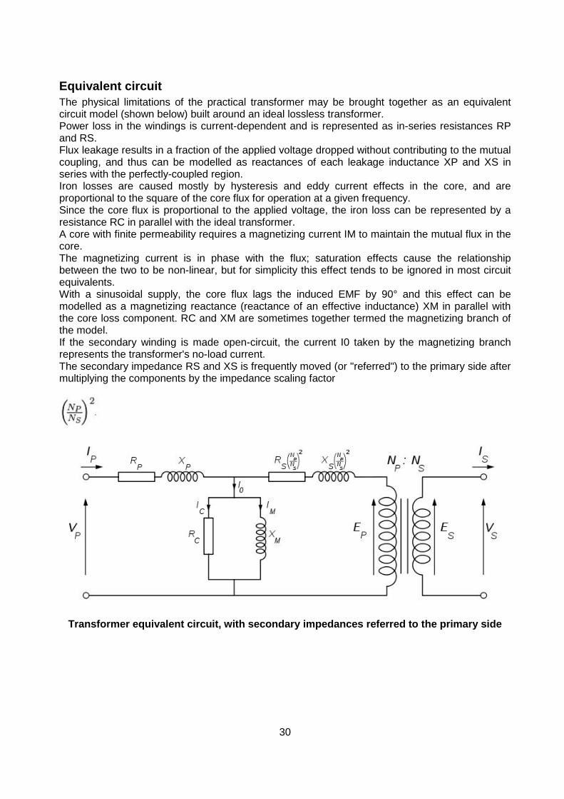
Equivalent circuit The physical limitations of the practical transformer may be brought together as an equivalent circuit model (shown below) built around an ideal lossless transformer. Power loss in the windings is current-dependent and is represented as in-series resistances RP and RS. Flux leakage results in a fraction of the applied voltage dropped without contributing to the mutual coupling, and thus can be modelled as reactances of each leakage inductance XP and XS in series with the perfectly-coupled region. Iron losses are caused mostly by hysteresis and eddy current effects in the core, and are proportional to the square of the core flux for operation at a given frequency. Since the core flux is proportional to the applied voltage, the iron loss can be represented by a resistance RC in parallel with the ideal transformer. A core with finite permeability requires a magnetizing current IM to maintain the mutual flux in the core. The magnetizing current is in phase with the flux; saturation effects cause the relationship between the two to be non-linear, but for simplicity this effect tends to be ignored in most circuit equivalents. With a sinusoidal supply, the core flux lags the induced EMF by 90° and this effect can be modelled as a magnetizing reactance (reactance of an effective inductance) XM in parallel with the core loss component. RC and XM are sometimes together termed the magnetizing branch of the model. If the secondary winding is made open-circuit, the current I0 taken by the magnetizing branch represents the transformer's no-load current. The secondary impedance RS and XS is frequently moved (or "referred") to the primary side after multiplying the components by the impedance scaling factor

Transformer equivalent circuit, with secondary impedances referred to the primary side

31

Types A wide variety of transformer designs are used for different applications, though they share several common features. Important common transformer types include: Autotransformer

An autotransformer with a sliding brush contact

An autotransformer has only a single winding with two end terminals, plus a third at an intermediate tap point. The primary voltage is applied across two of the terminals, and the secondary voltage taken from one of these and the third terminal. The primary and secondary circuits therefore have a number of windings turns in common. Since the volts-per-turn is the same in both windings, each develops a voltage in proportion to its number of turns. An adjustable autotransformer is made by exposing part of the winding coils and making the secondary connection through a sliding brush, giving a variable turns ratio. Such a device is often referred to as a variac.

Polyphase transformers.

Three-phase step-down transformer mounted between two utility poles.

32

For three-phase supplies, a bank of three individual single-phase transformers can be used, or all three phases can be incorporated as a single three-phase transformer. In this case, the magnetic circuits are connected together, the core thus containing a three-phase flow of flux. A number of winding configurations are possible, giving rise to different attributes and phase shifts. One particular polyphase configuration is the zigzag transformer, used for grounding and in the suppression of harmonic currents.

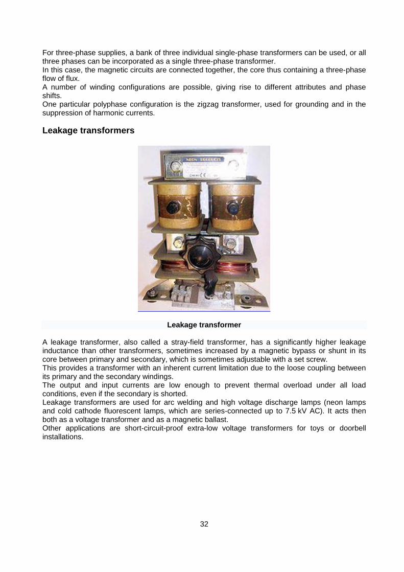
Leakage transformers

Leakage transformer A leakage transformer, also called a stray-field transformer, has a significantly higher leakage inductance than other transformers, sometimes increased by a magnetic bypass or shunt in its core between primary and secondary, which is sometimes adjustable with a set screw. This provides a transformer with an inherent current limitation due to the loose coupling between its primary and the secondary windings. The output and input currents are low enough to prevent thermal overload under all load conditions, even if the secondary is shorted. Leakage transformers are used for arc welding and high voltage discharge lamps (neon lamps and cold cathode fluorescent lamps, which are series-connected up to 7.5 kV AC). It acts then both as a voltage transformer and as a magnetic ballast. Other applications are short-circuit-proof extra-low voltage transformers for toys or doorbell installations.

33

Resonant transformers A resonant transformer is a kind of the leakage transformer. It uses the leakage inductance of its secondary windings in combination with external capacitors, to create one or more resonant circuits. Resonant transformers such as the Tesla coil can generate very high voltages, and are able to provide much higher current than electrostatic high-voltage generation machines such as the Van de Graaff generator. One of the applications of the resonant transformer is for the CCFL inverter. Another application of the resonant transformer is to couple between stages of a superheterodyne receiver, where the selectivity of the receiver is provided by tuned transformers in the intermediate-frequency amplifiers.

Audio transformers Audio transformers are those specifically designed for use in audio circuits. They can be used to block radio frequency interference or the DC component of an audio signal, to split or combine audio signals, or to provide impedance matching between high and low impedance circuits, such as between a high impedance tube (valve) amplifier output and a low impedance loudspeaker, or between a high impedance instrument output and the low impedance input of a mixing console. Such transformers were originally designed to connect different telephone systems to one another while keeping their respective power supplies isolated, and are still commonly used to interconnect professional audio systems or system components. Being magnetic devices, audio transformers are susceptible to external magnetic fields such as those generated by AC current-carrying conductors. "Hum" is a term commonly used to describe unwanted signals originating from the "mains" power supply (typically 50 or 60 Hz). Audio transformers used for low-level signals, such as those from microphones, often included shielding to protect against extraneous magnetically-coupled signals.

Instrument transformers Instrument transformers are used for measuring voltage and current in electrical power systems, and for power system protection and control. where a voltage or current is too large to be conveniently used by an instrument, it can be scaled down to a standardized, low value. Instrument transformers isolate measurement, protection and control circuitry from the high currents or voltages present on the circuits being measured or controlled.

Current transformers, designed for placing around conductors A current transformer is a transformer designed to provide a current in its secondary coil proportional to the current flowing in its primary coil.

34

Voltage transformers (VTs), also referred to as "potential transformers" (PTs), are designed to have an accurately-known transformation ratio in both magnitude and phase, over a range of measuring circuit impedances. A voltage transformer is intended to present a negligible load to the supply being measured. The low secondary voltage allows protective relay equipment and measuring instruments to be operated at a lower voltages. Both current and voltage instrument transformers are designed to have predictable characteristics on overloads. Proper operation of over-current protection relays requires that current transformers provide a predictable transformation ratio even during a short-circuit.

Current and Voltage Transformers

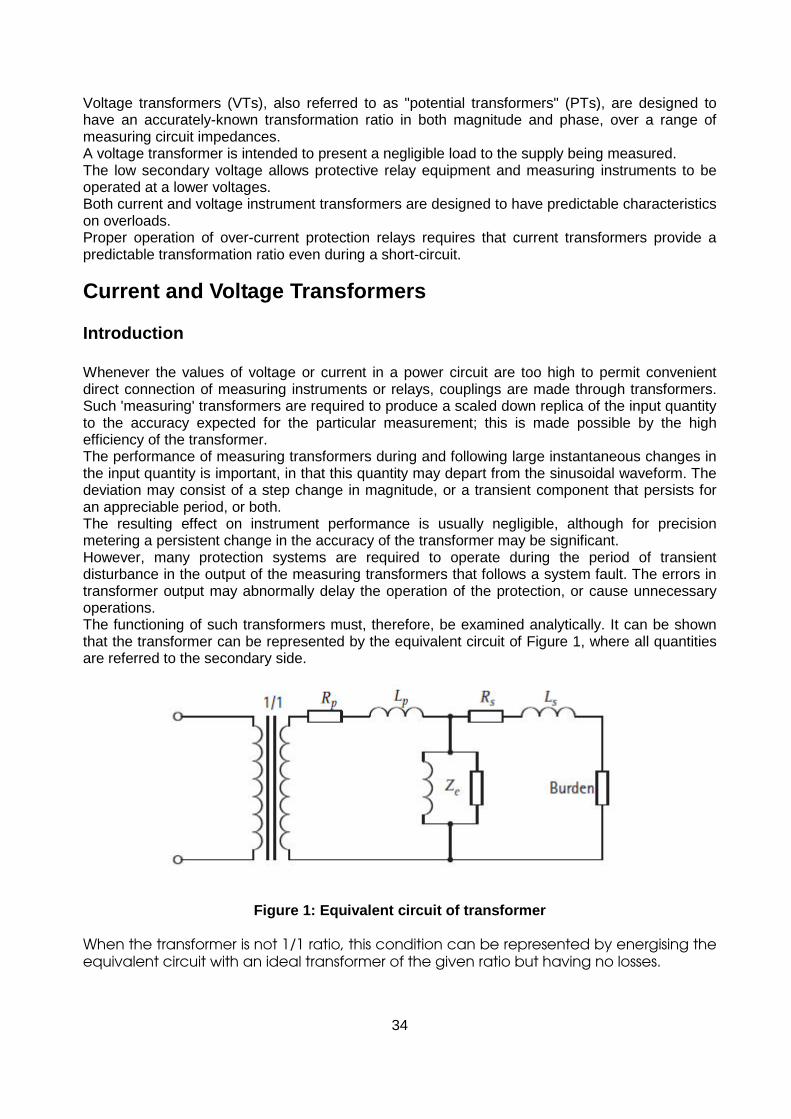
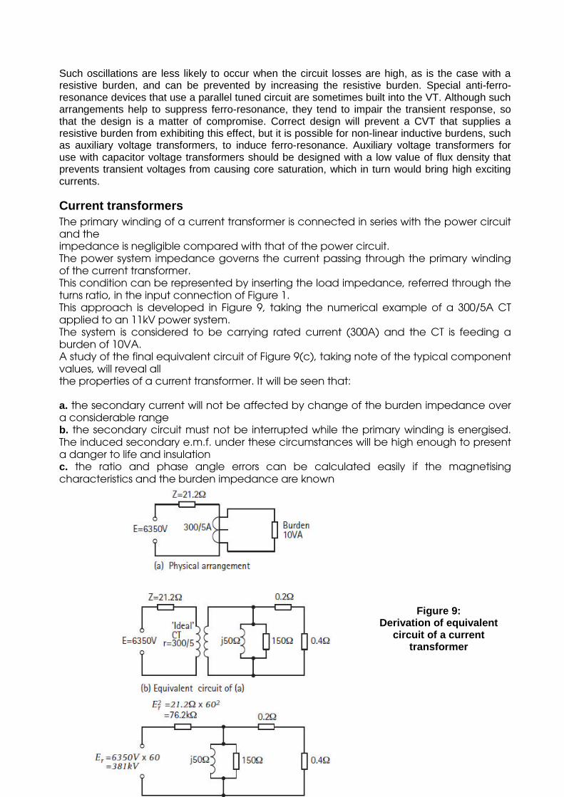
Introduction Whenever the values of voltage or current in a power circuit are too high to permit convenient direct connection of measuring instruments or relays, couplings are made through transformers. Such 'measuring' transformers are required to produce a scaled down replica of the input quantity to the accuracy expected for the particular measurement; this is made possible by the high efficiency of the transformer. The performance of measuring transformers during and following large instantaneous changes in the input quantity is important, in that this quantity may depart from the sinusoidal waveform. The deviation may consist of a step change in magnitude, or a transient component that persists for an appreciable period, or both. The resulting effect on instrument performance is usually negligible, although for precision metering a persistent change in the accuracy of the transformer may be significant. However, many protection systems are required to operate during the period of transient disturbance in the output of the measuring transformers that follows a system fault. The errors in transformer output may abnormally delay the operation of the protection, or cause unnecessary operations. The functioning of such transformers must, therefore, be examined analytically. It can be shown that the transformer can be represented by the equivalent circuit of Figure 1, where all quantities are referred to the secondary side.

Figure 1: Equivalent circuit of transformer

When the transformer is not 1/1 ratio, this condition can be represented by energising the equivalent circuit with an ideal transformer of the given ratio but having no losses.

35

Measuring Transformers Voltage and current transformers for low primary voltage or current ratings are not readily distinguishable; for higher ratings, dissimilarities of construction are usual. Nevertheless the differences between these devices lie principally in the way they are connected into the power circuit. Voltage transformers are much like small power transformers, differing only in details of design that control ratio accuracy over the specified range of output. Current transformers have their primary windings connected in series with the power circuit, and so also in series with the system impedance. The response of the transformer is radically different in these two modes of operation.

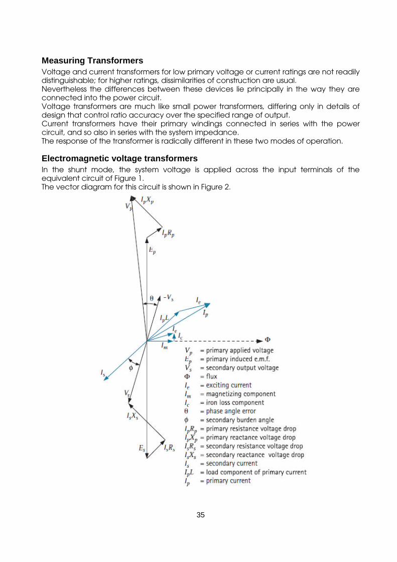
Electromagnetic voltage transformers In the shunt mode, the system voltage is applied across the input terminals of the equivalent circuit of Figure 1. The vector diagram for this circuit is shown in Figure 2.

36

Figure 2: Vector diagram for voltage transformer The secondary output voltage Vs is required to be an accurate scaled replica of the input voltage Vp over a specified range of output. To this end, the windingvoltage drops are made small, and the normal flux density in the core is designed to be well below the saturation density, in order that the exciting current may be low and the exciting impedance substantially constant with a variation of applied voltage over the desired operating range including some degree of overvoltage. These limitations in design result in a VT for a given burden being much larger than a typical power transformer of similar rating. The exciting current, in consequence, will not be as small, relative to the rated burden, as it would be for a typical power transformer. Errors The ratio and phase errors of the transformer can be calculated using the vector diagram of Figure 2. The ratio error is defined as:

where: Kn is the nominal ratio Vp is the primary voltage Vs is the secondary voltage If the error is positive, the secondary voltage exceeds the nominal value. The turns ratio of the transformer need not be equal to the nominal ratio; a small turns compensation will usually be employed, so that the error will be positive for low burdens and negative for high burdens. The phase error is the phase difference between the reversed secondary and the primary voltage vectors. It is positive when the reversed secondary voltage leads the primary vector. Requirements in this respect are set out in IEC 60044-2. All voltage transformers are required to comply with one of the classes in Table 1. For protection purposes, accuracy of voltage measurement may be important during fault conditions, as the system voltage might be reduced by the fault to a low value. Voltage transformers for such types of service must comply with the extended range of requirements set out in Table 2.

Table 1: Measuring voltage transformer error limits

37

Table.2: Additional limits for protection voltage transformers Voltage Factors The quantity Vf in Table 2 is an upper limit of operating voltage, expressed in per unit of rated voltage. This is important for correct relay operation and operation under unbalanced fault conditions on unearthed or impedance earthed systems, resulting in a rise in the voltage on the healthy phases. Voltage factors, with the permissible duration of the maximum voltage, are given in Table 3.

Table.3: Voltage transformers: Permissible duration of maximum voltage

Secondary Leads Voltage transformers are designed to maintain the specified accuracy in voltage output at their secondary terminals. To maintain this if long secondary leads are required, a distribution box can be fitted close to the VT to supply relay and metering burdens over separate leads. If necessary, allowance can be made for the resistance of the leads to individual burdens when the particular equipment is calibrated.

38

Protection of Voltage Transformers Voltage Transformers can be protected by H.R.C. fuses on the primary side for voltages up to 66kV. Fuses do not usually have a sufficient interrupting capacity for use with higher voltages. Practice varies, and in some cases protection on the primary is omitted. The secondary of a Voltage Transformer should always be protected by fuses or a miniature circuit breaker (MCB). The device should be located as near to the transformer as possible. A short circuit on the secondary circuit wiring will produce a current of many times the rated output and cause excessive heating. Even where primary fuses can be fitted, these will usually not clear a secondary side short circuit because of the low value of primary current and the minimum practicable fuse rating. Construction The construction of a voltage transformer takes into account the following factors: a. output – seldom more than 200-300VA. Cooling is rarely a problem b. insulation – designed for the system impulsevoltage level. Insulation volume is often largerthan the winding volume c. mechanical design – not usually necessary to withstand short-circuit currents. Must be small to fit the space available within switchgear Three-phase units are common up to 36kV but for higher voltages single-phase units are usual. Voltage transformers for medium voltage circuits will have dry type insulation, but for high and extra high voltage systems, oil immersed units are general. Resin encapsulated designs are in use on systems up to 33kV. Figure 3 shows a typical voltage transformer.

Figure 3: Typical voltage transformer

39

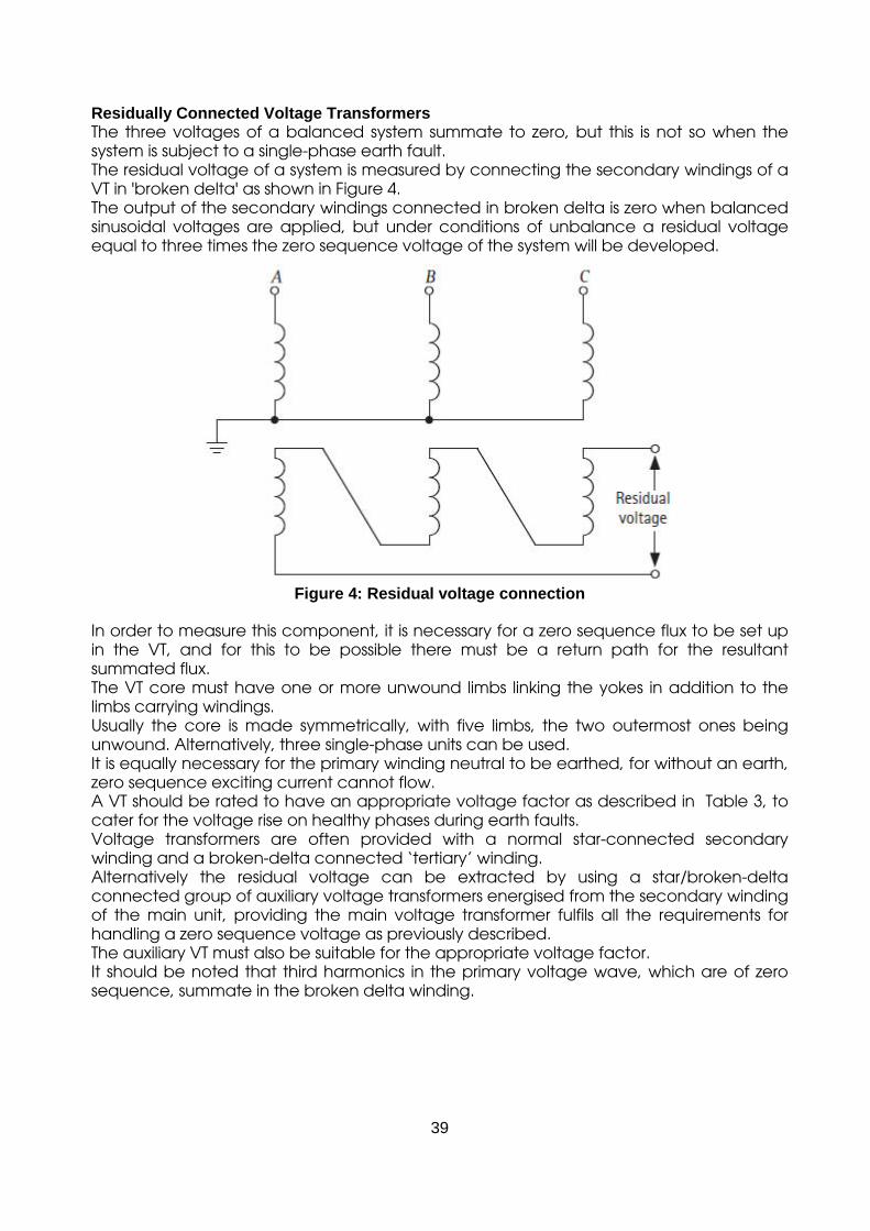
Residually Connected Voltage Transformers The three voltages of a balanced system summate to zero, but this is not so when the system is subject to a single-phase earth fault. The residual voltage of a system is measured by connecting the secondary windings of a VT in 'broken delta' as shown in Figure 4. The output of the secondary windings connected in broken delta is zero when balanced sinusoidal voltages are applied, but under conditions of unbalance a residual voltage equal to three times the zero sequence voltage of the system will be developed.

Figure 4: Residual voltage connection

In order to measure this component, it is necessary for a zero sequence flux to be set up in the VT, and for this to be possible there must be a return path for the resultant summated flux. The VT core must have one or more unwound limbs linking the yokes in addition to the limbs carrying windings. Usually the core is made symmetrically, with five limbs, the two outermost ones being unwound. Alternatively, three single-phase units can be used. It is equally necessary for the primary winding neutral to be earthed, for without an earth, zero sequence exciting current cannot flow. A VT should be rated to have an appropriate voltage factor as described in Table 3, to cater for the voltage rise on healthy phases during earth faults. Voltage transformers are often provided with a normal star-connected secondary winding and a broken-delta connected ‘tertiary’ winding. Alternatively the residual voltage can be extracted by using a star/broken-delta connected group of auxiliary voltage transformers energised from the secondary winding of the main unit, providing the main voltage transformer fulfils all the requirements for handling a zero sequence voltage as previously described. The auxiliary VT must also be suitable for the appropriate voltage factor. It should be noted that third harmonics in the primary voltage wave, which are of zero sequence, summate in the broken delta winding.

40

Transient Performance Transient errors cause few difficulties in the use of conventional voltage transformers although some do occur. Errors are generally limited to short time periods following the sudden application or removal of voltage from the VT primary. If a voltage is suddenly applied, an inrush transient will occur, as with power transformers. The effect will, however, be less severe than for power transformers because of the lower flux density for which the VT is designed. If the VT is rated to have a fairly high voltage factor, little inrush effect will occur. An error will appear in the first few cycles of the output current in proportion to the inrush transient that occurs. When the supply to a voltage transformer is interrupted, the core flux will not readily collapse; the secondary winding will tend to maintain the magnetising force to sustain this flux, and will circulate a current through the burden which will decay more or less exponentially, possible with a superimposed audio-frequency oscillation due to the capacitance of the winding. Bearing in mind that the exciting quantity, expressed in ampere-turns, may exceed the burden, the transient current may be significant. Cascade Voltage Transformers The capacitor VT was developed because of the high cost of conventional electromagnetic voltage transformers but, the frequency and transient responses are less satisfactory than those of the orthodox voltage transformers. Another solution to the problem is the cascade VT (Figure 5).

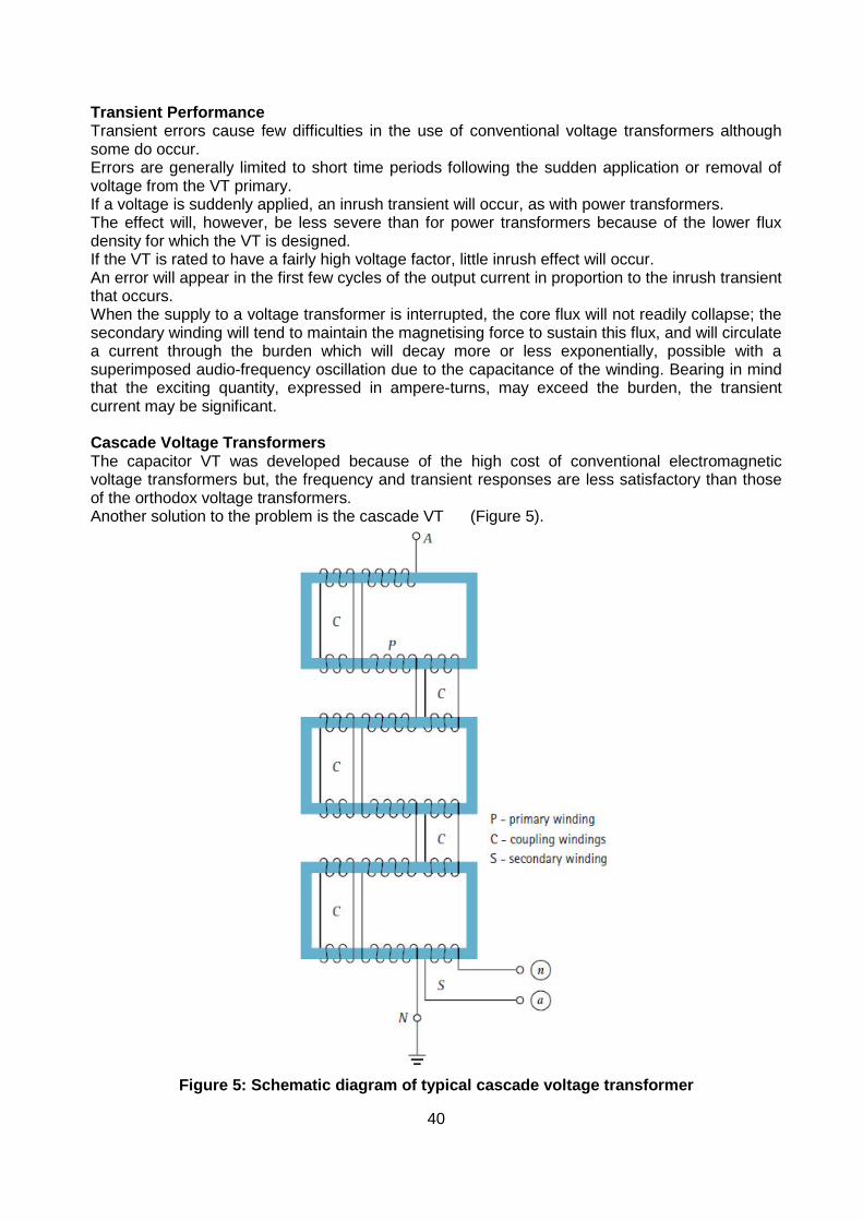
Figure 5: Schematic diagram of typical cascade voltage transformer

41

The conventional type of VT has a single primary winding, the insulation of which presents a great problem for voltages above about 132kV. The cascade VT avoids these difficulties by breaking down the primary voltage in several distinct and separate stages. The complete VT is made up of several individual transformers, the primary windings of which are connected in series, as shown in Figure 5. Each magnetic core has primary windings (P) on two opposite sides. The secondary winding (S) consists of a single winding on the last stage only. Coupling windings (C) connected in pairs between stages, provide low impedance circuits for the transfer of load ampere-turns between stages and ensure that the power frequency voltage is equally distributed over the several primary windings. The potentials of the cores and coupling windings are fixed at definite values by connecting them to selected points on the primary windings. The insulation of each winding is sufficient for the voltage developed in that winding, which is a fraction of the total according to the number of stages. The individual transformers are mounted on a structure built of insulating material, which provides the interstage insulation, accumulating to a value able to withstand the full system voltage across the complete height of the stack. The entire assembly is contained in a hollow cylindrical porcelain housing with external weather-sheds; the housing is filled with oil and sealed, an expansion bellows being included to maintain hermetic sealing and to permit expansion with temperature change.

Capacitor voltage transformers The size of electromagnetic voltage transformers for the higher voltages is largely proportional to the rated voltage; the cost tends to increase at a disproportionate rate. The capacitor voltage transformer (CVT) is often more economic. This device is basically a capacitance potential divider. As with resistance-type potential dividers, the output voltage is seriously affected by load at the tapping point. The capacitance divider differs in that its equivalent source impedance is capacitive and can therefore be compensated by a reactor connected in series with the tapping point. With an ideal reactor, such an arrangement would have no regulation and could supply any value of output. A reactor possesses some resistance, which limits the output that can be obtained. For a secondary output voltage of 110V, the capacitors would have to be very large to provide a useful output while keeping errors within the usual limits. The solution is to use a high secondary voltage and further transform the output to the normal value using a relatively inexpensive electromagnetic transformer. The successive stages of this reasoning are indicated in Figure 6.

Figure 6 Development of capacitor voltage transformer

42

There are numerous variations of this basic circuit. The inductance L may be a separate unit or it may be incorporated in the form of leakage reactance in the transformer T. Capacitors C1 and C2 cannot conveniently be made to close tolerances, so tappings are provided for ratio adjustment, either on the transformer T, or on a separate auto-transformer in the secondary circuit. Adjustment of the tuning inductance L is also needed; this can be done with tappings, a separate tapped inductor in the secondary circuit, by adjustment of gaps in the iron cores, or by shunting with variable capacitance. A simplified equivalent circuit is shown in Figure 7.

Figure 7: Simplified equivalent circuit of capacitor voltage transformer

It will be seen that the basic difference between Figure 7 and Figure 1 is the presence of C and L. At normal frequency when C and L are in resonance and therefore cancel, the circuit behaves in a similar manner to a conventional VT. At other frequencies, however, a reactive component exists which modifies the errors. Standards generally require a CVT used for protection to conform to accuracy requirements of Table 2 within a frequency range of 97-103% of nominal. The corresponding frequency range of measurement CVT’s is much less, 99%-101%, as reductions in accuracy for frequency deviations outside this range are less important than for protection applications.

43

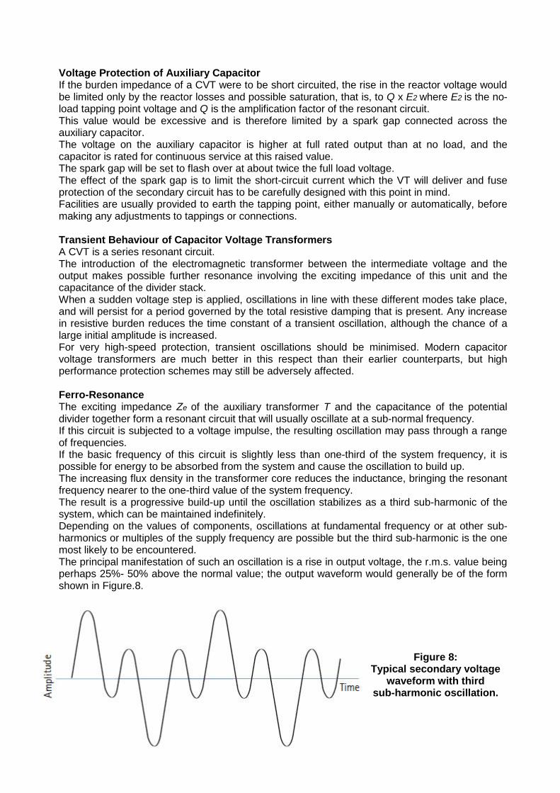
Voltage Protection of Auxiliary Capacitor If the burden impedance of a CVT were to be short circuited, the rise in the reactor voltage would be limited only by the reactor losses and possible saturation, that is, to Q x E2 where E2 is the no-load tapping point voltage and Q is the amplification factor of the resonant circuit. This value would be excessive and is therefore limited by a spark gap connected across the auxiliary capacitor. The voltage on the auxiliary capacitor is higher at full rated output than at no load, and the capacitor is rated for continuous service at this raised value. The spark gap will be set to flash over at about twice the full load voltage. The effect of the spark gap is to limit the short-circuit current which the VT will deliver and fuse protection of the secondary circuit has to be carefully designed with this point in mind. Facilities are usually provided to earth the tapping point, either manually or automatically, before making any adjustments to tappings or connections. Transient Behaviour of Capacitor Voltage Transformers A CVT is a series resonant circuit. The introduction of the electromagnetic transformer between the intermediate voltage and the output makes possible further resonance involving the exciting impedance of this unit and the capacitance of the divider stack. When a sudden voltage step is applied, oscillations in line with these different modes take place, and will persist for a period governed by the total resistive damping that is present. Any increase in resistive burden reduces the time constant of a transient oscillation, although the chance of a large initial amplitude is increased. For very high-speed protection, transient oscillations should be minimised. Modern capacitor voltage transformers are much better in this respect than their earlier counterparts, but high performance protection schemes may still be adversely affected. Ferro-Resonance The exciting impedance Ze of the auxiliary transformer T and the capacitance of the potential divider together form a resonant circuit that will usually oscillate at a sub-normal frequency. If this circuit is subjected to a voltage impulse, the resulting oscillation may pass through a range of frequencies. If the basic frequency of this circuit is slightly less than one-third of the system frequency, it is possible for energy to be absorbed from the system and cause the oscillation to build up. The increasing flux density in the transformer core reduces the inductance, bringing the resonant frequency nearer to the one-third value of the system frequency. The result is a progressive build-up until the oscillation stabilizes as a third sub-harmonic of the system, which can be maintained indefinitely. Depending on the values of components, oscillations at fundamental frequency or at other sub-harmonics or multiples of the supply frequency are possible but the third sub-harmonic is the one most likely to be encountered. The principal manifestation of such an oscillation is a rise in output voltage, the r.m.s. value being perhaps 25%- 50% above the normal value; the output waveform would generally be of the form shown in Figure.8.

Figure 8: Typical secondary voltage

waveform with third sub-harmonic oscillation.

44

Such oscillations are less likely to occur when the circuit losses are high, as is the case with a resistive burden, and can be prevented by increasing the resistive burden. Special anti-ferro-resonance devices that use a parallel tuned circuit are sometimes built into the VT. Although such arrangements help to suppress ferro-resonance, they tend to impair the transient response, so that the design is a matter of compromise. Correct design will prevent a CVT that supplies a resistive burden from exhibiting this effect, but it is possible for non-linear inductive burdens, such as auxiliary voltage transformers, to induce ferro-resonance. Auxiliary voltage transformers for use with capacitor voltage transformers should be designed with a low value of flux density that prevents transient voltages from causing core saturation, which in turn would bring high exciting currents.

Current transformers The primary winding of a current transformer is connected in series with the power circuit and the impedance is negligible compared with that of the power circuit. The power system impedance governs the current passing through the primary winding of the current transformer. This condition can be represented by inserting the load impedance, referred through the turns ratio, in the input connection of Figure 1. This approach is developed in Figure 9, taking the numerical example of a 300/5A CT applied to an 11kV power system. The system is considered to be carrying rated current (300A) and the CT is feeding a burden of 10VA. A study of the final equivalent circuit of Figure 9(c), taking note of the typical component values, will reveal all the properties of a current transformer. It will be seen that: a. the secondary current will not be affected by change of the burden impedance over a considerable range b. the secondary circuit must not be interrupted while the primary winding is energised. The induced secondary e.m.f. under these circumstances will be high enough to present a danger to life and insulation c. the ratio and phase angle errors can be calculated easily if the magnetising characteristics and the burden impedance are known

Figure 9: Derivation of equivalent

circuit of a current transformer

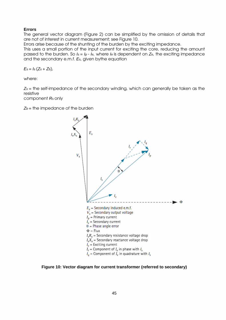
45

Errors The general vector diagram (Figure 2) can be simplified by the omission of details that are not of interest in current measurement; see Figure 10. Errors arise because of the shunting of the burden by the exciting impedance. This uses a small portion of the input current for exciting the core, reducing the amount passed to the burden. So Is = Ip - Ie, where Ie is dependent on Ze, the exciting impedance and the secondary e.m.f. Es, given bythe equation Es = Is (Zs + Zb), where: Zs = the self-impedance of the secondary winding, which can generally be taken as the resistive component Rs only Zb = the impedance of the burden

Figure 10: Vector diagram for current transformer (referred to secondary)

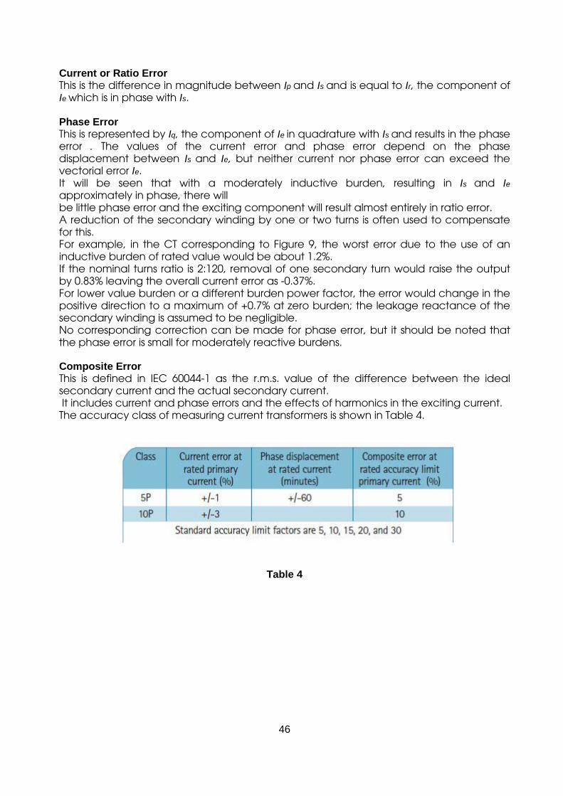
46

Current or Ratio Error This is the difference in magnitude between Ip and Is and is equal to Ir, the component of Ie which is in phase with Is. Phase Error This is represented by Iq, the component of Ie in quadrature with Is and results in the phase error . The values of the current error and phase error depend on the phase displacement between Is and Ie, but neither current nor phase error can exceed the vectorial error Ie. It will be seen that with a moderately inductive burden, resulting in Is and Ie approximately in phase, there will be little phase error and the exciting component will result almost entirely in ratio error. A reduction of the secondary winding by one or two turns is often used to compensate for this. For example, in the CT corresponding to Figure 9, the worst error due to the use of an inductive burden of rated value would be about 1.2%. If the nominal turns ratio is 2:120, removal of one secondary turn would raise the output by 0.83% leaving the overall current error as -0.37%. For lower value burden or a different burden power factor, the error would change in the positive direction to a maximum of +0.7% at zero burden; the leakage reactance of the secondary winding is assumed to be negligible. No corresponding correction can be made for phase error, but it should be noted that the phase error is small for moderately reactive burdens. Composite Error This is defined in IEC 60044-1 as the r.m.s. value of the difference between the ideal secondary current and the actual secondary current. It includes current and phase errors and the effects of harmonics in the exciting current. The accuracy class of measuring current transformers is shown in Table 4.

Table 4

47

Accuracy Limit Current Of Protection Current Transformers Protection equipment is intended to respond to fault conditions, and is for this reason required to function at current values above the normal rating. Protection class current transformers must retain a reasonable accuracy up to the largest relevant current. This value is known as the ‘accuracy limit current’ and may be expressed in primary or equivalent secondary terms. The ratio of the accuracy limit current to the rated current is known as the 'accuracy limit factor'. The accuracy class of protection current transformers is shown in Table 5.

Table 5.

48

Even though the burden of a protection CT is only a few VA at rated current, the output required from the CT may be considerable if the accuracy limit factor is high. For example, with an accuracy limit factor of 30 and a burden of 10VA, the CT may have to supply 9000VA to the secondary circuit. Alternatively, the same CT may be subjected to a high burden. For overcurrent and earth fault protection, with elements of similar VA consumption at setting, the earth fault element of an electromechanical relay set at 10% would have 100 times the impedance of the overcurrent elements set at 100%. Although saturation of the relay elements somewhat modifies this aspect of the matter, it will be seen that the earth fault element is a severe burden, and the CT is likely to have a considerable ratio error in this case. So it is not much use applying turns compensation to such current transformers; it is generally simpler to wind the CT with turns corresponding to the nominal ratio. Current transformers are often used for the dual duty of measurement and protection. They will then need to be rated according to a class selected from both Tables 4 and 5. The applied burden is the total of instrument and relay burdens. Turns compensation may well be needed to achieve the measurement performance. Measurement ratings are expressed in terms of rated burden and class, for example 15VA Class 0.5. Protection ratings are expressed in terms of rated burden, class, and accuracy limit factor, for example 10VA Class 10P10.

Figure.11: Definition of knee-point of excitation curve

49

Class PX Current Transformers The classification of Table 6.5 is only used for overcurrent protection. Class PX is the definition in IEC 60044-1 for the quasi-transient current transformers formerly covered by Class X of BS 3938, commonly used with unit protection schemes. Guidance was given in the specifications to the application of current transformers to earth fault protection, but for this and for the majority of other protection applications it is better to refer directly to the maximum useful e.m.f. that can be obtained from the CT. In this context, the 'knee-point' of the excitation curve is defined as 'that point at which a further increase of 10% of secondary e.m.f. would require an increment of exciting current of 50%’; see Figure 11. Design requirements for current transformers for general protection purposes are frequently laid out in terms of knee-point e.m.f., exciting current at the knee-point (or some other specified point) and secondary winding resistance. Such current transformers are designated Class PX. CT Winding Arrangements A number of CT winding arrangements are used. These are described in the following sections. Wound primary type This type of CT has conventional windings formed of copper wire wound round a core. It is used for auxiliary current transformers and for many low or moderate ratio current transformers used in switchgear of up to 11kV rating. Bushing or bar primary type Many current transformers have a ring-shaped core, sometimes built up from annular stampings, but often consisting of a single length of strip tightly wound to form a close-turned spiral. The distributed secondary winding forms a toroid which should occupy the whole perimeter of the core, a small gap being left between start and finish leads for insulation. Such current transformers normally have a single concentrically placed primary conductor, sometimes permanently built into the CT and provided with the necessary primary insulation. In other cases, the bushing of a circuit breaker or power transformer is used for this purpose. At low primary current ratings it may be difficult to obtain sufficient output at the desired accuracy. This is because a large core section is needed to provide enough flux to induce the secondary e.m.f. in the small number of turns, and because the exciting ampere-turns form a large proportion of the primary ampere-turns available. The effect is particularly pronounced when the core diameter has been made large so as to fit over large EHV bushings. Core-balance current transformers The core-balance CT (or CBCT) is normally of the ring type, through the centre of which is passed cable that forms the primary winding. An earth fault relay, connected to the secondary winding, is energised only when there is residual current in the primary system. The advantage in using this method of earth fault protection lies in the fact that only one CT core is used in place of three phase CT's whose secondary windings are residually connected. In this way the CT magnetising current at relay operation is reduced by approximately three-to-one, an important consideration in sensitive earth fault relays where a low effective setting is required. The number of secondary turns does not need to be related to the cable rated current because no secondary current would flow under normal balanced conditions. This allows the number of secondary turns to be chosen such as to optimise the effective primary pickup current.

50

Core-balance transformers are normally mounted over a cable at a point close up to the cable gland of switchgear or other apparatus. Physically split cores ('slip-over' types) are normally available for applications in which the cables are already made up, as on existing switchgear.

51

Summation current transformers The summation arrangement is a winding arrangement used in a measuring relay or on an auxiliary current transformer to give a single-phase output signal having a specific relationship to the three-phase current input. Air-gapped current transformers These are auxiliary current transformers in which a small air gap is included in the core to produce a secondary voltage output proportional in magnitude to current in the primary winding. Sometimes termed 'transactors' and 'quadrature current transformers', this form of current transformer has been used as an auxiliary component of unit protection schemes in which the outputs into multiple secondary circuits must remain linear for and proportioned to the widest practical range of input currents. Line Current CT’s CT’s for measuring line currents fall into one of three types. Overdimensioned CT’s Overdimensioned CT’s are capable of transforming fully offset fault currents without distortion. In consequence, they are very large, as can be deduced from Section 6.4.10. They are prone to errors due to remanent flux arising, for instance, from the interruption of heavy fault currents. Anti-remanence CT’s This is a variation of the overdimensioned current transformer and has small gap(s) in the core magnetic circuit, thus reducing the possible remanent flux from approximately 90% of saturation value to approximately 10%. These gap(s) are quite small, for example 0.12mm total, and so the excitation characteristic is not significantly changed by their presence. However, the resulting decrease in possible remanent core flux confines any subsequent d.c. flux excursion, resulting from primary current asymmetry, to within the core saturation limits. Errors in current transformation are therefore significantly reduced when compared with those with the gapless type of core. Transient protection current transformers are included in IEC 60044-6 as types TPX, TPY and TPZ and this specification gives good guidance to their application and use.

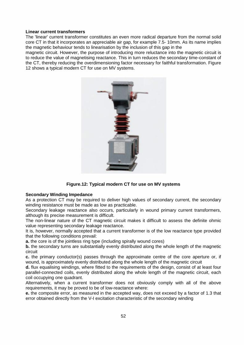
52

Linear current transformers The 'linear' current transformer constitutes an even more radical departure from the normal solid core CT in that it incorporates an appreciable air gap, for example 7.5- 10mm. As its name implies the magnetic behaviour tends to linearisation by the inclusion of this gap in the magnetic circuit. However, the purpose of introducing more reluctance into the magnetic circuit is to reduce the value of magnetising reactance. This in turn reduces the secondary time-constant of the CT, thereby reducing the overdimensioning factor necessary for faithful transformation. Figure 12 shows a typical modern CT for use on MV systems.

Figure.12: Typical modern CT for use on MV systems Secondary Winding Impedance As a protection CT may be required to deliver high values of secondary current, the secondary winding resistance must be made as low as practicable. Secondary leakage reactance also occurs, particularly in wound primary current transformers, although its precise measurement is difficult. The non-linear nature of the CT magnetic circuit makes it difficult to assess the definite ohmic value representing secondary leakage reactance. It is, however, normally accepted that a current transformer is of the low reactance type provided that the following conditions prevail: a. the core is of the jointless ring type (including spirally wound cores) b. the secondary turns are substantially evenly distributed along the whole length of the magnetic circuit c. the primary conductor(s) passes through the approximate centre of the core aperture or, if wound, is approximately evenly distributed along the whole length of the magnetic circuit d. flux equalising windings, where fitted to the requirements of the design, consist of at least four parallel-connected coils, evenly distributed along the whole length of the magnetic circuit, each coil occupying one quadrant. Alternatively, when a current transformer does not obviously comply with all of the above requirements, it may be proved to be of low-reactance where: e. the composite error, as measured in the accepted way, does not exceed by a factor of 1.3 that error obtained directly from the V-I excitation characteristic of the secondary winding

53

Secondary Current Rating The choice of secondary current rating is determined largely by the secondary winding burden and the standard practice of the user. Standard CT secondary current ratings are 5A and 1A. The burden at rated current imposed by digital or numerical relays or instruments is largely independent of the rated value of current. This is because the winding of the device has to develop a given number of ampere-turns at rated current, so that the actual number of turns is inversely proportional to the current, and the impedance of the winding varies inversely with the square of the current rating. However, electromechanical or static earth-fault relays may have a burden that varies with the current tapping used. Interconnection leads do not share this property, however, being commonly of standard cross-section regardless of rating. Where the leads are long, their resistance may be appreciable, and the resultant burden will vary with the square of the current rating. For example a CT lead run of the order of 200 metres, a typical distance for outdoor EHV switchgear, could have a loop resistance of approximately 3 ohms. The CT lead VA burden if a 5A CT is used would be 75VA, to which must be added the relay burden (up to of perhaps 10VA for an electromechanical relay, but less than 1VA for a numerical relay), making a total of 85VA. Such a burden would require the CT to be very large and expensive, particularly if a high accuracy limit factor were also applicable. With a 1A CT secondary rating, the lead burden is reduced to 3VA, so that with the same relay burden the total becomes a maximum of 13VA. This can be provided by a CT of normal dimensions, resulting in a saving in size, weight and cost. Hence modern CT’s tend to have secondary windings of 1A rating. However, where the primary rating is high, say above 2000A, a CT of higher secondary rating may be used, to limit the number of secondary turns. In such a situation secondary ratings of 2A, 5A or, in extreme cases, 20A, might be used. Rated Short-Time Current A current transformer is overloaded while system shortcircuit currents are flowing and will be short-time rated. Standard times for which the CT must be able to carry rated short-time current (STC) are 0.25, 0.5, 1.0, 2.0 or 3.0 seconds. A CT with a particular short-time current/ time rating will carry a lower current for a longer time in inverse proportion to the square of the ratio of current values. The converse, however, cannot be assumed, and larger current values than the S.T.C. rating are not permissible for any duration unless justified by a new rating test to prove the dynamic capability. Transient Response of a Current Transformer When accuracy of response during very short intervals is being studied, it is necessary to examine what happens when the primary current is suddenly changed. The effects are most important, and were first observed in connection with balanced forms of protection, which were liable to operate unnecessarily when short-circuit currents were suddenly established.

54

Primary current transient The power system, neglecting load circuits, is mostly inductive, so that when a short circuit occurs, the fault current that flows is given by: …

Equation 1

The first term of Equation 1 represents the steady state alternating current, while the second is a transient quantity responsible for displacing the waveform asymmetrically. is the steady state peak current Ip. The maximum transient occurs when no other condition need be examined. So:

Equation 2 When the current is passed through the primary winding of a current transformer, the response can be examined by replacing the CT with an equivalent circuit as shown in Figure 9(b). As the 'ideal' CT has no losses, it will transfer the entire function, and all further analysis can be carried out in terms of equivalent secondary quantities (is and Is). A simplified solution is obtainable by neglecting the exciting current of the CT. The flux developed in an inductance is obtained by integrating the applied e.m.f. through a time interval:

Equation .3

55

For the CT equivalent circuit, the voltage is the drop on the burden resistance Rb. Integrating for each component in turn, the steady state peak flux is given by:

Equation 4 The transient flux is given by:

Equation.5 Hence, the ratio of the transient flux to the steady state value is: where X and R are the primary system reactance and resistance values. The CT core has to carry both fluxes, so that:

Equation 6 The term (1+X/R) has been called the 'transient factor' (TF), the core flux being increased by this factor during the transient asymmetric current period. From this it can be seen that the ratio of reactance to resistance of the power system is an important feature in the study of the behaviour of protection relays. Alternatively, L/R is the primary system time constant T, so that the transient factor can be written: Again, fT is the time constant expressed in cycles of the a.c. quantity T’, so that:

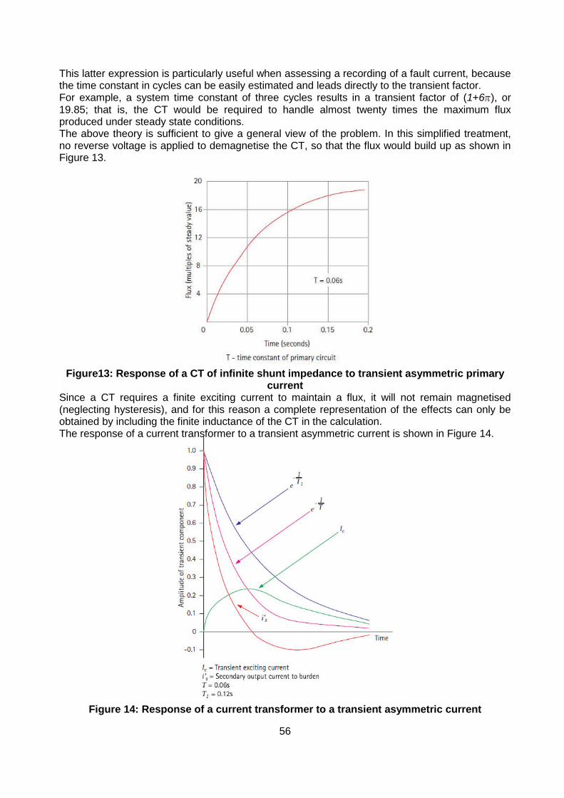
56

This latter expression is particularly useful when assessing a recording of a fault current, because the time constant in cycles can be easily estimated and leads directly to the transient factor. For example, a system time constant of three cycles results in a transient factor of (1+6 ), or 19.85; that is, the CT would be required to handle almost twenty times the maximum flux produced under steady state conditions. The above theory is sufficient to give a general view of the problem. In this simplified treatment, no reverse voltage is applied to demagnetise the CT, so that the flux would build up as shown in Figure 13.

Figure13: Response of a CT of infinite shunt impedance to transient asymmetric primary current

Since a CT requires a finite exciting current to maintain a flux, it will not remain magnetised (neglecting hysteresis), and for this reason a complete representation of the effects can only be obtained by including the finite inductance of the CT in the calculation. The response of a current transformer to a transient asymmetric current is shown in Figure 14.

Figure 14: Response of a current transformer to a transient asymmetric current

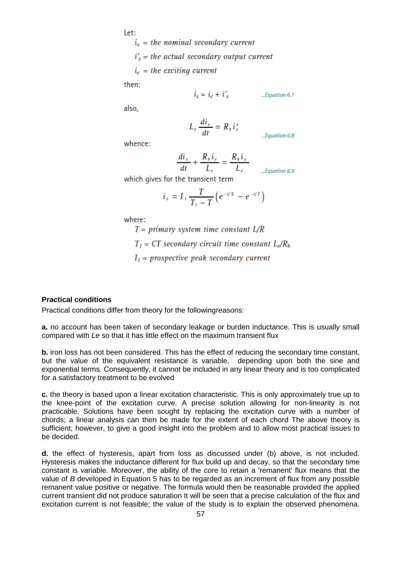
57

Practical conditions Practical conditions differ from theory for the followingreasons: a. no account has been taken of secondary leakage or burden inductance. This is usually small compared with Le so that it has little effect on the maximum transient flux b. iron loss has not been considered. This has the effect of reducing the secondary time constant, but the value of the equivalent resistance is variable, depending upon both the sine and exponential terms. Consequently, it cannot be included in any linear theory and is too complicated for a satisfactory treatment to be evolved c. the theory is based upon a linear excitation characteristic. This is only approximately true up to the knee-point of the excitation curve. A precise solution allowing for non-linearity is not practicable. Solutions have been sought by replacing the excitation curve with a number of chords; a linear analysis can then be made for the extent of each chord The above theory is sufficient, however, to give a good insight into the problem and to allow most practical issues to be decided. d. the effect of hysteresis, apart from loss as discussed under (b) above, is not included. Hysteresis makes the inductance different for flux build up and decay, so that the secondary time constant is variable. Moreover, the ability of the core to retain a 'remanent' flux means that the value of B developed in Equation 5 has to be regarded as an increment of flux from any possible remanent value positive or negative. The formula would then be reasonable provided the applied current transient did not produce saturation It will be seen that a precise calculation of the flux and excitation current is not feasible; the value of the study is to explain the observed phenomena.

58

The asymmetric (or d.c.) component can be regarded as building up the mean flux over a period corresponding to several cycles of the sinusoidal component, during which period the latter component produces a flux swing about the varying 'mean level' established by the former. The asymmetric flux ceases to increase when the exciting current is equal to the total asymmetric input current, since beyond this point the output current, and hence the voltage drop across the burden resistance, is negative. Saturation makes the point of equality between the excitation current and the input occur at a flux level lower than would be expected from linear theory. When the exponential component drives the CT into saturation, the magnetising inductance decreases, causing a large increase in the alternating component ie. The total exciting current during the transient period is of the form shown in Figure 15 and the corresponding resultant distortion in the secondary current output, due to saturation, is shown in Figure 16.

Figure 15: Typical exciting current of CT during transient asymmetric input current

Figure 16: Distortion in secondary current due to saturation

59

The presence of residual flux varies the starting point of the transient flux excursion on the excitation characteristic. Remanence of like polarity to the transient will reduce the value of symmetric current of given time constant which the CT can transform without severe saturation; conversely, reverse remanence will greatly increase the ability of a CT to transform transient current. If the CT were the linear non-saturable device considered in the analysis, the sine current would be transformed without loss of accuracy. In practice the variation in excitation inductance caused by transferring the centre of the flux swing to other points on the excitation curve causes an error that may be very large. The effect on measurement is of little consequence, but for protection equipment that is required to function during fault conditions, the effect is more serious. The output current is reduced during transient saturation, which may prevent the relays from operating if the conditions are near to the relay setting. This must not be confused with the increased r.m.s. value of the primary current due to the asymmetric transient, a feature which sometimes offsets the increase ratio error. In the case of balanced protection, during through faults the errors of the several current transformers may differ and produce an out-ofbalance quantity, causing unwanted operation. Harmonics during the Transient Period When a CT is required to develop a high secondary e.m.f. under steady state conditions, the non-linearity of the excitation impedance causes some distortion of the output waveform; such a waveform will contain, in addition to the fundamental current, odd harmonics only. When, however, the CT is saturated uni-directionally while being simultaneously subjected to a small a.c. quantity, as in the transient condition discussed above, the output will contain both odd and even harmonics. Usually the lower numbered harmonics are of greatest amplitude and the second and third harmonic components may be of considerable value. This may affect relays that are sensitive to harmonics. Test Windings On-site conjunctive testing of current transformers and the apparatus that they energise is often required. It may be difficult, however, to pass a suitable value of current through the primary windings, because of the scale of such current and in many cases because access to the primary conductors is difficult. Additional windings may be provided to make such tests easier, these windings usually being rated at 10A. The test winding will inevitably occupy appreciable space and the CT will cost more. This fact should be weighed against the convenience achieved; very often it will be found that the tests in question can be replaced by alternative procedures.

Novel instrument transformers The preceding types of instrument transformers have all been based on electromagnetic principles using a magnetic core. There are now available several new methods of transforming the measured quantity using optical and mass state methods.

60

Optical Instrument Transducers The key features of a freestanding optical instrument transducer can be illustrated with the functional diagram of Figure 17.

Figure 17: Functional diagram of optical instrument transducer Optical converters and optical glass fibre channels implement the link between the sensor and the low voltage output. The fundamental difference between an instrument transducer and a conventional instrument transformer is the electronic interface needed for its operation. This interface is required both for the sensing function and for adapting the new sensor technology to that of the secondary output currents and voltages. Non-conventional optical transducers lend themselves to smaller, lighter devices where the overall size and power rating of the unit does not have any significant bearing on the size and the complexity of the sensor. Small, lightweight insulator structures may be tailor-made to fit optical sensing devices as an integral part of the insulator. Additionally, the non-linear effects and electromagnetic interference problems in the secondary wiring of conventional VT’s and CT’s are minimised. Optical transducers can be separated in two families: firstly the hybrid transducers, making use of conventional electrical circuit techniques to which are coupled various optical converter systems, and secondly the ‘all-optical’ transducers that are based on fundamental, optical sensing principles.

61

Optical sensor concepts Certain optical sensing media (glass, crystals, plastics) show a sensitivity to electric and magnetic fields and that some properties of a probing light beam can be altered when passing through them. One simple optical transducer description is given here in Figure. 18. Consider the case of a beam of light passing through a pair of polarising filters. If the input and output polarising filters have their axes rotated 45° from each other, only half the light will come through. The reference light input intensity is maintained constant over time. Now if these two polarising filters remain fixed and a third polarising filter is placed in between them, a random rotation of this middle polariser either clockwise or counter-clockwise will be monitored as a varying or modulated light output intensity at the light detector. When a block of optical sensing material (glass or crystal) is immersed in a varying magnetic or electric field, it plays the role of the ‘odd’ polariser. Changes in the magnetic or electric field in which the optical sensor is immersed are monitored as a varying intensity of the probing light beam at the light detector. The light output intensity fluctuates around the zero-field level equal to 50% of the reference light input. This modulation of the light intensity due to the presence of varying fields is converted back to time-varying currents or voltages. A transducer uses a magneto-optic effect sensor for optical current measuring applications. This reflects the fact that the sensor is not basically sensitive to a current but to the magnetic field generated by this current. Although ‘all-fibre’ approaches are feasible, most commercially available optical current transducers rely on a bulk-glass sensor. Most optical voltage transducers, on the other hand, rely on an electro-optic effect sensor. This reflects the fact that the sensor used is sensitive to the imposed electric field.

62

Hybrid transducers The hybrid family of non-conventional instrument transducers can be divided in two types: those with active sensors and those with passive sensors. The idea behind a transducer with an active sensor is to change the existing output of the conventional instrument transformer into an optically isolated output by adding an optical conversion system (Figure 18). Figure. 18: Schematic representation of the concepts behind the optical sensing of varying

electric and magnetic fields This conversion system may require a power supply of its own: this is the active sensor type. The use of an optical isolating system serves to de-couple the instrument transformer output secondary voltages and currents from earthed or galvanic links. Thus the only link that remains between the control-room and the switchyard is a fibre optic cable. Another type of hybrid non-conventional instrument transformer is achieved by retrofitting a passive optical sensing medium into a conventional ‘hard-wire secondary’ instrument transformer. This can be termed as a passive hybrid type since no power supply of any kind is needed at the secondary level.

‘All-optical’ transducers These instrument transformers are based entirely on optical materials and are fully passive. The sensing function is achieved directly by the sensing material and a simple fibre optic cable running between the base of the unit and the sensor location provides the communication link. The sensing element is made of an optical material that is positioned in the electric or magnetic field to be sensed. In the case of a current measuring device the sensitive element is either located free in the magnetic field (Figure 19(a)) or it can be immersed in a field-shaping magnetic ‘gap’ (Figure 19(b)). In the case of a voltage-sensing device (Figure 20) the same alternatives exist, this time for elements that are sensitive to electric fields.

63

The possibility exists of combining both sensors within a single housing, thus providing both a CT and VT within a single compact housing that gives rise to space savings within a substation.

Figure 19: Optical current sensor based on the magnetic properties of optical materials

In all cases there is an optical fibre that channels the probing reference light from a source into the medium and another fibre that channels the light back to analysing circuitry. In sharp contrast with a conventional free-standing instrument transformer, the optical instrument transformer needs an electronic interface module in order to function. Therefore its sensing principle (the optical material) is passive but its operational integrity relies on the interface that is powered in the control room (Figure 21).

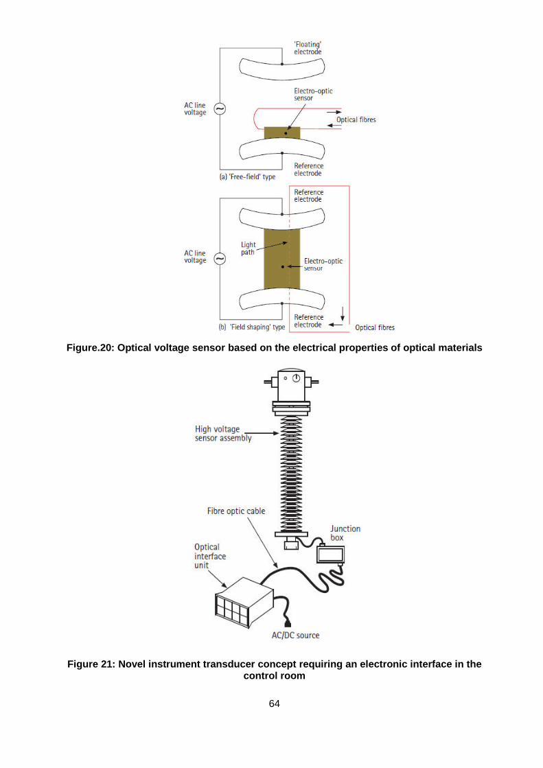
64

Figure.20: Optical voltage sensor based on the electrical properties of optical materials

Figure 21: Novel instrument transducer concept requiring an electronic interface in the control room

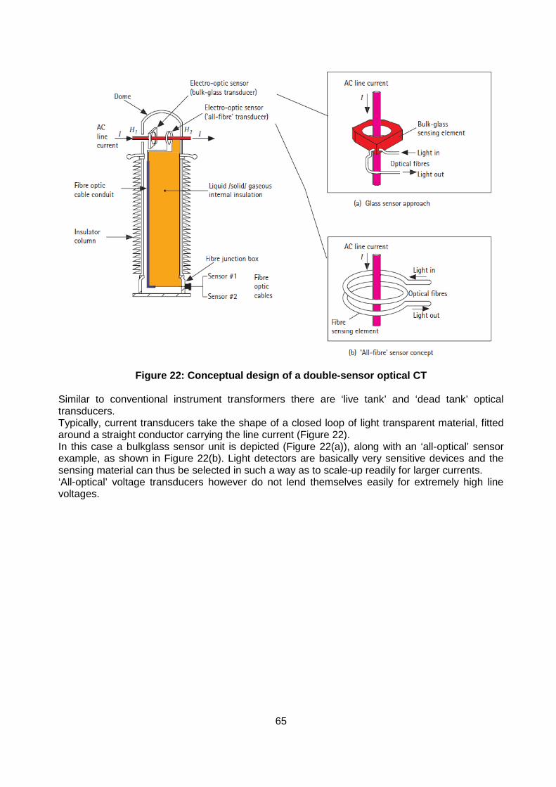
65

Figure 22: Conceptual design of a double-sensor optical CT Similar to conventional instrument transformers there are ‘live tank’ and ‘dead tank’ optical transducers. Typically, current transducers take the shape of a closed loop of light transparent material, fitted around a straight conductor carrying the line current (Figure 22). In this case a bulkglass sensor unit is depicted (Figure 22(a)), along with an ‘all-optical’ sensor example, as shown in Figure 22(b). Light detectors are basically very sensitive devices and the sensing material can thus be selected in such a way as to scale-up readily for larger currents. ‘All-optical’ voltage transducers however do not lend themselves easily for extremely high line voltages.

66

Figure 23: Optical voltage transducer concepts, using a ‘full-voltage’ sensor Although ‘all-optical’ instrument transformers were first introduced 10-15 years ago, there are still only a few in service nowadays. Figure 24 shows a field installation of a combined optical CT/VT.

Figure 24: Field installation of a combined optical CT/VT

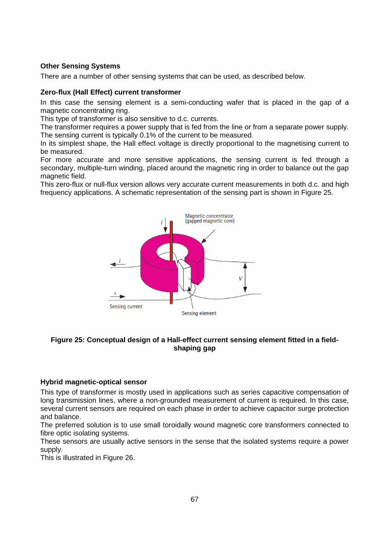
67

Other Sensing Systems There are a number of other sensing systems that can be used, as described below.

Zero-flux (Hall Effect) current transformer In this case the sensing element is a semi-conducting wafer that is placed in the gap of a magnetic concentrating ring. This type of transformer is also sensitive to d.c. currents. The transformer requires a power supply that is fed from the line or from a separate power supply. The sensing current is typically 0.1% of the current to be measured. In its simplest shape, the Hall effect voltage is directly proportional to the magnetising current to be measured. For more accurate and more sensitive applications, the sensing current is fed through a secondary, multiple-turn winding, placed around the magnetic ring in order to balance out the gap magnetic field. This zero-flux or null-flux version allows very accurate current measurements in both d.c. and high frequency applications. A schematic representation of the sensing part is shown in Figure 25.

Figure 25: Conceptual design of a Hall-effect current sensing element fitted in a field-shaping gap

Hybrid magnetic-optical sensor This type of transformer is mostly used in applications such as series capacitive compensation of long transmission lines, where a non-grounded measurement of current is required. In this case, several current sensors are required on each phase in order to achieve capacitor surge protection and balance. The preferred solution is to use small toroidally wound magnetic core transformers connected to fibre optic isolating systems. These sensors are usually active sensors in the sense that the isolated systems require a power supply. This is illustrated in Figure 26.

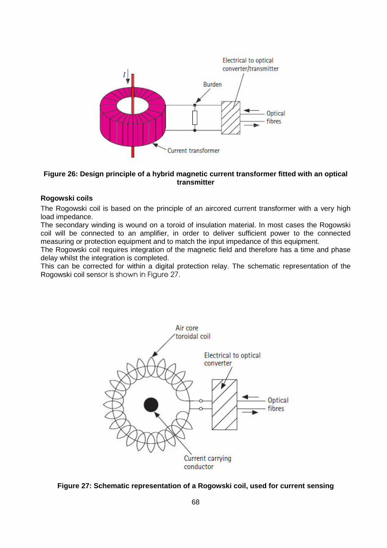
68

Figure 26: Design principle of a hybrid magnetic current transformer fitted with an optical transmitter

Rogowski coils The Rogowski coil is based on the principle of an aircored current transformer with a very high load impedance. The secondary winding is wound on a toroid of insulation material. In most cases the Rogowski coil will be connected to an amplifier, in order to deliver sufficient power to the connected measuring or protection equipment and to match the input impedance of this equipment. The Rogowski coil requires integration of the magnetic field and therefore has a time and phase delay whilst the integration is completed. This can be corrected for within a digital protection relay. The schematic representation of the Rogowski coil sensor is shown in Figure 27.

Figure 27: Schematic representation of a Rogowski coil, used for current sensing

69