Test Generation for Duration SystemsSaddek Bensalem, Lotfi Majdoub, Stavros Tripakis

Moez Krichen Riadh Robbana Verimag Laboratory andVerimag Laboratory, LIP2 Laboratory and Cadence Berkeley Labs,Centre Equation 2, Polytechnic School of Tunisia 1995 University avenue,avenue de Vignate, lotfi.majdoub@ensi.rnu.tn, Suite 460, Berkeley,

38610, Gieres, France. riadh.robbana@fst.rnu.tn CA 94704, USA.saddek.bensalem@imag.fr, tripakis@cadence.com

moez.krichen@imag.fr

Abstract

We are interested in generating tests for duration systems modeling real-timesystems. The specification of a duration system is given as a duration graph.Duration graphs are an extension of timed graphs and are suitable for modeling theaccumulated times spent by computations within the considered duration system.In this paper, we present a method for generating tests for duration systems basedon the so-called approximation method. First, we use the approximation method toextend the specification model into an approximate model. The latter contains thedigitization computations of the initial model. Test trees are then extracted from theapproximate model. We explain how the obtained digital-test trees can be executed inan analog-fashion.

Keywords: Real-Time, Duration Systems, Testing, Approximation method, Digitization.

1. INTRODUCTION

Duration systems are real-time systems. A duration system encodes both constraints on thedelays separating consecutive discrete events as well as constraints on accumulated delays spentby a given computation of the system.

Timed graphs (also called timed automata) constitute a powerful formalism widely adopted formodeling real-time systems [2]. Duration Variable Timed Graphs (DVTG for short) [4] arean extension of the timed graph model. They are used as a formalism to describe durationsystems. A given DVTG has a finite set of continuous real variables that can be stopped insome locations (rate=0) and resumed in some other locations (rate=1). These variables are calledduration variables. They can model some temporal behaviors of a real-time system such as theaccumulated delays spent by some computations at some particular locations.

Testing is an important validation activity with a wide range of goals. In this work, we are interestedin conformance testing. Conformance testing aims to check whether a given implementationconforms to its specification. The testing procedure consists in generating test cases by derivingthem from the specification and then applying them to the implementation under test (IUT). Forthe case of real-time systems, conformance is defined with respect to both discrete actionsoccurrence and time elapsing. That is, for the IUT to be conforming to the specification it mustgenerate correct outputs at correct timings.

VECoS’2007 1

Generating exhaustive test remains expensive and in some cases impossible, in particular forreal-time systems. Springintveld et al [16] proved that exhaustive testing of deterministic timedautomata with dense time is theoretically possible, but highly infeasible. Hence, some worksdefine a criteria for selecting test cases that is generated automatically such as coverage criteria(e.g., transition and location coverage) [8, 9, 11]. Other works try to define purposes of test andgenerating test cases according to those purposes [14, 12]. An other way to alleviate this problemis the following.

For testing real-time systems, most works [3, 6, 9, 10, 11, 13] use discretization techniquesto reduce the infinite state space into a finite (or at least countable) state space then adaptthe existing untimed test case generation algorithm [17]. There is a lot of similarities between(model-based) testing and system verification. People working on real-time testing borrow alot of techniques from the real-time verification field to generate test cases automatically (e.g.,discretization techniques based on the so-called region graph, model checking techniques, etc.).[8] show how it is possible to represent coverage criteria and test purposes as a reachabilityproperty and use the model checking tool UPPAAL [8] to generate test cases with respect to theconsidered criteria.

It is well known that the verification of real time system is mainly possible thanks to the decidabilityof the reachability problem for systems represented as timed automata [1]. On the other side, ithas been shown that the reachability problem is undecidable for timed graphs extended with oneduration variable [5]. Consequently it is less obvious to use the classical verification techniquesfor testing DVTG.

In this paper, we propose a test generation method for duration systems. We use theapproximation method extending a given DVTG-IO specification to another specification calledapproximate model. Our method consists of generating tests from the approximate model. Thebehavior of a test is derived from the approximate specification model. It is described by a tree,called test tree. In order to construct the test tree, we adapt the untimed test generation algorithmof [17] and apply it to the approximate specification model. We also give the way of how theobtained test trees shall be executed.

The rest of the paper is organized as follows. Section 2 introduces the DVTG model. Section 4gives the approximation method. Section 5 defines the type of tests we consider. Section 6 givesour testing method and shows how test trees are derived from the approximate model. Concludingremarks are presented in section 7.

2. DURATION VARIABLE TIMED GRAPHS WITH INPUTS AND OUTPUTS (DVTG-IO)

In this section, we introduce the formalism we use for describing duration systems, called durationvariable timed graph with inputs and outputs (DVTG-IO for short).1 DVTG-IO is an extension ofthe well-known timed automata model defined in [2]. We give here the formal definition and theoperational semantics of this model. Then, we present some terminologies that will be used in ourtest method. In the last subsection, we illustrate with a simple example.

2.1. The DVTG-IO model

A DVTG-IO is described by a finite set of locations and a transition relation between theselocations. In addition, the system has a finite set of duration variables that are constant slopecontinuous variables, each of them changes continuously with a rate in {0, 1} at each locationof the system. Transitions between locations are conditioned by arithmetical constraints on thevalues of the duration variables. When a transition is taken, a subset of duration variables shouldbe reset and an action should be executed, this action can be either an input action, an outputaction or an unobservable action.1A similar model to the DVTG-IO model is introduced in [4].

Test Generation for Duration Systems

We consider X a finite set of duration variables. A guard on X is a boolean combination ofconstraints of the form x ≺ c where x ∈ X and c ∈ N,≺∈ {<,≤, >,≥}. Let Γ(X) be the set ofguards on X.

A DVTG-IO is a tuple M = (Q, q0, E,X,Act, γ, α, δ, ∂) where:

• Q is a finite set of locations;• q0 is the initial location;• E ⊆ Q×Q is a finite set of transitions between locations;• Act = In ∪Out ∪ {τ} is the union of a finite set of input actions (a?, b?, c?, etc.), a finite set

of output actions (a!, b!, c!, etc.) and τ the unobservable action τ ;• γ : E −→ Γ(X) associates to each transition a guard which should be satisfied by the

duration variables whenever the transition is taken;• α : E −→ 2X gives for each transition the set of duration variables that should be reset when

the transition is taken;• δ : E −→ Act gives for each transition the action that should be executed when the transition

is taken;• ∂ : Q ×X −→ {0, 1} associates with each location q and each duration variable x the rate

at which x changes continuously while the computation is at q.

2.2. The state graph of a DVTG-IO

Let R+ be the set of nonnegative reals and N the set of nonnegative integers. The semantics ofa DVTG-IO are defined in terms of a state graph over states of the form s = (q, ν) where q ∈ Qand ν : X −→ R+. ν is a valuation function that assigns a real value to each duration variable.

Let SM be the set of states of M . Most of the time, SM is likely to contain infinitely many statessince the values of the duration variables are taken in R+. The initial state of a given DVTG-IO is(q0,

→0 ), where q0 is the initial location and

→0 the valuation assigning 0 to each duration variable.

Given a valuation ν and a guard g, we denote by ν |= g the fact that valuation of g under thevaluation ν is true.

We define two types of transitions between states.

1. Discrete Transitions of the form (q, ν) a (q′, ν′) where:

• (q, q′) ∈ E; δ(q, q′) = a;• ν |= γ(q, q′);• ∀x ∈ X \ α(q, q′) : ν′(x) = ν(x);• ∀x ∈ α(q, q′) : ν′(x) = 0.

2. Timed transitions of the form (q, ν) t (q, ν′) such that:

• t ∈ R;• ∀x ∈ X : ν′(x) = ν(x) + ∂(q, x) ∗ t.

The first type of transitions correspond to moves between locations due to the execution ofdiscrete actions from E. The second type of transitions correspond to time progress at somelocation q.

A path of the DVTG-IO is a sequence of transitions of the form

s0a1 s1

a2 s2 · · ·an−1 sn−1

an sn

such that:

• s0 = (q0,→0 );

• ∀i = 1, · · · , n : ai ∈ Act ∪R+;• ∀i = 1, · · · , n : si−1

ai si is a transition of the DVTG-IO.

Test Generation for Duration Systems

A state (q, ν) is called an integer state of SM if ν : X −→ N . We denote by N(SM ) the set ofinteger states of SM .

2.3. Computation sequences and timed words

We introduce the notion of computation sequences of a DVTG-IO. These sequences are definedas finite sequences of configurations. A configuration is a pair 〈s, t〉 where s is a state and t is atime value in R+. Let CM be the set of configurations of M .

A configuration 〈s, t〉 is called an integer configuration if t ∈ N . We denote by N(CM ) the set ofinteger configurations.

Clearly, we can easily make the link between states and configurations. A configuration can beseen as the state of the DVTG-IO extended with a new duration variable. The new duration variablemeasures the amount of time which has elapsed since the beginning of the computation. Thisduration variable is never stopped or reset. We call it the observation clock of the DVTG-IO. Forinstance, consider the path λ = s0

a1 s1a2 s2 · · ·

an−1 sn−1

an sn. The corresponding computationsequence is σ = 〈s0, t0〉

a1 〈s1, t1〉a2 〈s2, t2〉 · · ·

an−1 〈sn−1, tn−1〉

an 〈sn, tn〉 such that t0 = 0 and

∀i = 1, · · · , n : ti =i∑

k=1

time(ak) where time(ak) = 0 if ak ∈ Act; and time(ak) = ak if ak ∈ R+.

Each pair 〈si, ti〉 is called an extended state. We call CS(M) be the set of computation sequencesof M .

We introduce now the notion of timed words. A timed word is a finite sequence of timed actions.A timed action is a pair Jb, tK, where b ∈ Act and t ∈ R+. The pair Jb, tK means that action atook place precisely at time when the observation clock was equal to t. Thus a timed word is ofthe form ω = Jb1, t1KJb2, t2K · · · Jbn, tnK where for i = 1, · · · , n, bi ∈ Act and ti ∈ R+. If for eachi = 1, · · · , n, ti ∈ N then ω is said to be an integer timed word. Consider the following computationsequence σ = 〈s0, t0〉

a1 〈s1, t1〉a2 〈s2, t2〉 · · ·

an−1 〈sn−1, tn−1〉

an 〈sn, tn〉2 of the DVTG-IO M(i.e., σ ∈ CS(M)). Clearly, there exists a unique timed word ω corresponding to the computationsequence σ. The timed word ω is obtained as follows. Let 1 ≤ i1 < · · · < iN ≤ n such thatfor each j = 1, · · · , N , aij ∈ Act and for each i /∈ {i1, i2, · · · , iN}, ai ∈ R+. Then, the timedword corresponding to σ is ω = Jb1, t′1KJb2, t′2K · · · JbN , t′N K where for each j = 1, · · · , N : bj = aij ;

t′i =i∑

k=1

time(ak).

For simplicity, we may write: s0ω sn. The timed word ω is said to be an accepted timed word

of the DVTG-IO M . Let L(M) be the set of accepted timed words of M . We suppose that L(M)contains the empty timed word as well.

We need to introduce the notion of extended timed words as well. For the computation sequenceσ above, if an ∈ R+ then the corresponding extended timed word will be

ω� = Jb1, t′1KJb2, t′2K · · · JbN , t′N KJ � , t′N+1K

where

t′N+1 = tn =i∑

k=1

time(ak)

and � is a special symbol meaning that no discrete action took place within the interval (t′N , t′N+1].

We write s0ω� sn as well and ω� is said to be an accepted extended timed word of the DVTG-IO

M . We denote L�(M) the set of accepted timed words and extended timed words of M .

2We make the natural assumption that for each i = 1, · · · , n {ai−1, ai} 6⊆ R+. That is at least one of each two consecutivelabels is a discrete action from Act.

Test Generation for Duration Systems

We define the concatenation operator over timed words. For the two timed words ω1 and ω2 suchthat:

ω1 = Jb1, t′1KJb2, t′2K · · · Jbn, t′nK

andω2 = Jbn+1, t

′n+1KJbn+2, t

′n+2K · · · Jbn+m, t

′n+mK

we haveω1 · ω2 = Jb1, t′1KJb2, t

′2K · · · Jbn, t′nKJbn+1, t

′n+1K · · · Jbn+m, t

′n+mK.

By convention, for any tn, tn+1 ∈ Act and bn+1 ∈ Act we assume that:

J�, tnK · Jbn+1, tn+1K = Jbn+1, tn+1K.

2.4. An example of a DVTG-IO

A simple example od a DVTG-IO M is given in Figure 1 . The DVTG-IO has: 5 locations:{q0, q1, q2, q3, q4}; 2 input actions: {a?, c?}; 2 output actions: {b!, d!}; 3 durations variables {t, x, z}.

The initial location of the DVTG-IO is q0. The duration variable t is the observation clock of M . Itmeasures time elapsing since the beginning of each computation.

According to the figure, action a? is allowed to happen no later than one time-unit after thebeginning of the whole computation. Similarly, actions c? and d! shall happen exactly at t = 1and t = 2, respectively.

The guard “x = 1”, on the transition between locations q2 and q3, encodes the fact that the inputaction c? shall be emitted exactly one time-unit after the execution of a? (x is reset as soon as a?is emitted).

The duration variable z is stopped at both locations q1 and q3. Thus, it allows to measure the totalaccumulated time spent within the other locations (i.e., q0, q2 and q4).

3. THE CONFORMANCE RELATION TIOCO FOR DVTG-IO

3.1. Definition of tioco

In the sequel, for simplicity we consider only DVTG-IO all the actions of which are observable (i.e.,No transitions are labeled with τ ).

Next, we recall the definition of the timed input-output conformance relation tioco first introducedin [11] and which is in turn inspired from the “untimed” conformance relation ioco of [17].

The conformance relation tioco was initially introduced to the case of Timed automata with inputsand outputs. Next, we extend this relation in a straightforward way to the case of DVTG-IO. In orderto formally define the conformance relation, we define a number of operators. Given a DVTG-IOM and a timed word ω ∈ L�(M), M after ω is the set of all states of M that can be reached afterthe execution of the timed word ω.

Formally: M after ω = {s ∈ S(M) | : s0ω s} where s0 is the initial state of M . Given state

s ∈ S(M), elapse(s) is the set of all delays which can elapse from s without M making anyobservable action. Formally: elapse(s) = {t > 0 | ∃ s′ ∈ S(M) : s t

s′}.

Given state s ∈ S(M), out(s) is the set of all observable “events” (outputs or the passage of time)that can occur when the system is at state s. Formally:

out(s) = {a ∈ Out | ∃s′ ∈ S(M) : s a s′} ∪ elapse(s).

The definition naturally extends to a set of states S: out(S) =⋃s∈S

out(s).

Test Generation for Duration Systems

q0

q1z = 0

q3z = 0

q2

q4

b!

c?

d!t = 2 ∧ z = 1

x = 1

t = 1

x := 0

0 ≤ t ≤ 1 a?

FIGURE 1: An example of a DVTG-IO.

The timed input-output conformance relation, denoted tioco, is defined as

MI tioco MS ≡ ∀ω ∈ L�(MS) : out(MI after ω) ⊆ out(MS after ω).

The relation states that an implementation MI conforms to a specification MS if and only if for anyobservable behavior ω of MS , the set of observable outputs of MI after any behavior “matching”ω must be a subset of the set of possible observable outputs of MS .

Notice that observable outputs are not only observable output actions but also time delays.

3.2. Example

We consider the DVTG-IO M of Figure 1. We consider this DVTG-IO as the specification model.Three possible implementations of M are given in Figure 2, namely M1

I , M2I and M3

I . Amongthese three implementations only M3

I conforms to M with respect to tioco.

First, M1I ���tioco M since it produces a wrong output after receiving input a?. That is instead of

emitting output b! (as stated in the specification) it emits output d!. The (extended) timed word thatwe may use for detecting non-conformance is

ω� = Ja?, 0KJ�, 1K.

In fact we haveout(M after ω�) = {b!};

and

out(M1I after ω�) = {d!}.

First, M2I ���tioco M since it does not wait enough time before emitting output b! when it reaches

location q1 as stated in M . The timed word we may use in this case is simply

ω = Ja?, 0K.

Test Generation for Duration Systems

q0

q1z = 0

q2

b!t = 1

x := 0

0 ≤ t ≤ 1 a?

q0

q1z = 0

q3z = 0

q2

q4

b!

c?

d!t = 2 ∧ z = 1

x = 1

t = 0

x := 0

0 ≤ t ≤ 1 a?

q0

q1z = 0

q3z = 0

q2

q4

d!

c?

t = 2 ∧ z = 1

x = 1

t = 1

x := 0

0 ≤ t ≤ 1 a?

b!

M3IM1

I M2I

FIGURE 2: Possible implementations of the DVTG-IO given in Figure 1.

It is not difficult to see thatb! /∈ out(M after ω);

while

b! ∈ out(M1I after ω).

Finally, we clearly have M3I tioco M since the set of computation sequences of M3

I is a subset ofthe set of computation sequences of M . That is

CS(M3I ) ⊆ CS(M).

4. THE APPROXIMATION METHOD

The approximation method we introduce in this section bears some similarity with the methodproposed in [15]. This method is used for the verification of reachability properties for durationsystems.

Next, we describe the method and we show how we use it for testing real-time systems modeled asDVTG-IO. The approximation method we present is mainly based on the so-called discretizationtechnique. In [7], the latter is called digitization technique instead. It consists in associating adiscrete computation to each possible analog computation of the specification. We show withan example that the obtained discrete computations may not belong to the specification model.Thus, we propose an approximate model that contains all discrete computations. The approximatemodel is generated from the specification by the approximation method.

4.1. The digitization technique

We present the notion of digitization introduced in [7]. We adapt it to the case of the DVTG-IOmodel. We first introduce some definitions and notations. Let t ∈ R+ and n ∈ N . If t ∈ [n, n + 1)

Test Generation for Duration Systems

then we use the following notation: btc = n ; and dte = n+ 1. For instance we have: b819.3c = 819and d819.3e = 820.

For t ∈ R+ and ξ ∈ [0, 1), if t ≤ btc+ ξ then [t]ξ = btc. Otherwise, [t]ξ = dte.

For instance for t = 819.3:

• For ξ = 0.2, [819.3]0.2 = 820;• For ξ = 0.3, [819.3]0.3 = 819;• For ξ = 0.4, [819.3]0.4 = 819.

The real value ξ is called the digitization quantum. Clearly for ξ = 0, we have for any t ∈ R+:[t]0 = dte. Thus for any t ∈ R+ and ξ ∈ [0, 1), we have: t ∈ ( [t]ξ + ξ − 1 , [t]ξ + ξ ] which isequivalent to: −1 + ξ < t− [t]ξ ≤ ξ.

Next we extend the notion of digitization above to the case of computation sequences. For thatpurpose, consider the following computation sequence

σ = 〈(q0, ν0), t0〉a1 〈(q1, ν1), t1〉 · · ·

an 〈(qn, νn), tn〉.

It is not difficult to see that for each duration variable x of the DVTG-IO and each k = 1, · · · , n, wehave:

νk(x) =k−1∑

i=jk+1

∂(qi, x) ∗ (ti+1 − ti)

such thatjk = max( {−1 } ∪ { j | j ≤ k ∧ x ∈ α(qj , qj+1)} ).3

Given a digitization quantum ξ ∈ [0, 1), the digitization of the computation sequence σ is theinteger computation sequence

[σ]ξ = 〈(q0, νξ0), [t0]ξ〉aξ1 〈(q1, νξ1), [t1]ξ〉 · · ·

aξn 〈(qn, νξn), [tn]ξ〉.

where for each k = 1, · · · , n and for each duration variable x we have: νξk(x) = [νk(x)]ξ. We denote[(qk, νk)]ξ = (qk, ν

ξk).

The labels aξk are defined as follows. If ak ∈ Act then aξk = ak. Otherwise, aξk = [tk]ξ − [tk−1]ξ.

We denote Digit(CS(M)) the set of digitizations of all the real computation sequences of theDVTG-IO M . Notice that Digit(CS(M)) is a countable set while CS(M) is not.

We next extend the digitization technique to the case of timed words. Consider the following timedword

ω = Jb1, t1KJb2, t2K · · · Jbn, tnK.

For the digitization quantum ξ ∈ [0, 1), the integer timed word corresponding to ω is

[w]ξ = Jb1, [t1]ξKJb2, [t2]ξK · · · Jbn, [tn]ξK.

We denote Digit(L(M)) the set of digitizations of all the timed words accepted by the DVTG-IOM . Clearly, Digit(L(M)) is a countable set.

It is possible to make the general observation that the digitization technique allows to transforman uncountable set X to a countable one Digit(X).3The integer value jk corresponds to the last position at which x was reset before reaching the kth position.

Test Generation for Duration Systems

A legitimate question one may ask is whether Digit(X) ⊆ X or not. In our case given a DVTG-IOM , the question is

“Digit(CS(M)) ⊆ CS(M) or not?”.

Next we prove, by means of an example, that the statement above is not always true.

A counter example: We consider the DVTG-IO M given in Figure 1 . We give a computationsequence of this DVTG-IO such that for any digitization quantum the corresponding integercomputation sequence is not a element of CS(M).

The computation sequence we consider is the following:

Count-Exmp

=

〈(q0, 0 , 0 , 0 ), 0 〉|

0.5↓

〈(q0, 0.5, 0.5, 0.5), 0.5〉|

a?↓

〈(q1, 0.5, 0 , 0.5), 0.5〉|

0.5↓

〈(q1, 1 , 0.5, 0.5), 1 〉|b!↓

〈(q2, 1 , 0.5, 0.5), 1 〉|

0.5↓

〈(q2, 1.5, 1 , 1 ), 1.5〉|

c?↓

〈(q3, 1.5, 1 , 1 ), 1.5〉|

0.5↓

〈(q3, 2 , 1.5, 1 ), 2 〉|d!↓

〈(q4, 2 , 1.5, 1 ), 2 〉

Note that each of the extended states above is of the form 〈(qi, t, x, z), t〉. That is t is both aduration variable of the DVTG-IO and its observation clock.

Test Generation for Duration Systems

Depending on the value of the digitization quantum ξ, the digitization of the computation sequenceCount-Exmp may lead to the one of the following integer computation sequences:

0 ≤ ξ ≤ 0.5 0.5 < ξ < 1

[Count-Exmp]ξ [Count-Exmp]ξ

= =

〈(q0, 0 , 0 , 0 ), 0 〉 〈(q0, 0 , 0 , 0 ), 0 〉| |1 0↓ ↓

〈(q0, 1 , 1 , 1 ), 1 〉 〈(q0, 0 , 0 , 0 ), 0 〉| |a? a?↓ ↓

〈(q1, 1 , 0 , 1 ), 1 〉 〈(q1, 0 , 0 , 0 ), 0 〉| |0 1↓ ↓

〈(q1, 1 , 1 , 1 ), 1 〉 〈(q1, 1 , 0 , 0 ), 1 〉| |b! b!↓ ↓

〈(q2, 1 , 1 , 1 ), 1 〉 〈(q2, 1 , 0 , 0 ), 1 〉| |1 0↓ ↓

〈(q2, 2 , 1 , 1 ), 2 〉 〈(q2, 1 , 1 , 1 ), 1 〉| |c? c?↓ ↓

〈(q3, 2 , 1 , 1 ), 2 〉 〈(q3, 1 , 1 , 1 ), 1 〉| |0 1↓ ↓

〈(q3, 2 , 2 , 1 ), 2 〉 〈(q3, 2 , 1 , 1 ), 2 〉| |d! d!↓ ↓

〈(q4, 2 , 2 , 1 ), 2 〉 〈(q4, 2 , 1 , 1 ), 2 〉

It is not difficult to check that none of the two sequences above is an element of CS(M).

4.2. Digital approximate model

Next, we define an abstraction of a given DVTG-IO M . We call it the digital approximate model ofthe DVTG-IO. The intuition is that we want to build an automaton which accepts the set of integercomputation sequences of M (or at least a subset of it).

We denote Dig-Approx(M) the digital approximate model of the DVTG-IO M . Dig-Approx(M) isdefined as follows. Each node of Dig-Approx(M) is a nonempty set of integer states of M . Theinitial node of Dig-Approx(M) is {s0} where s0 = (q0,

→0 ) and q0 is the initial location of M .

The edges between nodes of Dig-Approx(M) are labeled with actions from Act∪ {1}. Let S be aset of integer states of M . For a ∈ Act ∪ {1}, we define S′ the set of (integer) states that can bereached after executing a and starting from a state in S as follows:

S′ = {s′ ∈ N(SM ) | ∃s ∈ S : s a s′ }

where s a s′ is true if there exist p, p′ ∈ SM , n, n′ ∈ N and a digitization quantum ξ ∈ [0, 1) such

that: s = [p]ξ, s′ = [p′]ξ and〈p, n〉 a

〈p′, n′〉.

If S is already a node of Dig-Approx(M) then we add the edge S a S′ to it.

Test Generation for Duration Systems

(q0, 0, 0, 0)

1 a?

(q0, 1, 1, 1) (q1, 0, 0, 0)

a?

b!

1

c?

d!

1

b!

c?

1

d!

(q2, 1, 1, 1)

(q2, 2, 1, 1)

(q3, 2, 1, 1)

(q4, 2, 2, 1) (q4, 2, 1, 1)

(q3, 2, 1, 1)

(q3, 1, 1, 1)

(q2, 1, 0, 0)

(q1, 1, 0, 0)(q1, 1, 1, 1)

FIGURE 3: The (digital) approximate model of the DVTG-IO of Figure 1.

By the generation method, the size of Dig-Approx(M) may increase infinitely. A possible way fortackling that is to fix some maximal depth during the generation of the graph. We can also put alimit on the number of nodes of the graph as well. Similarly, many other criteria may be consideredin order to guarantee the finiteness of Dig-Approx(M).

Example: An example of an approximate model (for the DVTG-IO M of Figure 1) is given inFigure 3. For pedagogical reasons, the example of approximate model, we propose, is simplydeduced from the two integer computation sequences of M given so far in Section 4.1. Noticethat all the nodes of Dig-Approx(M) are singletons of integer states.

5. DIGITAL TIMED TESTS

Digital timed tests can be represented as either total functions or as labeled transition systemswith inputs and outputs (LTS-IO for short).4 An untimed test for a specification Spec over the setof actions Act = In ∪Out is a total function

T : (Act ∪N)∗ → In ∪ {wait, pass, fail}.

T (ω) specifies the action the tester must take once it observes ω. If T (ω) = a? ∈ In then thetester emits input a?. If T (ω) = wait then the tester waits (lets time elapse). If T (ω) ∈ {pass, fail}then the tester produces a verdict (and stops).

4An LTS-IO is the untimed version of the DVTG-IO model (i.e., an LTS-IO = a DVTG-IO with no duration variables). See [17]for the formal definition of an LTS-IO.

Test Generation for Duration Systems

fail

pass

a?

d!b!

1! T (J�, 0K) = a?T (Ja?, 0K) = wait

T (Ja?, 0K Jb!, 0K) = failT (Ja?, 0K Jd!, 0K) = failT (Ja?, 0K J�, 1K) = pass

FIGURE 4: A digital timed test represented as a LTS-IO or a function.

To represent a valid test, T must satisfy a number of conditions:

∃n ∈ N, ∀ω ∈ (Act ∪N)∗ : |ω| > n =⇒ T (ω) ∈ {pass, fail} (1)

∀ω ∈ (Act ∪N)∗ :

T (ω) ∈ {pass, fail} =⇒ ∀ω′ ∈ (Act ∪N)∗ : T (ω · ω′) = T (ω) (2)

where “|ω|” is the length of “ω” and “ω · ω′” is the timed word obtained by concatenating the twotimed words.

Condition (1) states that the test reaches a verdict after the execution of bounded number n ofdiscrete actions. Condition (2) is a “suffix-closure” property ensuring that the test does not recalla verdict.

The LTS-IO corresponding to T is defined as follows. The states of the LTS-IO are sequencesω ∈ (Act ∪ N)∗. The initial state is J�, 0K (the empty timed word). For every a! ∈ Out ∪ {1} andevery timed word ω = Ja1, t1K · · · Jan, tnK there is a transition ω a!

ω · Ja?, tnK. If T (ω) = a? ∈ Inthen there is a transition ω a?

ω · Ja?, tnK. As a convention, all states ω such that T (ω) = pass are“collapsed” into a single sink state pass, and similarly with fail.

Example: A possible digital timed test for the DVTG-IO of Figure 1 is given in Figure 4. Thetest defined in the right part of the figure can be equivalently represented by the DVTG-IO shownin the left part. Function T is partially defined in the figure. The remaining cases are covered bythe suffix-closure property of pass/fail − Condition (2). For instance, T (a? b! d!) = fail, becauseT (a? b!) = fail.

The execution of a digital timed test: A digital timed test T represented as an LTS-IO hastwo types of nodes, namely input- and output-nodes. An input-node has only one outgoing edgewhich is labeled with an input action. An output-node has as many outgoing edges as the numberof elements of Out ∪ {1}. Each outgoing edge is labeled with a distinct a from Out ∪ {1}. Whileexecuting T the tester emits an input to the IUT if it is currently occupying an input-node. Theinput-action is the label of the outgoing edge from the current node. It must be sent to the IUTbefore the next “tick” of the digital clock happens.

If the current node is an output-one then the tester only waits for the next output action the IUTmay send or for the next tick to happen. As soon as action a ∈ Out ∪ {1} is received the testerdeclares fail and stops the test if a is not accepted by the specification. Otherwise, the testerfollows the corresponding edge (i.e., the one labeled with a) and moves to the next node. Thetester keeps repeating that until reaching either pass or fail.

Test Generation for Duration Systems

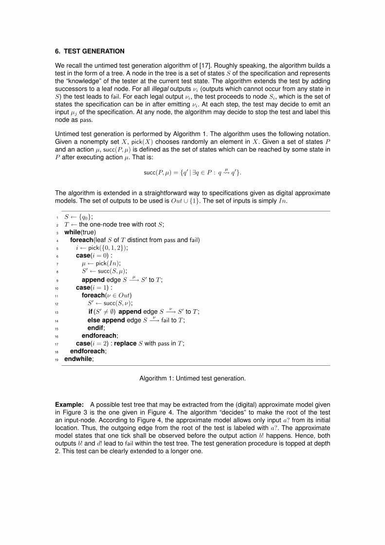
6. TEST GENERATION

We recall the untimed test generation algorithm of [17]. Roughly speaking, the algorithm builds atest in the form of a tree. A node in the tree is a set of states S of the specification and representsthe “knowledge” of the tester at the current test state. The algorithm extends the test by addingsuccessors to a leaf node. For all illegal outputs νi (outputs which cannot occur from any state inS) the test leads to fail. For each legal output νi, the test proceeds to node Si, which is the set ofstates the specification can be in after emitting νi. At each step, the test may decide to emit aninput µj of the specification. At any node, the algorithm may decide to stop the test and label thisnode as pass.

Untimed test generation is performed by Algorithm 1. The algorithm uses the following notation.Given a nonempty set X, pick(X) chooses randomly an element in X. Given a set of states Pand an action µ, succ(P, µ) is defined as the set of states which can be reached by some state inP after executing action µ. That is:

succ(P, µ) = {q′ | ∃q ∈ P : qµ q′}.

The algorithm is extended in a straightforward way to specifications given as digital approximatemodels. The set of outputs to be used is Out ∪ {1}. The set of inputs is simply In.

1 S ← {q0};2 T ← the one-node tree with root S;3 while(true)4 foreach(leaf S of T distinct from pass and fail)5 i← pick({0, 1, 2});6 case(i = 0) :7 µ← pick(In);8 S′ ← succ(S, µ);9 append edge S µ−→ S′ to T ;

10 case(i = 1) :11 foreach(ν ∈ Out)12 S′ ← succ(S, ν);13 if (S′ 6= ∅) append edge S ν−→ S′ to T ;14 else append edge S ν−→ fail to T ;15 endif;16 endforeach;17 case(i = 2) : replace S with pass in T ;18 endforeach;19 endwhile;

Algorithm 1: Untimed test generation.

Example: A possible test tree that may be extracted from the (digital) approximate model givenin Figure 3 is the one given in Figure 4. The algorithm “decides” to make the root of the testan input-node. According to Figure 4, the approximate model allows only input a? from its initiallocation. Thus, the outgoing edge from the root of the test is labeled with a?. The approximatemodel states that one tick shall be observed before the output action b! happens. Hence, bothoutputs b! and d! lead to fail within the test tree. The test generation procedure is topped at depth2. This test can be clearly extended to a longer one.

7. CONCLUSION

We introduced a method for testing duration systems. We proposed a framework for modellingreal-time systems based on Duration Variable Timed Graphs with Inputs and Outputs (DVTG-IO) which extend the timed automaton model. We gave an approximation method based ondigitization techniques. A given DVTG-IO is abstracted into an approximate model. Test treesare then extracted form this approximate model.

REFERENCES

[1] Rajeev Alur, Costas Courcoubetis, and David L. Dill. Model-checking for real-time systems.In LICS, pages 414–425, 1990. 2

[2] Rajeev Alur and David L. Dill. A theory of timed automata. Theor. Comput. Sci., 126(2):183–235, 1994. 1, 2

[3] Henrik C. Bohnenkamp and Axel Belinfante. Timed testing with torx. In FM, pages 173–188,2005. 2

[4] Ahmed Bouajjani, Rachid Echahed, and Riadh Robbana. Verfying invariance properties oftimed systems with duration variables. In FTRTFT, pages 193–210, 1994. 1, 2

[5] Karlis Cerans. Decidability of bisimulation equivalences for parallel timer processes. In CAV,pages 302–315, 1992. 2

[6] Abdeslam En-Nouaary, Rachida Dssouli, Ferhat Khendek, and A. Elqortobi. Timed testcases generation based on state characterization technique. In IEEE Real-Time SystemsSymposium, pages 220–, 1998. 2

[7] Thomas A. Henzinger, Zohar Manna, and Amir Pnueli. What good are digital clocks? InICALP, pages 545–558, 1992. 7

[8] Anders Hessel, Kim Guldstrand Larsen, Brian Nielsen, Paul Pettersson, and Arne Skou.Time-optimal real-time test case generation using uppaal. In FATES, pages 114–130, 2003.2

[9] Anders Hessel and Paul Pettersson. A test case generation algorithm for real-time systems.In QSIC, pages 268–273, 2004. 2

[10] A. Khoumsi. A method for testing the conformance of real time systems. In FTRTFT’02,volume 2469 of LNCS. Springer, 2002. 2

[11] M. Krichen and S. Tripakis. Black-box conformance testing for real-time systems. In 11thInternational SPIN Workshop on Model Checking of Software (SPIN’04), volume 2989 ofLNCS. Springer, 2004. 2, 5

[12] Lotfi Majdoub and Riadh Robbana. Test purpose of duration systems. In MSVVEIS, pages67–75, 2006. 2

[13] M. Mikucionis, K G. Larsen, and B. Nielsen. Online on-the-fly testing of realtime systems. InBasic Research in Computer Science, BRICS Report Series RS-03-49, December 2003. 2

[14] P. Morel. Une algorithmique efficace pour la generation automatique de tests de conformite.PhD thesis, Universite de Rennes, 2000. 2

[15] Riadh Robbana. Verification of duration systems using an approximation approach. J.Comput. Sci. Technol., 18(2):153–162, 2003. 7

[16] Jan Springintveld, Frits W. Vaandrager, and Pedro R. D’Argenio. Testing timed automata.Theor. Comput. Sci., 254(1-2):225–257, 2001. 2

[17] Jan Tretmans. Testing concurrent systems: A formal approach. In CONCUR, pages 46–65,1999. 2, 5, 11, 13