TERRALOC MK6 v2 och Mk8 Reference manual Windows XP ... · TERRALOC Seismic System Reference Manual...

TERRALOC

Seismic System

Reference Manual for ABEM Terraloc® Mk6 v2 and Mk8 with ABEM SeisTW for Windows XP ®

2009-05-19

I

COPYRIGHT

Copyright © 2009 by ABEM Instrument AB, all rights reserved.

TRADEMARKS

TERRALOC® is a registered trademark of ABEM Instrument AB.

IBM®and PC/AT® are registered trademarks of International Business Machines Corporation.

Microsoft® and Windows® are registered trademarks of Microsoft Corporation. All other trademarks belong to their respective holder.

General information

Information in this manual is subject to change without notice and constitutes no commitment by ABEM Instrument AB.

ABEM Instrument AB takes no responsibility for errors in this manual or problems that may arise from the use of this material.

Contact information

Address:

ABEM Instrument AB Allén 1 17266 Sundbyberg Sweden

Phone: +46 8 564 88 300

Fax: +46 8 28 11 09

Website: www.abem.se

Email: [email protected]

[email protected]

II

Contents 1. GET TO KNOW YOUR TERRALOC® .....................................................................................1

1.1 WELCOME TO REFRACTION, REFLECTION AND TOMOGRAPHY .............................................1 1.2 THE POWERFUL FEATURES OF THE ABEM TERRALOC MK6 V2 ............................................1 1.3 THE POWERFUL FEATURES OF THE ABEM TERRALOC MK8 .................................................2 1.4 REGISTER YOUR WARRANTY AND SOFTWARE ......................................................................2 1.5 DID YOUR TERRALOC ARRIVE COMPLETE AND UNDAMAGED ?........................................3 1.6 TAKE TIME TO READ THE TECHNICAL DOCUMENTATION .....................................................4 1.7 SOFTWARE.............................................................................................................................4 1.8 WHAT IS SEISTW ?................................................................................................................4 1.9 TECHNICAL SPECIFICATION ABEM TERRALOC MK6 V2 ...................................................5 1.10 TECHNICAL SPECIFICATION ABEM TERRALOC MK8 ........................................................6

2. THE FIELD UNIT AND PROGRAM CONVENTIONS..........................................................7

2.1 EXTERNAL CONNECTIONS TERRALOC MK6 V2..................................................................7 2.2 EXTERNAL CONNECTIONS TERRALOC MK8.......................................................................8 2.3 MEMORY CARD READER TERRALOC MK8..........................................................................9 2.4 CONVENTIONS USED IN THE REFERENCE MANUAL .............................................................10 2.5 BUILT IN KEYBOARD ...........................................................................................................10

2.5.1 Selecting Menu Commands .............................................................................................11 2.6 KEY DESCRIPTIONS .............................................................................................................12

2.6.1 General.............................................................................................................................12 2.6.2 Acquisition mode .............................................................................................................13 2.6.3 Record/Trace/Frequency view .........................................................................................13 2.6.4 Velocity Analyzer ............................................................................................................15 2.6.5 Noise monitor...................................................................................................................16

2.7 EXTERNAL PC-AT KEYBOARD............................................................................................17 2.8 INTERCONNECTING TWO OR MORE TERRALOC´S.............................................................18

3. QUICK START...........................................................................................................................21

3.1 MAIN GRAPHICAL USER INTERFACE (GUI) COMPONENTS...................................................23 3.1.1 Title bar............................................................................................................................23 3.1.2 Menu bar ..........................................................................................................................23 3.1.3 Tool bar............................................................................................................................23 3.1.4 Record view .....................................................................................................................23 3.1.5 Trace view........................................................................................................................24 3.1.6 Record status bar..............................................................................................................24 3.1.7 Application status bar.......................................................................................................25

4. BASIC OPERATION .................................................................................................................27

4.1 START A MEASUREMENT......................................................................................................27 4.2 ARMING AND TRIGGING ......................................................................................................27 4.3 SAVE AND UPDATE ..............................................................................................................27 4.4 TRANSFER DATA .................................................................................................................28

4.4.1 File transfers using the Ethernet port ...............................................................................28 4.4.2 Other ways to transfer data ..............................................................................................28

4.5 ACQUISITION MODES ..........................................................................................................29 Standard ...........................................................................................................................29 Roll-along ........................................................................................................................29 Optimum offset ................................................................................................................29

5. USER INTERFACE ...................................................................................................................31

5.1 QUICK MENU.......................................................................................................................31 5.2 CONTEXT MENU ..................................................................................................................32 5.3 ABOUT.................................................................................................................................33 5.4 ACQUISITION SETUP ............................................................................................................34

5.4.1 Sampling interval .............................................................................................................34

III

5.4.2 No of samples ..................................................................................................................34 5.4.3 Pre-trig/delay....................................................................................................................35 5.4.4 No of stacks......................................................................................................................35 5.4.5 Stack mode.......................................................................................................................35

Fast stack ......................................................................................................................35 Auto stack.....................................................................................................................35 Preview.........................................................................................................................35 Single stack...................................................................................................................35

5.4.6 Re-arm mode....................................................................................................................36 5.5 TRIG SETUP .........................................................................................................................36

5.5.1 Trig input mode................................................................................................................36 Analog ..........................................................................................................................36 Make/break ...................................................................................................................36 TTL rising edge ............................................................................................................36 TTL falling edge ...........................................................................................................36

5.5.2 Trig input level.................................................................................................................37 5.5.3 External Arm Input ..........................................................................................................38

External arm input mode ..............................................................................................38 5.5.4 Arm/Trig Output ..............................................................................................................38

External trig out mode ..................................................................................................38 External arm out mode..................................................................................................38 Ext. arm verify..............................................................................................................38 Verify timeout...............................................................................................................38

5.6 NOISE MONITOR SETUP .......................................................................................................39 5.6.1 Noise monitor status.........................................................................................................39 5.6.2 Damping...........................................................................................................................39 5.6.3 Threshold level.................................................................................................................39 5.6.4 Show noise .......................................................................................................................39

5.7 GEOPHONE TEST..................................................................................................................40 5.8 ACQUISITION FILTER SETUP ................................................................................................40

5.8.1 Notch filter .......................................................................................................................40 5.8.2 Analog low-cut filter ........................................................................................................40

Status ............................................................................................................................41 Slope .............................................................................................................................41 Cutoff freq. ...................................................................................................................41

5.9 RECEIVER SPREAD DIALOG .................................................................................................42 5.9.1 Channel ............................................................................................................................42 5.9.2 Polarity.............................................................................................................................42 5.9.3 Stack on............................................................................................................................43 5.9.4 Trace on ...........................................................................................................................43

5.10 LAYOUT GEOMETRY DIALOG ..............................................................................................44 5.10.1 Source location.................................................................................................................44 5.10.2 Receiver locations ............................................................................................................44 5.10.3 Move-ups .........................................................................................................................45

Units .............................................................................................................................45 Source type (*)..............................................................................................................45 Receiver type (*) ..........................................................................................................45 Ref. channel ..................................................................................................................45

5.10.4 Roll-along ........................................................................................................................45 Roll-along reverse direction .........................................................................................45 First trace ......................................................................................................................45 Length...........................................................................................................................45 Step size........................................................................................................................45

5.11 LAYOUT HELPER .................................................................................................................46 5.11.1 Layout start ......................................................................................................................46 5.11.2 Layout end .......................................................................................................................46 5.11.3 Receiver separation ..........................................................................................................46

5.12 HEADER INFO DIALOG.........................................................................................................47 Job ID ...........................................................................................................................47 Line ID..........................................................................................................................47

IV

Client ............................................................................................................................47 Company.......................................................................................................................47 Observer .......................................................................................................................47 Note ..............................................................................................................................47

5.13 VIEW OPTIONS.....................................................................................................................48 5.13.1 View mode .......................................................................................................................48

Enhanced ......................................................................................................................48 Normalize .....................................................................................................................48 AGC..............................................................................................................................48 Hyperbolic ....................................................................................................................48

5.13.2 Trace style ........................................................................................................................49 VAR+ ...........................................................................................................................49 VAR- ............................................................................................................................49 Wiggle ..........................................................................................................................49 Dotted ...........................................................................................................................49

5.13.3 Time compression ............................................................................................................49 5.13.4 Scale factor.......................................................................................................................49 5.13.5 Trace clip .........................................................................................................................49 5.13.6 Remove DC offset............................................................................................................49 5.13.7 Show tic lines ...................................................................................................................49 5.13.8 Normalize.........................................................................................................................49

Global scaling ...............................................................................................................49 5.13.9 AGC .................................................................................................................................49

AGC window................................................................................................................49 5.13.10 Enhanced..........................................................................................................................50

Average.........................................................................................................................50 Attenuation ...................................................................................................................50

5.13.11 Hyperbolic........................................................................................................................50 Logarithmic ..................................................................................................................50 Linear range..................................................................................................................50

5.13.12 Frequency analysis ...........................................................................................................50 Windowing function .....................................................................................................50 Max frequency..............................................................................................................50 Dynamic range..............................................................................................................50

5.13.13 Velocity analyzer .............................................................................................................51 5.14 OPTIMIZING .........................................................................................................................52

5.14.1 Optimize For Speed .........................................................................................................52 5.14.2 Optimize For Security......................................................................................................52

5.15 DATA SAFETY......................................................................................................................52

6. PROCESS ....................................................................................................................................53

6.1 FIRST BREAKS......................................................................................................................53 6.1.1 Auto .................................................................................................................................53 6.1.2 Clear.................................................................................................................................53 6.1.3 Save..................................................................................................................................53 6.1.4 Load .................................................................................................................................53

6.2 FIR FILTER ..........................................................................................................................54 6.2.1 Filter type .........................................................................................................................54 6.2.2 Windowing function ........................................................................................................54 6.2.3 Cut-off frequencies ..........................................................................................................55 6.2.4 Filter length......................................................................................................................55

6.3 CROSS CORRELATE ..............................................................................................................55 6.4 MOVING AVERAGE ..............................................................................................................57

7. TRIGGERING METHODS.......................................................................................................59

7.1 MAKE/BREAK SWITCH INPUT ..............................................................................................59 7.2 USING THE TRIGGER COIL...................................................................................................59 7.3 RADIO TRIGGERING .............................................................................................................59

V

8. TROUBLESHOOTING .............................................................................................................61

8.1 GENERAL SEISTW PROGRAM PROBLEMS.............................................................................61 8.1.1 The Program Does Not Start ............................................................................................61

8.2 DATA ACQUISITION PROBLEMS ...........................................................................................61 8.2.1 TERRALOC Only Waits For Confirmation When Arming.............................................61 8.2.2 Dead Channels .................................................................................................................61 8.2.3 Data Is Not Displayed ......................................................................................................61 8.2.4 Large Offset .....................................................................................................................61 8.2.5 Incorrect Channel Order...................................................................................................61

8.3 TRIGGER PROBLEMS ............................................................................................................62 8.3.1 Triggering Too Late (Or Early)........................................................................................62 8.3.2 Spurious Triggering .........................................................................................................62 8.3.3 Unable To Trigger............................................................................................................62 8.3.4 Triggering Immediately When Arming............................................................................62

9. APPENDIX A..............................................................................................................................63

9.1 SOFTWARE INSTALLATION ..................................................................................................63 9.2 INSTALL PROCEDURE FOR SEISTW ......................................................................................63 9.3 BOOT PREPARATIONS...........................................................................................................64 9.4 TERRALOC MK6 / MK8 DRIVER .......................................................................................65 9.5 FIRST ARRIVALS FILE FORMAT (*.FIR)...............................................................................66

9.5.1 General.............................................................................................................................66 9.5.2 Description.......................................................................................................................66

10. APPENDIX B ..............................................................................................................................69

10.1 CONNECTORS ......................................................................................................................69 10.1.1 Seismic Input Connectors ................................................................................................69 10.1.2 Power Connector..............................................................................................................71 10.1.3 TTL Arm/Trig Connector ................................................................................................71

11. APPENDIX C..............................................................................................................................73

11.1 SEISMIC METHODS ............................................................................................................73 11.1.1 Refraction.........................................................................................................................73 11.1.2 Reflection.........................................................................................................................73 11.1.3 Optimum Offset ...............................................................................................................74 11.1.4 Tomography.....................................................................................................................74 11.1.5 VSP ..................................................................................................................................74 11.1.6 Vibroseis ..........................................................................................................................74

12. BIBLIOGRAPHY.......................................................................................................................75

VI

List Of Figures Figure 2-1 TERRALOC Mk6 v2 rear panel. ...................................................................................... 7 Figure 2-2 TERRALOC Mk8 rear panel. .......................................................................................... 8 Figure 2-3 TERRALOC Mk8 memory card reader ............................................................................ 9 Figure 2-4 TERRALOC Mk6 v2 / Mk8 built in keyboard .............................................................. 10 Figure 2-5 The TTL Arm/Trig connector .......................................................................................... 18 Figure 2-6 96-channel record, made using four synchronized TERRALOC Mk6 ............................ 18 Figure 2-7 Shows how four TERRALOC´s are used creating a 96 channel system.......................... 19 Figure 3-1 Main graphical user interface........................................................................................... 23 Figure 5-1 The Quick menu............................................................................................................... 31 Figure 5-2 Context menu ................................................................................................................... 32 Figure 5-3 The About dialog ............................................................................................................. 33 Figure 5-4 Acquisition Setup menu ................................................................................................... 34 Figure 5-5 The Trig Setup menu........................................................................................................ 36 Figure 5-6 Trig signal from a geophone and the trig event................................................................ 37 Figure 5-7 The Noise Monitor Setup menu ....................................................................................... 39 Figure 5-8 The Acquisition Filter Setup Menu.................................................................................. 40 Figure 5-9 Receiver Spread Dialog Menu ......................................................................................... 42 Figure 5-10 Layout Geometry Dialog Menu ....................................................................................... 44 Figure 5-11 The Layout Helper menu ................................................................................................. 46 Figure 5-12 The Header Info Dialog menu.......................................................................................... 47 Figure 5-13 The View Options menu .................................................................................................. 48 Figure 5-14 The Velocity Analyzer menu ........................................................................................... 51 Figure 6-1 First breaks menu with the Save first arrival times dialog ............................................... 53 Figure 6-2 FIR Filter menu................................................................................................................ 54 Figure 6-3 Cross correlate menu with the reference trace selection dialog ....................................... 55 Figure 6-4 Raw data........................................................................................................................... 56 Figure 6-5 After cross correlation...................................................................................................... 56 Figure 6-6 The Moving Average menu ............................................................................................. 57 Figure 9-1 SeisTW Setup - Select Components................................................................................. 63 Figure 9-2 SeisTW Setup – Terraloc Configuration.......................................................................... 64 Figure 10-1 Seismic input connector 24 channel TERRALOC........................................................... 69 Figure 10-2 Seismic input connector 48 channel TERRALOC........................................................... 70 Figure 10-3 Power connector............................................................................................................... 71 Figure 10-4 TTL Arm/Trig connector ................................................................................................. 71

List of Tables Table 2-1 Conventions used in the reference manual....................................................................... 10 Table 2-2 The names used in this manual ........................................................................................ 11 Table 2-3 General key commands.................................................................................................... 12 Table 2-4 Key commands - Acquisition mode ................................................................................. 13 Table 2-5 Key commands - Record/Trace/Frequency view ............................................................. 13 Table 2-6 Key commands - Velocity analyzer ................................................................................. 15 Table 2-7 Key commands - Noise monitor ...................................................................................... 16 Table 2-8 Keyboard mapping PC/Internal........................................................................................ 17 Table 3-1 Record status bar.............................................................................................................. 24 Table 3-2 Record status bar.............................................................................................................. 25 Table 3-3 Instrument state ................................................................................................................ 25 Table 5-1 Delay times depends on the sampling interval ................................................................. 35 Table 5-2 Available 3 dB cutoff frequencies (in Hz) ....................................................................... 41 Table 5-3 Key commands - Channel mapping ................................................................................. 42 Table 5-4 Key commands - Polarity................................................................................................. 43 Table 5-5 Key commands - Stack on ............................................................................................... 43 Table 5-6 Key commands - Trace on ............................................................................................... 43

1. Get to Know Your Terraloc

1

1. GET TO KNOW YOUR TERRALOC®

1.1 Welcome To Refraction, Reflection And Tomography

Welcome to the ABEM TERRALOC® Mk6 v2 and MK8, the multi-channel digital seismograph for cost-effective refraction and high-resolution reflection surveys, tomography, vibration measurements, and more, anywhere in the world in all weather conditions.

The basic TERRALOC is a self-contained multi-channel seismograph with internal PC-compatible computer ,a hard disk, and a daylight visible TFT color display with VGA resolution. Operating power comes from any external battery pack or power source that delivers from 10 - 30 volts DC. Typically this means a re-chargeable battery pack, a car (or truck) battery, or AC/DC power supply.

TERRALOC Mk6 v2 has a harddisk with a size of at least 10 GB and a 3 1/2 in. 1.44 MB floppy disk, it connects as standard to a printer, PS/2 mouse, external PS/2 keyboard, external VGA monitor, it also offers serial and Ethernet connectivity.

TERRALOC Mk8 has a harddisk with a size of at least 80 GB and a built in memory card reader, it has 3 USB 2.0 ports, Ethernet and VGA monitor port.

With more than 24 channels installed, TERRALOC comes in a slightly bigger and heavier casing.

After a survey you may process data stored on the internal hard disk or on a floppy disk either using TERRALOC´s internal PC or an external computer. Large amounts of data can be transferred between the TERRALOC and an external PC using the built in Ethernet port in the TERRALOC. For filtering and basic processing you can use the TERRALOC´s internal software called SeisTW which is the software developed by ABEM that controls the TERRALOC´s functions. Third party software packages for seismic data processing can be run directly on the TERRALOC. Please ask your authorized ABEM Distributor for details about seismic interpretation and processing packages that are available.

Your TERRALOC was carefully checked at all stages of production. It was thoroughly tested before being approved for delivery. If you handle and maintain it according to the instructions in the technical documentation, you will get many years of satisfactory service from it.

1.2 The Powerful Features of the ABEM Terraloc Mk6 v2

Among the powerful features you’ll find in ABEM TERRALOC Mk6 v2 are:

• Ethernet port for fast transfers of data and networking capabilities

• Daylight visible color TFT display

• Excellent resolution thanks to an 18 bit ADC (analog/digital converter) and 3 bit IFP (instantaneous floating point) amplifier

• In-field quality control of measurements thanks to geophone tests, noise monitoring, and a wide choice of single- or multi-trace view modes

• Excellent results for tomography and high resolution seismics thanks to selectable sampling rates from 25 µs to 2 ms in seven steps

• Full on-screen display of recorded traces with software roll-along, automatic pick of first arrivals, list of first arrival times, velocity calculation, frequency analysis of single traces.


2

1.3 The Powerful Features of the ABEM Terraloc Mk8

Among the powerful features you’ll find in ABEM TERRALOC Mk8 are:

• SeisTW for Windows XP, ABEM developed measurement software (Included and factory installed)

• 3 USB ports for connecting external accessories such as USB CD/DVD, USB memory sticks, keyboard, mouse etc.

• Memory card reader for backup when in the field and for transfers of data/files ( SD, Compact flash and Memory stick pro duo cards can be inserted and is protected by cover in field use).

• Ethernet port for fast transfers of data and networking capabilities

• Daylight visible color TFT display

• Excellent resolution thanks to an 18 bit ADC (analog/digital converter) and 3 bit IFP (instantaneous floating point) amplifier

• In-field quality control of measurements thanks to geophone tests, noise monitoring, and a wide choice of single- or multi-trace view modes

• Excellent results for tomography and high resolution seismics thanks to selectable sampling rates from 25 µs to 2 ms in seven steps

• Full on-screen display of recorded traces with software roll-along, automatic pick of first arrivals, list of first arrival times, velocity calculation, frequency analysis of single traces.

1.4 Register Your Warranty and Software

Fill in and mail your Warranty Card without delay. When you are registered with ABEM, you'll get information about product updates, operating and service tips, special offers, etc. So take a minute now, fill in the card, and mail it. Your TERRALOC is covered by the ABEM Worldwide Warranty.

This means the equipment is free from defects due to material or faulty workmanship. The warranty covers servicing and adjusting of any defective parts excluding fuses, and batteries provided the TERRALOC is returned, freight and insurance paid, to ABEM. If ABEM finds that the cause of fault or defect is due to misuse or abnormal operating conditions, then repairs will be invoiced at cost. ABEM assumes no responsibility for steps that are either taken or not taken as the result of decisions based on the results of measurements taken with TERRALOC or calculations based on software delivered by ABEM. The warranty is valid for twelve (12) months from date of Bill of Lading or other delivery document issued to the original purchaser. ABEM liability under this warranty is limited in accordance with terms outlined in, the General Conditions for the Supply of Mechanical, Electric and Electronic products, prepared by ORGALIME, Brussels, August 2000.


3

1.5 Did Your TERRALOC Arrive Complete And Undamaged ?

Your TERRALOC arrives in a transport box. Open it and unpack all items carefully. Check contents against the invoice. Check box for transport or handling damage.

A standard ABEM TERRALOC Mk8 basic system includes the following

1 TERRALOC field unit with a number of channels as shown on the packing list

1 Accessories and tools kit comprising

1 Tool bag

10 fuses 2.4 Amp "slow"

1 Cable for external battery, with connector and crocodile clips

1 Cable for office power supply: mains cable with appropriate plug, interconnect cable with car lighter socket adapter

2 2 m connection cables (for trigger coil)

1 Insulating tape roll

1 Engineer pliers

1 Pair of cutting nippers

1 Hex wrench 4 mm

1 Hex wrench 5 mm

1 Screwdriver 2.5 mm x 50 mm

1 Phillips screwdriver

1 Trigger coil

1 Documentation kit, comprising

2 TERRALOC Reference manuals

1 Windows XP license (CD)

1 SD memory card

1 Warranty registration card

1 Trigger cable, 250m, on reel

Optional item / not included: Office power supply, 115/230 V

Check that you have received all items shown on the invoice; check also that they are externally undamaged. If you ordered optional equipment, check the invoice for details and compare with your original order.

File any claim for shipping damage with the carrier immediately on discovery and before using the TERRALOC. Send a copy of your claim or damage report to ABEM or to your authorized ABEM Distributor. If it is a question of short shipment you must make a claim in writing to ABEM within 14 days of your receipt of shipment. Please state the original ABEM Invoice Number and the TERRALOC serial number in all correspondence with ABEM or your authorized ABEM Distributor.

You should keep and store all original packing material for later use, for example, to send the TERRALOC for service. If you do not have access to original packing material, then pack your TERRALOC in a robust box large enough to allow 80 mm of shock absorbing material to be placed all around the equipment top, bottom, and all sides. Never use shredded fibre, paper or wood wool these materials pack down in transport and the equipment may move around inside the box. If you have to return your TERRALOC to ABEM or its authorized distributor, please ask for shipping instructions before despatch.


4

1.6 Take Time to Read The Technical Documentation

To ensure you get optimum results with ABEM TERRALOC Mk6 v2 and Mk8, please take time to read the reference manual thoroughly. You should also look through the Manual to become familiar with its layout and contents. If you should, for any reason, have difficulties in operating ABEM TERRALOC Mk6 v2 / Mk8 or in getting satisfactory seismic survey results, please contact your authorised ABEM distributor. ABEM always listens to end-user comments about their experience with ABEM products. So please send occasional reports on field usage as well as your ideas on how the TERRALOC and its technical documentation could be improved to help you do an even better job of seismic surveying.

1.7 Software

TERRALOC Mk6 v2 and Mk8 is delivered with all necessary software installed at the factory,. However, SeisTW was not installed at the factory in the Mk6 v2 only in the Mk8. If you have a Terraloc Mk6 v2 and have not received the SeisTW software please contact ABEM. If the software needs to be updated, or re-installed, the procedure is described in this reference manual.(Appendix A)

1.8 What is SeisTW ?

SeisTW which stands for Seismograph Terraloc Windows is a Windows XP application that is used to control the TERRALOC Mk6 v2 and Mk8 seismic system. It can also be installed on any PC running Windows XP and used to view and manage seismic records. However, when installed on a PC in this way, all functions accessing the TERRALOC Mk6 v2 / Mk8 API, will be disabled.

SeisTW is included and factory installed in all TERRALOC Mk8 instruments, SeisTW can also be used in all TERRALOC Mk6 v2 instruments, check with ABEM to make sure your TERRALOC Mk6 is compatible if you would like to install SeisTW.


5

1.9 Technical Specification ABEM TERRALOC Mk6 v2 Up-hole channel Channel 12 or 24, redirectable to a separate connector. (With more than 24 channels,

channels 24 and 48 are redirectable).

Sampling rates 25, 50, 100, 250, 500, 1000, 2000 µs.

Record length Selectable from 3.2 ms to 32.7 s equivalent to 128, 256, 512, 1024, 2048, 4096, 8192 or 16384 samples.

Maximum number of stacks 256

Pre-trig recording Selectable, 0-100 % of record length.

Delay time Max delay time is related to the sampling interval. For example selectable, from 0-0.8 s at 25 µs sampling interval to 0-131 s at 2000 µs sampling interval.

First arrivals picking Automatic or manual. Picked first arrivals can be saved to disk.

Trigger inputs Make/break (=switcher), Analog or TTL.

A/D converter resolution 18 bits + 3 bit IFP (= 21 bits)

Dynamic range 126 dB (theoretical)

Min/Max input signal Min: ± 0.24 µV. Max: ± 250 mV.

Frequency range 2 - 4000 Hz

High pass (low-cut) filter Selectable, 12 dB/octave 12-192 Hz in 16 steps or 24 dB/octave 15-240 Hz in 16 steps.

Notch filter 50 or 60 Hz. Specify when ordering for factory installation and calibration.

Anti-aliasing Automatically set according to sampling frequency.

Processor AMD GX1-300

Memory 256 MB RAM

Data storage At least 10 GB internal hard disk (depending on year produced) and 1.44 MB floppy disk drive 3.5 inch.

Display 8,4 inch daylight visible backlighted color TFT display, VGA resolution (640x480 pixels).

Connectivity Parallel (Centronics), serial (RS-232) ,PS/2 Mouse , PS/2 external keyboard, Ethernet and external monitor (VGA),

Power 10-30 V DC external battery or office power supply.

Maximum power consumption 15 W (sleep mode), 40 W (operating mode).

Operating temperature 5° C to 50° C. If unit is at normal room temperature (from being kept indoors) when switched on, it generates enough internal heat for field work at temperatures down to -5° C.

Storage temperature - 40° C to +80° C.

Casing Waterproof, rugged cast aluminium.

Dimensions 400 x 250 x 300 mm (24-channel casing).

Weight 16 kg (24-channel casing).


6

1.10 Technical Specification ABEM TERRALOC Mk8 Up-hole channel Channel 12 or 24, redirectable to a separate connector. (With more than 24 channels,

channels 24 and 48 are redirectable).

Sampling rates 25, 50, 100, 250, 500, 1000, 2000 µs.

Record length Selectable from 3.2 ms to 32.7 s equivalent to 128, 256, 512, 1024, 2048, 4096, 8192 or 16384 samples.

Maximum number of stacks 256

Pre-trig recording Selectable, 0-100 % of record length.

Delay time Max delay time is related to the sampling interval. For example selectable, from 0-0.8 s at 25 µs sampling interval to 0-131 s at 2000 µs sampling interval.

First arrivals picking Automatic or manual. Picked first arrivals can be saved to disk.

Trigger inputs Make/break (=switcher), Analog or TTL.

A/D converter resolution 18 bits + 3 bit IFP (= 21 bits)

Dynamic range 126 dB (theoretical)

Min/Max input signal Min: ± 0.24 µV. Max: ± 250 mV.

Frequency range 2 - 4000 Hz

High pass (low-cut) filter Selectable, 12 dB/octave 12-192 Hz in 16 steps or 24 dB/octave 15-240 Hz in 16 steps.

Notch filter 50 or 60 Hz. Specify when ordering for factory installation and calibration.

Anti-aliasing Automatically set according to sampling frequency.

Processor AMD GX3 LX800

Memory 1GB RAM

Data storage At least 80 GB internal hard disk (depending on year produced) and Memory card reader

Display 8,4 inch daylight visible backlighted color TFT display, VGA resolution (640x480 pixels).

Connectivity USB (3 ports), Ethernet and external monitor (VGA)

Power 10-30 V DC external battery or office power supply.

Maximum power consumption 15 W (sleep mode), 40 W (operating mode).

Operating temperature 5° C to 50° C. If unit is at normal room temperature (from being kept indoors) when switched on, it generates enough internal heat for field work at temperatures down to -5° C.

Storage temperature - 40° C to +80° C.

Casing Waterproof, rugged cast aluminium.

Dimensions 400 x 250 x 300 mm (24-channel casing).

Weight 16 kg (24-channel casing).

2. The Field Unit and Program Conventions

7

2. THE FIELD UNIT AND PROGRAM CONVENTIONS

2.1 External Connections TERRALOC Mk6 v2

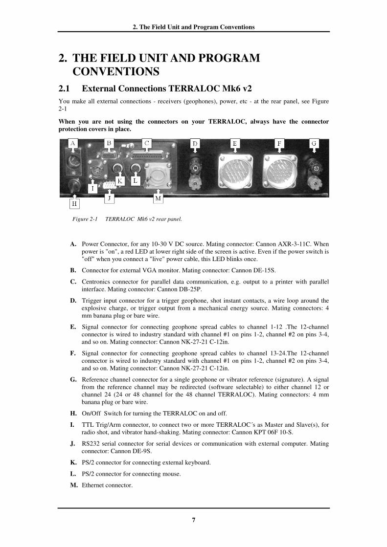
You make all external connections - receivers (geophones), power, etc - at the rear panel, see Figure 2-1

When you are not using the connectors on your TERRALOC, always have the connector protection covers in place.

Figure 2-1 TERRALOC Mk6 v2 rear panel.

A. Power Connector, for any 10-30 V DC source. Mating connector: Cannon AXR-3-11C. When power is "on", a red LED at lower right side of the screen is active. Even if the power switch is "off" when you connect a "live" power cable, this LED blinks once.

B. Connector for external VGA monitor. Mating connector: Cannon DE-15S.

C. Centronics connector for parallel data communication, e.g. output to a printer with parallel interface. Mating connector: Cannon DB-25P.

D. Trigger input connector for a trigger geophone, shot instant contacts, a wire loop around the explosive charge, or trigger output from a mechanical energy source. Mating connectors: 4 mm banana plug or bare wire.

E. Signal connector for connecting geophone spread cables to channel 1-12 .The 12-channel connector is wired to industry standard with channel #1 on pins 1-2, channel #2 on pins 3-4, and so on. Mating connector: Cannon NK-27-21 C-12in.

F. Signal connector for connecting geophone spread cables to channel 13-24.The 12-channel connector is wired to industry standard with channel #1 on pins 1-2, channel #2 on pins 3-4, and so on. Mating connector: Cannon NK-27-21 C-12in.

G. Reference channel connector for a single geophone or vibrator reference (signature). A signal from the reference channel may be redirected (software selectable) to either channel 12 or channel 24 (24 or 48 channel for the 48 channel TERRALOC). Mating connectors: 4 mm banana plug or bare wire.

H. On/Off Switch for turning the TERRALOC on and off.

I. TTL Trig/Arm connector, to connect two or more TERRALOC´s as Master and Slave(s), for radio shot, and vibrator hand-shaking. Mating connector: Cannon KPT 06F 10-S.

J. RS232 serial connector for serial devices or communication with external computer. Mating connector: Cannon DE-9S.

K. PS/2 connector for connecting external keyboard.

L. PS/2 connector for connecting mouse.

M. Ethernet connector.


8

2.2 External Connections TERRALOC Mk8

You make all external connections - receivers (geophones), power, etc - at the rear panel, see Figure 2-12

When you are not using the connectors on your TERRALOC, always have the connector protection covers in place.

Figure 2-2 TERRALOC Mk8 rear panel.

A. Power Connector, for any 10-30 V DC source. Mating connector: Cannon AXR-3-11C. When power is "on", a red LED at lower right side of the screen is active. Even if the power switch is "off" when you connect a "live" power cable, this LED blinks once.

B. Connector for external VGA monitor. Mating connector: Cannon DE-15S.

C. USB 2.0 connector Nr. 2

D. Ethernet connector.

E. Trigger input connector for a trigger geophone, shot instant contacts, a wire loop around the explosive charge, or trigger output from a mechanical energy source. Mating connectors: 4 mm banana plug or bare wire.

F. Signal connector for connecting geophone spread cables to channel 1-12 .The 12-channel connector is wired to industry standard with channel #1 on pins 1-2, channel #2 on pins 3-4, and so on. Mating connector: Cannon NK-27-21 C-12in.

G. Signal connector for connecting geophone spread cables to channel 13-24.The 12-channel connector is wired to industry standard with channel #1 on pins 1-2, channel #2 on pins 3-4, and so on. Mating connector: Cannon NK-27-21 C-12in.

H. Reference channel connector for a single geophone or vibrator reference (signature). A signal from the reference channel may be redirected (software selectable) to either channel 12 or channel 24 (24 or 48 channel for the 48 channel TERRALOC). Mating connectors: 4 mm banana plug or bare wire.

I. On/Off Switch for turning the TERRALOC on and off.

J. TTL Trig/Arm connector, to connect two or more TERRALOC´s as Master and Slave(s), for radio shot, and vibrator hand-shaking. Mating connector: Cannon KPT 06F 10-S.

K. USB 2.0 connector Nr. 1


9

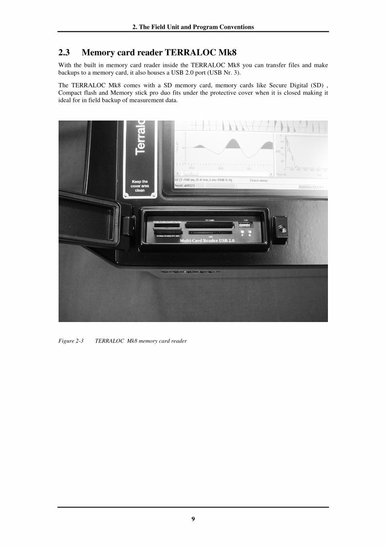
2.3 Memory card reader TERRALOC Mk8

With the built in memory card reader inside the TERRALOC Mk8 you can transfer files and make backups to a memory card, it also houses a USB 2.0 port (USB Nr. 3).

The TERRALOC Mk8 comes with a SD memory card, memory cards like Secure Digital (SD) , Compact flash and Memory stick pro duo fits under the protective cover when it is closed making it ideal for in field backup of measurement data.

Figure 2-3 TERRALOC Mk8 memory card reader


10

2.4 Conventions Used in the Reference Manual

The conventions used in this reference manual are described in table 2-1.

Table 2-1 Conventions used in the reference manual

Ctrl+S Keys, or key combinations on a PC keyboard.

<SAVE> Keys, or key combinations on the TERRALOC built-in keyboard.

File/Save A sequence of selections in the user interface. In this case, first clicking on File in the menu bar, followed by a click on Save.

Quick menu/3 A sequence of selections in the user interface. In this case, pressing <3> (or 3) after accessing the Quick menu.

25, 50, 100, 250, 500, 1000, 2000 Lists available choices in a menu.

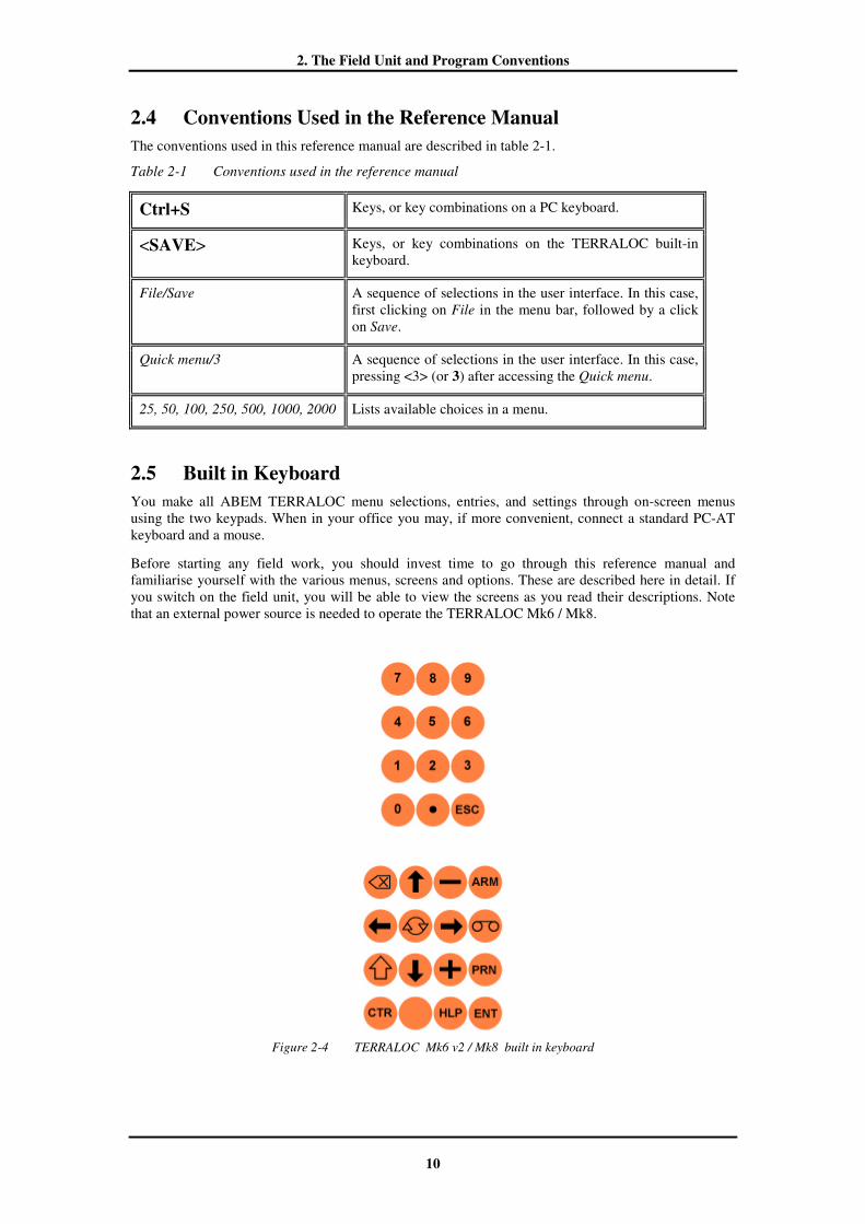
2.5 Built in Keyboard

You make all ABEM TERRALOC menu selections, entries, and settings through on-screen menus using the two keypads. When in your office you may, if more convenient, connect a standard PC-AT keyboard and a mouse.

Before starting any field work, you should invest time to go through this reference manual and familiarise yourself with the various menus, screens and options. These are described here in detail. If you switch on the field unit, you will be able to view the screens as you read their descriptions. Note that an external power source is needed to operate the TERRALOC Mk6 / Mk8.

Figure 2-4 TERRALOC Mk6 v2 / Mk8 built in keyboard


11

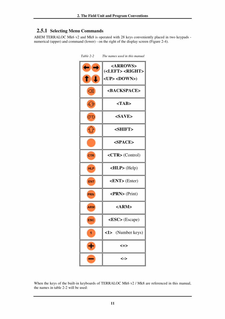
2.5.1 Selecting Menu Commands

ABEM TERRALOC Mk6 v2 and Mk8 is operated with 28 keys conveniently placed in two keypads - numerical (upper) and command (lower) - on the right of the display screen (Figure 2-4).

Table 2-2 The names used in this manual

<ARROWS> (<LEFT> <RIGHT>

<UP> <DOWN>)

<BACKSPACE>

<TAB>

<SAVE>

<SHIFT>

<SPACE>

<CTR> (Control)

<HLP> (Help)

<ENT> (Enter)

<PRN> (Print)

<ARM>

<ESC> (Escape)

<1> (Number keys)

<+>

<->

When the keys of the built-in keyboards of TERRALOC Mk6 v2 / Mk8 are referenced in this manual, the names in table 2-2 will be used:


12

Press <TAB> or <SHIFT> + <TAB> to cycle forward or backward through command line. When a menu is active, it is highlighted with blue colour. To open a drop-down menu press <ENT>. The first command highlights by default; to activate it, press <ENT>. Use <TAB> or <SHIFT> + <TAB> to cycle through all the commands. When a command highlights, press <ENT> to select it. To close a pull-down menu, press <ESC>. In addition to this you can use <ARROWS> to navigate among the pull-down menus.

2.6 Key Descriptions

Below follows a list of the command keys and their functions. Please note that some key functions differ in some menus. When a key has a special function in a menu, it will be explained at the entry for that specific menu.

The tables below only describe special functions of the TERRALOC keys (e.g. opening a context menu), whereas usual meanings, i.e. that it generates a space-character when entering text, are not described.

2.6.1 General

Table 2-3 General key commands

Opens a context menu

Navigates between fields in dialogs

Navigates in reverse direction between fields in dialogs

Opens the Preferences dialog

Saves the current file (prompting for overwrite if the file already exists)

Opens the Save As dialog

Forces a save of the current file (overwriting any existing file)

Opens the Quick menu

Shows/hides the logging window

To select menu bar, see section 4.5 Main Graphical user interface (GUI) Components.

Shows/hides the Trace View and Frequency View.

Shows/hides the toolbar.

Opens the edit source/receivers dialog.

Opens the edit header info dialog.


13

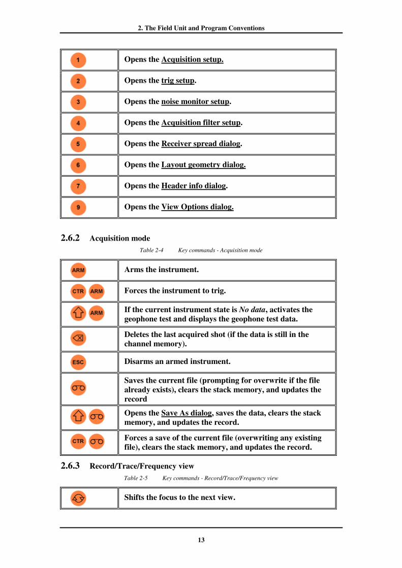
Opens the Acquisition setup.

Opens the trig setup.

Opens the noise monitor setup.

Opens the Acquisition filter setup.

Opens the Receiver spread dialog.

Opens the Layout geometry dialog.

Opens the Header info dialog.

Opens the View Options dialog.

2.6.2 Acquisition mode

Table 2-4 Key commands - Acquisition mode

Arms the instrument.

Forces the instrument to trig.

If the current instrument state is No data, activates the geophone test and displays the geophone test data.

Deletes the last acquired shot (if the data is still in the channel memory).

Disarms an armed instrument.

Saves the current file (prompting for overwrite if the file already exists), clears the stack memory, and updates the record

Opens the Save As dialog, saves the data, clears the stack memory, and updates the record.

Forces a save of the current file (overwriting any existing file), clears the stack memory, and updates the record.

2.6.3 Record/Trace/Frequency view

Table 2-5 Key commands - Record/Trace/Frequency view

Shifts the focus to the next view.


14

Record View: Moves the trace marker to the right (at the end of the record it will wrap around to the beginning). Trace View: Scrolls the trace to the right.

Record View: Moves the trace marker to the left (at the end of the record it will wrap around to the beginning). Trace View: Scrolls the trace to the left

Scrolls the traces down a whole page.

Scrolls the traces up a whole page.

Record view: Scrolls the traces down.

Trace/frequency view: Changes which trace is displayed in view, trace number decreases.

Record view: Scrolls the traces up.

Trace/frequency view: Changes which trace is displayed in view, trace number increases.

Record view: Moves the timeline marker down (increasing time).

Trace view: Moves the timeline marker to the right (increasing time).

Frequency view: Moves the marker to the right (increasing frequency).

If you keep the key pressed, the timeline/marker movement will accelerate.

Record view: Moves the timeline marker up (decreasing time).

Trace view: Moves the timeline marker to the left (decreasing time).

Frequency view: Moves the marker to the left (decreasing frequency).

If you keep the key pressed, the timeline/marker movement will accelerate.

Moves the timeline marker down (increasing time) in large steps.

Moves the timeline marker up (decreasing time) in large steps.


15

Set the first break for the trace selected by the trace marker at the position of the timeline.

Opens the Velocity Analyzer.

Moves the borders of the Trace view.

2.6.4 Velocity Analyzer

Table 2-6 Key commands - Velocity analyzer

Select edit field in velocity analysis bar at top of page.

Moves the velocity marker down (increasing time).

Moves the velocity marker up (decreasing time).

Moves velocity marker to the right.

Moves velocity marker to the left

Moves the free end of the velocity marker down (increases the slope)

Moves the free end of the velocity marker up (decreases the slope)

Moves the free end of the velocity marker to the right.

Moves the free end of the velocity marker to the left.


16

2.6.5 Noise monitor

When the instrument is armed and the noise monitor enabled, all acquisition mode key inputs are valid.

Table 2-7 Key commands - Noise monitor

Increases threshold level. Size of increase depends on amplitude scale of the noise monitor.

Decreases threshold level. Size of decrease depends on amplitude scale of the noise monitor.

When just monitoring the noise (instrument is not armed), pressing <Space> sends a test pulse to the geophones.

Increases the attenuation 6 dB.

Decreases the attenuation 6 dB.


17

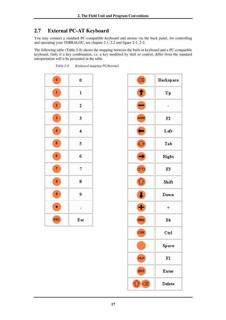
2.7 External PC-AT Keyboard

You may connect a standard PC-compatible keyboard and mouse via the back panel, for controlling and operating your TERRALOC, see chapter 2.1, 2.2 and figure 2-1, 2-2.

The following table (Table 2-8) shows the mapping between the built-in keyboard and a PC-compatible keyboard. Only if a key combination, i.e. a key modified by shift or control, differ from the standard interpretation will it be presented in the table.

Table 2-8 Keyboard mapping PC/Internal


18

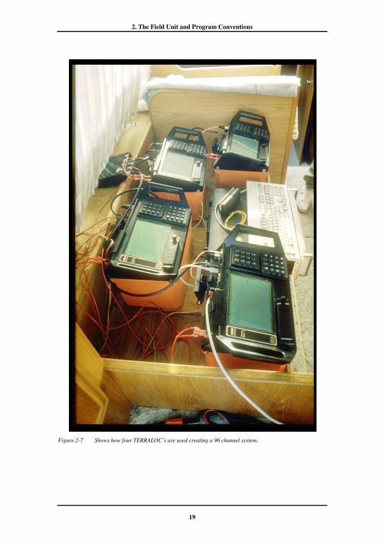
2.8 Interconnecting Two or More TERRALOC´s

Should more channels be needed than can be supplied by the use of a single instrument, it is possible to connect (virtually) any number of TERRALOC´s see figure 2-6 and 2-7. When this is done the Arm, Disarm, and Trigger events are synchronized. Two or more TERRALOC´s may be connected via the TTL Arm/Trig connector , see figure 2-5

TTL stands for Transistor-Transistor-Logic. It is used in connection to digital signals. A digital signal is considered to be either a logical 0 or a logical 1 (hereafter only called 0 and 1). Physically a 0 corresponds to voltage of 0-0.7 V, while a 1 corresponds to a voltage of 2.8-5.0 V. Alternatively, a 0 might be called "low", and a 1 called "high"

An example from a survey where four TERRALOC Mk6 were used to comprise a 96-channel system, see figure 2-6 below.

Figure 2-6 96-channel record, made using four synchronized TERRALOC Mk6

Figure 2-5 The TTL Arm/Trig connector

TTL Arm/Trig connector (Mating side view). A. Trigger Output, B. Arm Input,C. TriggerInput, D. GND (ground), E. No connection, F. Arm Output


19

Figure 2-7 Shows how four TERRALOC´s are used creating a 96 channel system.

3. Quick Start

21

3. QUICK START In this section we will make a measurement of noise. It will give you insight in how easy it is to set your TERRALOC up for operation and you will need no more equipment than the instrument itself and the power supply. Before starting any field work, it’s however wise to invest time to go through and familiarise yourself with the various menus, screens and options. These are described in detail in chapter 4. Should you feel uncertain during any of the steps below, you can press <HLP> to get access to the help screen explaining which key commands does what .

Connect the power supply and switch on the instrument (see figure 2-1 and 2-2)

• Some diagnostic messages show up on the screen during the start up tests and Windows XP is started (if your TERRALOC has dual boot and wasn’t originally delivered with SeisTW you may have to change the Boot.ini to boot Windows XP by default ,this is described in the installation part of this manual chapter 9 (APPENDIX A) ) .

• SeisTW starts automatically.

• Press <CTRL> + <SPACE> to access the Quick Menu. By selecting 1 (New), a dialog where you can choose acquisition mode (Standard, Roll-along, or Optimum offset) by using <ARROW> For the acquisition mode standard, you may also choose number of traces you wish to use.

• Move around the menu by using the <TAB> key, values are selected by using <ARROW> keys and to accept entered values, press <ENT>. <ESC> closes a list without making any selection. In some fields you can type in values directly, using the numerical keys. Before accepting the current settings, make sure you have the stacking mode set to "Auto stack".

• Pressing <ARM> will open an acquisition record using the last active acquisition mode. To verify/change the acquisition settings the easiest way press:

<1> for Acquisition setup (sample interval, number of samples, stacking mode, etc.).

<2> for Trig setup.

<3> for Noise monitor.

<4> for Acquisition (analog) filters.

<5> for Receiver spread (channel assignment, polarity, stack status, trace status). Use <SHIFT> + <+> or <-> to map the channels in forward or reverse direction.

<6> for Layout geometry (source and receiver location, reference channel setup, roll-along settings, etc.).

<7> for Header information (job ID, line ID, notes, etc.). Note that you can only input digits with the built-in keyboard. For letters you need an external PC-compatible keyboard.

<9> for View options (trace style, time compression, scale factor)

3. Quick Start

22

• When you have chosen settings, you should choose working directory. It is wise to check that the measuring files are correctly saved in the right place

• Now press <ARM> again. This arms the instrument and makes it ready to receive a shot The record status bar (bottom of the screen), shows information about the trace and tell you that the instrument is armed

• Press <CTR>+<ARM> to force the instrument to trig. A message "<<< TRIGGERED >>>" is displayed in the Application status bar.)

• Now the data are scaled and displayed in the trace window. To change view options, press <9>.

• If trigging once more by pressing <CTR>+<ARM>, the traces on the screen are replaced with a new set that look a little different. What you see now is the average of the two measurements made so far.

• Press <SAVE> to save the data or press <ESC> to reject and disarm the instrument (a message "Disarming..." shows for a short while).

• When you are finished getting acquainted with the instrument, you may shut off the TERRALOC . Press <CTR>+<SPACE> for the quick menu, select "Power Off" in the sub-menu.

• Now you should have learned a little about how to operate the instrument and navigate between the different menus. Do not be afraid to test different settings and modes. Please refer to the reference manual, should you get stuck in any menu. There is no risk of causing any damage. Should you somehow get problems with the TERRALOC software SeisTW , you can just reinstall it (see chapter 9 APPENDIX A).

3. Quick Start

23

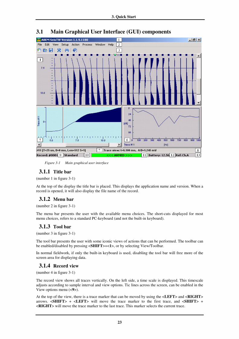
3.1 Main Graphical User Interface (GUI) components

Figure 3-1 Main graphical user interface

3.1.1 Title bar

(number 1 in figure 3-1)

At the top of the display the title bar is placed. This displays the application name and version. When a record is opened, it will also display the file name of the record.

3.1.2 Menu bar


The menu bar presents the user with the available menu choices. The short-cuts displayed for most menu choices, refers to a standard PC-keyboard (and not the built-in keyboard).

3.1.3 Tool bar


The tool bar presents the user with some iconic views of actions that can be performed. The toolbar can be enabled/disabled by pressing <SHIFT>+<1>, or by selecting View/Toolbar.

In normal fieldwork, if only the built-in keyboard is used, disabling the tool bar will free more of the screen area for displaying data.

3.1.4 Record view


The record view shows all traces vertically. On the left side, a time scale is displayed. This timescale adjusts according to sample interval and view options. Tic lines across the screen, can be enabled in the View options menu (<9>).

At the top of the view, there is a trace marker that can be moved by using the <LEFT> and <RIGHT> arrows. <SHIFT> + <LEFT> will move the trace marker to the first trace, and <SHIFT> + <RIGHT> will move the trace marker to the last trace. This marker selects the current trace.

3. Quick Start

24

In acquisition mode, the top of the view also displays the current Stack On status, and polarity. The Stack On is displayed by squares above each trace. If the square is filled the stack for that trace is on, and if the square is open, the same stack is off (will not add acquired data). If negative polarity has been selected for a trace, a minus sign is displayed under the square.

To scroll the view use <UP> and <DOWN>. <SHIFT> + <UP> and <SHIFT> + <DOWN> will scroll the view one page at a time.

Pressing <+> or <-> will move a time line across the view. Some data for the current trace will be displayed in the status field just below the views. Pressing < . > will set a first arrival marker at the location of the time line on the current trace.

Pressing <SHIFT> + <8>, opens the Velocity analyzer.

Pressing <CTR> + <SPACE>, opens context menu with appropriate menu choices.

Press <TAB> to move between views.

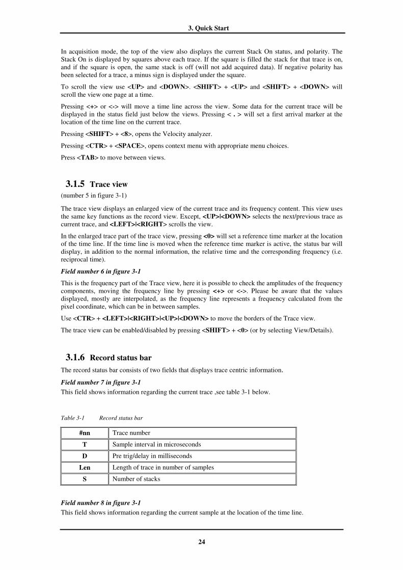
3.1.5 Trace view


The trace view displays an enlarged view of the current trace and its frequency content. This view uses the same key functions as the record view. Except, <UP>|<DOWN> selects the next/previous trace as current trace, and <LEFT>|<RIGHT> scrolls the view.

In the enlarged trace part of the trace view, pressing <0> will set a reference time marker at the location of the time line. If the time line is moved when the reference time marker is active, the status bar will display, in addition to the normal information, the relative time and the corresponding frequency (i.e. reciprocal time).

Field number 6 in figure 3-1

This is the frequency part of the Trace view, here it is possible to check the amplitudes of the frequency components, moving the frequency line by pressing <+> or <->. Please be aware that the values displayed, mostly are interpolated, as the frequency line represents a frequency calculated from the pixel coordinate, which can be in between samples.

Use <CTR> + <LEFT>|<RIGHT>|<UP>|<DOWN> to move the borders of the Trace view.

The trace view can be enabled/disabled by pressing <SHIFT> + <0> (or by selecting View/Details).

3.1.6 Record status bar

The record status bar consists of two fields that displays trace centric information.


This field shows information regarding the current trace ,see table 3-1 below.

Table 3-1 Record status bar

#nn Trace number

T Sample interval in microseconds

D Pre trig/delay in milliseconds

Len Length of trace in number of samples

S Number of stacks


This field shows information regarding the current sample at the location of the time line.

3. Quick Start

25

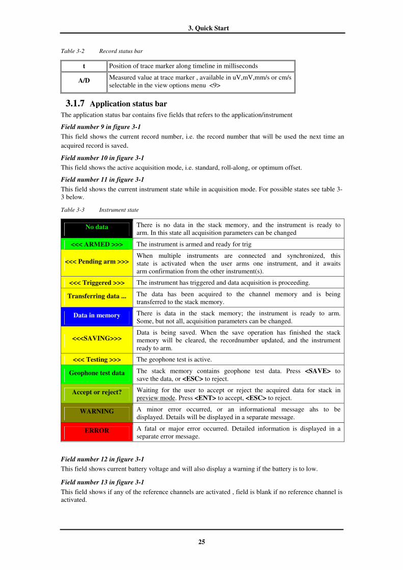
Table 3-2 Record status bar

t Position of trace marker along timeline in milliseconds

A/D Measured value at trace marker , available in uV,mV,mm/s or cm/s selectable in the view options menu <9>

3.1.7 Application status bar

The application status bar contains five fields that refers to the application/instrument


This field shows the current record number, i.e. the record number that will be used the next time an

acquired record is saved.


This field shows the active acquisition mode, i.e. standard, roll-along, or optimum offset.


This field shows the current instrument state while in acquisition mode. For possible states see table 3-3 below.

Table 3-3 Instrument state

No data There is no data in the stack memory, and the instrument is ready to arm. In this state all acquisition parameters can be changed

<<< ARMED >>> The instrument is armed and ready for trig

<<< Pending arm >>> When multiple instruments are connected and synchronized, this state is activated when the user arms one instrument, and it awaits arm confirmation from the other instrument(s).

<<< Triggered >>> The instrument has triggered and data acquisition is proceeding.

Transferring data ... The data has been acquired to the channel memory and is being transferred to the stack memory.

Data in memory There is data in the stack memory; the instrument is ready to arm. Some, but not all, acquisition parameters can be changed.

<<<SAVING>>> Data is being saved. When the save operation has finished the stack memory will be cleared, the recordnumber updated, and the instrument ready to arm.

<<< Testing >>> The geophone test is active.

Geophone test data The stack memory contains geophone test data. Press <SAVE> to save the data, or <ESC> to reject.

Accept or reject? Waiting for the user to accept or reject the acquired data for stack in preview mode. Press <ENT> to accept, <ESC> to reject.

WARNING A minor error occurred, or an informational message ahs to be displayed. Details will be displayed in a separate message.

ERROR A fatal or major error occurred. Detailed information is displayed in a separate error message.


This field shows current battery voltage and will also display a warning if the battery is to low.


This field shows if any of the reference channels are activated , field is blank if no reference channel is activated.

4. Basic Operation

27

4. BASIC OPERATION The preferred way of operating the SeisTW software is by using the built-in keyboard. However, it may be operated using any Windows compatible keyboard and mouse with the correct connectors, PS/2 for Mk6 v2 and USB for Mk8.

4.1 Start a measurement

To start a measurement, either press <ARM>, (F2) or select File/New (Ctrl+N). Selecting New opens a dialog where you can choose acquisition mode (Standard, Roll-along, or Optimum offset). For standard, you may also choose number of traces.

Pressing <ARM> will open an acquisition record using the last active acquisition settings.

When an acquisition record has been created, you should verify the acquisition settings. The easiest way to access these is to press:

• <1> for Acquisition setup (sample interval, number of samples, stacking mode, etc.). • <2> for Trig setup. • <3> for Noise monitor. • <4> for Acquisition (analog) filters. • <5> for Receiver spread (channel assignment, polarity, stack status, trace status). • <6> for Layout geometry (source and receiver location, reference channel setup, roll-along

settings, etc.). • <7> for Header information (job ID, line ID, notes, etc.).

4.2 Arming and Trigging

When all acquisition settings are made, press <ARM> to arm the instrument. The status bar will show the message "<<< ARMED >>>".

The instrument will trig according to the Trig Setup settings. When the instrument triggers, this is indicated in the centre field of the status bar, which will show a message "<<< Triggered >>>". When the data has been acquired, it is transferred from the channel memory to the stack memory. The actual behaviour depends on the active stack mode.

4.3 Save and Update

Press <SAVE> (or F3) when the acquisition of the current record is finished, to save the data. When the data has been saved, the stack memory is cleared, the layout parameters are updated, and the instrument will be ready for the next <ARM>.

It is possible to only save the data (without clearing the stack memory and updating the record) by selecting Save in the Quick menu (<CTR>+<SPACE >) or by pressing Ctrl+S (or File/Save).

4. Basic Operation

28

4.4 Transfer Data

4.4.1 File transfers using the Ethernet port

This is a function of Microsoft Windows XP Professional and not a specific function of ABEM TERRALOC Mk6 v2 / Mk8. Hence, ABEM can not be responsible for any problems that may occur that isn’t associated with the TERRALOC hardware or measurement programs developed by ABEM.

File transfers from your TERRALOC Mk6 v2 / Mk8 to a PC can be done using a simple crossed network cable, this can be done in the field for example using a laptop computer. You will also of course need an external PS/2 keyboard and mouse (supplied with the TERRALOC at delivery) for the TERRALOC.

One way to do this is to set up a small network and allow sharing of a folder which you can copy measurement data to. To do this, go to “network and internet connections” in the control panel and chose “network connections” , in the menu on the left side of the screen select “set up a home or small office network” and follow the wizard.

The network card is factory installed, but before you can install a small network the TERRALOC must be connected to the PC using a crossed network cable (available in most computer stores). Note that using a common network cable will NOT work.

When the wizard has finished, the shared document folder should be automatically shared, you can share a folder of choice if you want to ,just select “Share this folder” in the menu on the left when browsing a folder.

With the TERRALOC Mk6 v2 / Mk8 connected to a PC with the crossed network cable you can then find out the IP number of the TERRALOC writing the “ipconfig” command in the command prompt accessible under “Start menu /All programs / Accessories”.

To access the shared folder in the TERRALOC from the PC, go to “Start / Search / select Computers or people” from the menu on the left and then “A computer on the network”. At this point enter the IP number of the TERRALOC in the Computer name search field and click the search button. You may have to login, but then you should be able to access the files.

Note that there are security issues with sharing folders, never put any sensitive data in a shared folder since it is easy accessible when the TERRALOC is connected to a network or internet. it is also advisable to only allow reading of files and not writing.

Another option is to configure the TERRALOC Mk6 v2 / Mk8 for use in a normal office network, this will not be described in this manual.

4.4.2 Other ways to transfer data

Using the built in floppy drive in the TERRALOC Mk6 v2 may be another option if you only would

like to copy small amounts of data.

TERRALOC Mk8 has built in USB 2.0 ports for fast and easy transfer to a USB memory, it also has a built in memory card reader which is compatible with a number of different types of memory cards including Secure digital (SD), Compact flash and Memory stick cards.

4. Basic Operation

29

4.5 Acquisition Modes

By selecting New under the Quick Menu (<CTR>+<SPACE>), or by pressing Ctrl+N, it is possible to select which acquisition mode to use. The following acquisition modes are available

• Standard

• Roll-along

• Optimum offset

Standard

In this mode all acquisition is performed according to the current settings. The only automatic actions are clearing the stack memory and updating the record after a save & update operation.

Roll-along

When pressing first <ARM>, a new record is created containing the number of traces defined by the Roll-along start/end parameters in the Layout Geometry Dialog.

Pressing <SAVE> will cause the record to be saved and the roll-along parameters to be updated according to the Roll-along step size as defined in the Layout Geometry Dialog. How the Roll-along parameters are updated is determined by the Roll-along reverse direction check box.

Optimum offset

When a record is created in the optimum offset acquisition mode, it will initially have only the first trace's stack enabled. Besides, only the currently active trace and traces containing data will be visible. When the data for the currently active trace has been acquired, the user can press <SAVE>, which will advance the active trace one trace. Pressing <SAVE> when the last trace is active will save and update the record.

It is still possible for the user to modify acquisition parameters, including receiver spread parameters, but be careful. Modifying receiver spread parameters, may lead to acquiring data on a trace that already contains data, but should not be updated.

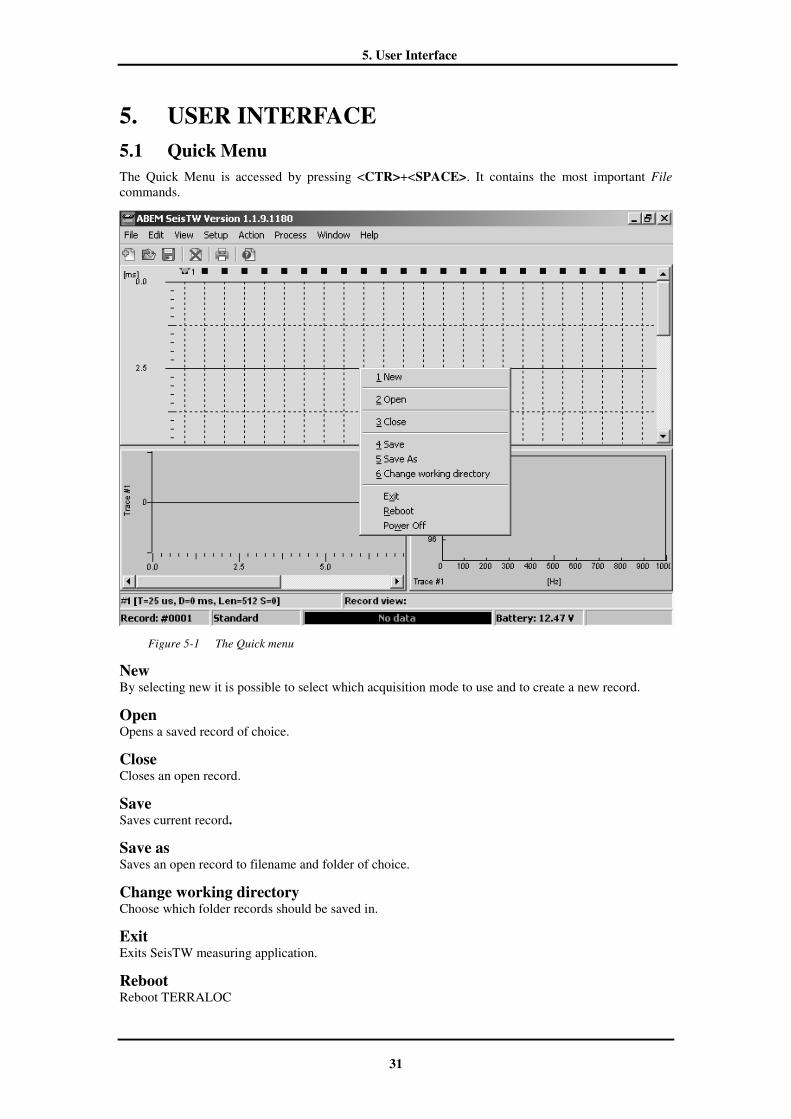
5. User Interface

31

5. USER INTERFACE

5.1 Quick Menu

The Quick Menu is accessed by pressing <CTR>+<SPACE>. It contains the most important File

commands.

Figure 5-1 The Quick menu

New By selecting new it is possible to select which acquisition mode to use and to create a new record.

Open Opens a saved record of choice.

Close Closes an open record.

Save Saves current record.

Save as Saves an open record to filename and folder of choice.

Change working directory Choose which folder records should be saved in.

Exit Exits SeisTW measuring application.

Reboot Reboot TERRALOC

5. User Interface

32

Power off Power off TERRALOC

5.2 Context Menu

The Context Menu is accessed by pressing <SPACE> when in acquisition mode, observe that all selections will not be present if no record has been made. See also chapter 6 Process.

Figure 5-2 Context menu

First breaks

Access the first breaks sub menu.

Velocity Analyzer

Activates the Velocity analyzer.

FIR filter

Access the FIR filter dialog.

Moving average filter

Access the Moving average dialog.

Unfilter data

Discards any processing results and reads back the original data from disk.

Cross correlate

Performs cross correlation of the data.

View options

Access the View options menu.

5. User Interface

33

5.3 About

The About dialog is accessed by pressing <SHIFT>+<HLP> (or Shift + F1). The About dialog displays information about instrument, serial number software versions etc. The most important

information is the API and Driver version numbers. These two numbers have to be identical.

Figure 5-3 The About dialog

5. User Interface

34

5.4 Acquisition Setup

The Acquisition Setup menu is accessed by pressing <1> when in acquisition mode. Note that there is a possibility to save/load settings and also return to the default settings by using the appropriate buttons present in the acquisition setup menu .

Figure 5-4 Acquisition Setup menu

5.4.1 Sampling interval

The sample interval is in microseconds. Available sample intervals are: 25, 50, 100, 250, 500,

1000,2000 microseconds.

You may select record length from short (3.2 ms) to long (32 seconds) depending on your choice of sampling interval and number of samples to be recorded.

Record length = ‘Sampling interval’ x ‘Number of samples’.

If you choose a long sampling interval with a low number of samples, the resulting record file will be small (takes up less disk space), but will contain less information - your interpretation possibilities will be reduced. Conversely, a short sampling interval with a high number of samples will give you good information for interpretation, but file size will be larger. Your choice will always be a compromise.

5.4.2 No of samples

Number of samples to acquire for each trace. Available choices: 128, 256, 512, 1024, 2048, 4096,

8192, 16384.

Usually the sampling interval is determined by other factors than the record length. Thus, the record length is usually varied by changing the number of samples to record. However, if the number of samples available cannot give a suitable record length you may have to change the sampling interval.

5. User Interface

35

5.4.3 Pre-trig/delay

Selects the pre-trig or delay for the trig event. Pre-trig is set by entering a negative time, and will save the corresponding amount of data before the trig event. Delay is set by entering a positive time, and will delay data acquisition after the trig corresponding to the delay. The pre-trig/delay is measured in milliseconds. The pre-trig can be set from 1 ms to the record length. The delay can be set to the following ranges:

Table 5-1 Delay times depends on the sampling interval

Sample interval

(microseconds)

Delay range

(seconds)

25 0 - 3.276

50 0 - 3.276

100 0 - 6.553

250 0 - 16.384

500 0 - 32.768

1000 0 - 65.536

2000 0 - 131.072

5.4.4 No of stacks

If this number is greater than zero, the record will be saved automatically when this number of stacks has been acquired. If you type 0 (zero), stacking will continue until you press <SAVE>. Even if you type a number higher than 0 (zero) you may always interrupt stacking by pressing the <SAVE> key.

When the record has been saved, the next record will be initialized.

5.4.5 Stack mode

The stack mode determines how the acquired data is added to the stack and how it is displayed.

The following four stacking modes are available.

Fast stack

Adds the acquired data to the stack as soon as the data is available in the channel memory. Does not display the data. The instrument is automatically armed for the next shot.

This mode gives the highest rate for data collection as no screen up-date takes place.

Auto stack

The same as the Fast stack, but the stacked data is displayed. The instrument is automatically armed for the next shot.

Preview

Displays the acquired data and prompts the user to accept or reject the data. When the data is accepted, it is added to the stack, and the stacked data is displayed. Press <ENT> to accept, or <ESC> to reject, the acquired data. The instrument is automatically armed for the next shot.

If a new shot is received before the <ENT> key is pressed, the previous shot is lost. The last shot added to the stack cannot be removed by the “delete last shot” feature.

Single stack

Same as Auto stack, but the instrument has to be manually armed again for the next shot.

5. User Interface

36

5.4.6 Re-arm mode

If it is set to Auto, the instrument is automatically armed after a record has been saved. This is useful in, for example, marine surveys. If set to Manual the user has to arm the instrument by pressing <ARM>, or some external arm source has to set the arm input to its armed state.

5.5 Trig Setup

The Trig Setup menu is accessed by pressing <2> when in acquisition mode.

Figure 5-5 The Trig Setup menu

5.5.1 Trig input mode

Selects trig input source, and its mode.

Analog

When using the trigger input connector, the instrument is triggered when the signal exceeds the trig level on the analog trig input. Select Analog when you use a standard trigger geophone or a trigger coil. If you use analog triggering, you should check and/or set the trig input level.

Make/break

The instrument is triggered when a trigger circuit connected to the trigger input connector is closed (make) or opened (break). The trigger circuit can for example be a twisted pair of insulated wires inserted in a dynamite charge. The wires are then shorted when the charge explodes (make switch). A break switch can be a single wire, which has been wound a few turns around the charge and the explosion cuts the wire (break switch).The instrument detects the state change from opened to closed (make), or from closed to opened (break), depending on the state at the time of arm. Set Trig Sensitivity to a low value to avoid inadvertent triggering by spurious signals.

TTL rising edge

The instrument is triggered when the TTL signal on the digital trig input goes from low to high.

TTL falling edge

The instrument is triggered when the TTL signal on the digital trig input goes from high to low.

5. User Interface

37

5.5.2 Trig input level

The trig input level can be set from 0 to 100%. To increase or decrease trigger level, use the <RIGHT> or <LEFT> key.

When you increase the trigger input level it increases the sensitivity which means that lower signal level is needed to trig the TERRALOC. If you decrease trigger input level it decreases the sensitivity ,it means that a higher signal level is needed to trig the TERRALOC. Sensitivity level needs to be high enough to ensure triggering by the trigger signal, but not so high that spurious signals will trigger in advance of the actual shot impulse. For example, when a geophone is used as the source of the trigger signal, a time delay will always be present between the shot instant and the triggering time. There are two main causes for this:

1. The propagation delay from the shot point to the geophone.

2. The rise time of the geophone output signal to the triggering level.

Figure 5-6 illustrates the relationship between trigger sensitivity and the rise time of the receiver output signal to the triggering level.

Figure 5-6 Trig signal from a geophone and the trig event.

To reduce the propagation delay, the only way is to move the geophone closer to the shotpoint. This can not always be done, due to physical limitations in which case you will have to accept the delay.

The rise effect is another matter, because it is influenced by a number of conflicting requirements. If the trigger sensitivity is increased, the result is of course an earlier trig event, but increasing the sensitivity also means that the risk of triggering the system by a noise signal increases. If the sensitivity is too low, noise triggering will not occur, but instead a considerable and poorly defined delay is introduced. This can seriously degrade the performance of the stacking of signals, since any signal with a period time comparable to, or less than this trig event uncertainty, will be attenuated. So in conclusion, you will have to find a suitable compromise between high sensitivity to false triggering and large timing errors.

5. User Interface

38

5.5.3 External Arm Input

External arm is used when interconnecting two or more TERRALOC´s using the TTL Arm/Trig connector fig 10-4 (chapter 10). There is no limit for how many TERRALOC´s may be connected in this way. When external arm input is selected (either TTL rising edge or TTL falling edge) the TERRALOC monitors the input continuously and if the signal goes high (or low) the TERRALOC will arm.

NOTE!NOTE!NOTE!NOTE! If you have several instruments or devices connected in a "daisy chain", you must ensure that both Arm Input mode and Arm Out mode are properly defined on each instrument (i.e. they must all be set to either TTL rising edge or TTL falling edge).

External arm input mode

External arm input mode can be set to Off, TTL rising edge, or TTL falling edge. Determines what signal received on the external arm input pin in the TTL Trig/Arm connector will arm the instrument.

5.5.4 Arm/Trig Output

Use this to inform other electronic devices - other seismographs, vibrators, computers, etc - that TERRALOC has triggered. The signal is in TTL standard and uses the TTL Arm/Trig connector (see fig 10-4 chapter 10 ).

External trig out mode

External trig out mode can be set to Off, TTL rising edge, or TTL falling edge. Determines what signal is output on the external trig output pin in the TTL Trig/Arm connector when the instrument is triggered.

External arm out mode

External arm out mode can be set to Off, TTL rising edge, or TTL falling edge. Determines what signal is output on the external arm output pin in the TTL Trig/Arm connector when the instrument is armed.

Ext. arm verify

When several instruments are interconnected, the external arm inputs and outputs can be connected in such a way that when one instrument is armed it in turn will arm the next instrument. If the choice is checked, when the user presses <ARM> on one instrument, it will wait until it receives an external arm from the last instrument in the chain before actually accepting the arm event. If no external arm is received within the timeout set, the instrument will disarm, and the disarm event will propagate to all the other instruments.

Verify timeout

The time to wait for an external arm before disarming and showing an error message.

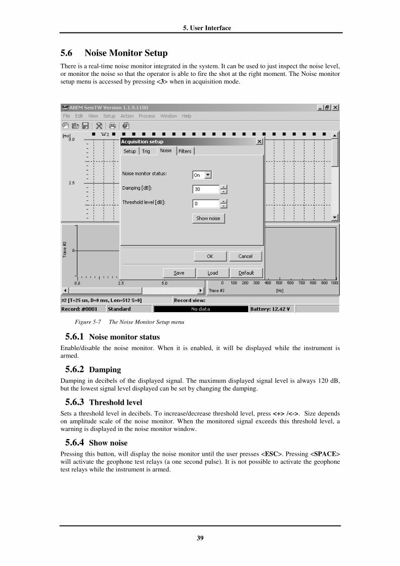
5. User Interface

39

5.6 Noise Monitor Setup

There is a real-time noise monitor integrated in the system. It can be used to just inspect the noise level, or monitor the noise so that the operator is able to fire the shot at the right moment. The Noise monitor setup menu is accessed by pressing <3> when in acquisition mode.

Figure 5-7 The Noise Monitor Setup menu

5.6.1 Noise monitor status

Enable/disable the noise monitor. When it is enabled, it will be displayed while the instrument is armed.

5.6.2 Damping

Damping in decibels of the displayed signal. The maximum displayed signal level is always 120 dB, but the lowest signal level displayed can be set by changing the damping.

5.6.3 Threshold level

Sets a threshold level in decibels. To increase/decrease threshold level, press <+> /<->. Size depends on amplitude scale of the noise monitor. When the monitored signal exceeds this threshold level, a warning is displayed in the noise monitor window.

5.6.4 Show noise

Pressing this button, will display the noise monitor until the user presses <ESC>. Pressing <SPACE> will activate the geophone test relays (a one second pulse). It is not possible to activate the geophone test relays while the instrument is armed.

5. User Interface

40

5.7 Geophone Test

This geophone test is more extensive than the geophone check available in the noise monitor. It can be found in the “Action menu” or activated by pressing <SHIFT>+<ARM> when in acquisition mode. This test, records the response from the geophones to an impulse signal. A DC-current is sent to the geophones dislocating the seismic mass of the geophone. When the DC-current is switched off, the mass performs a damped oscillation with its resonance frequency while it comes to rest. Thus, you will get a report on the maximum amplitude of the response, resonance frequency and damping.

The recording of the response starts just before the DC-current is switched off. The response is recorded and an analysis of the recorded test data is made by SeisTW which determines the status of each channel.

After the analysis of the data has been performed, a report will be generated and stored in the working directory on the disk, results are displayed and saved both as a log file and as a record in SG2 format. The current record number is used to create the filename. The filename pattern is: TEST_XXXX.SG2 .

5.8 Acquisition Filter Setup

The Acquisition Filter Setup menu is accessed by pressing <4> when in acquisition mode.

Figure 5-8 The Acquisition Filter Setup Menu

5.8.1 Notch filter

Status

Enables/disables the notch filter. The notch filter is calibrated at factory for either 50 or 60 Hz. The calibrated value is stored in the Windows Registry. Use this when working in vicinity of power lines, otherwise leave it off. A spectrum analysis of a noise recording may often show if power line noise is present.

5.8.2 Analog low-cut filter

Signals usually contain noise from sources such as wind and traffic. This noise often has low frequency. Analog filter removes these frequencies from the signals. However, the filter may also

5. User Interface

41

deteriorate original signals. The higher the cut-off frequency and filter damping, the worse possible distortions become. Using an analog filter is always a compromise.

If the noise level is high, record it. Use the frequency view to analyze it, and to see the actual noise frequency. Thereafter select and use an appropriate analog filter.

If the noise level is not high, do not use the analog filters.

Analog filters affect all channels. Note that you will not be able to recover any incoming signals that are filtered out. Use analog filters only to remove low frequency ground roll. Generally, be cautious about using these filters as there is always a risk that they may eliminate valuable signal information.

Status

Enables/disables the analog low-cut filter.

Slope

Select the slope of the filter. Possible choices are 12 dB/octave and 24 dB/octave.

Cutoff freq.

Selects the low cutoff (3 dB rejection) frequency in Hz. The possible frequency choice depends on the selected slope. You have 16 different cut-off frequencies for each filter slope to choose from, see table 5-2 below.

When choosing filter slope, remember that generally 24 dB/octave filters distort more than 12 dB/octave, but will also damp noise more effectively. Use as low a cut-off frequency as possible - generally twice the maximum noise frequency. A good rule is to start with the 12 dB/octave filter. If the recorded signal is acceptable then keep the filter, otherwise try again with the 24 dB/octave filter.

Table 5-2 Available 3 dB cutoff frequencies (in Hz)

12 dB/octave 24 dB/octave

12 15

24 30

36 45

48 60

60 75

72 90

84 105

96 120

108 135

120 150

132 165

144 180

156 195

168 210

180 225

192 240

5. User Interface

42

5.9 Receiver Spread Dialog

The Receiver Spread Dialog menu is accessed by pressing <5> when in acquisition mode, note that there is a possibility to return to the default settings by using the default button in the receiver spread dialog.

Figure 5-9 Receiver Spread Dialog Menu

5.9.1 Channel

Specifies the channel mapped to each trace. It is possible to map any channel to any trace, and one channel can be mapped to any number of traces. If the reference channel is enabled, it will be mapped to the trace as specified by the corresponding channel.

Enter the channel number using the numeric keys.

Table 5-3 Key commands - Channel mapping

5.9.2 Polarity

Specifies the polarity of the recorded signal. If the polarity is positive, the signal will be stored as it is recorded. If the polarity is negative, the signal will be inverted before it is stored.

5. User Interface

43

Table 5-4 Key commands - Polarity

5.9.3 Stack on

Enables/disables stacking for the specified trace. If the stack for a trace is disabled, data cannot be added (or subtracted) from that stack.

Table 5-5 Key commands - Stack on

5.9.4 Trace on

Enables/disables viewing of the specified trace.

Table 5-6 Key commands - Trace on

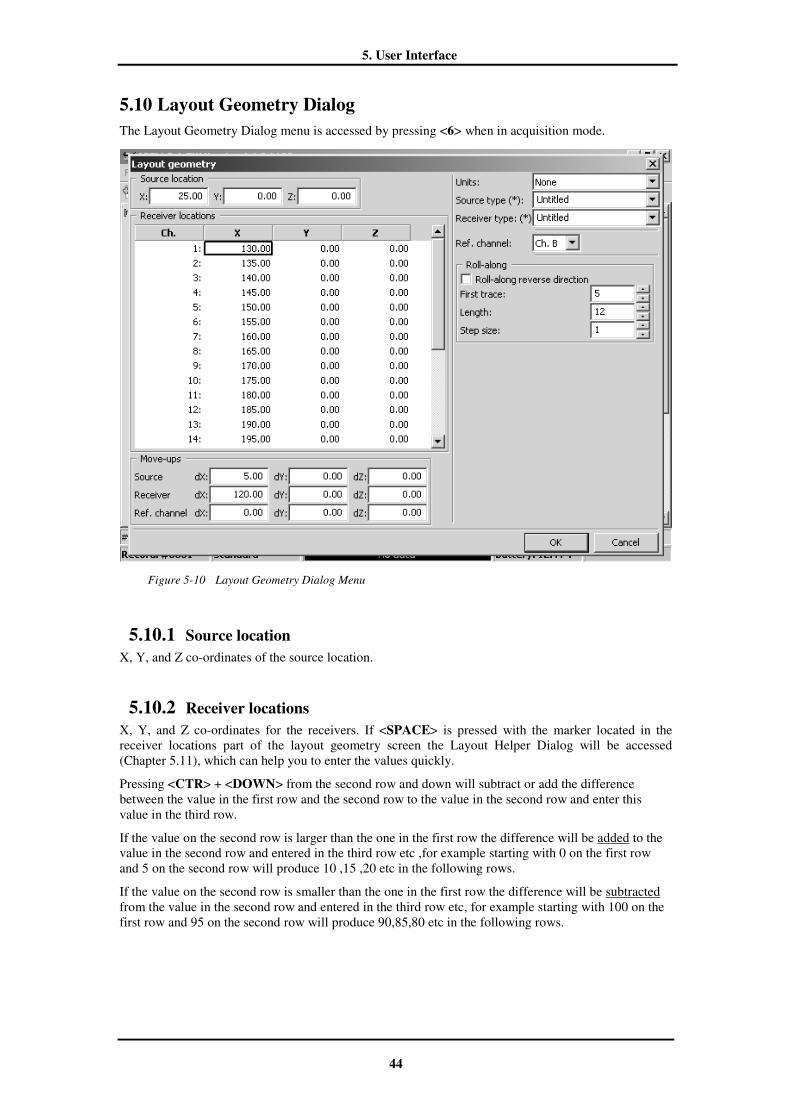
5. User Interface

44

5.10 Layout Geometry Dialog

The Layout Geometry Dialog menu is accessed by pressing <6> when in acquisition mode.

Figure 5-10 Layout Geometry Dialog Menu

5.10.1 Source location

X, Y, and Z co-ordinates of the source location.

5.10.2 Receiver locations

X, Y, and Z co-ordinates for the receivers. If <SPACE> is pressed with the marker located in the receiver locations part of the layout geometry screen the Layout Helper Dialog will be accessed (Chapter 5.11), which can help you to enter the values quickly.

Pressing <CTR> + <DOWN> from the second row and down will subtract or add the difference between the value in the first row and the second row to the value in the second row and enter this value in the third row.

If the value on the second row is larger than the one in the first row the difference will be added to the value in the second row and entered in the third row etc ,for example starting with 0 on the first row and 5 on the second row will produce 10 ,15 ,20 etc in the following rows.

If the value on the second row is smaller than the one in the first row the difference will be subtracted from the value in the second row and entered in the third row etc, for example starting with 100 on the first row and 95 on the second row will produce 90,85,80 etc in the following rows.

5. User Interface

45

5.10.3 Move-ups

Describes how the source, receivers and the receiver connected to the reference channel (if any) are updated when a record has been finished.

Units

Defines the linear units used for all location data. Possible values are: None, Meters, Centimetres, Feet

and Inches. If None is specified it will be up to the user to interpret location data.

Source type (*)

An appropriate text string describing the source used to acquire this record. Pre-defined values are:

Untitled, Hammer, Weight_Drop, Seismic_Gun, Explosives, and Vibrator. The asterisk specifies that the user may enter any text string in this field.

Receiver type (*)

An appropriate text string describing the receivers used to acquire this record. Pre-defined values are: Untitled, Vertical_Geophone, SH_Horizontal_Geophone, SV_Horizontal_Geophone, and Accelerometer. The asterisk specifies that the user may enter any text string in this field.

Ref. channel

Selects if the reference channel connector is activated, and which channel that will be redirected to this connector. It is possible to re-direct either channel 12 or channel 24 to the reference channel connector, the selections are called Ch. A and Ch. B. With more than 24 channels installed (i.e. typically 48 channels), it is channels 24 or channel 48 that can be redirected to this connector.

5.10.4 Roll-along

The settings used to control roll-along measurements (see Mode: Roll along). Note that it is assumed that the lowest numbered trace on the left side and the highest numbered on the right side.

If needed, the channels can be re-mapped as in any other acquisition mode.

Roll-along reverse direction

If checked, the roll-along segments will be shifted to the left (normally they are shifted to the right).

First trace

The first (left most) trace of the current cable layout for the current record.

Length

Number of traces comprising one roll-along segment.

Step size

Number of steps to shift the roll-along after finishing a record.

5. User Interface

46

5.11 Layout Helper

The Layout Helper menu is accessed by pressing <SPACE> when in Receiver locations part of the Layout Geometry Dialog menu.

Figure 5-11 The Layout Helper menu

The Layout helper dialog can be used to quickly fill in the receiver locations in the Layout geometry dialog. It is possible to enter values in any two of the entries layout start, layout end, and receiver separation. The third entry is calculated automatically.

Pressing <SPACE> in a cell belonging to one of the above entries, causes this entry to become the one that is calculated automatically. Selecting OK to exit from the dialog, causes the receiver locations grid to be filled out automatically.

5.11.1 Layout start

X, Y, and Z co-ordinates of the first receiver of the layout.

5.11.2 Layout end

X, Y, and Z co-ordinates of the last receiver of the layout.

5.11.3 Receiver separation

The receiver separation in x-, y-, and z-directions, respectively.

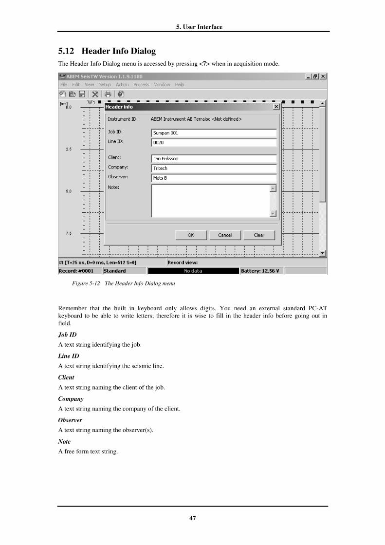
5. User Interface

47

5.12 Header Info Dialog

The Header Info Dialog menu is accessed by pressing <7> when in acquisition mode.

Figure 5-12 The Header Info Dialog menu

Remember that the built in keyboard only allows digits. You need an external standard PC-AT keyboard to be able to write letters; therefore it is wise to fill in the header info before going out in field.

Job ID

A text string identifying the job.

Line ID

A text string identifying the seismic line.

Client

A text string naming the client of the job.

Company

A text string naming the company of the client.

Observer

A text string naming the observer(s).

Note

A free form text string.

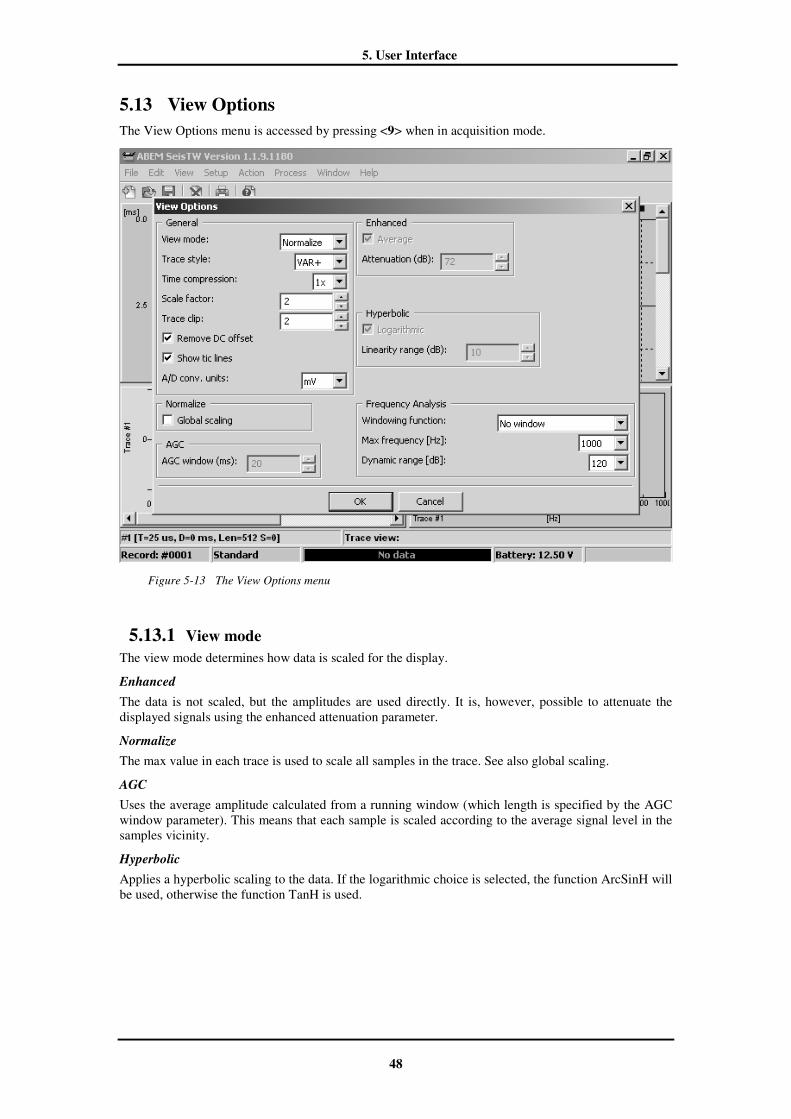
5. User Interface

48

5.13 View Options

The View Options menu is accessed by pressing <9> when in acquisition mode.

Figure 5-13 The View Options menu

5.13.1 View mode

The view mode determines how data is scaled for the display.

Enhanced

The data is not scaled, but the amplitudes are used directly. It is, however, possible to attenuate the displayed signals using the enhanced attenuation parameter.

Normalize

The max value in each trace is used to scale all samples in the trace. See also global scaling.

AGC

Uses the average amplitude calculated from a running window (which length is specified by the AGC window parameter). This means that each sample is scaled according to the average signal level in the samples vicinity.

Hyperbolic

Applies a hyperbolic scaling to the data. If the logarithmic choice is selected, the function ArcSinH will be used, otherwise the function TanH is used.

5. User Interface

49

5.13.2 Trace style

VAR+

This is a wiggle trace with the positive side filled-in.

VAR-

This is a wiggle trace with the negative side filled-in.

Wiggle

The trace is plotted as a wiggle.

Dotted

Each sample value is plotted as a dot.

5.13.3 Time compression

Selects compression in time. This makes more of the record visible. Available compressions: 1x, 2x, 4x,

and 8x.

5.13.4 Scale factor

A general factor by which every sample is multiplied.

5.13.5 Trace clip

How many traces the plotted curve may overlap before it is clipped. With trace clip = 1, no overlap will occur. If trace clip is 2, a trace may overlap the positive part of the trace on the left, and the negative part of the trace on the right.

5.13.6 Remove DC offset

If enabled, the DC offset is removed before the trace is scaled. It is recommended to keep this enabled.

5.13.7 Show tic lines

Major and minor tic lines are plotted. The time interval between the tic lines is determined by sample interval and time compression.

5.13.8 Normalize

Global scaling

If enabled, the maximum value in the whole record is used to normalize every sample of all traces.

5.13.9 AGC

AGC window

The length of the window, in milliseconds, used to calculate the average value to use for scaling of a sample value. The window moves along the trace with each sample that is scaled.

5. User Interface

50

5.13.10 Enhanced

Average

If enabled, the average values on the stack is used for each trace, otherwise the summed stack is used.

Attenuation

Used to attenuate the signals. This will bring out weaker signals, while hiding stronger signals.

5.13.11 Hyperbolic

Logarithmic

If enabled, ArcSinH is used a scaling function, otherwise, TanH is used.

Linear range

This value sets the amplitude level that is within the linear part of the scaling function. Both scaling functions are linear in the beginning (for small amplitudes), while compressing larger amplitudes.

5.13.12 Frequency analysis

Windowing function

Selects function to be used for data windowing. Possible values are No window, Hanning,

Hamming, Blackman, Bartlett, Kaiser, 4th order Blackman-Harris, Flat top.

Max frequency

The maximum frequency to display. The displayed spectrum will go from 0 Hz up to the selected maximum frequency. Possible values are 50, 100, 200, 500, 1000, 2000, 5000, 10000, 20000, 50000.

Dynamic range

The maximum frequency component is used as reference when calculating the spectrum. The dynamic range can be set to 6 dB up to 198 dB in 6 dB steps.

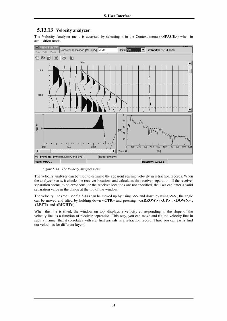
5. User Interface

51

5.13.13 Velocity analyzer

The Velocity Analyzer menu is accessed by selecting it in the Context menu (<SPACE>) when in acquisition mode.

Figure 5-14 The Velocity Analyzer menu

The velocity analyzer can be used to estimate the apparent seismic velocity in refraction records. When the analyzer starts, it checks the receiver locations and calculates the receiver separation. If the receiver separation seems to be erroneous, or the receiver locations are not specified, the user can enter a valid separation value in the dialog at the top of the window.

The velocity line (red , see fig 5-14) can be moved up by using <-> and down by using <+> , the angle can be moved and tilted by holding down <CTR> and pressing <ARROW> (<UP> , <DOWN> , <LEFT> and <RIGHT>).

When the line is tilted, the window on top, displays a velocity corresponding to the slope of the velocity line as a function of receiver separation. This way, you can move and tilt the velocity line in such a manner that it correlates with e.g. first arrivals in a refraction record. Thus, you can easily find out velocities for different layers.

5. User Interface

52

5.14 Optimizing

Many of the settings you select affect the performance of the system. You can set up the system to do the data acquisition as fast as possible, or to give you as much information during the acquisition as possible (often this means a more secure operation).

5.14.1 Optimize For Speed

Sometimes, for example in marine seismic surveys, it is important to obtain fast data acquisition. There are some operations that can be modified, or even skipped, to enhance the acquisition speed. Still, there are some operations that are fixed, and to this category belong the actual data acquisition (sampling procedure), transfer of the data from acquisition memory to trace memory, and writing of the data to disk.

However, the following should be considered:

• Do not display data after shooting, i.e. use "Fast stack", since scaling of traces takes a considerable time.

• Use as short records as possible (number of samples).

5.14.2 Optimize For Security

When you optimize for security, you set the instrument up, to give you as much information about the data acquisition as possible. This means that, e.g. data and progress are displayed.

• Use "Preview" or "Single" stack modes.

• Use the noise monitor if you are in Stack Once mode.

5.15 Data Safety

It is highly advisable to make backup copies of recorded data , as with every computerized system there is always a slight risk that data could be lost due to hardware failure or corrupted data, ABEM can not take responsibility for recorded data that is lost.

6. Process

53

6. PROCESS

6.1 First breaks

These entries are accessed via a sub menu in the Context menu (<SPACE>)

6.1.1 Auto

Performs an automatic first break pick. Automatic computing of first arrivals works best on data with small pre-signal noise. You should always check the picked arrivals and edit any bad picks. If there is one or more picks for this record, you will be warned before times are picked automatically.

6.1.2 Clear

Clears the first break picks.

6.1.3 Save

Saves the first break picks to a text file in the current directory. There are two formats available, ABEM's fir-format, and REFLEXW's pck-format. Choose format when saving the first break picks (fig 6-1 ).

Figure 6-1 First breaks menu with the Save first arrival times dialog

6.1.4 Load

Loads the first break picks from a pick file to the currently active record. If there are more picks in the pick file than traces in the record, the superfluous picks are discarded. If there are fewer picks, only the first traces loads the picks.

6. Process

54

6.2 FIR Filter

The FIR filter menu is accessed by selecting it in the Context menu (<SPACE>). About the first arrival file format see chapter 9.5 (APPENDIX A).

Figure 6-2 FIR Filter menu

Clicking OK will apply the filter to the current data.

6.2.1 Filter type

Selects the type of filter to apply to data. Available choices are Low pass, high pass, band pass, and band reject.

Low pass

Rejects frequencies higher than the high cut-off.

High pass

Rejects frequencies lower than the low cutoff.

Band pass

Rejects frequencies lower than the low cut-off and higher than the high cut-off.

Band reject

Rejects frequencies between the low cut-off and high cut-off.

6.2.2 Windowing function

Data windowing function to apply to data when filtering. Available choices are Hanning and Blackman.

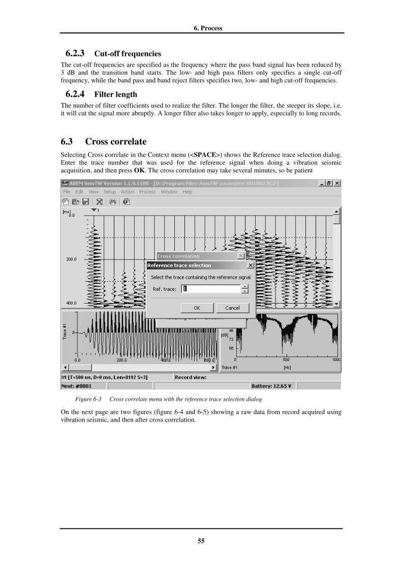
6. Process

55

6.2.3 Cut-off frequencies

The cut-off frequencies are specified as the frequency where the pass band signal has been reduced by 3 dB and the transition band starts. The low- and high pass filters only specifies a single cut-off frequency, while the band pass and band reject filters specifies two, low- and high cut-off frequencies.

6.2.4 Filter length

The number of filter coefficients used to realize the filter. The longer the filter, the steeper its slope, i.e. it will cut the signal more abruptly. A longer filter also takes longer to apply, especially to long records.

6.3 Cross correlate

Selecting Cross correlate in the Context menu (<SPACE>) shows the Reference trace selection dialog. Enter the trace number that was used for the reference signal when doing a vibration seismic acquisition, and then press OK. The cross correlation may take several minutes, so be patient

Figure 6-3 Cross correlate menu with the reference trace selection dialog

On the next page are two figures (figure 6-4 and 6-5) showing a raw data from record acquired using vibration seismic, and then after cross correlation.

6. Process

56

Figure 6-4 Raw data

Figure 6-5 After cross correlation

6. Process

57

6.4 Moving average

Selecting Moving Average in the context menu (<SPACE>), shows the Enter filter length dialog.

Figure 6-6 The Moving Average menu

Perform a moving average filtering of the current data . The user selects the number of samples to use when calculating the average.

7. Triggering Methods

59

7. TRIGGERING METHODS To make a recording with the TERRALOC seismic system, an initiating trigger signal is required. The trigger pulse defines the start of the data recording and is the reference for all timing.

7.1 Make/Break Switch Input

The system will trigger if the wires of the trigger cable are shorted together (make switch), or if the shorted wires are opened (break switch).

When you use explosives, one trigger method is to put a few turns of wire around the charge. The wire is cut by the explosion and triggers the seismograph (break switch). You can also twist a pair of insulated wires together and insert the twisted part into the dynamite. The explosion will compress the wires and crush/melt the insulation causing the leads of the wires to short together. This will trigger the seismograph (make switch).

Besides, this make switch triggering method can be applied when you use falling weight or hammer as energy source. However, you must use a metallic shock plate and the falling weight or the hammer head must be made out of metal. Connect one lead of the trigger wire to the shock plate and the other lead to the falling weight or hammer head. When the hammer hits the shock plate, the trigger circuit is shorted and the instrument triggers.

7.2 Using The Trigger Coil

If you want to trigger TERRALOC Mk6 / Mk8 with the ignition current going out to the charge, you can use the Trigger Coil (current detector unit) included in the TERRALOC Mk6 / Mk8 accessories. To use this you merely feed one of the two shot wires through the hole in the trigger coil. The trigger coil is either connected directly to the trigger input or to the extension connectors on the trigger cable reel. Then set the TERRALOC in the "Analog" trigger input mode with the sensitivity control set at about 50 %. When the charge is fired, the ignition current will trigger TERRALOC instantly. The current pickup trigger method is very convenient since you only need to bring the shot cable to the shot hole.

NOTE! You have to use (seismic) blasting caps with no built-in delay to be able to use this method. If you use ordinary blasting caps the ignition delay will be included in your record. There are seismic blasting caps of the safety type available. Their delay is only some 50 µs if fired with a high power blasting machine.

7.3 Radio Triggering

In case you need to trigger the TERRALOC in places where you cannot use a trigger cable, you can use a simple radio equipment to transmit the trigger pulse.

8. Troubleshooting

61

8. TROUBLESHOOTING Although great care has been taken to make TERRALOC Mk6 / Mk8 as reliable as possible, it is always a small risk that something does not work properly. Should you have trouble getting things to work, please refer to chapter 8. This is a guide to the common problems and how to work them out.

8.1 General SeisTw Program Problems

These errors are generally related to the software.

8.1.1 The Program Does Not Start

There should normally be no problem starting SeisTW in the TERRALOC Mk6 v2 / Mk8 once it has been installed and runs. However, if SeisTW doesn’t start when starting the instrument for some reason you may need to reinstall. Follow install instructions in Chapter 9 (APPENDIX A ).

8.2 Data Acquisition Problems

The data acquisition problems can range from errors in the setting up of the system for measurement, over hardware problems, to errors in the settings in the software.

8.2.1 TERRALOC Only Waits For Confirmation When Arming

If the instrument shows the status message "<<<Pending ARM ...>>>" when you try to arm the instrument, it means that External Arm input mode is set to TTL Rising edge or TTL Falling edge. If it is, it will wait for an external arm signal to arrive before it arms itself. This is used when you interconnect two or more TERRALOC´s.

If you use one TERRALOC only, no external arm will arrive, hence the TERRALOC never arms (unless you have some other external device that confirms the arm command). Set External Arm input to Off and the arming will be normal.

8.2.2 Dead Channels

Check the Receiver Spread Menu for the settings of the "Stack On" and "Trace On" parameters. You should also check the reference channel setting in the Receiver Layout Menu.

8.2.3 Data Is Not Displayed

Check if you have selected Fast Stack as stacking mode, as this causes data not to be displayed on the screen. In case of, Auto Stack, Preview and Single, check that the "Trace" parameters in the Receiver Spread Menu are activated.

8.2.4 Large Offset

Check offset level and do not worry if it is less than 2000 units.

8.2.5 Incorrect Channel Order

Either one cable - at least - has been reversed in the layout or the channel assignments are erroneous. Check the cable and/or the channel assignments in the Receiver Spread Menu. Please be aware that a reversed cable can be corrected for in the Receiver Spread Menu.

8. Troubleshooting

62

8.3 Trigger Problems

Correct triggering is essential for the quality of the data from the acquisition, especially when it comes to timing. This means that you should be very careful when selecting triggering method and setting up the triggering system. It may not always be obvious that there is something wrong with the trigger.

8.3.1 Triggering Too Late (Or Early)

This is usually caused by erroneous setting of the trigger sensitivity when analog triggering is used. Adjust the sensitivity level so the trigger pulse is detected correctly (see also chapter 5.5.2 ).

8.3.2 Spurious Triggering

This is usually caused by too high trigger sensitivity, resulting in triggering on pretrig event noise. Adjust the sensitivity level so the trigger pulse is detected correctly (see also chapter 5.5.2 ).

If you are using radio triggering, check also the signal levels of the transmitter and receiver respectively.

8.3.3 Unable To Trigger

The trigger sensitivity might have been set too low, or the type of trigger input does not agree with the trigger method used. Check the trigger settings and the trigger cable, there may be a break in the cable or a bad connection somewhere.

Select "Make/Break" trig input mode (the trigger input level should be about 50%) and try to short trigger input by a bare wire. The instrument should trigger when you make or when you break connection. If the instrument does not trigger, then you might have a fault in the internal triggering electronics.

8.3.4 Triggering Immediately When Arming

If you are using analog triggering, the trig sensitivity might have been set too high. At the highest sensitivity level, even internal electronic circuitry noise may cause triggering.

When digital triggering is used (i.e. TTL Rising edge or TTL Falling edge), you must have the correct setting (rising or falling) according to the trigger signal received. For example, if the trig event is indicated by a logical 1, the trigger input type should be set to "TTL Rising edge". In this case, the idle trigger signal must be a "0" , otherwise the instrument will be triggered continuously.

9. Appendix A

63

9. APPENDIX A

9.1 Software Installation

TERRALOC Mk6 / Mk8 is delivered with all necessary software installed at the factory. However, if the software needs to be updated, or re-installed, the procedure is described below. When the installation has finished, verify that the SeisTW version is correct, and that the device driver and API version are identical. This information can be found in the About dialog (press <CTR>+<HLP>).

9.2 Install procedure for SeisTW

Copy the setup file “SetupSeisTW.exe” to the hard drive of the TERRALOC Mk6 / Mk8 and double-click to start the setup, follow the instructions in the setup wizard and verify that all three boxes are

checked to install TERRALOC drivers, SeisTW and examples, see picture below.

Figure 9-1 SeisTW Setup - Select Components

Then click on the next button, submit the serial number of the instrument and verify that the number of channels corresponds to the number of channels installed in the instrument, also verify that the notch filter frequency is set to the correct value, usually 50Hz unless the instrument has been specifically ordered with 60Hz notch filter, see figure 9-2 on the next page.

9. Appendix A

64

Figure 9-2 SeisTW Setup – Terraloc Configuration

After this is done click on the “Install button”, setup will now install all necessary files for SeisTW.

When it says “completed” at the bottom of the setup window click “Next” and then “Finish”, you will then be asked if you want to reboot the system, to be able to start using SeisTW you will need to reboot.

TERRALOC Mk6 / Mk8 will now restart and automatically launch SeisTW.

9.3 Boot preparations

TERRALOC Mk6 v2 wasn’t delivered with SeisTW installed from the factory since SeisTW wasn’t available, therefore it needs to be installed and also some changes needs to be made to get the TERRALOC to boot to Windows XP and SeisTW by default.

The boot.ini file needs to be changed from the default (seen below fig 9-3 ), the line “default=C:\“ needs to be changed to the yellow marked text seen in fig 9-4 , otherwise the TERRALOC will not boot to Windows/SeisTW by default (since the red marked text is identical you may use it to copy/paste)

The green marked text is however optional ,to better indicate which boot choices there are you might want to change the green marked text line to “SeisTW (Windows XP)” for example.

The boot.ini settings can be accessed and changed in the controlpanel in Windows under “Performance and Maintenance-System-Advanced-Startup and Recovery-Settings-Edit”

WARNING ! :Be careful editing these boot settings, if incorrect settings is applied computer may not boot, the boot.ini file can also be edited using a DOS boot diskette containing the program “Edit” if boot problems should occur.

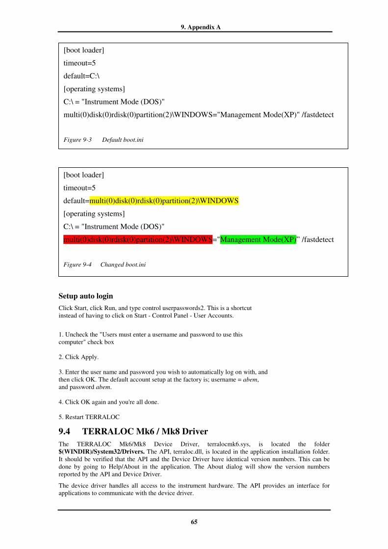
9. Appendix A

65

Setup auto login

Click Start, click Run, and type control userpasswords2. This is a shortcut instead of having to click on Start - Control Panel - User Accounts.

1. Uncheck the "Users must enter a username and password to use this computer" check box 2. Click Apply. 3. Enter the user name and password you wish to automatically log on with, and then click OK. The default account setup at the factory is; username = abem, and password abem. 4. Click OK again and you're all done. 5. Restart TERRALOC

9.4 TERRALOC Mk6 / Mk8 Driver

The TERRALOC Mk6/Mk8 Device Driver, terralocmk6.sys, is located the folder $(WINDIR)/System32/Drivers. The API, terraloc.dll, is located in the application installation folder. It should be verified that the API and the Device Driver have identical version numbers. This can be done by going to Help/About in the application. The About dialog will show the version numbers reported by the API and Device Driver.

The device driver handles all access to the instrument hardware. The API provides an interface for applications to communicate with the device driver.

[boot loader]

timeout=5

default=multi(0)disk(0)rdisk(0)partition(2)\WINDOWS

[operating systems]

C:\ = "Instrument Mode (DOS)"

multi(0)disk(0)rdisk(0)partition(2)\WINDOWS="Management Mode(XP)” /fastdetect

Figure 9-4 Changed boot.ini

[boot loader]

timeout=5

default=C:\

[operating systems]

C:\ = "Instrument Mode (DOS)"

multi(0)disk(0)rdisk(0)partition(2)\WINDOWS="Management Mode(XP)" /fastdetect

Figure 9-3 Default boot.ini

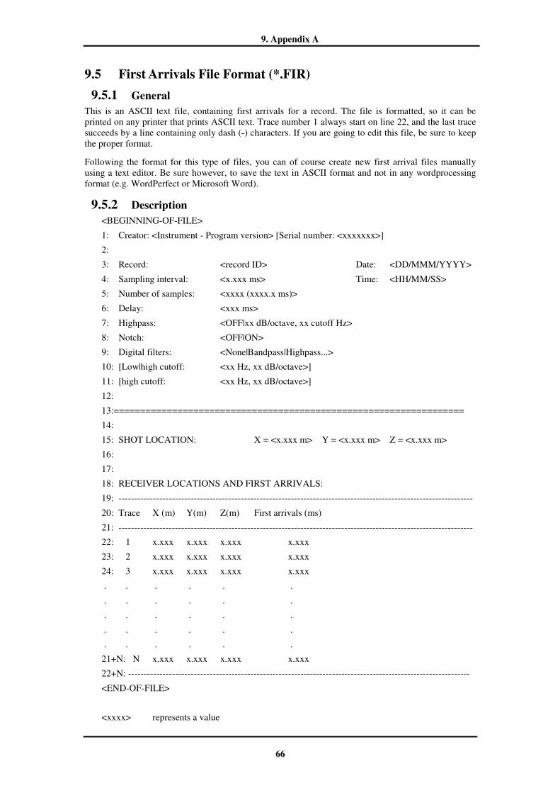
9. Appendix A

66

9.5 First Arrivals File Format (*.FIR)

9.5.1 General

This is an ASCII text file, containing first arrivals for a record. The file is formatted, so it can be printed on any printer that prints ASCII text. Trace number 1 always start on line 22, and the last trace succeeds by a line containing only dash (-) characters. If you are going to edit this file, be sure to keep the proper format.

Following the format for this type of files, you can of course create new first arrival files manually using a text editor. Be sure however, to save the text in ASCII format and not in any wordprocessing format (e.g. WordPerfect or Microsoft Word).

9.5.2 Description

<BEGINNING-OF-FILE>

1: Creator: <Instrument - Program version> [Serial number: <xxxxxxx>]

2:

3: Record: <record ID> Date: <DD/MMM/YYYY>

4: Sampling interval: <x.xxx ms> Time: <HH/MM/SS>

5: Number of samples: <xxxx (xxxx.x ms)>

6: Delay: <xxx ms>

7: Highpass: <OFF|xx dB/octave, xx cutoff Hz>

8: Notch: <OFF|ON>

9: Digital filters: <None|Bandpass|Highpass...>

10: [Low|high cutoff: <xx Hz, xx dB/octave>]

11: [high cutoff: <xx Hz, xx dB/octave>]

12:

13:==================================================================

14:

15: SHOT LOCATION: X = <x.xxx m> Y = <x.xxx m> Z = <x.xxx m>

16:

17:

18: RECEIVER LOCATIONS AND FIRST ARRIVALS:

19: -----------------------------------------------------------------------------------------------------------------

20: Trace X (m) Y(m) Z(m) First arrivals (ms)

21: -----------------------------------------------------------------------------------------------------------------

22: 1 x.xxx x.xxx x.xxx x.xxx



. . . . . .

. . . . . .

. . . . . .

. . . . . .

. . . . . .

21+N: N x.xxx x.xxx x.xxx x.xxx

22+N: -------------------------------------------------------------------------------------------------------------

<END-OF-FILE>

<xxxx> represents a value

9. Appendix A

67

[xxxx] denotes optional text

| delimits possible values

10. Appendix B

69

10. APPENDIX B

10.1 Connectors

10.1.1 Seismic Input Connectors

Seismic Input connector 24 channel TERRALOC Mk6 / Mk8

Connector type:

Cannon NK-27-32P Panel connector (mating side) (fits to NK-27-21C-1/2 ” cable connector)

Figure 10-1 Seismic input connector 24 channel TERRALOC

Connector 1-12 Connector 13-24

Pin Channel Pin Channel

1 1+ 1 13+

2 1- 2 13-

3 2+ 3 14+

4 2- 4 14-

“ “ “ “

“ “ “ “

23 12+ 23 24+

24 12- 24 24-

10. Appendix B

70

Seismic Input connector 48 channel TERRALOC Mk6 / Mk8

Connector type:

Cannon KPT-02-A22-55P Panel connector (mating side) (fits to KPT-06 A22-55S cable connector)

Figure 10-2 Seismic input connector 48 channel TERRALOC

Connector 1-24 Connector 25-48

Pin Channel Pin Channel

A 24+ A 25+

B 24- B 25-

C 23+ C 26+

D 23- D 26-

“ “ “ “

“ “ “ “

Z 13+ Z 36+

a 13- a 36-

b 12+ b 37+

c 12- c 37-

“ “ “ “

“ “ “ “

z 1+ z 48+

AA 1- AA 48-

10. Appendix B

71

10.1.2 Power Connector

Connector type: Cannon AXR-3-32 (mating side), (fits to AXR-3-11 cable connector.)

(Mating side view)

Figure 10-3 Power connector

1 Negative power supply (-)

2 Positive power supply (+)

3 Positive power supply (+)

10.1.3 TTL Arm/Trig Connector

Connector type: KPT 02-E10-6P (fits to KPT 06-E10-6S cable connector.)

(Mating side view)

Figure 10-4 TTL Arm/Trig connector

A Trigger Output B Arm Input C Trigger Input D GND (Ground) E No Connection F Arm Output

11. Appendix C

73

11. APPENDIX C

11.1 SEISMIC methods

There is a variety of seismic methods used. The objective of the survey controls which specific method to use. This section will give you an overview of some commonly used methods. Please refer to the bibliography at the end of the manual, if you need a more detailed and thorough description of seismic methods, where Butler (2005) can be recommended as it is new and has an extensive and recently updated listing of references

In the refraction and reflection methods, there is usually a division between shallow and deep surveys.

11.1.1 Refraction

The objective is to find out the arrival times of the head waves to map the depth to the refractors in which the waves travel. The refraction method is based on the assumption that the earth is made of layers of materials that increase in seismic velocity with each successively deeper layer. The key element is that an incident ray is critically refracted along the boundaries between layers, before returning to the surface. From the first arrival times it is possible to calculate the seismic velocity for each layer and the depth to the boundaries. The seismic velocity gives information about material properties, and what kind of material comprises each layer. Additionally, frequency analysis of the recorded signals can give more information about the material properties.

The principles for seismic refraction techniques can be found in most geophysical textbooks. For a more detailed description of both theory and practice, see Sjögren (1984).

Investigations performed with the refraction method, can yield a variety of reliable data such as depth of various overburden layers, depth to bedrock, soil compositions and solidity, rock quality, rippability, excavability, water tables and rock structure.

The refraction seismic method can be used for a wide range of applications, for example:

Underground Tunnels and their entrances, machinery halls, gas and oil storage facilities, air raid shelters.

Foundations Heavy industrial buildings, bridges, harbour quays and breakwaters, dams, piling, airfields.

Excavations Harbour basins and entrances, pipelines, canals, roads, railways.

Resource searches Gravel, sand and quarry sites.

Water prospecting Groundwater table in the overburden, water bearing sections of rock.

Ore prospecting Mineralized weathered zones, buried channels with high mineral content.

11.1.2 Reflection

In this method, the arrival time events are attributed to seismic waves that have been reflected from interfaces where changes in acoustic impedance occur, and of wave shape changes.

The seismic reflection method has mainly been used for deep investigations (depth > 30 m) in oil prospecting. During recent years however, shallow reflection investigations have become common for engineering and environmental purposes. It is now an important complement to refraction investigations, and has even sometimes replaced refraction. The main reasons for the increase in use of the reflection method is the development of light weight, high-performance seismographs and the possibility of advanced data processing on inexpensive personal computers. Thus, the cost for reflection investigations has decreased considerably.

Both acquisition and processing of reflection data are more complex and time consuming than they are for refraction data.

11. Appendix C

74

11.1.3 Optimum Offset

This is a special case of the seismic reflection method, in which data are recorded with a fixed source-receiver offset. It is a method for shallow investigations. The offset is chosen to be an optimum value (hence the name), and typically, it is a window where the reflection from the target is located between the refracted first arrivals and the ground roll in the seismogram.

11.1.4 Tomography

The general idea for tomography is that information about the properties of the interior of a region can be obtained through measurements at the boundary. Thus, this is a method for finding the (2-dimensional) distribution of some physical property (e.g. velocity, reflectivity, bulk modulus, etc.). It can involve borehole-to-borehole, surface-to-borehole, or surface-to-surface measurements. The main restriction is that the source and receiver positions, and hence any boreholes, must be confined to the same plane. This plane can have any orientation.

Usually, the travel times for a large number of ray paths through the rock volume are measured, and sometimes, even amplitudes (direct or reflected) are analyzed. Then the dataset goes through an inversion process, where the spatial distribution of the physical property is estimated. The technique is very computational intensive, and is costly because of the need for boreholes.

The final results are usually presented as maps or plots, where the values of the physical property are coded in color or grayscale.

An introduction to this method can be found in Worthington (1984).

11.1.5 VSP

VSP is short for Vertical Seismic Profiling, i.e. measurements with the receivers located in a borehole and the source located on the ground. If the source is moved away from the head of the borehole, it is called "offset VSP". In "Reversed VSP", the receivers are located on the ground and the source is located in the borehole.

The VSP technique is seldom used alone, but is rather used to provide better interpretation of seismic reflection data. VSP allows accurate determination of one-way travel time to various geologic units and analysis of attenuation and acoustic impedances which are needed for construction of synthetic seismograms.

A brief introduction to this method is given in Cassel (1984).

11.1.6 Vibroseis

Vibroseis is a seismic method in which a vibrator is used as an energy source to generate a controlled wavetrain, instead of the usual impulsive sources (e.g. hammer, explosives, shot guns, etc.). This method requires recording of the source signal for reference.

A sinusoidal vibration of continuously varying frequency is applied during a sweep period typically lasting for several seconds (>10 s.). The sweep may start at either low, or high frequencies, and it can be linear or nonlinear. The recorded data, comprising many superpositioned wavetrains, has to be correlated with the source signal. . The correlated record resembles a conventional seismic record such as results from an impulsive source.

12. Bibliography

75

12. BIBLIOGRAPHY Butler, Dwain K., Editor. 2005. Near Surface Geophysics. Volume 13 in Series: Investigations in

Geophysics. Society of Exploration Geophysicists. ISBN 1-56080-130-1.

Cassel, Bruce. 1984. Vertical Seismic Profiling - an Introduction. First Break Vol. 2 No. 11. European Association of Exploration Geophysicists.

Palmer, Derecke. 1980. The Generalized Reciprocal Method of Seismic Refraction Interpretation. Society of Exploration Geophysicists. ISBN 0-931830-14-1.

Parasnis, D.S. 1986. Principles of Applied Geophysics. 4th Ed. Chapman and Hall. ISBN 0-412-28330-1.

Penoyer, Robert 1993. The Alpha-Beta filter. The C Users Journal Vol. 11 No. 7 (73-86). R&D Publications.

SEG 1990. Seismic (/Radar) Files in Personal Computers Standard. Engineering and Groundwater Geophysics Subcommittee, Society of Exploration Geophysicists. ISBN 1-56080-020-8

Sheriff, Robert E. 1991. Encyclopedic Dictionary of Exploration Geophysics. 3rd Edition. Society of Exploration Geophysicists. ISBN 0-931830-47-8 (Series), ISBN 1-56080-018-6 (Volume).

Sjögren, Bengt. 1984. Shallow Refraction Seismics. Chapman and Hall. ISBN 0-412-24210-9.

Ward, Stanley H., Editor. 1990. Geotechnical And Environmental Geophysics Vol I-III. Volume 5 in Series: Investigations in Geophysics (Edwin B. Neitzel, Series Editor). Society of Exploration Geophysicists. ISBN 0-931830-99-0.

Worthington, M.H. 1984. An Introduction To Geophysical Tomography. First Break Vol. 2 No. 11. European Association of Exploration Geophysicists.

Yilmaz, Özdogan. 1987. Seismic Data Processing. Volume 2 in Series: Investigations in Geophysics (Edwin B. Neitzel, Series Editor). Society of Exploration Geophysicists. ISBN 0-931830-40-0

TERRALOC MK6 v2 och Mk8 Reference manual Windows XP ... · TERRALOC Seismic System Reference Manual...

Documents

Transcript of TERRALOC MK6 v2 och Mk8 Reference manual Windows XP ... · TERRALOC Seismic System Reference Manual...