Terrain Influences on Synoptic Storm Structure and MesoscalePrecipitation Distribution during IPEX IOP3

Jason C. ShaferNOAA Cooperative Institute for Regional Prediction and Department of Meteorology, University

of Utah, Salt Lake City, Utah

W. James SteenburghNOAA Cooperative Institute for Regional Prediction and Department of Meteorology, University

of Utah, Salt Lake City, Utah

Justin A. W. CoxNOAA Cooperative Institute for Regional Prediction and Department of Meteorology, University

of Utah, Salt Lake City, Utah

John P. MonteverdiSan Francisco State University, San Francisco, California

Submitted toMonthly Weather ReviewNovember 22, 2004

––––––––––––––––––––––––––Corresponding author address:Jason C. ShaferUniversity of UtahDepartment of Meteorology135 South 1460 East Room 819Salt Lake City, UT 84112-0110jshafer@met.utah.edu

2

Abstract

The influence of topography on the evolution of a winter storm over the western United

States and distribution of precipitation over northern Utah are examined using data collected

during IOP3 of the Intermountain Precipitation Experiment (IPEX). The analysis is based on

high-density surface observations collected by the MesoWest cooperative networks, special

radiosonde observations, wind profiler observations, NEXRAD radar data, and conventional data.

A complex storm evolution was observed, beginning with frontal distortion and low-level

frontolysis as a surface occluded front approached the Sierra Nevada. As the low-level occluded

front weakened, the associated upper-level trough moved over the Sierra Nevada and overtook a

lee trough. The upper-level trough, which was forward sloping and featured more dramatic

moisture than temperature gradients, then moved across Nevada with a weak surface reflection as

a pressure trough.

Over northern Utah, detailed observations revealed the existence of a midlevel trough

beneath the forward-sloping upper-level trough. This midlevel trough appeared to form along a

high potential vorticity banner that developed over the southern Sierra Nevada and was advected

downstream over northern Utah. A surface pressure trough moved over northern Utah 3 h after the

midlevel trough and delineated two storm periods. Ahead of the surface trough, orographic

precipitation processes dominated and produced enhanced mountain precipitation. This period

also featured lowland precipitation enhancement upstream of the northern Wasatch Mountains

where a windward convergence zone was present. To the south, however, precipitation shadowing

produced by the Oquirrh and Stansbury Mountains lowered precipitation amounts across the Salt

Lake and Tooele Valleys. Precipitation behind the surface trough was initially dominated by

orographic processes, but soon thereafter featured convective precipitation that was not fixed to

the terrain. Processes responsible for the complex vertical trough structure and precipitation

distribution over northern Utah are discussed.

3

1. Introduction

A major winter storm affected much of the western United States on 12–13 February

2000. Across the lowlands of north-central California, heavy rains produced flooding, the collapse

of a Home Depot roof in Colma, and more than 2 million dollars of damage (NCDC 2000, p. 29).

Mountain snows of 60–120 cm (2–4 ft) fell over the Sierra Nevada, and prefrontal wind gusts

reaching 26 m s-1 uprooted trees across parts of southern California (NCDC 2000, p. 26–27).

Over northern Utah, the storm was responsible for 60–90 cm of mountain snow, and up to 2.1 cm

of snow water equivalent (SWE) at lowland locations. Significant precipitation gradients were

observed over northern Utah. For example, the mountain site Snowbasin (SNI, 2256 m) recorded

4.9 cm SWE, over twice the 2.1 cm which fell at Ogden (OGD, 1360m), a lowland site only 15

km away. In addition, significant precipitation contrasts were observed between sites at

comparable elevations. For example, the 2.1 cm of SWE at OGD was nearly four times greater

than the 0.6 cm observed 45 km away at Salt Lake City (SLC, 1280 m). The storm system also

featured a complex evolution from landfall along the California coast to the interior Intermountain

region, including the development of a complex vertical trough structure over the Sierra Nevada

and Great Basin (Shafer 2002; Schultz et al. 2002).

This event occurred during the third intensive observing period (IOP3) of the

Intermountain Precipitation Experiment (IPEX, Schultz et al. 2002), a research program designed

to improve the understanding and prediction of precipitation over the Intermountain region of the

western United States. IOP3 was characteristic of many Intermountain cool-season storms where

a landfalling Pacific storm system weakened and underwent a complex evolution across the

Intermountain region. As will be discussed further within this paper, the storm’s evolution and

precipitation producing mechanisms were intrinsically related to the complex topography of the

Intermountain region, which is characterized by basin-and-range terrain where narrow, steeply

sloped mountain ranges are separated by broad lowland valleys and basins (Fig. 1a). For example,

northern Utah features the meridionally oriented Stansbury, Oquirrh, and Wasatch Mountains,

which rise 1500–2000 m above the surrounding lowlands (Fig. 1b).

4

This paper intends to advance the understanding of cool-season Intermountain storm

systems through two objectives. The first is to describe the large-scale storm evolution from the

Pacific coast to northern Utah, with emphasis on the surface and vertical structure. The second

objective is to examine the precipitation distribution over northern Utah and its relationship to the

interaction of the kinematic and thermodynamic structure of the storm with local topography. The

vertical structure of this system underwent dramatic change from California to Utah, and the

precipitation distribution across northern Utah featured both similarities and departures from

climatological precipitation versus altitude relationships. Readers are referred to Cox et al. (2004)

for a detailed analysis of the kinematic structure of this event near the Wasatch Mountains, and

Colle et al. (2004) for a microphysical analysis and numerical simulation of this event.

2. Data and methods

The analyses presented in this paper were performed using a variety of field program and

conventional datasets. Surface observations were provided by the MesoWest cooperative

networks (Horel et al. 2002), including data from approximately 2500 stations in the western

United States and 250 stations across northern Utah. MesoWest observations were quality

controlled by comparing the observed values to an estimate based on multivariate linear

regression (Splitt and Horel 1998), and by spatial and temporal consistency checks performed

while preparing manual analyses. Precipitation observations were quality controlled by Cheng

(2001), and generally featured 0.01 inch resolution (amounts were converted to cm for

publication). For a description of precipitation gauge characteristics see Table 1 in Cox et al.

(2004). Special 1-sec Automated Surface Observing System (ASOS) data was also downloaded

from National Climatic Data Center (NCDC) and used for the surface time series1. Since

MesoWest observations are irregularly spaced horizontally and vertically, the Advanced Regional

Prediction System Data Assimilation System (ADAS, Lazarus et al. 2002) was used to generate 1-

1. Although available at high temporal resolution, the special ASOS temperature observations are only tothe nearest degree C.

5

km gridded analyses of surface convergence and winds over northern Utah.

Gridded data used for most upper-air analyses was provided by the National Centers for

Environmental Prediction Rapid Update Cycle (RUC2; Benjamin et al. 1998), which was

available at 60-km horizontal and 25-hPa vertical grid spacing. Comparison with observations and

other gridded data suggested that these RUC2 analyses provided the best depiction of the overall

storm evolution. ETA Data Assimilation System (EDAS) gridded data, however, was used for

low-level potential vorticity analyses because it better captured the potential vorticity banners

generated downstream of the Sierra Nevada. MesoWest observations, RUC2, and EDAS gridded

data were plotted using GEneral Meteorological PAcKage (GEMPAK) software.

Upper-air data included conventional 12-h and special 6- or 3-h radiosonde observations

collected by National Weather Service (NWS) upper-air sites. Over northern Utah, 3-h upper-air

soundings were also provided by two National Severe Storm Laboratory mobile labs (NSSL4 and

NSSL5), which were located 100 km and 10 km upstream of the Wasatch Crest, respectively (Fig.

1b). In addition, 915 MHz wind profiler data was available from Dugway Proving Grounds (DPG,

Fig. 1b), about 120 km southwest of SLC, and at sites in California that were operated by the

NOAA Environmental Technology Laboratory (e.g., RMD, SAC, Fig. 1a). Flight-level data from

the NOAA P-3 research aircraft and Velocity Azimuth Display (VAD) winds from several Next-

Generation Radar (NEXRAD) sites were also used, but are not presented.

Western United States Weather Surveillance Radar-1988 Doppler (WSR-88D) radar

mosaics were generated from data provided in NEXRAD Information Dissemination Service

(NIDS) format (Baer 1991), which has a spatial resolution of 2 km and an approximate reflectivity

resolution of 5 dBZ. Many areas of the western United States, such as central Utah, are not well

sampled by the NEXRAD network due to beam blockage, poor spatial coverage, and

overshooting (e.g., Westrick et. al 1999; Wood et al. 2003). Over northern Utah, WSR-88D radar

analyses from Promontory Point (KMTX, see Fig. 1b for location) were based on NIDS-

formatted data with a spatial resolution of 1 km and an approximate reflectivity resolution of 5

dBZ.

6

Manual surface analyses were prepared following the methods described in section 3 of

Steenburgh and Blazek (2001), where 1500-m pressure was used rather than sea level pressure

since 1500 m is near the mean elevation of Intermountain observing sites. Surface frontal analysis

over the Intermountain region is complicated by numerous issues, including but not limited to the

effects of thermally and terrain-driven circulations (Stewart et al. 2002), diabatic processes

(Schultz and Trapp 2003), and limitations of the observing network (Horel et al. 2002).

Nonetheless, the traditional definition of a frontal zone as an elongated area of strong horizontal

temperature gradient (e.g., Bluestein 1986; Keyser 1986), with the front as the boundary on the

warm side of the zone, was implemented with consideration of the aformentioned difficulties. In

addition, as suggested by Sanders (1999), surface potential temperature analyses were used to

help determine the existence of fronts and baroclinic troughs in complex terrain, but are not

presented in this paper.

3. Synoptic evolution and vertical structure

At 0000 UTC 12 February 2000, an occluded midlatitude cyclone was located off the west

coast of the United States with widespread precipitation across central and northern California

(Fig. 2d), and extensive cloudiness extending across much of the western United States (Fig. 2c).

The associated 500-hPa shortwave trough axis and absolute vorticity maximum were positioned

upstream of the surface cyclone (Fig. 2a). The surface occluded front extended equatorward from

the low center (Fig. 2d), and, like many California occlusions (e.g., Elliot 1958), behaved more

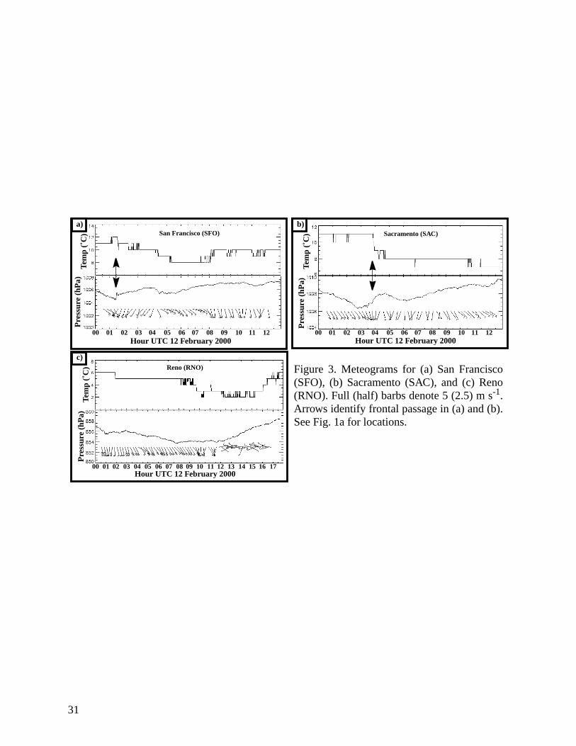
like a cold front. For example, as the occluded front moved across north-central California, 2–4˚C

surface temperature falls were observed at San Francisco (SFO, Fig. 3a) and Sacramento (SAC,

Fig. 3b), and radar imagery revealed that a narrow frontal rainband was coincident with the

occluded front and embedded within the large-scale precipitation shield (not shown). The

baroclinity of the occluded front weakened rapidly with height with little temperature contrast at

700 hPa (Fig. 2b). Southwesterly cross barrier flow produced a lee trough east of the Sierra

Nevada (Fig. 2d).

7

The vertical structure of the system was complex. Wind profiler observations near SFO at

Richmond (RMD) and SAC (see Fig. 1a for locations) indicated backing winds with height within

the low-level frontal zone, which sloped rearward with height (Figs. 4a and 4b). Above the low-

level frontal zone, however, the 0300 UTC (all times for 12 February 2000 unless noted) RUC2

analysis showed that the upper-level trough axis sloped forward with height from 600 hPa to 250

hPa, with the leading edge of a weak upper-level baroclinic zone downstream over western

Nevada (Fig. 5). The upper-level trough was accompanied by a significant relative humidity

gradient, with high relative humidities ahead and lower relative humidities behind. The strongest

and deepest upward vertical velocities were located downstream of the trough axis and beneath

the upper-level baroclinic zone.

By 0600 UTC, the primary 500-hPa vorticity maximum was positioned off the south-

central California coast (Fig. 6a), and a well-defined upper-level trough was evident in satellite

imagery (Fig. 6c). A large area of moderate to heavy precipitation was found over central

California and the Sierra, while lighter precipitation extended northeastward from north-central

Nevada towards southern Idaho (Fig. 6d). A secondary 500-hPa vorticity maximum (Fig. 6a),

associated with an upper-level jet streak (not shown), extended downstream across northeast

Nevada. As this vorticity maximum approached northern Utah, mid- and upper-tropospheric

relative humidities increased (e.g., 700 hPa, Fig. 6b). At 700 hPa, there was little or no

temperature advection over central California (Fig. 6b), however, wind profiler observations

suggested (Figs. 4a and 4b) that winds were backing with height below 700 hPa, indicating cold

advection below 700 hPa. The 1500-m low center had become more diffuse and was located over

southwest Oregon (Fig. 6d). The occluded front, which was now detached from the low center,

was approaching the windward slopes of the Sierra Nevada (Fig. 6d). Due to the higher mean

elevation of the Intermountain region, the remainder of this paper will define vertical levels as

follows: low-level from the surface to 700 hPa, mid-level 700–500 hPa, and upper-level above 500

hPa.

From 0600-1200 UTC, the surface front approached the Sierra Nevada and its

8

thermodynamic and kinematic structure became less coherent as it split around the Sierra Nevada

as observed during other events (e.g., Fig. 4.16, Blazek 2000). Specifically, the eastward

movement of the surface front was retarded by the central Sierra. The southern portion of the

occluded front was deflected equatorward while the northern portion continued eastward (refer to

summary Fig. 12a). The front weakened dramatically by the time it moved into the lee of the

Sierra. At Reno (RNO, see Fig. 1a for location), a station pressure minimum occurred around

0800 UTC with a 2°C temperature decrease between 0900–1000 UTC, which was coincident with

a trace of light rain from 0936–0946 UTC and veering winds from southeasterly to southerly (Fig.

3c). Winds then decreased and shifted to westerly as station pressures began to steadily rise

around 1200 UTC. Thus, there was a well-defined wind shift accompanied with a pressure rise at

RNO that featured little or no temperature change. The temperature drop preceeded the wind shift

and was coincident with light rain and presumably evaporative cooling. This evolution may be

related to RNO being immediately downstream of the Sierra Nevada; perhaps the deepest cold air

was blocked by the Sierra or never arrived due to downslope warming, while a precipitation band

associated with mid-level vertical motion was able to traverse the Sierra ahead of the large-scale

pressure trough.

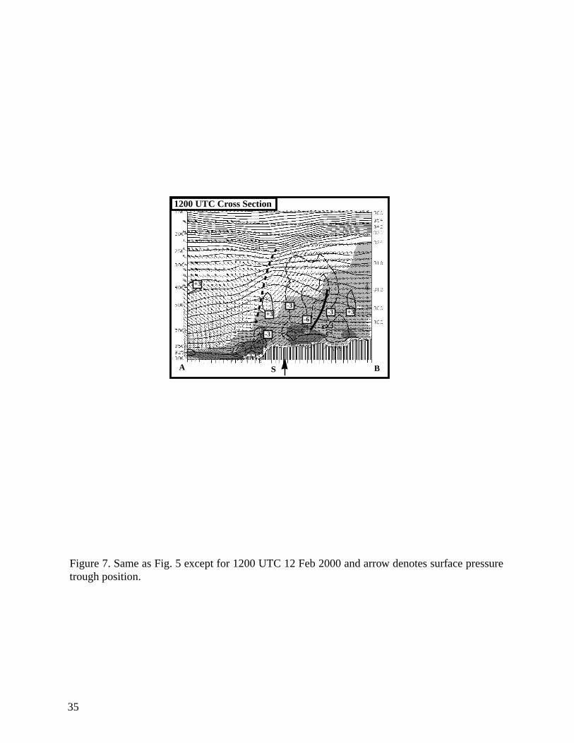
By 1200 UTC, the upper-level trough was located downstream of the Sierra Nevada crest

over western Nevada, and the upper-level baroclinic zone had weakened (Fig. 7). The upper-level

baroclinic zone, mid-level cold advection, and deep tropospheric vertical motion were moving

across Nevada and approaching northern Utah (cold advection not shown). Precipitation across

most of California had ended, and widespread precipitation was falling across much of the

Intermountain region, including the IPEX target area (not shown).

A curious aspect of this event was the rapid movement of the surface pressure trough

across Nevada. Between 1200–1800 UTC, the surface pressure trough moved rapidly (20–25 m s-

1) across Nevada, and generally featured veering surface winds and little or no surface baroclinity.

For example, when the surface pressure trough passed Elko (EKO, see Fig. 1a for location)

around 1400 UTC, winds were calm, surface temperatures remained steady at 2˚C, and light snow

9

was falling (not shown). The rapid movement was better correlated with the speed of the upper-

level trough axis rather than by low-level advection. In fact, the surface pressure trough was

nearly coincident with the leading edge of the upper-level trough and the deepest upward vertical

velocity (Fig. 8). Thus, the pressure minimum associated with the surface trough was most likely

a reflection of upper-level mass divergence and associated vertical motion immediately ahead of

the upper-level trough, as observed in other events over the western United States (e.g., Hess and

Wagner 1948; Schultz and Doswell 2000).

At 1800 UTC, the primary 500-hPa vorticity maximum was positioned over southern

Nevada, and the 500-hPa trough axis had elongated and split, becoming negatively tilted (Fig. 9a).

Although the strongest 500-hPa vorticity was located over southern Nevada, the primary surface

low pressure center was positioned well to the north, near the Idaho–Oregon border, with a

secondary pressure minimum over northwest Wyoming (Fig. 9d). The surface pressure trough,

along with widespread clouds and precipitation, was present ahead of and roughly parallel to the

500-hPa trough axis (Fig. 9c). At 700 hPa, higher relative humidity and weak cold advection was

generally present over the Intermountain region (Fig. 9b).

As the surface trough moved across northern Utah between 2000–2200 UTC, it developed

baroclinity, and will hereon be referred to as the baroclinic trough. Ahead of the baroclinic trough,

IPEX scientists were perplexed when mesoscale observations revealed a midlevel trough that

arrived ~3 h ahead of the baroclinic trough. The midlevel trough was not accompanied by an

abrupt change in temperature or moisture, but rather a small (1–3˚C over 2 h) decrease in

equivalent potential temperature with respect to ice (θei). The midlevel trough appeared to

develop along a high potential vorticity banner that developed over the southern Sierra Nevada.

Schär et al (2003) and (2004) describe the development of similar banners over the

Alps and Dinaric Alps. As shown in Figure 10, low and high potential vorticity banners extended

downstream from the Sierra at 0600 UTC (Fig. 10a). By 1200 UTC, the southwesterly flow had

advected the high potential vorticity banner northeastward into northeast Nevada and northwest

Utah (Fig. 10b). The weak mid-level trough appeared to develop along this high potential vorticity

Grubisic

10

banner as it moved downstream into the Great Salt Lake Basin (Fig. 10c).

By 0000 UTC 13 Feb, the 500-hPa trough had weakened considerably with the primary

vorticity maximum in northeast Arizona (Fig. 11a). A broad region of low 1500-m pressure

extended from the Idaho-Montana border southeastward to Wyoming with weak ridging building

over Utah (Fig. 11c). Weak 700-hPa cold advection (not shown), clouds and precipitation were

present over much of northern Utah (Figs. 11b and 11c), but the precipitation event was close to

ending.

Figure 12a and 12b summarize the surface and vertical structure evolution of this event.

An occluded mid-latitude cyclone made landfall around 0000 UTC 12 Feb 2000. As the system

moved inland, the low pressure area became increasingly diffuse, separated from the surface

occluded front, and moved northeastward while the surface occluded front advanced towards the

Sierra Nevada. The surface front sloped rearward with height, but the associated upper-level

trough was forward-sloping. As the system approached the Sierra, the surface front weakened and

split into northern and southern sections, while the upper-level trough and baroclinic zone

continued moving eastward. Essentially, the terrain acted to “strip” the low-level occluded front

from the upper-level trough. The upper-level trough then coupled with the Sierra lee trough, and

the two features moved rapidly downstream across northern Nevada. The rapid movement of the

surface trough suggested close coupling with the mass divergence accompanying the upper-level

trough. Over northern Utah, these features were preceded by a mid-level trough that formed along

a high potential vorticity banner that developed over the Sierra Nevada.

4. Mesoscale storm structure over northern Utah

a) Pre-baroclinic surface trough period 0900–2100 UTC

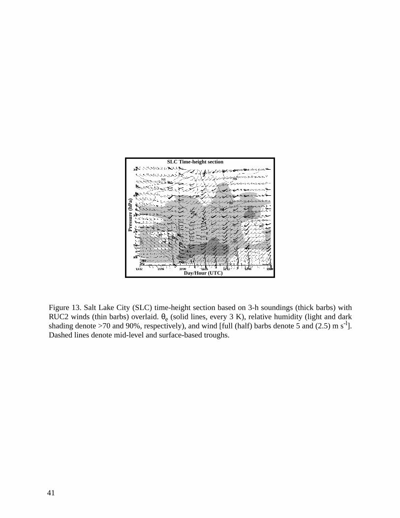
Southerly to southwesterly low- and mid-level flow developed over the IPEX target area as

the upper-level and surface troughs approached northern Utah. Between 0900–1800 UTC, there

was little change to the large-scale kinematic environment which featured southerly low-level

flow with an 8–12 m s-1 wind speed maximum located just below mid-mountain (hereafter

11

defined as 775 hPa or ~2200 m AMSL) at 800 hPa (Fig. 13). Above this level, winds veered to

southwesterly, resulting in a significant cross-barrier flow component at crest level (~700 hPa). In

the lowlands, winds were mainly southerly within the valleys upstream of the Wasatch Mountains

(Figs. 14a,b). This southerly along-barrier flow (hereafter referred to as valley flow) was oriented

normal to the 1500-m isobars (cf. Figs. 9d and 13b) and was highly ageostrophic. Southwesterly

flow over and upstream of the Great Salt Lake became confluent with the along-barrier flow near

the eastern shore of the Great Salt Lake. ADAS analyses showed that this region of confluent flow

was convergent (Fig. 15), and it will hereon be referred to as a windward convergence zone.

Precipitation began to fall at mountain locations by ~0900 UTC as the large-scale upward

vertical motion and moisture ahead of the upper-level trough overspread northern Utah (Fig. 16a).

Precipitation onset was delayed up to 3h at many lowland sites (e.g., SNX and SLC, Fig. 16b).

This delay appeared to be the result of low-level sublimation and evaporation as suggested by the

0600 and 1200 UTC soundings from SLC which showed a descending cloud base with the 775–

600 hPa lapse rate approaching the pseudo adiabat (Fig. 17). By 1200 UTC, vertical profiles of

potential temperature (θ) and equivalent potential temperature with respect to ice (θei) showed

that, with the exception of a shallow layer near 800 hPa,θ increased with height from the surface

to 500 hPa, butθei was nearly constant with height up to 575 hPa, indicating near-neutral stability

for ice-saturated ascent (Fig. 18a). By 1800 UTC, this near-neutral layer extended to ~500 hPa at

both near-barrier sounding locations (SLC and NSSL5, Figs. 18a,b).

Precipitation during this period was generally widespread with some weak convective

elements; 0.5˚ base reflectivities were no greater than 35dbz (e.g. Fig. 19a). Animation of radar

reflectivity showed some transient precipitation features, but by in large the precipitation was

fixed to the terrain. This suggested that precipitation processes were strongly influenced by the

regional orography. For example, radar imagery at 1900 UTC 12 Feb showed an area of locally

high reflectivity upstream of the Wasatch Mountains near OGD, whereas lower reflectivities

(often below 5 dBZ) were found over the Salt Lake Valley (Fig. 19b). Although beam blockage

and other radar limitations prevented analysis of the KMTX reflectivity structure directly over the

12

Wasatch Mountains, a narrow reflectivity maximum was observed directly over the barrier crest

by the NOAA WP-3D tail radar (see Cox et al. 2004).

Precipitation gauge observations from five northern Utah locations, including two

mountain sites (CLN and SNI) and three lowland sites (OGD, SNX, and SLC, see Fig. 1b for

locations), further illustrate the orographic influences on the precipitation distribution. Although

blocking of the large-scale southwesterly flow by the Wasatch and other ranges resulted in

southerly along-barrier flow at low levels (e.g., Fig. 14, Cox et al. 2004), sufficient (5–10 m s-1)

cross barrier flow at mid-mountain and crest level (Fig. 20, 1800 UTC traces) produced a

substantial orographic enhancement. By 2100 UTC, SNI and CLN reported 2.4 cm and 3.0 cm

SWE, respectively (Fig. 16c), with fairly constant precipitation rates reaching 4 mm h-1 (Fig.

16b). Precipitation at SNI (CLN) was roughly double (thirty) times that at nearby low elevation

OGD (SLC).

In the lowlands immediately upstream of the Wasatch Mountains, significant precipitation

contrasts were observed between OGD, SNX, and SLC. Only 0.1 cm of rain fell at SLC (surface

temperatures were 4–5˚C) through 2100 UTC, whereas Ogden (OGD) and Antelope Island

(SNX), which are located 30–40 km north of SLC and upstream of the northern Wasatch

mountains, recorded much more with 1.6 cm and 1.1 cm, respectively (Fig. 16a). At least two

factors contributed to this lowland precipitation contrast. One, the subcloud evaporation and rain

shadowing over the Salt Lake Valley, as discussed in the next paragraph; two, windward

convergence and precipitation enhancement in the vicinity of OGD.

Precipitation at OGD and SNX was coincident with a saturated low-level environment as

indicated on the 1800 UTC NSSL5 sounding (Fig. 21). In contrast, the 1800 UTC SLC sounding

revealed a much a drier low-level environment that likely reduced precipitation amounts at SLC.

The drier low-level environment at SLC, as well as across much of the Salt Lake Valley, appeared

to be partially related to downslope flow from the southern terminus of the Salt Lake Valley (e.g.,

Fig. 14b), which features a traverse mountain range that reaches more than 2000 m, and/or

subsidence produced by rainshadowing to the lee of the Oquirrh Mountains. The presence of a

13

pre-existing dry environment (Fig. 17) also played a role.

Heavier precipitation was observed at OGD and SNX (Figs. 16b,c), which were not

strongly influenced by rainshadowing from upstream ranges. These sites were affected also by the

windward convergence zone, which enhanced precipitation over the lowlands immediately

upstream of the Wasatch Mountains. As illustrated by Figs. 14 and 15, convergence was observed

upstream of the Wasatch Mountains where southwesterly flow merged with southerly along-

barrier flow. The most significant precipitation enhancement occurred immediately downstream

of the convergence zone, as illustrated by the region of high radar reflectivity extending

approximately 25 km upstream of the Wasatch Crest near Ogden at 1900 UTC (Fig. 19b).

Precipitation rates at OGD reached 2.5 mm SWE h-1, which was at times surprisingly similar to

the nearby mountain precipitation rate at SNI (cf. Figs. 15a,b). The convergence zone and

associated windward precipitation region advanced toward the barrier with the approach of the

baroclinic trough, as described in detail by Cox et al. (2004) and Colle et al. (2004).

The storm environment was modified only slightly as the midlevel trough moved across

northern Utah between 1800–2100 UTC (Fig. 13). The midlevel trough was marked by veering

winds between 700 and 500 hPa. P-3 flight-level data between 700 hPa and 500 hPa revealed there

were no abrupt temperature or moisture gradients present across the midlevel trough, but rather a

small (1–3˚C over 2 h) decrease of mid- and upper-levelθei. No organized precipitation structures

were coincident with the midlevel trough, although the confluent flow over the eastern half of the

Great Salt Lake advanced toward the Wasatch Mountains during and following its passage (see

Cox et al. 2004). During this period, lowland precipitation rates increased slightly or remained

steady, but at most mountain stations (1900m ASL and above), precipitation rates remained

steady or decreased slightly.

b) Postbaroclinic trough period 2100-0600 UTC

At 2100 UTC, the surface baroclinic trough was collocated with a weak east-west band of

precipitation over the southern end of the Great Salt Lake (Fig. 19c). The baroclinic trough

14

intensified as it moved across northern Utah, and, at SLC, was accompanied by a 2˚C temperature

drop, surface pressure minimum, and wind shift around 2130 UTC (Fig. 22). The strongest

temperature changes with the baroclinic trough over northern Utah were coincident with moderate

or heavy precipitation; thus, diabatic processes appeared to produce much of the baroclinity

accompanying the trough as it moved into northern Utah, similar to that described by Schultz and

Trapp (2003).

The wind changes accompanying the baroclinic trough were complex across northern

Utah. At DPG and the immediately adjacent lowlands, surface winds veered from southerly to

westerly with baroclinic trough passage (cf. Fig. 14b, Fig. 23). Across the Salt Lake and Tooele

Valleys, however, the surface wind shift was weak, or short-lived (Fig. 23), with a few exceptions

(e.g., SLC, Fig. 22). Inspection of MesoWest stations around 800 m above valley level, however,

revealed that a consistent wind shift was associated with the baroclinic trough just above valley

level. This elevated wind shift was continuous, moved east-southeast (confirmed with KMTX

velocity data, not shown), and was also coincident with the largest temperature falls, which were

2–4˚C between 800–600 hPa, with the most significant drop being 4˚C at 650 hPa over 2h. Thus,

the most notable temperature and wind direction changes associated with the baroclinic trough

were generally elevated, between 800 and 600 hPa, and not at valley level.

Precipitation behind the baroclinic trough grew more convective as the low-levels became

increasingly unstable after baroclinic trough passage. Much of the lowland precipitation was

associated with two transient mesoscale precipitation areas, one a weakly organized area

associated with the baroclinic trough (Fig. 19c), and the second a convective line that passed SLC

and produced a 4˚C temperature drop about 3 h later (Fig. 22). In fact, turbulence and wind shear

accompanying this feature (not shown) were strong enough to abort the P-3’s first landing

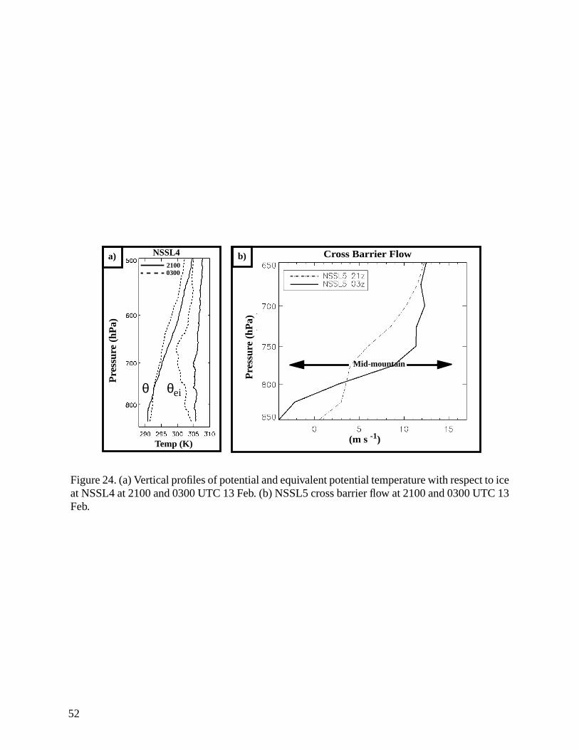
attempt. The convective line developed in the airmass behind the baroclinic trough, which

featuredθei decreasing with height up to 675 hPa (Fig. 24a). As the baroclinic trough moved

southeast, lowland precipitation rates spiked at different times: OGD around 2100 UTC, SNX at

2200 UTC and SLC at 0000 UTC 13 February (Fig. 16c). Precipitation rates at mountain sites,

15

however, peaked after the lowland locations, reaching 4 mm hr-1 at both SNI and CLN between

0000–0100 UTC 13 February (Fig. 16b); these increased mountain precipitation rates were

associated with destabilization and increased cross-barrier flow behind the baroclinic trough (Fig.

24b), but also could be a reflection of snow buildup on gauge walls falling into the bottom of the

gauge, as discussed in Cox et al. (2004). Precipitation enhancement that previously accompanied

the windward convergence zone over the lowlands upstream of the northern Wasatch (e.g., OGD,

SNX) ended shortly after passage of the baroclinic trough.

Across the Salt Lake and Tooele Valleys, much of total storm precipitation fell in the

postbaroclinic trough environment (e.g., SLC 83%) under northwesterly flow when low-level

moisture and instability were maximized. Precipitation at mountain locations, however, was

generally evenly distributed throughout the event with CLN and SNI receiving about 40% of their

total SWE in the postbaroclinic trough environment. Precipitation at both mountain and valley

locations ended by 0600 UTC 13 February, as a drier environment and subsidence behind the

upper-level trough developed.

c) Analysis of Orographic Precipitation

Storm-total SWE ratios featured three main spatial precipitation patterns. One, significant

precipitation enhancement was observed in the higher elevations. Second, precipitation

suppression was observed both to the lee of the Wasatch and Oquirrhs mountains, including the

Salt Lake and Tooele Valleys. Third, local precipitation enhancement was observed in the

lowlands upstream of the northern Wasatch (Fig. 25a).

Precipitation generally increased with altitude in IOP3 (Fig. 25b), which resembled the

nearly linear climatological distribution (Fig. 25c). However, unlike the climatological

precipitation distribution, IOP3 featured a somewhat bimodal distribution above and below

2100m or at lowland and mountain locations. This bimodal precipitation distribution suggested

that significant variations from climatological precipitation versus altitude were present during

IOP3. Some of these departures from climatology could be explained by two observed spatial

16

precipitation patterns: one, precipitation suppression in the lee of the Oquirrh mountains (e.g.,

SLC), and two, precipitation enhancement in the lowlands upstream of the northern Wasatch (e.g.,

SNX, OGD). For example, SNX and SLC, which have a similar elevation (1280m), orientation

relative to the Wasatch, and climatological annual precipitation (SNX, 45.6 cm, SLC, 42 cm),

featured nearly a factor of three SWE difference, SNX (1.5 cm) and SLC (.6 cm). Mountain sites

(e.g., SNI, 2256m, 4.9 cm) over the northern Wasatch also featured greater precipitation for their

respective elevation compared to CLN (2945m, 5.1 cm).

Precipitation anomaly maps were constructed to further compare climatological and IOP3

spatial precipitation patterns. Since annually averaged precipitation correlates well with altitude

over the IPEX target region (Fig. 25c), a linear regression equation was developed to describe the

climatological precipitation altitude relationship and is given byP = 0.0523*A–30.406, whereP is

the precipitation in cm andA is the altitude in meters. Analysis of the residuals or anomalies from

this predicted value for climatological precipitation are shown in Fig. 26a. Positive anomalies are

relatively wet areas for their respective elevations, and include the northern Wasatch mountains,

lowlands immediately upstream of the Wasatch, eastern two thirds of the Great Salt Lake, and the

northern and eastern Tooele and Salt Lake Valleys (Fig. 26a). Negative anomalies, or areas that

are relatively dry for their respective elevations, are present over the Great Salt Lake desert,

southern Oquirrh Mountains, and downstream of the Wasatch crest (Fig. 26a).

In order to illustrate departures from the climatological precipitation-altitude relationship

during IOP3, the slope of the climatological linear fit was fixed to the IOP3 mean precipitation,

with residuals from this line presented in Figure 26b. IOP3 generally featured similar

precipitation anomaly patterns to climatology, including positive (wet) anomalies over and

upstream of the northern Wasatch and negative (dry) anomalies east of Wasatch (Fig. 26b).

However, there were differences between IOP3 and climatological precipitation anomaly patterns

over the Salt Lake and Tooele Valleys, where the precipitation amounts were smaller than one

would expect climatologically.

17

5. Discussion

a) Storm evolution over the western United States

Very few studies have examined the evolution of a winter storm from the Pacific Coast to

the interior Intermountain West. During IPEX IOP3, a landfalling occluded front weakened and

deformed as it approached the Sierra Nevada, similar to that observed previously near the Sierra

Nevada by Hoffman (1995), Reynolds and Kuciasuskas (1988), and Blazek (2000), as well as

upstream of the Appalachians (Schumacher et al. 1996). Ultimately, there was little evidence that

the baroclinity associated with the surface based occlusion was able to penetrate into the lowlands

to the lee of the Sierra Nevada as the upper-level trough continued to move downstream. Thus, the

high topography appeared to "strip" or remove the storm system of its low-level baroclinic

structure as it traversed the Sierra Nevada. Destruction of the low-level baroclinity may have also

been aided by adiabatic warming to the lee of the Sierra Nevada, as suggested by Hobbs et al.

(1996) for frontal evolution in the lee of the Rocky Mountains.

To the lee of the Sierra, the upper-level trough interacted with the lee trough, which

became mobile and moved rapidly downstream as the upper-level trough axis approached. The

downstream movement of the surface trough appeared to be a reflection of mass-divergence

associated with the upper-level trough, consistent with early work by Hess and Wagner (1948)

and Schultz and Doswell (2000).

The scenario described above suggests that the low-level occluded front and associated

pressure trough did not move continuously across the Sierra Nevada. Instead, the occluded front

was blocked by the Sierra Nevada while the upper-level trough moved downstream and interacted

with the lee trough. This evolution contrasts with that of many idealized simulations of fronts

traversing topography (see Blumen 1992 and Egger and Hoinka 1992 for reviews), which

typically assume smooth slopes and modest relief so that the front is able to surmount the

mountain barrier. It is, however, roughly consistent with the discontinuous low-level evolution

described by Dickinson and Knight (1999) who found that for high mountains, the low-level front

is blocked, while the associated upper-level potential vorticity maximum moves downstream and

18

eventually couples with the leeward low-level cyclonic vorticity maximum.

Another curious aspect of IOP3 is the forward-sloping structure of the upper-level trough.

This structure resembles that of damping baroclinic waves (e.g., Spencer et al. 1996) and is

consistent with the fact that the cyclone was occluded and weakening as it began to interact with

the terrain of the western United States.

Finally, the analysis presented in section 4 illustrates a likely origin of the mid-level

trough that perplexed IPEX scientists during IOP3 (Schultz et al. 2002). Southwesterly flow ahead

of the approaching storm system produced high and low potential vorticity banners downstream

of the southern and northern Sierra Nevada, respectively. These banners were qualitatively similar

to potential vorticity banners that form downstream of the European Alps (e.g., Schär et al. 2003,

2004). The mid-level trough formed along the high potential vorticity banner as it was

advected downstream into northeast Nevada and then eastward into Utah. Thus, it appears that

potential vorticity banners that form over the Sierra Nevada may complicate the kinematic

structure of winter storms over Nevada and Utah. In this case, however, the mid-level trough

appeared to have little effect on precipitation processes.

b) Precipitation distribution over northern Utah

In general, there is a strong correlation between climatological precipitation and altitude

across the Intermountain West. As such, precipitation-altitude relationships are used frequently by

meteorologists and hydrologists to predict event or annual precipitation (e.g., Hevesi et al. 1992).

Over the IPEX target region, climatological precipitation increases linearly with height (e.g.,

Alter 1919; Daly et al. 1994; Fig. 25c) with a linear correlation coefficient of 0.70. Large

departures from this relationship have been observed, however, for storm total precipitation (e.g.,

Horel and Gibson 1994; Cheng 2001; Shafer et al. 2002) and within individual storms (e.g.,

Steenburgh 2003). In addition, as illustrated by Fig. 26a and Peck and Brown (1962), the northern

Wasatch Mountains and their immediate upstream lowlands, the eastern two-thirds of the Great

Salt Lake, and the northern and eastern Tooele and Salt Lake Valleys are anomalously wet for

Grubisic

19

their elevations, whereas the Great Salt Lake Desert and areas east of the Wasatch Mountains are

anomalously dry. Therefore, in addition to a pronounced precipitation-altitude relationship, there

are important mesoscale patterns evident in the regional precipitation climatology.

Precipitation during IOP3 occurred under moist southwesterly flow with near moist-

neutral stability. Precipitation was dominated by local terrain processes, which produced

enhanced/suppressed precipitation at various locations across northern Utah. Three major

precipitation patterns were observed: (1) precipitation enhancement with increased altitude, (2)

precipitation suppression in the lee of the Stansbury and Oquirrh Mountains (i.e., the Tooele and

Salt Lake Valleys), and (3) precipitation enhancement produced by a windward convergence zone

over the lowlands upstream of the northern Wasatch Mountains.

These patterns featured important similarities and differences compared to climatology.

Precipitation enhancement in the northern Wasatch Mountains and upstream lowlands was

consistent with this region being climatologically wet for its elevation. In contrast, IOP3 was dry

relative to climatology over the Salt Lake and Tooele Valleys. These characteristics are consistent

with southwesterly flow events based on synoptic experience.

Analyses of departures from climatological precipitation-altitude relationships should be

employed to better understand event, seasonal, and long-term precipitation distributions in regions

of complex terrain. The construction of precipitation anomaly maps for varying flow directions

and stability may be a useful predictive tool since systematic precipitation anomalies can be more

easily identified and may help expose the underlying processes responsible for such anomalies.

Such anomaly maps may also be useful for bias-correcting numerical model forecasts and would

likely improve upon techniques that rely primarily on the climatological precipitation-altitude

relationship.

6. Summary and Conclusions

This paper has examined the evolution of a winter storm (IPEX IOP3) over the western

United States and its precipitation distribution over northern Utah. The event featured a land-

20

falling occluded front that weakened and deformed as it approached the Sierra Nevada. The

occluded front was unable to surmount the Sierra Nevada as the accompanying forward-sloping

upper-level trough moved downstream. This apparent terrain stripping of the low-level frontal

structure, combined with the coupling of the upper-level trough with the Sierra Nevada lee trough,

represents a discontinuous low-level storm evolution that is roughly consistent with the idealized

modeling work of Dickinson and Knight (1999). Eventually, the lee trough moved rapidly

downstream and appeared to be a reflection of the mass-divergence downstream of the upper-level

trough axis.

As the upper-level trough approached northern Utah, it interacted with a mid-level trough

that was associated with a high potential vorticity banner that formed downstream of the southern

Sierra Nevada. This produced the complex kinematic structure that perplexed IPEX scientists

during IOP3. The passage of the mid-level trough across northern Utah, however, had a limited

effect on precipitation processes.

Precipitation during the event was dominated by mesoscale terrain processes and featured

a general pattern of increased precipitation with increased altitude. Two important departures

from the general precipitation-altitude relationship where found: one, the northern Wasatch

Mountains and accompanying lowlands were anomalously wet (the development of a windward

convergence zone contributed to the lowland enhancement as described by Cox et al. 2004); two,

the Tooele and Salt Lake Valleys were anomalously dry. Analyses of long-term and event-specific

departures from the climatological precipitation-altitude relationship illustrated that the former

was consistent with climatological precipitation distributions, whereas the latter was not.

Widespread use of analyses that illustrate long-term and event-specific departures from

climatological precipitation-altitude relationships may prove useful for bias-correcting numerical

model forecasts and identifying important mesoscale precipitation patterns that are difficult to

identify due to the dominance of altitudinal gradients.

This study represents a rare investigation of winter storm evolution over the western

United States. During IOP3, the upper-level trough was able to move relatively unimpeded across

21

the Sierra Nevada and Great Basin ranges while the low-level occluded front was fully blocked,

which resulted in discontinuous low-level storm evolution. These observations could be broadly

applied to similar events that feature a landfalling mature midlatitude cylone in California and

move across the Intermountain region as the accompanying baroclinic wave weakens. Namely,

low-level structures of midlatitude cyclones across the Intermountain region are strongly

dependent upon interactions with the underlying terrain, while upper-level features move more or

less unimpeded by the complex underlying terrain. Also, mesoscale, terrain-induced circulations

dominated precipitation distribution across northern Utah and included not only direct orographic

ascent where more precipitation fell in higher terrain, but also enhanced/suppressed precipitation

in nearby lowland areas.

This study illustrates the importance of the Intermountain West’s topography on synoptic

storm evolution and precipitation. Additional research is needed to better understand the passage

of baroclinic systems across the Sierra Nevada, including how the resulting terrain-modified

structure affects the development and evolution of precipitation over the downstream

Intermountain West.

Acknowledgments.Funding for the analysis of IPEX IOP3 was provided by National

Science Foundation Grants ATM-0085318 and ATM-0333525, and a series of grants provided by

the National Weather Service C-STAR program to the NOAA Cooperative Institute for Regional

Prediction at the University of Utah. Comments from Lance Bosart and David Schultz improved

this paper. We would like to thank all the individuals and organizations who participated in the

planning and execution of IPEX. Thanks to the National Severe Storms Lab for operating the

mobile labs and the National Weather Service for supplementing radiosonde observations. Thanks

also to David E. White and Paul Neiman of NOAA’s Environmental Technology Laboratory

(ETL) for providing the California wind profiler data.

22

References

Alter, J. C., 1919: Normal precipitation in Utah.Mon. Wea. Rev., 47, 633-636.

Baer, V. E., 1991: The transition from the present radar dissemination system to the NEXRAD

Information Dissemination Service (NIDS).Bull. Amer. Meteor. Soc., 72, 29-33.

Benjamin, S. G., J. M. Brown, K. J. Brundage, B. E. Schwartz, T. G. Smirnova, T. L. Smith and L.

L. Marone, 1998: RUC-2 –The Rapid Update Cycle Version 2. NWS Technical Procedue

Bulletin No. 448. NOAA/NWS, 18 pp. [Available from National Weather Service, Office

of Meteorology, 1325 East-West Highway, Silver Spring, MD 20910].

Blazek, T. R., 2000: Analysis of a Great Basin cyclone and attendant mesoscale features. M.S.

thesis, Dept. of Meteorology, University of Utah, 122 pp. [Available from Dept. of

Meteorology, University of Utah, 145 South 1460 East, Room 819, Salt Lake City, UT

84112-0110.]

Bluestein, H. B., 1986: Fronts and jet streaks: A theoretical perspective.Mesoscale Meteorology

and Forecasting. (P. S. Ray, Ed.), Amer. Meteor. Soc., 173-215.

Blumen, W., 1992: Propagation of fronts and frontogenesis versus frontolysis over orography.

Meteor. Atmos. Phys., 48, 37-50.

Cheng, L., 2001: Validation of quantitative precipitation forecasts during the Intermountain

Precipitation Experiment. M.S. thesis, Dept. of Meteorology, University of Utah, 137 pp.

[Available from Dept. of Meteorology, University of Utah, 145 South 1460 East, Rm. 819,

Salt Lake City, UT 84112-0110.]

Colle, B. A., J. B Wolfe, W. J. Steenburgh, D. E. Kingsmill, J. A. W. Cox, and J. C. Shafer, 2004:

High resolution simulations and microphysical validation of an orographic precipitation

event over the Wasatch Mountains during IPEX IOP3. Submitted toMon. Wea. Rev.

Cox, J. A.W, W. J. Steenburgh, D. E. Kingsmill, J. C. Shafer, B. A. Colle, O. Bousquet, B. F.

Smull, and H. Cai, 2004: The kinematic structure of a Wasatch Mountain winter storm

during IPEX IOP3.Mon. Wea. Rev. In press.

Daly, C., R. P. Neilson, and D. L. Phillips, 1994: A statistical-to-topographic mode for mapping

23

climatological precipitation over mountainous terrain.J. Appl. Met., 33, 140-158.

Dickinson, M. J., D. Knight, 1999: Frontal interaction with mesoscale topography.J. Atmos. Sci.,

56, 3544-3559.

Egger, J., and K. P. Hoinka, 1992: Fronts and orography.Meteor. Atmos. Phys., 48, 3-36.

Elliott, R. D., 1958: California storm characteristics and weather modification.J. Meteor.15, 486-

493.

, V., 2004: Bora-driven potential vorticity banners over the Adriatic.Quart. J. Roy. Met.

Soc., 130, 2571-2603.

Hess, S. L., and H. Wagner, 1948: Atmospheric waves in the northwestern United States.J.

Meteor., 5, 1-19.

Hevesi, J. A., A. L. Flint, and J. D. Istok, 1992: Precipitation estimation in mountainous terrain

using multivariate geostatistics. Part II: Isohyetal Maps.J. Appl. Meteor., 31, 677-688.

Hobbs, P.V., J.D. Locatelli, and J. E. Martin, 1996: A new conceptual model for cyclones

generated in the lee of the Rocky Mountains.Bull. Amer. Meteor. Soc., 77, 1169-1178.

Hoffman, E. G., 1995: Evolution and mesoscale structure of fronts in the western United States: A

case study. M.S. thesis, Dept. of Earth and Atmospheric Sciences, State University of New

York at Albany, 287 pp.

Horel, J. D., and C. V. Gibson, 1994: Analysis and simulation of a winter storm over Utah.Wea.

Forecasting, 9, 479-494.

Horel, J. D., M. Splitt, L. Dunn, J. Pechmann, B. White, C. Ciliberti, S. Lazarus, J. Slemmer, D.

Zaff, and J. Burks, 2002: Mesowest: Cooperative mesonets in the western United States.

Bull. Amer. Meteor. Soc., 83, 211-225.

Keyser, D., 1986: Atmospheric fronts: An observational perspectives.Mesoscale Meteorology

and Forecasting. (P. S. Ray, Ed.), Amer. Meteor. Soc., 216-258.

Lazarus, S. M., C. M. Ciliberti, J. D. Horel and K. A. Brewster, 2002: Near-real-time applications

of a mesoscale analysis system to complex terrain.Wea. Forecasting, 17, 971-1000.

Grubisic

24

NCDC, 2000:Storm Data. Vol. 42, No. 2, 127 pp.

Peck, E. L., and M. J. Brown, 1962: An approach to the development of isohyetal maps for

mountainous areas.J. Geophys. Res., 67, 681-694.

Reynolds, D. W., and A. P. Kuciauskas, 1988: Remote and in situ observations of Sierra Nevada

winter mountains clouds: Relationship between mesoscale structure, precipitation and

liquid water.J. Appl. Meteor., 27, 140-156.

Sanders, F., 1999: A proposed method of surface map analysis.Mon. Wea. Rev., 127, 945-955.

Schär, C., M. Sprenger, D. Lüthi, Q. Jiang, R. B. Smith, and R. Benoit, 2003: Structure and

dynamics of an Alpine potential-vorticity banner.Quart. J. Roy. Met. Soc., 129, 825-855.

Schultz, D. M., and C. A. Doswell III, 2000: Analyzing and forecasting Rocky Mountain lee

cyclogenesis often associated with strong winds.Wea. Forecasting, 15, 152-173.

Schultz, D. M., W. J. Steenburgh, R. J. Trapp, J. Horel, D. E. Kingsmill, L. B. Dunn, W. D. Rust,

L. Cheng, A. Bansemer, J. Cox, J. Daugherty, D. P. Jorgensen, and J. Meitín, L. Showell,

B. F. Smull, K. Tarp, and M. Trainor, 2002: Understanding Utah winter storms: The

Intermountain Precipitation Experiment.Bull. Amer. Meteor. Soc., 83, 190-210.

Schultz, D. M, and R. J. Trapp, 2003: Nonclassical cold-frontal structure caused by dry subcloud

air in northern Utah during the Intermountain Precipitation Experiment (IPEX).Mon.

Wea. Rev., 131, 2222-2246.

Schumacher, P. N., D. J. Knight, and L. F. Bosart, 1996: Frontal interaction with the Appalachian

Mountains. Part I: A climatology.Mon. Wea. Rev., 124, 2453-2468.

Shafer, J. C., 2002: Synoptic and mesoscale structure of a Wasatch Mountain winter storm. M. S.

thesis, Dept. of Meteorology, University of Utah, 65 pp. [Available from Dept. of

Meteorology, University of Utah, 135 South 1460 East, Rm. 819, Salt Lake City, UT

84112-0110]

Spencer, P. L., Carr, F. H., and Doswell, C. A. 1996: Diagnosis of an amplifying and decaying

baroclinic wave using wind profiler data.Mon. Wea. Rev., 124, 209-223.

Splitt, M. E., and J. D. Horel, 1998: Use of multivariate linear regression for meteorological data

25

analysis and quality assessment in complex terrain. Preprints,10th Symposium on

Meteorological Observations and Instrumentation, Phoenix AZ, Amer. Meteor. Soc., 359-

362.

Steenburgh, W. J., and T. R. Blazek, 2001: Topographic distortion of a cold front over the Snake

River Plain and central Idaho Mountains.Wea. Forecasting, 16, 301-314.

Steenburgh, W. J., 2003: One hundred inches in one hundred hours: Evolution of a Wasatch

Mountain winter storm cycle.Wea. Forecasting, 18, 1018-1036.

Stewart, J. Q., C. D. Whiteman, W. J. Steenburgh, and X. Bian, 2002: A climatological study of

thermally driven wind systems of the U.S. Intermountain West.Bull. Amer. Meteor. Soc.,

83, 699-708.

Westrick, K. J., C. F. Mass, and B. A. Colle, 1999: The limitations of the WSR-88D radar network

for quantitative precipitation measurement over the coastal western United States.Bull.

Amer. Meteor. Soc., 80, 2289-2298.

Wood, V. T., R. A. Brown, and S. V. Vasiloff, 2003: Improved detection using negative elevation

angles for mountaintop WSR-88Ds. Part II: simulations of the three radars covering Utah.

Wea. Forecasting, 18, 393-403.

26

Figure Captions

Figure 1. Topography and major geographic features of (a) the western United States and (b)

northern Utah. Elevation (m) based on scale at lower left in (a). Boxed area in (a) identifies

location of IPEX target area in (b).

Figure 2. Upper-level, satellite, surface, and radar analyses at 0000 UTC 12 Feb 2000. (a) RUC2

analysis of 500-hPa geopotential height (every 60 m) and absolute vorticity (x10-5 s-1,

shaded following scale at bottom). (b) RUC2 analysis of 700-hPa temperature (every 2˚C),

wind [full (half) barbs denote 5 (2.5) m s-1], and relative humidity (%, shaded following

scale at bottom). (c) Infrared satellite image. (d) NEXRAD radar mosaic (reflectivity scale

at left) and manual 1500-m pressure analysis. Station reports include 1500-m pressure

(tenths of hPa with leading 8 truncated), and wind [as in (b)].

Figure 3. Meteograms for (a) San Francisco (SFO), (b) Sacramento (SAC), and (c) Reno (RNO).

Full (half) barbs denote 5 (2.5) m s-1. Arrows identify frontal passage in (a) and (b). See

Fig. 1a for locations.

Figure 4. Wind profiler data for 12 February 2000 from (a) Richmond (RMD) and (b) Sacramento

(SAC). Full (half) barb denote 5 (2.5) m s-1. Meridional wind component plotted every 3

m s-1 as solid lines. Dashed lines denote wind shear accompanying frontal zone. See Fig.

1a for locations.

Figure 5. RUC2 cross section along line AB of Fig. 2b at 0300 UTC 12 Feb. Potential temperature

(thin lines every 3K), vertical velocity(ω, thick lines every 3x10-1 Pa s-1 with negative

contours dashed), wind [full (half) barbs denote 5 (2.5) m s-1], and relative humidity (light,

dark shading denote >70 and 90%, respectively). Upper-level trough axis denoted by

heavy dashed line, leading edge of upper-level baroclinic zone denoted by heavy solid

line, and surface front position denoted by arrow. Sierra Nevada indicated by S.

Figure 6. Same as Fig. 2 except for 0600 UTC 12 Feb 2000.

Figure 7. Same as Fig. 5 except for 1200 UTC 12 Feb 2000 and arrow denotes surface pressure

trough position.

27

Figure 8. Same as Fig. 5 except for 1800 UTC 12 Feb 2000 and arrow denotes position of surface

pressure trough.

Figure 9. Same as Fig. 2 except for 1800 UTC 12 February 2000.

Figure 10. EDAS 700-hPa potential vorticity (every 1x10-7 m2 s-1 K kg-1) and wind (vector scale

at lower right). High (low) potential vorticity banners denoted by thick solid (dashed) line.

(a) 0600 UTC 12 Feb 2000. (b) 1200 UTC. (c) 1800 UTC.

Figure 11. Same as (a) Fig. 2a, (b) Fig. 2c, and (c) Fig. 2d, except for 0000 UTC 13 Feb 2000.

Figure 12. Summary of surface and vertical structure evolution of IOP3. (a) Surface features every

3 h (conventional symbols) from 0000–2100 UTC 12 Feb 2000. Labels represent hour

UTC. (b) Vertical trough structure (roughly along line AB of Fig. 2b) every 3 h. U denotes

upper level trough, S surface trough, and M midlevel trough.

Figure 13. Salt Lake City (SLC) time-height section based on 3-h soundings (thick barbs) with

RUC2 winds (thin barbs) overlaid.θe (solid lines, every 3 K), relative humidity (light and

dark shading denote >70 and 90%, respectively), and wind [full (half) barbs denote 5 and

(2.5) m s-l]. Dashed lines denote mid-level and surface-based troughs.

Figure 14. Northern Utah manual streamline analysis at (a) 1200 and (b) 1800 UTC 12 Feb 2000.

Station data and streamlines for elevations between 1280–2200m AMSL (roughly at and

below mid mountain). Full (half) barbs denote 5 (2.5) m s-1.

Figure 15. ARPS Data Assimilation System (ADAS) surface analysis at 1800 UTC 12 Feb 2000,

surface divergence (light and dark shading denote less than -.25x10-4 s-1 and -3.0x10-4 s-1,

respectively) and wind [full (half) barbs denote 5 (2.5) m s-1].

Figure 16. Precipitation rates and accumulated precipitation at selected locations. (a) Mountain

precipitation rates (mm h-1). (b) Lowland precipitation rates (mm h-1). (c) Accumulated

precipitation (mm). See Fig. 1b for locations.

Figure 17. SkewT–logp diagram [temperature (solid) and dewpoint (dashed)] at SLC for 0600

UTC (black) and 1200 UTC (gray) 12 Feb 2000.

Figure 18. Vertical profiles of potential (left) and equivalent potential temperature with respect to

28

ice (right) at (a) SLC and (b) NSSL5. See Fig. 1b for locations.

Figure 19. Base (0.5˚) radar reflectivity from Promontory Point (KMTX) at (a) 1200 UTC 12 Feb,

(b) 1900 UTC 12 Feb, and (c) 2100 UTC 12 Feb 2000. Reflectivity scale (dBZ) on right.

Dashed line in (c) denotes position of baroclinic trough.

Figure 20. Cross-barrier flow magnitude (m s-1) at NSSL4 and NSSL5 for 1800 and 2100 UTC 12

Feb 2000. See Fig. 1b for locations.

Figure 21. SkewT–logp diagram [temperature (solid) and dewpoint (dashed)] at SLC and NSSL5

for 1800 UTC 12 Feb 2000.

Figure 22. Same as in Fig. 3 except for SLC. Arrows denote the passage of the baroclinic trough

(dashed) and convective line (solid). See Fig. 1b for location.

Figure 23. Same as Fig. 14 except for 2200 UTC 12 Feb 2000.

Figure 24. (a) Vertical profiles of potential and equivalent potential temperature with respect to ice

at NSSL4 at 2100 and 0300 UTC 13 Feb. (b) NSSL5 cross barrier flow at 2100 and 0300

UTC 13 Feb.

Figure 25. IOP3 precipitation characteristics. (a) Total accumulated liquid precipitation during

IOP3 (every 10 mm) with observations annotated; selected contour lines omitted for

clarity. (b) Observed liquid precipitation (cm) versus elevation over the IPEX target area.

(c) Climatological liquid precipitation (cm) versus altitude over the IPEX target area.

Figure 26. Climatological and observed precipitation anomalies. (a) Climatological precipitation

anomaly (cm) relative to linear fit. (b) IOP3 observed precipitation anomaly (mm) relative

to the slope of a linear fit to climatological precipitation versus altitude given in Fig. 25c.

Selected contour lines omitted for clarity.

29

Figures

Figure 1. Topography and major geographic features of (a) the western United States and (b)northern Utah. Elevation (m) based on scale at lower left in (a). Boxed area in (a) identifies loca-tion of IPEX target area in (b).

Sierra N

evadaInterm

ountain Region1500200025003000

500

SACRMD. . RNO.

N

300km

a)

SFO.Salt Lake

ValleyTooeleValley

.

SLC

Northern W

asatch

NSSL4NSSL5

DPG30km

N

Oquirrh M

ountains

Stansbury M

ountains

Great Salt Lake Basin

Great S

alt Lake

KMTX

OGDSNI

CLN

..

....

.

b)

Central W

asatch

30

L

40

40

38

38

4242

42

44

46

48

40

38

4244

46

48

a) 0000 UTC 12 Feb

Figure 2. Upper-level, satellite, surface, and radar analyses at 0000 UTC 12 Feb 2000. (a) RUC2analysis of 500-hPa geopotential height (every 60 m) and absolute vorticity (x10-5 s-1, shaded fol-lowing scale at bottom). (b) RUC2 analysis of 700-hPa temperature (every 2˚C), wind [full (half)barbs denote 5 (2.5) m s-1], and relative humidity (%, shaded following scale at bottom). (c) Infra-red satellite image. (d) NEXRAD radar mosaic (reflectivity scale at left) and manual 1500-m pres-sure analysis. Station reports include 1500-m pressure (tenths of hPa with leading 8 truncated), andwind [as in (b)].

5

15

25

35

45

55

A

B..

c) 0000 UTC 12 Feb

b) 0000 UTC 12 Feb

d) 0000 UTC 12 Feb

31

Figure 3. Meteograms for (a) San Francisco(SFO), (b) Sacramento (SAC), and (c) Reno(RNO). Full (half) barbs denote 5 (2.5) m s-1.Arrows identify frontal passage in (a) and (b).See Fig. 1a for locations.

San Francisco (SFO)

Tem

p (˚

C)

Pre

ssur

e (h

Pa)

Hour UTC 12 February 200000 01 02 03 05 06 07 08 09 10 11 1204

a)

Tem

p (˚

C)

Pre

ssur

e (h

Pa)

Hour UTC 12 February 200000 01 02 03 05 06 07 08 09 10 11 1204

b)Sacramento (SAC)

Tem

p (˚

C)

Pre

ssur

e (h

Pa)

Hour UTC 12 February 200000 01 02 03 05 06 07 08 09 10 11 1204

c)Reno (RNO)

13 14 15 16 17

32

Sacramento (SAC)b)

Hour UTC 12 February

Met

ers

AG

L

Figure 4. Wind profiler data for 12 February 2000 from (a) Richmond (RMD) and (b) Sacramento(SAC). Full (half) barb denote 5 (2.5) m s-1. Meridional wind component plotted every 3 m s-1 assolid lines. Dashed lines denote wind shear accompanying frontal zone. See Fig. 1a for locations.

Richmond (RMD)a)

Hour UTC 12 February

Met

ers

AG

L

33

Figure 5. RUC2 cross section along line AB of Fig. 2b at 0300 UTC 12 Feb. Potential temperature(thin lines every 3K), vertical velocity(ω, thick lines every 3x10-1 Pa s-1 with negative contoursdashed), wind [full (half) barbs denote 5 (2.5) m s-1], and relative humidity (light, dark shadingdenote >70 and 90%, respectively). Upper-level trough axis denoted by heavy dashed line, leadingedge of upper-level baroclinic zone denoted by heavy solid line, and surface front position denotedby arrow. Sierra Nevada indicated by S.

A BS

0300 UTC Cross Section

-3

-6

-9

-6 -3

+3

+3 -3-3

-12

34

L

38

3840

42

44

464850

44

42

40

40

42

44

46

48

4850

5

15

25

35

45

55

Figure 6. Same as Fig. 2 except for 0600 UTC 12 Feb 2000.

a) 0600 UTC 12 Feb b) 0600 UTC 12 Feb

c) 0600 UTC 12 Feb d) 0600 UTC 12 Feb

35

Figure 7. Same as Fig. 5 except for 1200 UTC 12 Feb 2000 and arrow denotes surface pressuretrough position.

1200 UTC Cross Section

A BS

-3-6

-3+3

+3

+3

-3

36

Figure 8. Same as Fig. 5 except for 1800 UTC 12 Feb 2000 and arrow denotes position of surfacepressure trough.

1800 UTC Cross Section

A BS

-3

+3-3

-3 -6-6 -6

-3

37

LL

40

42

48

48

38

38

38

48

48

40

4244

44

46

46

44

42

40

38

36

36

5

15

25

35

45

55

a) 1800 UTC 12 Feb b) 1800 UTC 12 Feb

c) 1800 UTC 12 Feb d) 1800 UTC 12 Feb

Figure 9. Same as Fig. 2 except for 1800 UTC 12 February 2000.

38

Figure 10. EDAS 700-hPa potential vorticity (every 1x10-7 m2 s-1 K kg-1) and wind (vector scaleat lower right). High (low) potential vorticity banners denoted by thick solid (dashed) line. (a)0600 UTC 12 Feb 2000. (b) 1200 UTC. (c) 1800 UTC.

a) 0600 UTC 12 Feb

= 10 m s-1

b) 1200 UTC 12 Feb

= 10 m s-1

c) 1800 UTC 12 Feb

= 10 m s-1

39

L

L

42

44

46

46

44

42

40

38

36

36

384042

44

Figure 11. Same as (a) Fig. 2a, (b) Fig. 2c, and(c) Fig. 2d, except for 0000 UTC 13 Feb 2000.

5

15

25

35

45

55

a) 0000 UTC 12 Feb b) 0000 UTC 12 Feb

c) 0000 UTC 12 Feb

40

L

LL

L

L

LL

L

00 03 06 0912

12

09

15

12 18

21

18 21

Synoptic Evolution 00 – 21 UTC

Figure 12. Summary of surface and vertical structure evolution of IOP3. (a) Surface features every3 h (conventional symbols) from 0000–2100 UTC 12 Feb 2000. Labels represent hour UTC. (b)Vertical trough structure (roughly along line AB of Fig. 2b) every 3 h. U denotes upper leveltrough, S surface trough, and M midlevel trough.

15 18 21

SFO RNO SLC.

. .

..A

B

M

U

S

a)

00

00 06 12 15 18 21

18

03 06 09 12 15 18 21

03

L

L

Vertical Structure Evolution 00 – 21 UTC200

250

300

400

500

700

850

1000

b)

BA

41

Pre

ssur

e (h

Pa)

Day/Hour (UTC)

Figure 13. Salt Lake City (SLC) time-height section based on 3-h soundings (thick barbs) withRUC2 winds (thin barbs) overlaid.θe (solid lines, every 3 K), relative humidity (light and darkshading denote >70 and 90%, respectively), and wind [full (half) barbs denote 5 and (2.5) m s-l].Dashed lines denote mid-level and surface-based troughs.

SLC Time-height section

42

a) 1200 UTC 12 Feb

Figure 14. Northern Utah manual streamline analysis at (a) 1200 and (b) 1800 UTC 12 Feb 2000.Station data and streamlines for elevations between 1280–2200m AMSL (roughly at and belowmid mountain). Full (half) barbs denote 5 (2.5) m s-1.

40 km

b) 1800 UTC 12 Feb

43

-3.0

-0.25

-6.0

Figure 15. ARPS Data Assimilation System (ADAS) surface analysis at 1800 UTC 12 Feb 2000,surface divergence (light and dark shading denote less than -.25x10-4 s-1 and -3.0x10-4 s-1, respec-tively) and wind [full (half) barbs denote 5 (2.5) m s-1].

44

Figure 16. Precipitation rates and accumulated precipitation at selected locations. (a) Mountainprecipitation rates (mm h-1). (b) Lowland precipitation rates (mm h-1). (c) Accumulated precipita-tion (mm). See Fig. 1b for locations.

Pre

cip

Rat

e (m

m h

-1)

Hour UTC (0600 12 Feb – 0600 13 Feb)

(a) Mountain Precipitation Rates

(b) Lowland Precipitation Rates

(c) Accumulated Precipitation

Pre

cipi

tatio

n (m

m)

1

2

3

4

5

09 12 15 18 21 00 0306 06

CLNSNI

1

2

3

4

5

Hour UTC (0600 12 Feb – 0600 13 Feb)09 12 15 18 21 00 0306 06

Pre

cip

Rat

e (m

m h

-1)

SLCOGDSNX

10

20

30

40

50

09 12 15 18 21 00 0306 06Hour UTC (0600 12 Feb – 0600 13 Feb)

SLC

SNXOGD

SNI

CLN

45

Figure 17. Skew T–logp diagram [temperature (solid) and dewpoint (dashed)] at SLC for 0600UTC (black) and 1200 UTC (gray) 12 Feb 2000.

0600 UTC1200 UTC

Salt Lake City (SLC)

Pre

ssur

e (h

Pa)

Temp (˚C)-30 -20 -10 0 10

850

700

500

400

300

250

200

46

Figure 18. Vertical profiles of potential (left) and equivalent potential temperature with respect toice (right) at (a) SLC and (b) NSSL5. See Fig. 1b for locations.

SLC

Temp (K)

Pre

ssur

e (h

Pa)

NSSL5a) b)

θ θei

Temp (K)

θ θei

Pre

ssur

e (h

Pa)

12001800

18002100

47

Figure 19. Base (0.5˚) radar reflectivity fromPromontory Point (KMTX) at (a) 1200 UTC12 Feb, (b) 1900 UTC 12 Feb, and (c) 2100UTC 12 Feb 2000. Reflectivity scale (dBZ)on right. Dashed line in (c) denotes positionof baroclinic trough.

(a) 1200 UTC 12 Feb

KMTX

OGD

(b) 1900 UTC 12 Feb

KMTX

OGD

(c) 2100 UTC 12 Feb

KMTX

OGD

48

Figure 20. Cross-barrier flow magnitude (m s-1) at NSSL4 and NSSL5 for 1800 and 2100 UTC12 Feb 2000. See Fig. 1b for locations.

Cross Barrier Flow

Mid-mountain

Pre

ssur

e (h

Pa)

m s-1

49

c)

Figure 21. Skew T–log p diagram [temperature (solid) and dewpoint (dashed)] at SLC and NSSL5for 1800 UTC 12 Feb 2000.

Temp (˚C)

Pre

ssur

e (h

Pa)

SLC 1800 UTCNSSL5 1800 UTC

50

Figure 22. Same as in Fig. 3 except for SLC. Arrows denote the passage of the baroclinic trough(dashed) and convective line (solid). See Fig. 1b for location.

Salt Lake City (SLC)

Tem

p (˚

C)

Pre

ssur

e (h

Pa)

Hour UTC 12,13 February 200000 01 02 0307 08 10 11 12 13 14 15 16 17 18 1909 20 21 22 23 04

51

2200 UTC 12 Feb

.DPG

Figure 23. Same as Fig. 14 except for 2200 UTC 12 Feb 2000.

52

Cross Barrier Flow

(m s -1)Temp (K)

Pre

ssur

e (h

Pa)

Pre

ssur

e (h

Pa)

Figure 24. (a) Vertical profiles of potential and equivalent potential temperature with respect to iceat NSSL4 at 2100 and 0300 UTC 13 Feb. (b) NSSL5 cross barrier flow at 2100 and 0300 UTC 13Feb.

b)

θ θei

a) NSSL4

Mid-mountain

21000300

53

Figure 25. IOP3 precipitation characteristics. (a) Total accumulated liquid precipitation duringIOP3 (every 10 mm) with observations annotated; selected contour lines omitted for clarity. (b)Observed liquid precipitation (cm) versus elevation over the IPEX target area. (c) Climatologicalliquid precipitation (cm) versus altitude over the IPEX target area.

Ele

vatio

n (m

)

Liquid Water (cm)

IOP3 Observed Precipitation vs. Elevation

Climatological Precipitation vs. Elevation

Liquid Water (cm)

Ele

vatio

n (m

)

c)

b)

Lowland

Mountain

SLC

OGD

CLN

SNX

SNI

OGDSLC,SNX

SNI

CLNP = 0.0523*A–30.406

a)

30

20

10

10

20

20

10 1020

30

20

20

20

40

40

CLN

SLC

SNX

OGD

SNI

54

0

0-10-10

+10

+10+10

-10

+30

+20

-20

-20

-20-100

-20 -20

-200+10

Figure 26. Climatological and observed precipitation anomalies. (a) Climatological precipitationanomaly (cm) relative to linear fit. (b) IOP3 observed precipitation anomaly (mm) relative to theslope of a linear fit to climatological precipitation versus altitude given in Fig. 25c. Selected con-tour lines omitted for clarity.

a) - 5 - 10

- 10- 5

- 10- 10- 5- 5

+ 5

0

0

+10

+ 5 0

+ 5

0

+15

+15

b)

Units: mmUnits: cm