Termite mounds harness diurnal temperatureoscillations for ventilationHunter Kinga,1, Samuel Ockob,1, and L. Mahadevana,c,d,2

aPaulson School of Engineering and Applied Sciences, Harvard University, Cambridge, MA 02138; bDepartment of Physics, Massachusetts Institute ofTechnology, Cambridge, MA 02139; cDepartments of Physics and Organismic and Evolutionary Biology, Harvard University, Cambridge, MA 02138;and dWyss Institute for Biologically Inspired Engineering, Kavli Institute for Nanbio Science and Technology, Harvard University, Cambridge, MA 02138

Edited by Howard A. Stone, Princeton University, Princeton, NJ, and approved July 27, 2015 (received for review December 4, 2014)

Many species of millimetric fungus-harvesting termites collectivelybuild uninhabited, massive mound structures enclosing a network ofbroad tunnels that protrude from the ground meters above theirsubterranean nests. It is widely accepted that the purpose of thesemounds is to give the colony a controlled microclimate in which toraise fungus and brood by managing heat, humidity, and respiratorygas exchange. Although different hypotheses such as steady andfluctuating external wind and internal metabolic heating have beenproposed for ventilating the mound, the absence of direct in situmeasurement of internal air flows has precluded a definitivemechanism for this critical physiological function. By measuring diur-nal variations in flow through the surface conduits of the mounds ofthe species Odontotermes obesus, we show that a simple combina-tion of geometry, heterogeneous thermal mass, and porosity allowsthe mounds to use diurnal ambient temperature oscillations for ven-tilation. In particular, the thin outer flutelike conduits heat up rapidlyduring the day relative to the deeper chimneys, pushing air up theflutes and down the chimney in a closed convection cell, with theconverse situation at night. These cyclic flows in the mound flushout CO2 from the nest and ventilate the colony, in an unusualexample of deriving useful work from thermal oscillations.

termite mound | ecosystem engineering | ventilation | niche construction |thermodynamics

Many social insects that live in dense colonies (1, 2) face theproblem of keeping temperature, respiratory gas, and mois-

ture levels within tolerable ranges. They solve this problem by usingnaturally available structures or building their own nests, mounds,or bivouacs (3). A particularly impressive example of insect archi-tecture is found in fungus-cultivating termites of the subfamilyMacrotermitinae, individually only a few millimeters in body length,which are well known for their ability to build massive, complexstructures (4, 5) without central decision-making authority (6). Theresulting structure includes a subterranean nest containing broodand symbiotic fungus, and a mound extending ∼ 1–2 m aboveground, which is primarily entered for construction and repair, butotherwise relatively uninhabited. The mound contains conduits thatare many times larger than a termite (5), and viewed widely as ameans to ventilate the nest (7). However, the mechanism by whichit works continues to be debated (8–11).Ventilation necessarily involves two steps: transport of gas from

underground metabolic sources to the mound surface, and transferof gas across the porous exterior walls with the environment. Al-though diffusion can equilibrate gradients across the mound surface(12), it does not suffice to transport gas between nest and surface.(It takes gas ∼ 4 d to diffuse 2 m.) Thus, ventilation must rely onbulk flow inside the mound. Previous studies of mound-buildingtermites have suggested either thermal buoyancy or external windas possible drivers, making a further distinction between steady[e.g., metabolic driving (11), steady wind] and transient [e.g., diurnaldriving (9, 10), turbulent wind (8)] sources. However, the technicaldifficulties of direct in situ measurements of airflow in an intactmound and its correlation with internal and external environmen-tal conditions have precluded differentiating between any of these

hypotheses. Here, we use both structural and dynamic measure-ments to resolve this question by focusing on the mounds ofO. obesus (Termitidae, Macrotermitinae), which is common insouthern Asia in a variety of habitats (13).In Fig. 1A, we show the external geometry of a typical O. obesus

mound, with its characteristic buttresslike structures (flutes) thatextend radially from the center (Fig. 1B). The internal structure ofthe mound can be visualized using by either making a horizontal cut(Fig. 1C) or endocasting (Fig. 1D). Both approaches show the basicdesign motif of a large central chimney with many surface conduitsin the flutes; all conduits are larger than termites, most are verticallyoriented, and well connected. (A simple proof of well connected-ness is that gypsum injected from a single point can fill all interiorconduits.) This macroporous structure can admit bulk internal flowand thus could serve as an external lung for the symbiotic termite–fungus colony.To understand how the mound interacts with the environment,

we first note that the walls are made of densely deposited granulesof clay soil, forming a material with high porosity (37–47% air, byvolume; SI Appendix), and small average pore diameter (∼ 5  μm,roughly the mean particle size). Indeed, healthy mounds have novisible holes to the exterior, and repairs are quickly made if thesurface is breached. The high porosity means that the mound wallsprovide little resistance to diffusive transport of gases along con-centration gradients. However, the small pore size makes themound very resistant to pressure-driven bulk flow across its thick-ness. Thus, the mound surface behaves like a breathable wind-breaker. Finally, the low wind speeds observed around the termitemounds of ∼ 0− 5 m=s implies that they are not capable of creating

Significance

Termite mounds are meter-sized structures built by millime-ter-sized insects. These structures provide climate-controlledmicrohabitats that buffer the organisms from strong environ-mental fluctuations and allow them to exchange energy, in-formation, and matter with the outside world. By directlymeasuring the flow inside a mound, we show that diurnalambient temperature oscillations drive cyclic flows that flushout CO2 from the nest and ventilate the mound. This swarm-built architecture demonstrates how work can be derived fromthe fluctuations of an intensive environmental parameter, andmight serve as an inspiration and model for the design ofpassive, sustainable human architecture.

Author contributions: L.M. conceived research; H.K., S.O., and L.M. designed research;H.K. and S.O. performed research; H.K. and S.O. contributed new reagents/analytic tools;H.K., S.O., and L.M. analyzed data; and H.K., S.O., and L.M. wrote the paper.

The authors declare no conflict of interest.

This article is a PNAS Direct Submission.1H.K. and S.O. contributed equally to this work.2To whom correspondence should be addressed. Email: lm@seas.harvard.edu.

This article contains supporting information online at www.pnas.org/lookup/suppl/doi:10.1073/pnas.1423242112/-/DCSupplemental.

www.pnas.org/cgi/doi/10.1073/pnas.1423242112 PNAS | September 15, 2015 | vol. 112 | no. 37 | 11589–11593

ECOLO

GY

APP

LIED

PHYS

ICAL

SCIENCE

S

significant bulk flow across the wall, effectively ruling out wind asthe primary driving source.Within the mound, a range of indirect measurements of CO2

concentration, local temperature, condensation, and tracer gaspulse chase (8–10, 11, 14) show the presence of transport andmixing. However, a complete understanding of the drivingmechanism behind these processes requires direct measurementsof flow inside the mound. This is difficult for several reasons.First, the mound is opaque, so that any instrument must be atleast partly intrusive. Second, expected flows are small (≈centi-meters per second), outside the operating range of commercialsensors, requiring a custom-engineered device. Third, becauseconduits are vertical, devices relying on heat dissipation, orlarger, high heat capacity setups can generate their own buoy-ancy-driven (and geometry dependent) flows, making measure-ments ambiguous (15). Finally, and most importantly, the moundenvironment is hostile and dynamic. Termites tend to attack anddeposit sticky construction material on any foreign object, oftenwithin 10 min of entry. If one inserts a sensor even briefly, ter-mites continue construction for hours, effectively changing thegeometry and hence the flow in the vicinity of the sensor.To measure airflow directly, we designed and built a di-

rectional flow sensor composed of three linearly arranged glassbead thermistors, exposed to the air (SI Appendix). A brief pulseof current through the center bead creates a tiny bolus of warmair, which diffuses outward and is measured in either neighboringbead. (The operating mechanism is similar in principle to that ofref. 16.) Directional flow along the axis of the beads biases thisdiffusion, and is quantified by the ratio of the maximum responseon each bead, measured as a temperature-dependent resistance.In a roughly conduit-sized vertical tube, this resistance–changemetric depends linearly on flow velocity, with a slight upwardbias due to thermal buoyancy. This allows us to measure bothflow speed and direction locally. The symmetry of the probeallows for independent calibration and measurement in twoorientations by rotating by 180° (arbitrarily labeled upward anddownward; SI Appendix).In live mounds, the sensor was placed in a surface conduit at

the base of a flute for K 5 min at a time to avoid termite attacks,which damage the sensors. For a self-check, the sensor was ro-tated in place, such that a given reading could be compared onboth upward and downward calibration curves. We also mea-sured the flow inside an abandoned (dead), unweathered moundthat provided an opportunity for long-term monitoring withouthaving termites damage the sensors. Simultaneous complemen-tary measurements of temperature in flutes and the center weretaken. To measure the concentrations of CO2, a metabolicproduct, a tube was inserted into the nest; in one mound in thecenter slightly below ground and another in the chimney at ≈ 1.5 mabove. Gas concentration measurements were made every 15 minby drawing a small volume of air through an optical sensor fromthe two locations for most of one uninterrupted 24-h cycle.

Nearly all of the 25 mounds that were instrumented were in aforest with little direct sunlight. In Fig. 2A, we show flow mea-surements in 78 individual flutes of these mounds as a function oftime of day. We see a clear trend of slight upward (positive) flow inthe flutes during the day, and significant downward (negative) flowat night. The data saturates for many night values, as the flow speedwas larger than our range of reliable calibration (SI Appendix). InFig. 2B, we show the flow rate for a sample flute in the abandonedmound. Notably, it follows the same trend seen in live mounds, butthe flow speeds at night are not nearly as large as for the livemounds. For both live and dead mounds, we also show the

Fig. 1. Mounds of O. obesus. Viewed from (A) theside, (B) top, and by (C) cross-section. Filling themound with gypsum, letting it set, and washingaway the original material reveals the interior vol-ume (white regions) as a continuous network ofconduits, shown in D. Endocast of characteristicvertical conduit in which flow measurements wereperformed, near ground level, toward the end offlutes, indicated by the arrow (E).

Fig. 2. Diurnal temperature and flow profiles show diurnal oscillations.(Top) Scatterplot of air velocity in individual flutes of 25 different livemounds (•). Error bars represent deviation between upward and downward≈ 1.5-min flow measurements. The dashed red line is the average differencebetween temperatures measured in four flutes and the center (at a similarheight), ΔT, in a sample live mound (Representative error bar shown at left).(Middle) Corresponding flow and ΔT, continuously measured in the aban-doned mound. (Bottom) CO2 schedule in the nest (•) and the chimney 1.5 mabove (•), measured over one cycle in a live mound (Movie S1).

11590 | www.pnas.org/cgi/doi/10.1073/pnas.1423242112 King et al.

difference in temperature measured between the flutes and center,ΔT =Tflute −Tcenter, and see that it varies in a manner consistentwith the respective flow pattern. This rules out metabolic heating(11) as a central mechanism, because a dead mound shows thesame gradients and flows as a live one.In Fig. 2C we show that the accumulation of respiratory gases

also follows a diurnal cycle, with two functioning states (Movie S1).During the day, when flows are relatively small, CO2 graduallybuilds up to nearly 6% in the nest, and drops to a fraction of 1% inthe chimney. At night, when convective flows are large, CO2 levelsremain relatively low everywhere. Although it is surprising thatthese termites allow for such large periodic accumulations of CO2,similar tolerance has been observed in ant colonies (17).In addition to measuring these slowly varying flows, we used

our flow sensors in a different operating mode to also measureshort-lived transient flows similar to those of earlier reports(8, 15). This requires a different heating protocol, wherein thecenter bead is constantly heated, so that small fluctuations inflow lead to antisymmetric responses from the outer beads.However, the steady heating leads to a trade-off, as thermallyinduced buoyancy hinders our ability to interpret absolute flowrate. Our measurements found that transients are at most only asmall fraction (≈millimeters per second) of average flow speedsunder normal conditions, and were not induced by applyingsteady or pulsing wind from a powerful fan just outside the ter-mite mound. Pulse chase experiments on these mounds, in whichcombustible tracer gas is released in one location in the moundand measured in another, gave an estimate of gas transportspeed (not necessarily the same as flow speed) of the same order(≈centimeters per second), which indicates that our internallymeasured average flow is the dominant means of gas transportand mixing with no real role for wind-induced flows. Further-more, temperature measurements in the center at differentheights showed that the nest is almost always the coolest part ofthe mound central axis, additional evidence against the impor-tance metabolic heating (11) (SI Appendix).Taken together, these results point strongly to the idea that

diurnally driven thermal gradients drive air within the mound,

facilitating transport of respiratory gases. Observations of thewell connectedness of the mound and the impermeability of theexternal walls imply that flow in the center of the mound, to obeycontinuity, must move in the vertical direction opposite that ofthe flutes. When the flutes are warmer than the interior, air flowsup in the flutes, pushing down cooler air in the chimney. Theopposite occurs when the gradient is reversed at night (Fig. 3).(The air flowing down the flutes is significantly warmer thanambient temperature, a situation only possible if it were beingpushed by even warmer air flowing up the chimney.)This model predicts flow speeds comparable to those observed

in the mound (SI Appendix), and is consistent with the quickuptake and gradual decline of CO2 measured in the chimney;with the evening temperature inversion, convection begins topush rich nest air up the chimney before diffusion across thesurface gradually releases CO2 from the increasingly mixedmound air. (See Movie S1 for a sequence of thermal images ofthe inversion that accompanies this drop.) This forcing mecha-nism is inherently transient; if the system ever came to equilib-rium and the gradient disappeared, ventilation would stop.It has long been thought that animal-built structures, spec-

tacularly exemplified by termite mounds, maintain homeostaticmicrohabitats that allow for exchange of matter and energy withthe external environment and buffer against strong externalfluctuations. Our study quantifies this by showing how a collec-tively built termite mound harnesses natural temperature oscil-lations to facilitate collective respiration. The radiatorlikearchitecture of the structure facilitates a large thermal gradientbetween the insulated chimney and exposed flutes. The moundharnesses this gradient by creating a closed flow circuit thatstraddles it, promoting circulation, and flushing the nest of CO2.Although our data comes entirely from one termite species, thetransport mechanism described here is very generic and is likelydominant in similarly massive mounds with no exterior holes thatare found around the globe in a range of climates. A naturalquestion that our study raises is that of the rules that lead todecentralized construction of a reliably functioning mound. Al-though the insect behavior that leads to construction of thesemounds is not well understood, it is likely that feedback cues areimportant. The knowledge of the internal airflows and transportmechanisms might allow us to get a window into these feedbacksand thus serve as a step toward understanding mound morpho-genesis and collective decision making.The swarm-built structure described here demonstrates how

work can be derived, through architecture, from the fluctuationsof an intensive environmental parameter—a qualitatively dif-ferent strategy than that of most human engineering that typi-cally (18) extracts work from unidirectional flow of heat ormatter. Perhaps this might serve to inspire the design of similarlypassive, sustainable human architecture (19, 20).

Experimental ProceduresSteady Flow Measurement. In an area within walking distance of the campusof National Centre for Biological Sciences Bangalore, India, 25 mounds werechosen that appeared sufficiently developed (J 1 m tall) and intact. Allmounds were located in at least partial shade, but received direct sunlightintermittently during the day. [Direct sunlight does not appear to play adirect role in the flow schedule (SI Appendix). Full exposure would lead toorientational dependence of temperature and air flows.) The scatter plot ofsteady flow (Fig. 2A) represents individual measurements of the flow in thelarge conduits found at the end of each available flute.

To place the probe, a hole was manually cut with a hole saw fixed to a steelrod, usually to a depth of about 1–3 cm before breaking into the conduit. With afinger, the appropriate positioning and orientation of the sensor wasdetermined. Occasionally, the cavity was considered too narrow (K 3 cm di-ameter), or the hole entered with an inappropriate angle, in which case it wassealed with putty and another attempt was made.

Because internal reconstruction, involving many termites and wet mud,continues long after any hole is made, the same flute was never measured

Fig. 3. (Top) Thermal images of the mound in Fig. 1A, during the day andnight qualitatively show an inversion of the difference between flute andnook surface temperature. Bases of flutes are marked with ovals to guidethe eye. (Middle and Bottom) Mechanism of convective flow illustrated byschematic of the inverting modes of ventilation in a simplified geometry.Vertical conduits in each of the flutes are connected at top and in the sub-terranean nest to the vertical chimney complex. This connectivity allows foralternating convective flows driven by the inverting thermal gradient be-tween the massive, thermally damped, center and the exposed, slenderflutes, which quickly heat during the day, and cool during the night.

King et al. PNAS | September 15, 2015 | vol. 112 | no. 37 | 11591

ECOLO

GY

APP

LIED

PHYS

ICAL

SCIENCE

S

twice. In a round of measurements, flows in 1–3 (out of approximately 7available) flutes of each of ∼ 8 nearby mounds were measured, a processwhich took several hours. Each of the 25 mounds was visited 2–3 times to useunmeasured flutes, but deliberately at different times of day to avoid pos-sible correlations between mound location and flow pattern.

An individual measurement of flow was taken for ∼ 2 min in each ori-entation, such that the response curves from which the metric and then floware calculated are averaged over many pulses (∼ 6 pulses per min). The errorbar of each constant flow velocity measurement in Fig. 2A indicates thedeviation in measured flow between orientations. Care was taken to ensurethat the probe temperature remained close to the interior flute tempera-ture, and no long-term drift in measured velocity was observed as the probeequilibrated. Periodically between measurements, the sensor was tested inthe same apparatus to check that it remained calibrated, especially whenthermistors were damaged or dirtied by termites and needed to be cleaned.

The dead mound referenced in the text was identified as such because norepairs were made upon cutting holes for the sensor. As it was also intact (therewere no signs that erosion had yet exposed any of the interior cavities) andwithinreach of electricity, it was possible to make continuous flow measurements thatcould be compared with the brief measurements for live mounds.

Geometry and Sources of Error in FlowMeasurement. In situmeasurements takeplace in a complex geometry, and thewidth, shape, and surrounding features canbe highly variable. This can lead to significant variation in local velocities, evencausing some local velocities to go against the average trend; this is a genericfeature of flow throughdisordered, porousmedia (21, 22). In addition, thewidth,shape, and impedance of a channel are different from in our calibration setup,and the position of the probe within a channel could not be exactly known.These factors are most likely the dominant source of error for any given mea-surement in the field, either over- or underestimating the flow in a particularconduit. This error, though potentially as large as a factor of ∼ 2, is reflective ofthe natural variation in mound geometry, is not correlated to any other pa-rameter, and cannot mistake the direction of flow, such that the trend in av-erage flow remains unambiguous.

Temperature Measurements. Temperatures in the dead mound reported inFig. 2B in the main text were obtained by implanting iButtons (DS1921G;Maxim) into the mound using the hole saw and closing the openings withwet mud. Two iButtons were placed in flutes at the same location whereflow data had been acquired. Another two iButtons were placed 5–10 cmbelow the surface, in the nooks between flutes, such that they were locatedroughly in the periphery of the central chimney. As shown in Fig. 2, ΔT wascalculated as the temperature from the measured flute minus the averagetemperature measured by the centrally placed iButtons. The raw data wereslightly smoothed before taking the difference, to reduce distracting jumpsin data from the iButtons, which have a thermal resolution of 0.5 C.

In the large healthy mound, digital temperature/humidity sensors (SHT11;Sensiron) were implanted at different heights near the central axis. Screenedwindows protected the sensors from direct contact by termites and buildingmaterial, and remain coupled to the interior environment. The sensors andArduino were powered with a high capacity 12-V lead acid battery and they

recorded temperature for approximately two days. The iButtons were placedin the bases of flutes in four sides of the same mound. Temperature dif-ferences reported in Fig. 2A were calculated from the average of flutetemperatures and central axis temperature at the corresponding height.

Moreover, there is not much of a dependence of the temperature along thecenter of the mound on cardinal direction, as seen in Fig. 4, consistent with thefact that these mounds are not directly heated by the sun. Finally, we note thatthe temperature differences between interior and flutes shown in Fig. 1 aresignificantly larger at night than during the day. This and/or the vertical asym-metry of the convective cell (in that the flutes are closer to the top of theconvective cell) might be responsible for the observed asymmetry in flowmagnitudes between night and day.

Permeability and Diffusibility. A hollow, conical sample of a flute was cut fromamound. The bottomwas sealed with gypsum, such that the pores in the wallmaterial and length of plastic tubing are the only path in and out of the cone.Air was pulled by a vacuum pump from the tube through the volumetric flowmeter. The pressure differential between inside and outside of the cone wasmeasured by the displacement of water in a column between the cone andflow meter. Fig. 5, Left shows the 20-cm-tall conical sample and Right Toprelationship between back pressure and average flow. From this graph, one canread the local flow induced across the mound wall due to a pressure differentialfrom incident wind. Wind in the area during the study was typically in the range0–5 m/s, which could produce a maximum dynamic pressure P = 1

2 ρv2 = 0–15 Pa,

giving a maximum flow through the surface of 0.01 mm/s. With even themost liberal approximations, this is not enough to produce bulk flow of theorder we measured, in agreement with the observed negligibly small transientflows in tests with a powerful fan. If macroscopic holes penetrated the moundsurface in some locations, they would dramatically change the permeability es-timate of the mound as a whole. However, such holes were not observed inthese mounds, and the species seems to fill in even the smallest holes. This be-havior contrasts that of other species, which appear to tolerate some holes;O. obesus actively closed narrow holes made for the CO2 measurement, and wehave observed that Macrotermes michaelseni in Namibia did not.

Impermeability to bulk flow of the wall does not mean nonporous orimpermeable to diffusion. Cooking gas was injected into the conical sampleand measured by combustible gas sensor that was sealed inside the conicalsample. Fig. 5, Right Bottom shows that it diffuses out the surface over thecourse of about 2 h (following close to exponential decay).

CO2 Measurements. One large (∼2 m tall), apparently healthy mound waschosen (that shown in Figs. 1 A and B and 3; Movie S1) for measurements. Onehole was drilled from ground level diagonally down into the nest and anotherinto the central chimney 1.5 m above ground. Then 1/4 inch tubing was insertedin the holes and left overnight such that the termites sealed the holes at thesurface leaving the tubes snugly in place. A Cozir wide range IR LED CO2 sensorwas fitted with a custom machined, air-tight cap with two nozzles, such that airpulled into the cap would gradually diffuse across the sensor membrane and theresponse could be recorded with an Arduino onto a laptop computer. For mostof one 24-h cycle, every 15 min air was drawn from each of the tubes in themound through the sensor with a 50-mL syringe, pulling gradually until theresponse leveled out, meaning the full concentration of mound air had diffusedacross the sensor membrane. When termites periodically sealed the end of thetube inside the mound, a few milliliters of water was forced into the tube,softening and breaking the seal so measurements could continue.

Fig. 5. (Left) A hollow conical sample from a mound flute. (Right) Flowvelocity as a function of back pressure measured by sealing the bottom andpulling air into the sample (Top), and loss of combustible gas by diffusion insame sample (Bottom).

Fig. 4. Temperatures along the center of healthy, ∼ 2 m tall, mound at threeheights: “nest” (∼ 30 cm below ground), “middle” (∼ 50 cm above ground),and “top” (∼ 130 cm above ground), and in bases of flutes at four cardinaldirections. Error in values along the center is ð±0.4°  CÞ, and ð±1°  CÞ in theflutes. The independence of behavior on cardinal direction shows direct solarheating is not of primary importance.

11592 | www.pnas.org/cgi/doi/10.1073/pnas.1423242112 King et al.

Prediction of Mean Flow Speed. As a model for a convective circuit within atermite mound, we choose a pipe radius r, in the shape of a closed vertical loopof height h, where the temperature difference between left and right side ofthe loop isΔT. The total driving pressure is ραΔTgh, where ρ is air density and αis the coefficient of thermal expansion, and Poiseuille’s law gives

Q= ραΔTgh|fflfflfflfflfflzfflfflfflfflffl

Driving  Pressure

  ·πr4

8μh ·2,

|fflfflfflfflzfflfflfflffl

Poiseuille  Resistance

[1]

where the factor of 2 comes from the resistance on both sides of the loop.Calculating flow speed:

V =Qπr2

=ραΔTgr2

16μ, [2]

and plugging in values of ΔT = 3°C, r = 3 cm, μ=ρ = 0.16 cm2/s, and α= 1300°C,

we obtain a result of ∼ 35 cm/s. This speed is ∼ 10 times higher than thoseobserved, likely due to oversimplifying internal geometry; disorder and vari-ation in conduit size favors high-resistance bottlenecks that reduce the meanflow speed. The calculation demonstrates that observed thermal gradi-ents and crude dimensions are sufficient to produce flow of the ordermeasured.

ACKNOWLEDGMENTS. We thank J. S. Turner, R. Soar, P. Bardunias, andS. Sane for useful conversations; P. Prasad, P. Sharma, and A. Vats for helpwith field work; J. Weaver for help with 3D printing; and J. MacArthur andS. Mishra for advice with electronics. We also thank our anonymous refereesfor helpful feedback. This work was supported by the Human Frontiers Sci-ence Program, the Henry W. Kendall physics fellowship (to S.O.), and aMacArthur Fellowship (to L.M.).

1. Kleineidam C, Roces F (2000) Carbon dioxide concentrations and nest ventilation in

nests of the leaf-cutting ant Atta vollenweideri. Insectes Soc 47:241–248.2. Seeley TD (1974) Atmospheric carbon dioxide regulation in honey-bee (Apis mellifera)

colonies. J Insect Physiol 20(11):2301–2305.3. Von Frisch K, Von Frisch O, Gomrich L (1974) Animal Architecture (Harcourt Brace

Jovanovich, New York).4. Korb J (2011) Termite Mound Architecture, from Function to Construction. Biology of

Termites: A Modern Synthesis, eds Bignell DE, Roisin Y, Lo N (Dordrecht, Netherlands),

pp 349–373.5. Turner JS (2000) Architecture and morphogenesis in the mound of Macrotermes mi-

chaelseni (Sjöstedt) (Isoptera: Termitidae, Macrotermitinae) in northern Namibia.

Cimbebasia 16:143–175.6. Turner J (2011) Termites as models of swarm cognition. Swarm Intell 5:19–43.7. Turner JS (2009) The Extended Organism: The Physiology of Animal-Built Structures

(Harvard Univ Press, Cambridge, MA).8. Turner JS (2001) On the mound of Macrotermes michaelseni as an organ of re-

spiratory gas exchange. Physiol Biochem Zool 74(6):798–822.9. Korb J, Linsenmair KE (2000) Ventilation of termite mounds: New results require a

new model. Behav Ecol 11:486–494.10. Korb J (2003) Thermoregulation and ventilation of termite mounds. Naturwissenschaften

90(5):212–219.11. Luscher M (1961) Air-conditioned termite nests. Sci Am 205:138–145.12. Cunningham RE, Williams R (1980) Diffusion in Gases and Porous Media (Springer,

New York).

13. Manzoor F, Akhtar MS (2006) Morphometric analysis of population samples of soldiercaste of Odontotermes obesus (Rambur) (Isoptera: Termitidae, Macrotermitinae).Anim Biodivers Conserv 29:91–107.

14. Darlington JPEC, Zimmerman PR, Greenberg J, Westberg C, Bakwin P (1997) Pro-duction of metabolic gases by nests of the termite Macrotermes jeanneli in Kenya.J Trop Ecol 13:491–510.

15. Loos R (1964) A sensitive anemometer and its use for the measurement of air currentsin nests of Macrotermes natalensis. Etudes sur les termites Africains, ed Bouillon A(Masson, Paris), pp 364–372.

16. Olson DE, Parker KH, Snyder B (1984) A pulsed wire probe for the measurement ofvelocity and flow direction in slowly moving air. J Biomech Eng 106(1):72–78.

17. Nielsen MG, Christian K, Birkmose D (2003) Carbon dioxide concentrations in the nestsof the mud-dwelling mangrove ant Polyrhachis sokolova (Forel) (Hymenoptera: For-micidae). Aust J Entomol 42:357–362.

18. Amon LES, Beverly A, Dodd JN (1984) The Beverly clock. Eur J Phys 5(4):195.19. Turner JS, Soar RC (2008) Beyond biomimicry: What termites can tell us about re-

alizing the living building. Proceedings of the 1st International Conference on In-dustrialised, Integrated, Intelligent Construction (I3CON), eds Hansen T, Ye J(Loughborough University, UK), p 221.

20. French JR, Ahmed BM (2010) The challenge of biomimetic design for carbon-neutralbuildings using termite engineering. Insect Sci 17:154–162.

21. Datta SS, Chiang H, Ramakrishnan TS, Weitz DA (2013) Spatial fluctuations of fluid ve-locities in flow through a three-dimensional porous medium. Phys Rev Lett 111(6):064501.

22. Lebon L, et al. (1996) Pulsed gradient NMR measurements and numerical simulationof flow velocity distribution in sphere packings. Phys Fluids 8(2):293–301.

King et al. PNAS | September 15, 2015 | vol. 112 | no. 37 | 11593

ECOLO

GY

APP

LIED

PHYS

ICAL

SCIENCE

S

Supporting InformationKing et al. 10.1073/pnas.1423242112

Movie S1. Time-lapse thermal imaging of the mound shows that during the day, the flutes are warmer than the center. This profile is inverted at night.Simultaneous measurements of CO2 show that it accumulates in the nest during the day and is flushed out when the temperature profile inverts.

Movie S1

Other Supporting Information Files

SI Appendix (PDF)

King et al. www.pnas.org/cgi/content/short/1423242112 1 of 1

Supplementary Information for "Termite mounds harness diurnal

temperature oscillations for ventilation"

by H. King, S. Ocko and L. Mahadevan

August 6, 2015

1 Flow Sensor

Our probe consists of three 0.3mm diameter glass coated thermistor beads (Victory engineering corporation,

NJ, R0 = 20kΩ) held exposed by fine leads in a line with 2.5mm spacing. The center bead is used as a

heat source, either pulsed or continuous, in steady and transient modes, respectively. As the heat diffuses

outward, its bias depends on the direction and magnitude of flow through the sensor, as depicted in Fig.

SI.1(Left). The operating principle is similar to that of some sensitive pulsed wire anemometers [1]. Flow is

quantified by comparing the signals (effectively temperatures) from either neighboring bead.

Figure SI.1: Left: Sensor bead schematic. A brief pulse of heat diffuses towards the nearby beads measuring

temperature, with a bias in the direction of air flow. Right: Image of the sensor head showing three beads

aligned with window of cap.

The plastic housing for the sensor was drawn with Solidworks and printed on a Object Connex500 3D

1

printer and the individual thermistors were connected to the electronics via shielded Cat 7 ethernet cable.

The thermistor beads can be seen in the large window in the protective cap of the sensor in Fig. SI.1(Right).

AD7793

AIN-

AIN+

AD7793

AIN+

AIN-

Arduino

Data

Data

Box

Probe

4.7 V

47 V

a) b)

273 kΩ

273 kΩ

4 kΩ

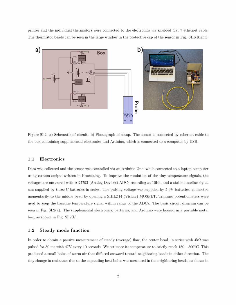
Figure SI.2: a) Schematic of circuit. b) Photograph of setup. The sensor is connected by ethernet cable to

the box containing supplemental electronics and Arduino, which is connected to a computer by USB.

1.1 Electronics

Data was collected and the sensor was controlled via an Arduino Uno, while connected to a laptop computer

using custom scripts written in Processing. To improve the resolution of the tiny temperature signals, the

voltages are measured with AD7793 (Analog Devices) ADCs recording at 10Hz, and a stable baseline signal

was supplied by three C batteries in series. The pulsing voltage was supplied by 5 9V batteries, connected

momentarily to the middle bead by opening a SIHLZ14 (Vishay) MOSFET. Trimmer potentiometers were

used to keep the baseline temperature signal within range of the ADCs. The basic circuit diagram can be

seen in Fig. SI.2(a). The supplemental electronics, batteries, and Arduino were housed in a portable metal

box, as shown in Fig. SI.2(b).

1.2 Steady mode function

In order to obtain a passive measurement of steady (average) flow, the center bead, in series with 4kΩ was

pulsed for 30 ms with 47V every 10 seconds. We estimate its temperature to briefly reach 180 − 300C. This

produced a small bolus of warm air that diffused outward toward neighboring beads in either direction. The

tiny change in resistance due to the expanding heat bolus was measured in the neighboring beads, as shown in

2

0 2 4 6 8 10Time(seconds)

5000

0

5000

10000

15000

20000

25000

30000

Rea

ding

Upper BeadLower Bead

0 2 4 6 8 10Time(seconds)

5000

0

5000

10000

15000

20000

25000

30000

Rea

ding

Upper BeadLower Bead

0 2 4 6 8 10Time(seconds)

5000

0

5000

10000

15000

20000

25000

30000R

eadi

ng

Upper BeadLower Bead

0 2 4 6 8 10Time(seconds)

5000

0

5000

10000

15000

20000

25000

30000

Rea

ding

Upper BeadLower Bead

h1

h2

0 2 4 6 8 10 12Time(seconds)

5000

0

5000

10000

15000

20000

Rea

ding

Upper BeadLower Bead

d)b)

a)

0 2 4 6 8 10 12Time(seconds)

5000

0

5000

10000

15000

20000

Rea

ding

Upper BeadLower Bead

0 2 4 6 8 10 12Time(seconds)

5000

0

5000

10000

15000

20000

Rea

ding

Upper BeadLower Bead

0 2 4 6 8 10 12Time(seconds)

5000

0

5000

10000

15000

20000

Rea

ding

Upper BeadLower Bead

h1

h2

c)

Time(seconds) Time(seconds)

Reading

Reading

Figure SI.3: Averaged responses from two thermistors as heat bolus diffuses away from center bead for a)

Zero flow b) 1.6 cm/s downwards flow in calibration tube. c, d) Averaged responses before subtraction of

temperature drift. Probe was intentionally heated before placement in tube for explanatory purposes.

Fig. SI.3. In the absence of flow through the sensor, there is a slight upward bias in the response magnitudes

due to thermal buoyancy of the bolus. Upward and downward flow biases the relative responses of the two

thermistors in a reproducible way. The log of the ratio of the maxima ln(h1/h2) was used as a metric to

calculate flow velocity (see steady flow calibration section). For experimental data sets, temperature drift

must be subtracted as the probe equilibrates with the interior flute temperature.

1.3 Transient mode function

While in steady mode, infrequent, brief pulsing of heat avoids troublesome induced convective currents, it

prohibits measurement of high frequency(& .1 Hz) changes in flow. In transient mode of the same sensor,

continuous voltage 47 V is applied across the middle bead, such that transients in the flows can be measured

from the instantaneous ratio of responses in the neighboring beads. The trade-off is that information about

the baseline flow is lost, because induced currents, which depend on several parameters, including unknown

details of tunnel geometry, can dominate the signal. Fig. SI.4 shows the response of the neighboring beads

in transient mode for some prescribed transients. At ∼ 0 cm/s the dependence on the difference between

the two readings is the weakest(∼ 30,000cm/s ); assuming that slope, the largest fluctuation observed in the field

3

0 100 200 300 400 500 600 700Time(seconds)

−200000

−150000

−100000

−50000

0

50000

100000

150000

Rea

ding

Upper BeadLower Bead

0 1 2 3 4 5 6 7 0 -1 -2 -3 -4 -5 -6 -7 0Velocity(cm/s .64)·

Figure SI.4: Relative readings upper and lower beads in transient mode as flow was varied in increments of

.64cm/s

corresponded to ∼ 1mm/s.

1.4 Steady flow calibration

A 5.6 cm diameter, 2m long, vertical acrylic tube was used as a sample conduit for calibration of the sensor

(see Fig. SI.5). The tube was covered with a layer of thermal insulation to prevent external thermal gradients

from influencing flow, which was observed when the bottom of the tube was exposed to the sun through a lab

window. Air was pulled through the tube by a vacuum source and mass flow controller (Alicat MC-20slpm)

in series. To prevent heterogeneous inertial flows where the narrow connector tube met the wider conduit,

air was directed through a fine metal mesh before entering a conical flow rectifier. The whole set-up was

up-down symmetric, such that by rotating two valves, flow direction could be reversed without changing the

setup geometry. The sensor was inserted into a hole in the middle of the tube and oriented so that the beads

were aligned with the tube.

As a consistency check and to eliminate possible systematic biases in the probe, every airflow measurement

is taken twice using the same probe in two orientations. In one the (arbitrarily named) first bead is above

the middle thermistor(’upward’); in the other it is directly below (’downward’). To do so, we need separate

calibration tables for the ’upward’ and ’downward’ orientations.

Fig. SI.6 shows the dependence of the metric on flow velocity in the calibration tube. The typical

standard deviation between pulses during calibration is small and does not represent the dominant source

of error in the field, where variation in conduit geometry plays a larger role (see Experimental Procedure).

4

Figure SI.5: Schematic of tube used for calibration. Arrows show direction path of air from inlet toward

vacuum source.

There is an unusual, though robust, feature at ∼ ±2cm/s, where the response briefly jumps. This is most

likely an effect due to shifting from a regime of viscously dominated laminar flow to inertial dominated

laminar flow. We note that this leads to a small range of flow velocities where we overestimate the flow

speed(but not the sign).

Fig. SI.7 shows several calibration curves for the different instances of the sensor, either a spare duplicate

sensor, or the same physical sensor after thermistor beads were replaced. Each instance requires a new

calibration, as the the magnitudes of bead responses varies according to the manufacturer’s 25% tolerance,

but upon shifting the vertical offset and slope, on can see the qualitative behavior of each instance is the

same.

1.5 Temperature and humidity dependence

While the calibration curve in laboratory conditions is robust, additional tests were performed to make sure

that our metric was not terribly sensitive to other factors which can vary in the field. Two such factors

which should influence the thermal response of the sensor, and therefore its performance are background

temperature and humidity. Fig. SI.8 shows the calibration curve for two different ambient temperatures,

which roughly represent the range of temperature in the mound. Though the curve has a lower slope at

5

−3 −2 −1 0 1 2 3

Velocity(cm/s)

−1.0

−0.5

0.0

0.5

1.0

1.5

Met

ric

−3 −2 −1 0 1 2 3Velocity(cm/s)

−1.0

−0.8

−0.6

−0.4

−0.2

0.0

0.2

0.4

0.6

0.8

Met

ric

UpwardsDownwards

Upwards ProbeDownwards Probe

−3 −2 −1 0 1 2 3Velocity(cm/s)

−1.0

−0.8

−0.6

−0.4

−0.2

0.0

0.2

0.4

0.6

0.8

Metric

UpwardsDownwards

Met

ric

(ln(h

1/h

2))

Velocity (cm/s)

Figure SI.6: Calibration curves for steady flow sensor measured in the plastic tube. The upwards black

triangles represent the upwards orientation of the sensor, while the downwards blue triangles represent the

downwards orientation. Error bars are the pulse-to-pulse deviation.

higher temperature, which indicates that the sensor underestimates hotter flows, this effect is small compared

to the variation of the daily mound flow schedule measured in the field, and would not account for the sign

change. The metric, continuously measured for constant flow was unaffected by a change in ambient relative

humidity from 25% to 70% (at 29C).

We can estimate this effect by applying a temperature-dependent calibration, where sensitivity is assumed

to vary linearly with temperature, interpolated between the slope and offset of the 21 and 29 curves. Using

this with the temperature information from inside the mound, the effect of temperature on all live mound

values can be approximated, as shown in Fig. SI.9. We can see the values are only slightly modified, causing

a tiny enhancement to the trend, where daytime flows become slightly more positive.

1.6 Orientational Dependence

As mentioned above, the sensor is calibrated exclusively for vertical flow. Though it was not difficult to

ensure that local conduit orientation was vertical where the sensor was placed, and that flow was there-

fore predominantly vertical, it is not unreasonable to suspect that a horizontal flow component could be

misinterpreted by the sensor.

6

−4 −2 0 2 4

Velocity(cm/s)

−1.5

−1.0

−0.5

0.0

0.5

1.0

1.5

Met

ric

Upwards ProbeDownwards Probe

−3 −2 −1 0 1 2 3Velocity(cm/s)

−1.0

−0.8

−0.6

−0.4

−0.2

0.0

0.2

0.4

0.6

0.8

Met

ric

UpwardsDownwards

−3 −2 −1 0 1 2 3Velocity(cm/s)

−1.0

−0.8

−0.6

−0.4

−0.2

0.0

0.2

0.4

0.6

0.8

Met

ric

UpwardsDownwards

−3 −2 −1 0 1 2 3Velocity(cm/s)

−1.0

−0.8

−0.6

−0.4

−0.2

0.0

0.2

0.4

0.6

0.8

Met

ric

UpwardsDownwards

−3 −2 −1 0 1 2 3Velocity(cm/s)

−1.0

−0.8

−0.6

−0.4

−0.2

0.0

0.2

0.4

0.6

0.8

Metric

UpwardsDownwards

−3 −2 −1 0 1 2 3Velocity(cm/s)

−1.0

−0.8

−0.6

−0.4

−0.2

0.0

0.2

0.4

0.6

0.8

Metric

UpwardsDownwards

−3 −2 −1 0 1 2 3Velocity(cm/s)

−1.0

−0.8

−0.6

−0.4

−0.2

0.0

0.2

0.4

0.6

0.8

Metric

UpwardsDownwards

Met

ric

(ln(h

1/h

2))

Velocity (cm/s)

Figure SI.7: Shifted calibration curves for three instances of the sensor reveal a predictable relationship

between metric and velocity.

Fig. SI.10 shows the metric as a function of flow velocity for 3 orientations of the calibration tube;

horizontal, 45, and vertical, when the sensor is either parallel or orthogonal (cap windows 90 from tube

axis). Negligible change in metric for all orientations in which the sensor was misaligned indicates that the

sensor cap effectively rectifies flow for all orientations; any flow component perpendicular to the sensor would

have negligible effect on the measured value. When the flow is aligned with the sensor, for the full range of

probe and tube orientations, there is only a small shift in the curve. Additionally, Fig. SI.11 shows that a

vertically placed sensor’s sensitivity to flow decreases to zero as the direction of flow is changed from vertical

to horizontal. These rule out the possibility of non-trivial sensitivity to conduit orientation.

Fig. SI.12 shows the metric as a function of probe angle in a vertical tube of constant flow velocity 3.1

cm/s, where the probe is aligned (0) or orthogonal (±90) to the tube. The good fit to a cosine shows that

flows not aligned with the probe (horizontal flows in the field) do not significantly affect the measurement.

7

−1.0 −0.5 0.0 0.5 1.0

Velocity(cm/s)

0.2

0.3

0.4

0.5

0.6

0.7

Met

ric

−1.5 −1.0 −0.5 0.0 0.5 1.0 1.5Velocity(cm/s)

0.2

0.3

0.4

0.5

0.6

0.7

Met

ric

21C29C

Met

ric

(ln(h

1/h

2))

Velocity (cm/s)

Figure SI.8: Calibration curves for two temperatures show a slight shift(∼ 0.2cm/s) and slope change

(∼ 40%) for this temperature difference, which is closely matched with the total range observed in live

mounds. Horizontal and vertical lines are to guide the eye.

2 Additional Measurements: Long-term flow in a dead mound

Continuous flow in five flutes from the dead mound were measured, shown in Fig. SI.13. Four out of five

flutes follow the observed trend. The heterogeneity is likely due to the complex geometry and is consistent

with the few live mound measurements which also go against the trend.

One flute (which happened to go against the observed trend) was measured for three days. For the

first two days, the mound (at the edge of a forest) was exposed to partial direct sunlight. It can be seen

in Fig. SI.15 that the measured air velocity strictly follows a daily schedule, where fine features repeat

themselves. On the third day, a tarp was positioned above the mound, keeping the mound shaded from any

direct sunlight, but exposed to ambient temperatures. Some midday features are missing, presumably those

directly induced by solar heating, but the general trend remains the same.

3 Permeability Measurements

The mound material is 37−47% air by volume, and has an average pore size of ∼ 5µm, roughly the mean

8

−6

−3

0

3

6

Air

Velo

city

(cm

/s)

−6

−3

0

3

6A

irVe

loci

ty(c

m/s

)

0 6 12 18 24

Hour of day

0

1

2

3

4

5

6

CO

2(%

)

NestChimney

−6

−3

0

3

6

∆T

(C

)

Flow∆T

−6

−3

0

3

6

∆T

(C

)

Flow∆T

No Thermal Correction

−6

−3

0

3

6A

irVe

loci

ty(c

m/s

)

−6

−3

0

3

6

Air

Velo

city

(cm

/s)

0 6 12 18 24

Hour of day

0

1

2

3

4

5

6

CO

2(%

)

NestChimney

−6

−3

0

3

6

∆T

(C

)

Flow∆T

−6

−3

0

3

6

∆T

(C

)

Flow∆T

With Thermal Correction−6

−3

0

3

6A

irVe

loci

ty(c

m/s

)

−6

−3

0

3

6

Air

Velo

city

(cm

/s)

0 6 12 18 24

Hour of day

0

1

2

3

4

5

6

CO

2(%

)

NestChimney

−6

−3

0

3

6

∆T

(C

)

Flow∆T

−6

−3

0

3

6

∆T

(C

)

Flow∆TFigure SI.9: Comparison of calculated velocities where temperature-dependent sensitivity is taken into ac-

count

.

−3 −2 −1 0 1 2 3Velocity(cm/s)

−1.0

−0.8

−0.6

−0.4

−0.2

0.0

0.2

0.4

0.6

0.8

Met

ric

−3 −2 −1 0 1 2 3Velocity(cm/s)

−1.0

−0.8

−0.6

−0.4

−0.2

0.0

0.2

0.4

0.6

0.8

Met

ric

UpwardsDownwards

−3 −2 −1 0 1 2 3Velocity(cm/s)

−1.0

−0.8

−0.6

−0.4

−0.2

0.0

0.2

0.4

0.6

0.8

Met

ric

UpwardsDownwards

−3 −2 −1 0 1 2 3Velocity(cm/s)

−1.0

−0.8

−0.6

−0.4

−0.2

0.0

0.2

0.4

0.6

0.8

Met

ric

UpwardsDownwards

−3

−2

−1

01

23

Velocity(cm/s)

−1.0

−0.8

−0.6

−0.4

−0.2

0.0

0.2

0.4

0.6

0.8

Metric

Upw

ardsD

ownw

ards

−3

−2

−1

01

23

Velocity(cm/s)

−1.0

−0.8

−0.6

−0.4

−0.2

0.0

0.2

0.4

0.6

0.8

Metric

Upw

ardsD

ownw

ards

−3

−2

−1

01

23

Velocity(cm/s)

−1.0

−0.8

−0.6

−0.4

−0.2

0.0

0.2

0.4

0.6

0.8

Metric

Upw

ardsD

ownw

ards

ParallelOrthogonal

Met

ric

(ln(h

1/h

2))

Velocity (cm/s)

Figure SI.10: Velocity metric as a function of flow speed tube orientation and relative probe orientation.

Regardless of whether the tube is vertical (red), diagonal (45, black) or horizontal (blue), the probe is only

sensitive to flow velocity when the probe is aligned parallel with the tube (upwards triangles), and not when

orthogonal (rightwards triangles)

particle size [2]. To determine the degree to which this admits bulk flow of air, air was pulled through the

tube by a vacuum source, mass flow controller (Alicat MC-20slpm), and conical sample of mound wall sealed

9

−3 −2 −1 0 1 2 3Velocity(cm/s)

−0.8

−0.6

−0.4

−0.2

0.0

0.2

0.4

0.6

0.8

Met

ric

−3 −2 −1 0 1 2 3Velocity(cm/s)

−0.8

−0.6

−0.4

−0.2

0.0

0.2

0.4

0.6

0.8

Met

ric

−3 −2 −1 0 1 2 3Velocity(cm/s)

−0.8

−0.6

−0.4

−0.2

0.0

0.2

0.4

0.6

0.8

Met

ric

−3 −2 −1 0 1 2 3Velocity(cm/s)

−0.8

−0.6

−0.4

−0.2

0.0

0.2

0.4

0.6

0.8

Met

ric

Vertical TubeDiagonal TubeHorizontal Tube

Met

ric

(ln(h

1/h

2))

Velocity (cm/s)

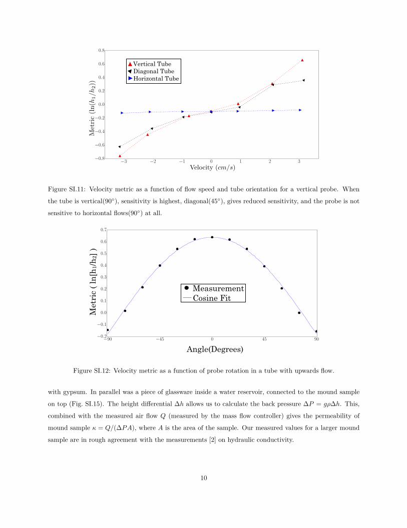
Figure SI.11: Velocity metric as a function of flow speed and tube orientation for a vertical probe. When

the tube is vertical(90), sensitivity is highest, diagonal(45), gives reduced sensitivity, and the probe is not

sensitive to horizontal flows(90) at all.

−90 −45 0 45 90Angle(Degrees)

−0.2

−0.1

0.0

0.1

0.2

0.3

0.4

0.5

0.6

0.7

Met

ric

Angle(Degrees)

Measurement Cosine Fit

−90 −45 0 45 90Angle(Degrees)

−0.2

−0.1

0.0

0.1

0.2

0.3

0.4

0.5

0.6

0.7

Met

ric

Met

ric

( ln

[h1/

h2]

)

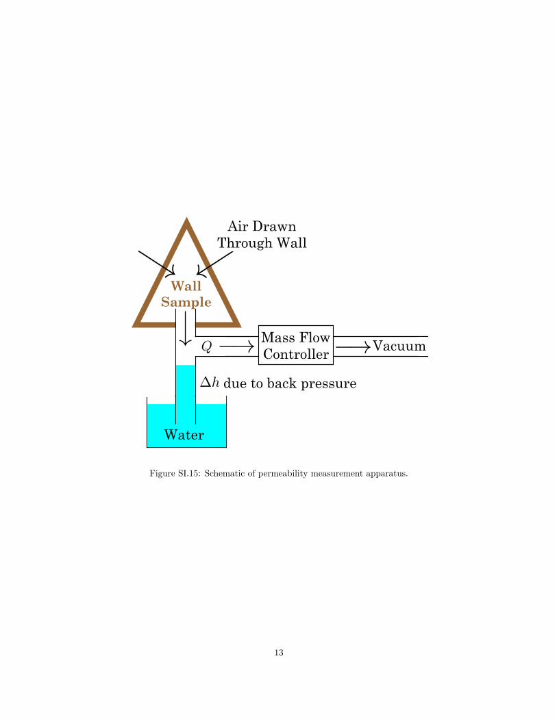
Figure SI.12: Velocity metric as a function of probe rotation in a tube with upwards flow.

with gypsum. In parallel was a piece of glassware inside a water reservoir, connected to the mound sample

on top (Fig. SI.15). The height differential ∆h allows us to calculate the back pressure ∆P = gρ∆h. This,

combined with the measured air flow Q (measured by the mass flow controller) gives the permeability of

mound sample κ = Q/(∆PA), where A is the area of the sample. Our measured values for a larger mound

sample are in rough agreement with the measurements [2] on hydraulic conductivity.

10

0 3 6 9 12 15 18 21 24

Hour of day

−6

−4

−2

0

2

4

6

Air

Velo

city

(cm

/s)

0 3 6 9 12 15 18 21 24

Hour of day

−6

−4

−2

0

2

4

6

Air

Velo

city

(cm

/s)

0 3 6 9 12 15 18 21 24

Hour of day

−6

−4

−2

0

2

4

6

Air

Velo

city

(cm

/s)

Figure SI.13: Continuous flow measurements of 5 flutes in a dead mound.

References

[1] Olson DE, Parker KH, Snyder B (1984) A pulsed wire probe for the measurement of velocity and flow

direction in slowly moving air. J Biomech Eng 106:72–8.

[2] Kandasami R, Borges R, Murthy T (2015) in preparation.

11

0 6 12 18 24Hour of Day

0.0

0.2

0.4

0.6

0.8

1.0

1.2

1.4

1.6

1.8

Velo

city

(cm

/s)

Day 1Day 2Day 3

0 6 12 18 0 6 12 18 0 6 12 18 0Hour of Day

0.0

0.2

0.4

0.6

0.8

1.0

1.2

1.4

1.6

1.8

Velo

city

(cm

/s)

Tarp . . . . . . . . . . . . . .a)

b)

Figure SI.14: a) 3 day flute flow measurement. A tarp was hung to shade the mound on the third day. b)

The same data, with days 1, 2, 3 overlaid on top of each other.

12

−→

−→−→

−→−→Q

Mass Flow Controller

Vaccuum

Vacuum

Wall Sample

Air Drawn Through Wall

∆h due to back pressure

Water

Figure SI.15: Schematic of permeability measurement apparatus.

13