Terminus-driven retreat of a major southwest Greenland ...

Terminus-driven retreat of a major southwest Greenland tidewaterglacier during the early 19th century: insights from glacier

reconstructions and numerical modelling

James M. LEA,1 Douglas W.F. MAIR,1 Faezeh M. NICK,2,3 Brice R. REA,1

Anker WEIDICK,4 Kurt H. KJÆR,5 Mathieu MORLIGHEM,6 Dirk VAN AS,4

J. Edward SCHOFIELD1

1Department of Geography and the Environment, University of Aberdeen, Aberdeen, UKE-mail: [email protected]

2The University Centre in Svalbard (UNIS), Longyearbyen, Norway3Centre for Ice and Climate, Niels Bohr Institute, University of Copenhagen, Copenhagen, Denmark

4Geological Survey of Denmark and Greenland (GEUS), Copenhagen, Denmark5Centre for GeoGenetics, Natural History Museum of Denmark, University of Copenhagen, Copenhagen, Denmark

6Department of Earth System Science, University of California, Irvine, Irvine, CA, USA

ABSTRACT. Tidewater glaciers in Greenland experienced widespread retreat during the last century.

Information on their behaviour prior to this is often poorly constrained due to lack of observations,

while determining the drivers prior to instrumental records is also problematic. Here we present a

record of the dynamics of Kangiata Nunaata Sermia (KNS), southwest Greenland, from its Little Ice Age

maximum (LIAmax) to 1859 – the period before continuous air temperature observations began at Nuuk

in 1866. Using glacial geomorphology, historical accounts, photographs and GIS analyses, we provide

evidence KNS was at its LIAmax by 1761, had retreated by �5 km by 1808 and a further 7 km by 1859.

This predates retreat at Jakobshavn Isbræ by 43–113 years, demonstrating the asynchroneity of

tidewater glacier terminus response following the LIA. We use a one-dimensional flowband model to

determine the relative sensitivity of KNS to atmospheric and oceanic climate forcing. Results

demonstrate that terminus forcing rather than surface mass balance drove the retreat. Modelled glacier

sensitivity to submarine melt rates is also insufficient to explain the retreat observed. However,

moderate increases in crevasse water depth, driving an increase in calving, are capable of causing

terminus retreat of the observed magnitude and timing.

KEYWORDS: glacial geomorphology, glacier calving, glacier fluctuations, glacier modelling

INTRODUCTION

Tidewater glaciers (TWGs) exert a major control on theshort- and long-term mass balance of the Greenland icesheet (Van den Broeke and others, 2009; Alley and others,2010; Bevan and others, 2012). The availability of satellitedata has allowed their dynamics to be documented in detailover the past two decades (Moon and Joughin, 2008; Boxand Decker, 2011; Moon and others, 2012). Prior to this,TWG dynamics are poorly constrained by observations,placing limitations on the knowledge of their response toclimate change. Multi-decadal records of terminus fluctua-tions are available for some TWGs back to the 1930s, andlimited direct observations exist before this (Bjørk andothers, 2012). There is limited potential to extend TWGrecords to their Little Ice Age maxima (LIAmax) due to thesparse and often indirect nature of observations (Weidick,1959, 1968; Briner and others, 2010; Larsen and others,2011). Characterization of TWG behaviour during the 18thand 19th centuries is therefore problematic. However,where this is possible it provides insights into centennial-timescale TWG behaviour, and important context for con-temporary observations and potential TWG response tofuture climate forcing.

Predicting the response of the Greenland ice sheet (GrIS)to climate change is dependent on understanding how TWGprocesses and behaviour are affected by climatic forcings

(Van den Broeke and others, 2009; Rignot and others, 2010).Although TWG stability is thought to be controlled by acombination of atmospheric and oceanic forcings occurringat the terminus, the precise processes and their relativeimportance are still poorly understood (Holland and others,2008; Nick and others, 2009; Murray and others, 2010;Rignot and others, 2010, 2012; Straneo and others, 2010,2012). Modelling of the GrIS is limited further by the shortobservation periods of dynamics available for calibrationand validation, model computational requirements andresolution, and availability of detailed bed topography (Vieliand Nick, 2011). These can be mitigated by employingspatially reduced models to evaluate glacier catchment-scale responses to different forcings (Thomas, 2004; Nickand others, 2009, 2010, 2012, 2013; Joughin and others,2010a; Colgan and others, 2012). Application of thesemodels where TWG records can be extended to theirLIAmax allows the potential drivers of post-LIAmax GrISretreat to be investigated.

The earliest post-LIAmax TWG retreats in Greenland areknown to have occurred prior to the first continuous airtemperature record at Nuuk in 1866 (Weidick, 1959, 1968;Vinther and others, 2006; Weidick and others, 2012). Thiscan preclude direct comparison of post-LIAmax TWGresponse to climate, including the first observed retreat ofJakobshavn Isbræ between 1851 and 1875 (Weidick and

Journal of Glaciology, Vol. 60, No. 220, 2014 doi: 10.3189/2014JoG13J163 333

Bennike, 2007; Csatho and others, 2008). Application ofcatchment-scale models where climate data are lackingallows the drivers of individual TWG change to be investi-gated through series of model sensitivity experiments. Thesefacilitate comparisons of modelled behaviour to observa-tions, and can be used to identify the range of forcings andlikely mechanism(s) required to explain the observed retreat.

This study investigates the post-LIAmax dynamics ofKangiata Nunaata Sermia (KNS), southwest Greenland, priorto the instrumental air temperature record. We aim toimprove the record of post-LIAmax fluctuations of KNS usingpreviously unstudied geomorphology, newly uncoveredhistorical sources, geospatial analyses, and previouslypublished lines of evidence (Weidick, 1959; Weidick andothers, 2012). Secondly, we evaluate whether the post-LIAmax retreat is best explained by changes in surface massbalance (SMB) or forcing perturbations occurring at theterminus. This is achieved using a one-dimensional (1-D)flowband numerical model (Nick and others, 2010).

FIELD SITE

KNS is located �100 km from Nuuk at the head of theKangersuneq branch of Godthabsfjord, southwest Green-land (Fig. 1). The terminus retreated significantly during the19th century, though uncertainty exists regarding the timingand scale of this retreat (Weidick, 1959; Weidick and others,2012). The glacier catchment is �31 400 km2, and has acontemporary calving flux in excess of 6 km3 a–1, making itthe largest outlet glacier in western Greenland located southof Jakobshavn Isbræ (Van As and others, 2014). At itsLIAmax, KNS was advanced >22 km further down-fjord of its

current terminus position, occupying a topographic depres-sion on the west side of the fjord, and forming a large ice-dammed lake (IDL) in the forefield of Qamanarssup Sermia(QS; Weidick and others, 2012).

Subsurface West Greenland Current (WGC) waters peri-odically enter Godthabsfjord over a shallow (80m) sill at theentrance to the fjord, establishing a link between the oceanand the terminus (Mortensen and others, 2011, 2013). Fjordcirculation allows surface heated waters to mix downwardto subsurface fjord waters, which can also interact with theterminus (Mortensen and others, 2011). No direct measure-ments of submarine melt (SM) exist for KNS, althoughestimates of SM at vertical calving fronts of other WestGreenland TWGs range from 0.7�0.2 to 3.9�0.8md–1

(Rignot and others, 2012). Within this range, SM for KNS isprobably at the lower end due to the sill at the fjord entrancelimiting the ability of warm WGC waters to reach theterminus (Straneo and others, 2012).

METHODS FOR RECONSTRUCTING AND DATINGGLACIER TERMINUS POSITIONS

The LIAmax extent of KNS is clearly defined by a series ofmoraines and ice-scour limits (Weidick and Citterio, 2011;Weidick and others, 2012). These limits and the geo-morphology inside were mapped in detail using high-resolution (2m2) GeoEye satellite imagery, and ground-truthed during fieldwork conducted in 2011. Reconstruc-tions of glacier geometry were obtained by extractingelevations of mapped moraine limits from an aerophoto-grammetrically derived digital elevation model (DEM) of theKNS terminus area, based on a 1985 aerial survey

Fig. 1. Hillshaded digital elevation model (photogrammetric DEM and ASTER GDEM mosaic), showing the post-LIAmax geomorphology,and the possible terminus positions/ranges relative to the 2012 terminus position. The 2012 terminus position was mapped from a Landsatimage acquired on 18 September 2012. Minimum extent for 1859 position is taken from 1946 terminus position, observed prior todisintegration of the confluence by 1948 (Weidick and Citterio, 2011). Inset is a panchromatic Landsat image of the Godthabsfjord regionacquired on 19 September 1992.

Lea and others: Greenland tidewater glacier retreat during the 19th century334

conducted by the Danish Geodata Agency with associatedground control (GR96) and error of �6m. Where coveragefrom this DEM was unavailable, Advanced SpaceborneThermal Emission and Reflection Radiometer (ASTER) globalDEM (GDEM) data (http://asterweb.jpl.nasa.gov/gdem.asp)gridded to 30m2 resolution were used (Fig. 1). Moraineelevations were extracted relative to the glacier/fjord centreline (also used as the model flowline) using the extrapolatedcentre-line method presented in Lea and others (2014). Thisallowed moraine elevation profiles to be directly andaccurately compared to the modelled glacier elevationprofiles (e.g. Fig. 9, further below).

The date and location of terminus positions werereconstructed using an array of historical sources, whichare discussed in detail below. The physical plausibility ofeach account was tested where possible, to establish thelevel of confidence that could be placed in each obser-vation. In some cases, GIS tools could be applied toconstrain terminus locations with greater absolute precisionthan allowed by qualitative analysis alone.

Historical accounts

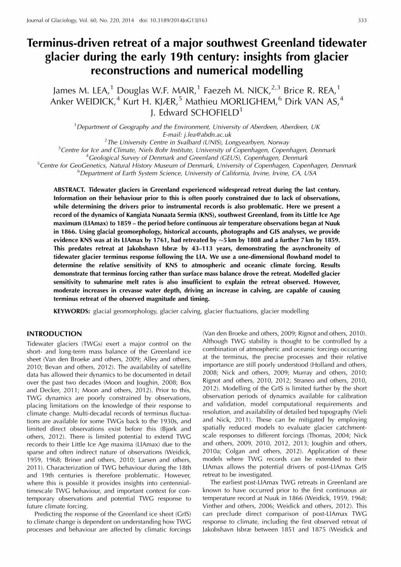
The earliest terminus position of KNS that can be determinedis from the observations of David Crantz in 1761 (publishedin English in 1820). He describes observing an unnamedglacier in Baal’s Rivier (a previous name for Godthabsfjordand Kangersuneq) that ‘ascends in steps for the space of fourleagues [�22 km]’, while ‘[a] low hill ... closed the vista’,and ‘large tracts of ice ... branched off north and south to anunknown distance into the country’ (Crantz, 1820, p. 34).Crantz’s viewpoint has been reconstructed to be from thevalley separating Kangersuneq and Amitsuarssuk fjordbranches (Fig. 2). This is based on his account of hisapproach to the observation point, describing hiking along avalley through which flowed a ‘rivulet, swelling at intervalsinto pools’, and with Norse ruins located adjacent to ‘a greatlake of freshwater’ (Crantz, 1820, p. 33). The valleyidentified is the only one in the region that fits Crantz’sdescription (Fig. 2a). KNS is also the only observable TWGfrom this viewpoint, with Nunatarssuk likely to be the lowhill mentioned, located 20 km from LIAmax (Fig. 2b).

The next reference to KNS is from Egil Thorhallesen, who,guided by locals, visited an IDL between 1765 and 1775previously identified as Isvand (Fig. 2; Weidick, 1959;Weidick and others, 2012). The account does not relate adirect observation of the terminus, though it is of potentialrelevance since the ice margin position at Isvand wasdynamically linked to the terminus retreat of KNS during the20th century (Weidick and Citterio, 2011). The wording ofThorhallesen’s account is ambiguous in that it reports that‘the glacier has laid itself in recent time’ over Isvand(Thorhallesen, 1776, p. 37). This makes it unclear whetherhe is referring to a recent advance or retreat of the ice marginfrom its observed position.

The diaries of Karl Ludwig Giesecke record a visit made tothe terminus area of KNS in August 1808 (published inGerman in 1910). He describes the ice having nearlyoverridden the Norse ruins indicated in Figure 1 at itsmaximum extent, though the retreated terminus is stillnearby. He makes a comparative assessment of the glaciergeometry as being ‘grosser, steiler, und gefahrlicher als derNordostliche’ (larger, steeper and more dangerous than thatto the north-east [Qamanarssap Sermia]; trans. by N. Weitz)(Giesecke, 1910, p. 151), and describes an IDL occupying theQS forefield which ‘uber die Felsenwand hinab am Eisblinkins Meer sturzt’ (next to the glacier flows over a rock wall intothe ocean; trans. by N. Weitz) (Giesecke, 1910, p. 151).

Maps and photographic evidence

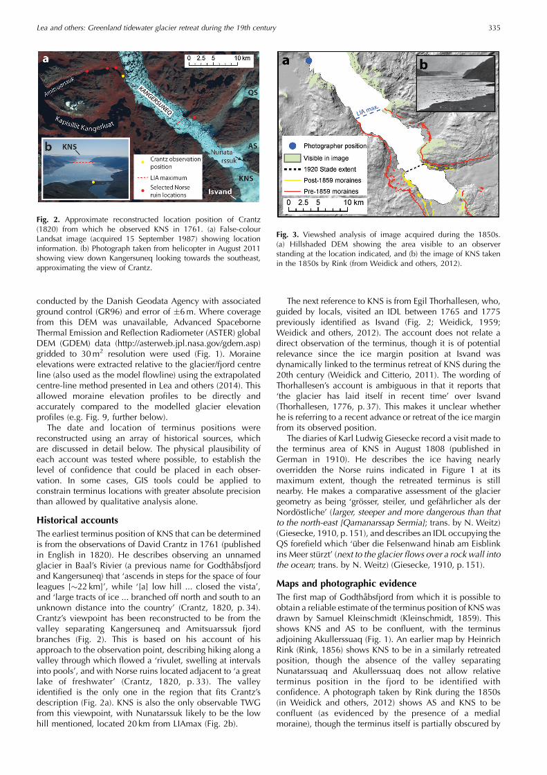
The first map of Godthabsfjord from which it is possible toobtain a reliable estimate of the terminus position of KNS wasdrawn by Samuel Kleinschmidt (Kleinschmidt, 1859). Thisshows KNS and AS to be confluent, with the terminusadjoining Akullerssuaq (Fig. 1). An earlier map by HeinrichRink (Rink, 1856) shows KNS to be in a similarly retreatedposition, though the absence of the valley separatingNunatarssuaq and Akullerssuaq does not allow relativeterminus position in the fjord to be identified withconfidence. A photograph taken by Rink during the 1850s(in Weidick and others, 2012) shows AS and KNS to beconfluent (as evidenced by the presence of a medialmoraine), though the terminus itself is partially obscured by

Fig. 2. Approximate reconstructed location position of Crantz(1820) from which he observed KNS in 1761. (a) False-colourLandsat image (acquired 15 September 1987) showing locationinformation. (b) Photograph taken from helicopter in August 2011showing view down Kangersuneq looking towards the southeast,approximating the view of Crantz.

Fig. 3. Viewshed analysis of image acquired during the 1850s.(a) Hillshaded DEM showing the area visible to an observerstanding at the location indicated, and (b) the image of KNS takenin the 1850s by Rink (from Weidick and others, 2012).

Lea and others: Greenland tidewater glacier retreat during the 19th century 335

foreground topography (Fig. 3b). This prevents the identifi-cation of the exact position of the terminus from this image.

RESULTS

Post-LIAmax geomorphology

Figure 1 shows the post-LIAmax geomorphology of KNS. Allsubsequent mentions of glacier terminus positions are givenrelative to the 2012 terminus, indicated by the fjord centreline (Fig. 1). The maximum moraine/ice-scour extent is22.6 km, and covers an area 220 km2 greater than at present.Multiple sets of moraines exist on both flanks of the fjordwithin the LIAmax. These include:

An upper set of well-developed continuous lateralmoraines/ice scour on both sides of the fjord delimitingthe LIAmax. On the eastern fjord flank the moraine spansthe forefield area of the land-terminating glacier Qama-narssup Sermia (QS), while the moraine on the westernflank extends inland into the topographic depressionopposite Akullerssuaq (Fig. 1).

Several other less pronounced moraines lie proximal andsub-parallel to well-developed upper moraines in the QSforefield on the eastern flank, and also within thetopographic depression opposite Akullerssuaq onthe western flank. Fluted moraines occupy areas withinthe LIAmax extent of the QS forefield and between theLIAmax and 1920 Stade moraines on the western flank.These are broadly orientated according to the slope oflocal topography (Fig. 1).

A lower set of moraines/ice scour extends to �10 kmalong both sides of the fjord. On the eastern flank thiswraps around Akullerssuaq, and on the less steepwestern flank several inset sub-parallel moraines arepresent. The outer limit of these has previously beenrelated to the culmination of the 1920 Stade readvance(Weidick and Citterio, 2011).

Trimline elevations show that glacier surface elevation from�20 km to the LIAmax extent did not exceed 100ma.s.l.,

with an average surface gradient of 1.68 (Fig. 4). The glaciersurface significantly steepens upstream between 20 and18 km to 4.28, before surface elevation appears to decreasewhere the QS forefield adjoins Kangersuneq between 14and 18 km (Fig. 4). The ice surface steepens to 3.68 as thefjord narrows between 12 and 14 km, before levelling outbetween 10 and 12 km opposite Akullerssuaq as the iceextends into the topographic depression (Figs 1 and 4). Theice surface rises by �200m between 2 and 10 km (1.48surface slope), with the gradient doubling to 2.88 between1 and 2 km, reaching an elevation of �600ma.s.l. This finalelevation step change occurs immediately upstream of theconfluence with AS (Fig. 4).

Reconstructing timing of terminus fluctuations:LIAmax–1859

The account of Crantz describing KNS extending fromNunatarssuk for �20 km corresponds almost exactly withthe LIAmax extent of the glacier (Figs 2 and 3). Hisdescription of the glacier profile as ‘ascending in steps’(1820, p. 34) also fits with the reconstructed LIAmaxgeometry of KNS, with at least three changes in surfacegradient identified (Fig. 4). It is proposed that Crantzobserved KNS at or very near its LIAmax extent in 1761.

Giesecke’s (1910) description of an IDL draining directlyover land into the fjord provides excellent constraint on theterminus position in 1808. For this drainage to occur, theeastern margin of KNS must be sufficiently retreated fromLIAmax to allow the IDL to drain into the fjord over land,rather than subglacially or as an ice-marginal channel. Toestablish the terminus configurations where it is physicallypossible to maintain an IDL in the QS forefield, which alsodrains into the fjord over land, an analysis of possible lakedrainage pathways was conducted using the ArcHydro add-on to ArcMap v.10 software. Using the DEM shown inFigure 1, dams were inserted along the LIAmax morainesspanning the QS forefield, allowing the IDL and its drainagepaths to be reconstructed. Four possible land drainage pathscould maintain the IDL, located within a terminus range of�550m (Fig. 1). However, since the majority of this range iswithin a section of the fjord that begins to widen, from aglaciological perspective the narrower section of the fjordrepresents a more likely location for the terminus (Mercer,1961). The 1808 terminus location on the western flank isless certain, though a likely range of terminus configurationsis indicated in Figure 1.

The smaller, less continuous inset moraines subparallel tothe LIAmax suggest glacier thinning from the LIAmax. Thesteep fjord valley side topography that extends between17 and 22 km provides low preservation potential formoraines, meaning that the style of retreat from 1761 to1808 cannot be reconstructed with confidence.

Map evidence places the terminus of KNS as adjoiningAkullerssuaq in 1859 (Kleinschmidt, 1859). Viewshed analy-sis applied to the photograph taken by Rink in the 1850s(Rink, 1856) allows the maximum possible extent of theterminus to be reconstructed (Fig. 3). From this, the headlandthat partially obscures the terminus in this photographcorresponds to the 1920 Stade moraine limit. The terminuswas therefore located inside this limit by 1859 (Fig. 1).

In the topographic depression opposite Akullerssuaq(Fig. 1), the geomorphology preserves no evidence forstabilization of the lateral ice margin between the LIAmax/LIAmax-proximal and 1920 Stade lateral moraines. This is

Fig. 4. LIA and 1920 Stade trimline elevations acquired from theDEM. Locations of significant changes in topography and theconfluence of KNS with AS are labelled. LIAmax geometry isestimated by averaging the western and eastern trimline elevationsover 1 km ranges.


despite the shallow slope of this area providing excellentpotential to preserve moraines. The presence of flutedmoraines in this area suggests that reworking has not beensignificant, making the destruction of lateral moraines highlyunlikely. The ice margin is therefore interpreted to havethinned rapidly, in a single phase, bringing it inside the 1920Stade moraine extent.

In summary, KNS had achieved its LIAmax by 1761, andsubsequently retreated rapidly in either one or two phases.In the single-phase scenario, Giesecke (1910) observed theterminus part way through the retreat in 1808. Lack ofevidence for stabilization of the lateral ice margin indicatesretreat to its 1859 position would have occurred rapidly (i.e.in years rather than decades). The two-phase scenario wouldhave KNS retreating and temporarily stabilizing at or near its1808 extent between 1761 and 1808, forming the insetlateral moraines adjacent to those of the LIAmax, beforeretreating rapidly to its 1859 position sometime between1808 and 1859.

MODEL EXPERIMENTS

The aim of the model experiments is to determine the likelydrivers of the reconstructed terminus retreat. Three sets ofexperiments were run, aiming to test (1) the sensitivity andresponse timescales of KNS to a range of step changes inSMB, (2) sensitivity to direct forcing of the terminus,including incremental increases in crevasse water depth(CWD), and submarine melt rates (SM), and (3) the responsetimescales following step changes in terminus forcing.Parameter sensitivity was tested over significant ranges ofvalues to allow full characterization and evaluation ofmodel behaviour. For each model run, the glacier was tunedto approximate the reconstructed LIAmax geometry (e.g.Figs 2 and (further below) 9), using the process describedin Appendix B.

Model description and input

KNS is modelled using a 1-D depth-integrated flowbandmodel (Nick and others, 2010), utilizing a crevasse-depthcalving criterion, where calving occurs once the combinedbasal and surface crevasses penetrate the full ice thickness(Benn and others, 2007; Nick and others, 2010). The CWDvariable within this criterion has previously been used todrive models, linking it to air temperature or runoff data(Cook and others, 2012, 2013; Nick and others, 2013),while submarine melting (SM) can be applied as negativemass balance downstream of the grounding line (Nick andothers, 2013). Experiments are run using a moving grid, withan along-flow grid size of �250m. The model haspreviously been applied successfully to several differentTWGs in Greenland (Nick and others, 2009, 2012, 2013;Vieli and Nick, 2011). A description of the force-balanceequations and calving criterion are provided in Appendix A,and the parameter values used are presented in Table 1.

Basal topography for the lower 40 km of the catchment isderived using a mass continuity approach following themethodology of Morlighem and others (2011), utilizingCReSIS (Center for Remote Sensing of Ice Sheets, Universityof Kansas, USA) flight lines for validation (Gogineni andothers, 2001). For the upper catchment, bed topography isobtained from Bamber and others (2001). Point measure-ments of fjord bathymetry were used for bed topography inKangersuneq, where KNS terminates (Fig. 4; Weidick and

others, 2012). Model sensitivity to bed topography un-certainty is evaluated by experiments outlined in AppendixC. SMB ablation values are taken from the average 1958–2007 Regional Atmospheric Climate Model (RACMO)output for the catchment of KNS (Ettema and others,2009). The overall SMB results in contemporary balancecalving flux of �8.2 km3 a–1, well in excess of the directcontemporary estimates of �6 km3 a–1 (Van As and others,2014). SMB values in the accumulation zone are thereforereduced, so as to maintain the contemporary ice-sheetelevation over centennial-timescale model runs.

This represents a conservative approach to the definitionof accumulation SMB values during the LIA, since valueshave been suggested to be �10–40% lower over thecatchment of KNS during this period (Box and others,2013). The definition of catchment boundaries in the ice-sheet interior, which can affect apparent calving fluxes in thelong term, is also known to represent a potentially significantuncertainty when defining the accumulation zone of an ice-sheet glacier (Van As and others, 2012, 2014). However,high-resolution SMB modelling of the Nuuk region for1960–present also indicates that most of the interannualvariability in the net balance of KNS’s catchment is derivedfrom changes in ablation, where the catchment is likely tobe comparatively well defined (Van As and others, 2014).Therefore most of the SMB-driven mass change over theperiod of interest is likely to have been driven by variabilityin the ablation zone rather than by changes in accumulation.

Ice contributed by Akullerssup Sermia (AS), the glacieradjacent to KNS, is accounted for in the model as extra SMBacross their 5 km confluence (between 3 and 8 km). The fluxis distributed along this confluence proportional to thecontemporary across-terminus velocity profile of AS (Jough-in and others, 2010b). An approximation of the present-dayflux of AS is derived by taking a physically based estimate ofthe flux of KNS of �6 km3 a–1 (Van As and others, 2014),and scaling this value using the widths and terminusvelocities of both glaciers. This provides a contemporaryAS flux estimate of �1 km3 a–1. In the model the volume ofice contributed by AS per time-step is therefore taken to beone-sixth of the modelled flux of KNS immediately up-stream of their confluence.

Modelled terminus positions were compared directly tomapped terminus positions using the curvilinear box method(CBM) of tracking terminus change (Lea and others, 2014).This allows direct comparison of mapped results to modelresults since both the CBM and the model track terminusposition in relation to the fjord centre line.

Table 1. List of parameters and constants used to run the model

Parameter/constant Value

Ice density, �i 900 kgm–3

Meltwater density, �w 1000 kgm–3

Proglacial water body density, �p 1028 kgm–3

Gravitational acceleration, g 9.8m s–2

Friction exponent, m 3Friction parameters, � and � 1Glen’s flow law exponent, n 3Glen’s flow law coefficient, A 4.5� 10–17 Pa–3 a–1

Grid size �250mTime-step 0.005 year


Sensitivity to surface mass balance

All SMB experiments were run keeping terminus forcing(CWD and SM) constant (Fig. 5). These experiments testterminus sensitivity to step changes in ablation zone SMB upto 200% of the 1958–2007 RACMO average values.Sensitivity to step changes in accumulation was not investi-gated, due to the likelihood of accumulation havingincreased over the glacier catchment following the LIA(Box and others, 2012). Separate model runs were con-ducted for 10% increments of initial SMB ablation valuesranging between 110% and 200%. Sensitivity was evaluatedby comparing the model time required for the terminus toretreat, to the known time needed, indicated by the glacierreconstruction.

Sensitivity to forcing at the terminus

Glacier sensitivity to terminus forcing is investigated throughapplication of both incremental and step changes in forcing.The sensitivities of LIAmax KNS to incremental changes inboth CWD and SM were evaluated separately to character-ize how, or if, they responded differently to small, steadyincreases in these two forcings. Two sets of model runs withincremental forcing were conducted. The first increasedCWD by 1m every fifth year of the model run, while SM washeld constant, testing terminus sensitivity to CWD for fixed

values of SM. The second increased SM from initialpredefined values (0–1.5 km3 a–1, at 0.1 km3 a–1 intervals)by 0.025 km3 a–1 every fifth year, while CWD was heldconstant. By doing this we evaluate terminus sensitivity tosmall successive increases in SM from given initial SMscenarios at the LIAmax, and constant CWD values.

Glacier sensitivity to different magnitudes of step changein CWD was evaluated by applying these for differentconstant SM values in each model run. SM values used weredetermined from the results of the incremental forcingexperiments, using only values where modelled retreatbehaviour was comparable to the pattern of retreatobserved. Experiments were also conducted in whichdifferent magnitudes of step change in SM were applied.Similar to the SMB experiments, sensitivity was evaluated bycomparing the model time required for the terminus toretreat following the step change, to the known timescale ofglacier retreat.

MODEL RESULTS

The modelled evolution of the terminus position is shownwith respect to time (Figs 5, 7 and 8) and forcing applied(Fig. 6). The locations of modelled stable terminus positionsdriven by SM and CWD forcings are replicated between

Fig. 5. Results showing (a) observed terminus retreat, and (b) modelled retreat showing impact of multiplying ablation rates by a prescribedscale factor. Model was spun up to be vulnerable to retreat near its LIA maximum, with CWD=175m and no SM applied.

Fig. 6. Results showing (a) observed terminus retreat, (b) modelled retreat holding SM constant and increasing CWD by 1m every fifthmodelled year, and (c) modelled retreat holding CWD constant, after spinning up to an initial SM at LIAmax, and increasing SM by0.025 km3 a–1 every fifth modelled year. Narrow dashed curves in (b) and (c) indicate position of the grounding line.


experiments (Fig. 6). The majority of model runs alsosimulate some degree of stabilization at a topographicnarrowing in the fjord at �12.5 km from the 2012 terminusposition, where there is no observational or geomorpho-logical evidence of terminus stabilization (Fig. 6). Thispotential pinning point is thought to be real, rather than anartefact of bed topography uncertainty (Appendix C). Eachmodelled stable terminus position possesses different rela-tive resilience to increasing levels of forcing beforeretreating to the next stable location. Of the pinning pointsidentified, the 12.5 km position is generally the least resilientto changes in forcing.

SMB forcing

The modelled glacier displays very little sensitivity tochanges in ice thickness driven by changes in ablation(Fig. 5). Even an extreme SMB forcing (ablation = 200% of1958–2007 RACMO average) produces a retreat <1 km fromthe LIAmax over 300 model years. It is therefore unlikelythat SMB-driven changes in ice thickness caused the retreatfrom LIAmax to the 1808 position.

Incremental terminus forcing

Model results of incremental forcing demonstrate that CWDand SM can potentially initiate rapid terminus retreat oversmall parameter spaces (Fig. 6). However, the sensitivity ofthe modelled glacier to the absolute values of SM or CWD isdependent on the initial conditions of the model run. Modelruns with higher SM rates enhance the sensitivity of themodelled glacier to changes in CWD, with the 12.5 kmpinning point becoming less well represented as SMincreases (Fig. 6b). Although this pinning point is barelyapparent where SM>0.8 km3 a–1 (demonstrating behaviourin agreement with the glacier reconstruction presented),these represent SM rates at the upper end, or greater thananything previously observed in Greenland (Rignot andothers, 2012; Enderlin and Howat, 2013). These runs alsogenerate instabilities within the model, with the groundingline demonstrating significant oscillatory behaviour (>1 km)over timescales of <1 year (Fig. 6b).

Only one model run, spun up to the LIAmax withSM=0 km3 a–1, retreated significantly in response to in-creasing SM (Fig. 6c). Remaining model runs formed floatingice tongues, as high SM rates drove grounding line retreat,while there was sufficient lateral drag for the terminus toremain stable. If increasing SM did drive retreat from LIAmax

to the 1920 Stade position, it would have required SM tohave dramatically increased, from 0 km3 a–1 to �0.6 km3 a–1.However, this run also includes the terminus stabilizing atthe 12.5 km pinning point, not represented in the glacierreconstruction. Once SM>0.78 km3 a–1 the model runbegins to display comparable grounding line variability tothat observed in other runs where initial SM rates were>0 km3 a–1 (Fig. 6c).

Step changes in terminus forcing

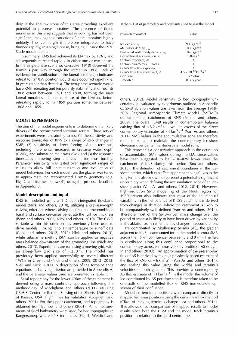
Following results from incremental increases in SM (Fig. 6c),step changes in SM of different magnitudes were appliedonly where the model was spun up with an initial SM rate of0 km3 a–1 at the LIAmax (Fig. 7). The results from these runsdemonstrate that an increase in SM to 0.3 km3 a–1 couldcause a retreat to the 1859 terminus position, though itwould take >200 years to do so. To drive a retreat from theLIAmax to the 1859 position within the time frame observed(<98 years), requires a step-change increase of at least0.5 km3 a–1. However, given the lack of geomorphologicalevidence for a stable margin at 12.5 km, an increase of>0.6 km3 a–1 would probably be required, based on themodelled time needed for the terminus to retreat through the12.5 km pinning point (Fig. 7).

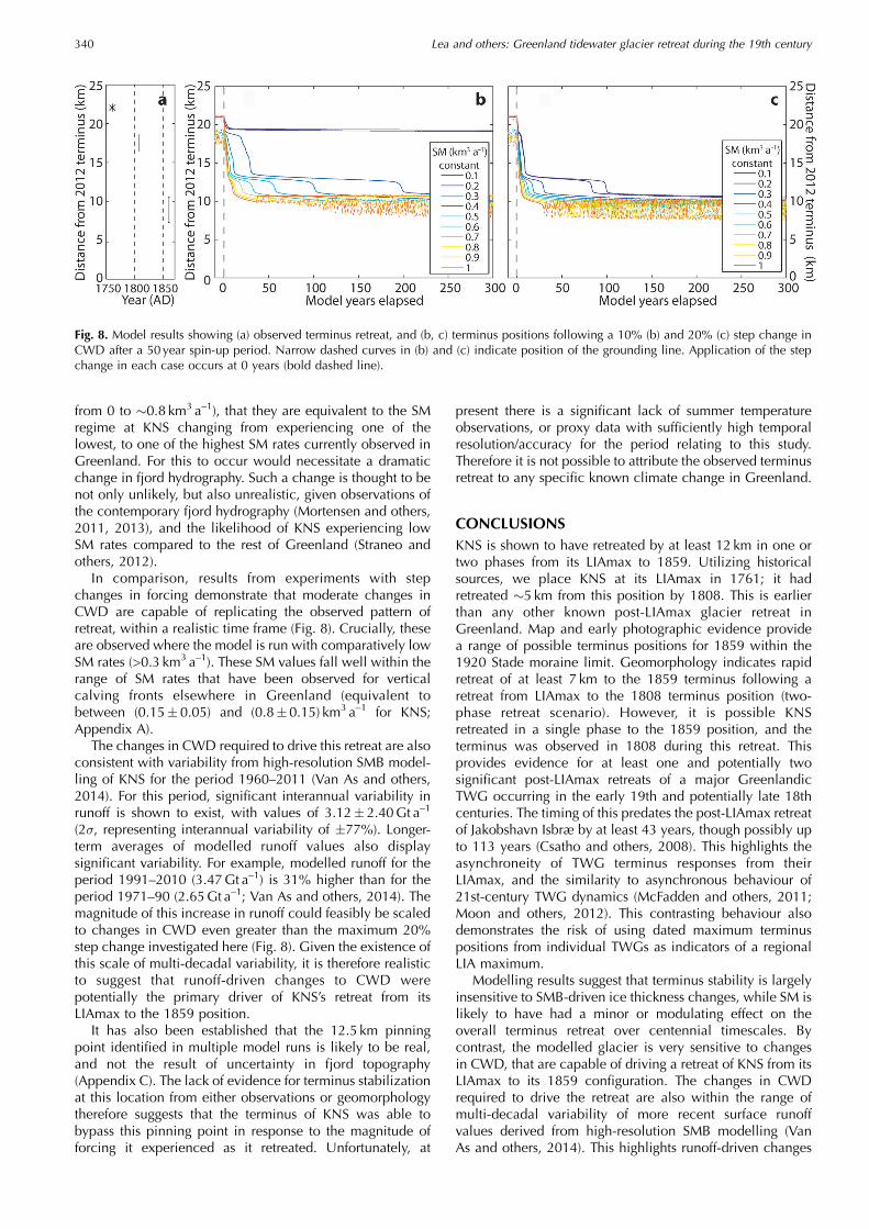
Step changes in CWD of 10% (Fig. 8a) and 20% (Fig. 8b)were also applied for constant SM ranging from 0.1 to1 km3 a–1. As with results from incremental changes inCWD (Fig. 6b), these show that terminus sensitivity tochanges in CWD increases with higher values of SM(Fig. 8). However, results also demonstrate that moderatestep changes in CWD are capable of producing a retreat tothe 1859 position for moderate values of SM. For example,where SM>0.3 km3 a–1, a 20% increase in CWD can drivea retreat from LIAmax to the 1859 position in 31 years.

IMPLICATIONS OF MODEL RESULTS

Model results demonstrate that the LIAmax to 1859 retreat ofKNS is unlikely to have been driven by changes in SM orSMB. Where changes in SM can produce a retreat patterncomparable to that observed (Figs 6c and 7), the SM ratesrequired to achieve this are at the upper end, or greater thananything previously observed in Greenland (Rignot andothers, 2012; Enderlin and Howat, 2013). The step changesin SM required to reproduce observed retreat that skip the12.5 km pinning point are also of such a scale (increasing

Fig. 7.Model results showing (a) observed terminus retreat and (b) terminus position following a step change in SM following a 50 year spin-up period where SM=0km3 a–1, following the results of the incremental sensitivity tests. CWD is held constant throughout (175m). Dashedlines indicate position of the grounding line. Application of the step change in each case occurs at 0 years (bold dashed line).


from 0 to �0.8 km3 a–1), that they are equivalent to the SMregime at KNS changing from experiencing one of thelowest, to one of the highest SM rates currently observed inGreenland. For this to occur would necessitate a dramaticchange in fjord hydrography. Such a change is thought to benot only unlikely, but also unrealistic, given observations ofthe contemporary fjord hydrography (Mortensen and others,2011, 2013), and the likelihood of KNS experiencing lowSM rates compared to the rest of Greenland (Straneo andothers, 2012).

In comparison, results from experiments with stepchanges in forcing demonstrate that moderate changes inCWD are capable of replicating the observed pattern ofretreat, within a realistic time frame (Fig. 8). Crucially, theseare observed where the model is run with comparatively lowSM rates (>0.3 km3 a–1). These SM values fall well within therange of SM rates that have been observed for verticalcalving fronts elsewhere in Greenland (equivalent tobetween (0.15� 0.05) and (0.8�0.15) km3 a–1 for KNS;Appendix A).

The changes in CWD required to drive this retreat are alsoconsistent with variability from high-resolution SMB model-ling of KNS for the period 1960–2011 (Van As and others,2014). For this period, significant interannual variability inrunoff is shown to exist, with values of 3.12� 2.40Gt a–1

(2�, representing interannual variability of �77%). Longer-term averages of modelled runoff values also displaysignificant variability. For example, modelled runoff for theperiod 1991–2010 (3.47Gt a–1) is 31% higher than for theperiod 1971–90 (2.65Gt a–1; Van As and others, 2014). Themagnitude of this increase in runoff could feasibly be scaledto changes in CWD even greater than the maximum 20%step change investigated here (Fig. 8). Given the existence ofthis scale of multi-decadal variability, it is therefore realisticto suggest that runoff-driven changes to CWD werepotentially the primary driver of KNS’s retreat from itsLIAmax to the 1859 position.

It has also been established that the 12.5 km pinningpoint identified in multiple model runs is likely to be real,and not the result of uncertainty in fjord topography(Appendix C). The lack of evidence for terminus stabilizationat this location from either observations or geomorphologytherefore suggests that the terminus of KNS was able tobypass this pinning point in response to the magnitude offorcing it experienced as it retreated. Unfortunately, at

present there is a significant lack of summer temperatureobservations, or proxy data with sufficiently high temporalresolution/accuracy for the period relating to this study.Therefore it is not possible to attribute the observed terminusretreat to any specific known climate change in Greenland.

CONCLUSIONS

KNS is shown to have retreated by at least 12 km in one ortwo phases from its LIAmax to 1859. Utilizing historicalsources, we place KNS at its LIAmax in 1761; it hadretreated �5 km from this position by 1808. This is earlierthan any other known post-LIAmax glacier retreat inGreenland. Map and early photographic evidence providea range of possible terminus positions for 1859 within the1920 Stade moraine limit. Geomorphology indicates rapidretreat of at least 7 km to the 1859 terminus following aretreat from LIAmax to the 1808 terminus position (two-phase retreat scenario). However, it is possible KNSretreated in a single phase to the 1859 position, and theterminus was observed in 1808 during this retreat. Thisprovides evidence for at least one and potentially twosignificant post-LIAmax retreats of a major GreenlandicTWG occurring in the early 19th and potentially late 18thcenturies. The timing of this predates the post-LIAmax retreatof Jakobshavn Isbræ by at least 43 years, though possibly upto 113 years (Csatho and others, 2008). This highlights theasynchroneity of TWG terminus responses from theirLIAmax, and the similarity to asynchronous behaviour of21st-century TWG dynamics (McFadden and others, 2011;Moon and others, 2012). This contrasting behaviour alsodemonstrates the risk of using dated maximum terminuspositions from individual TWGs as indicators of a regionalLIA maximum.

Modelling results suggest that terminus stability is largelyinsensitive to SMB-driven ice thickness changes, while SM islikely to have had a minor or modulating effect on theoverall terminus retreat over centennial timescales. Bycontrast, the modelled glacier is very sensitive to changesin CWD, that are capable of driving a retreat of KNS from itsLIAmax to its 1859 configuration. The changes in CWDrequired to drive the retreat are also within the range ofmulti-decadal variability of more recent surface runoffvalues derived from high-resolution SMB modelling (VanAs and others, 2014). This highlights runoff-driven changes

Fig. 8. Model results showing (a) observed terminus retreat, and (b, c) terminus positions following a 10% (b) and 20% (c) step change inCWD after a 50 year spin-up period. Narrow dashed curves in (b) and (c) indicate position of the grounding line. Application of the stepchange in each case occurs at 0 years (bold dashed line).


to CWD as a likely potential driver of terminus retreatbetween the LIAmax and 1859.

Given the need to establish the centennial-timescalecontrols on TWG variability (and hence ice-sheet response,and likely sea-level change), high-resolution, high-quality,quantitative proxy records of climate forcing are needed toallow adequate evaluation of centennial records of glacierfluctuations, such as presented here. These include recon-structions of local summer air temperature variability (e.g.D’Andrea and others, 2011), runoff (e.g. Kamenos andothers, 2012) and fjord hydrography (e.g. Lloyd and others,2011). The latter is potentially significant for glaciers such asKNS that drain into fjords with a shallow fjord mouth sill(Mortensen and others, 2011, 2013; Straneo and others,2012). Such proxy records, alongside instrumental recordsand longer-term reconstructions of glacier behaviour back totheir Little Ice Age maxima (and where possible beyond),would provide significant improvements to our understand-ing of TWG response over the next 100–200 years.

ACKNOWLEDGEMENTS

We thank two anonymous reviewers for comments thathelped to improve the manuscript. Nora Weitz (University ofMaine, USA) is thanked for assistance with translatingpassages of German, and Christian Koch Madsen (NationalMuseum of Denmark, Copenhagen) for help with trackingdown images of KNS. RACMO2.1 data were provided by Janvan Angelen and Michiel van den Broeke of the Institute forMarine and Atmospheric Research Utrecht (IMAU), TheNetherlands. This research was financially supported byJ.L.’s PhD funding, UK Natural Environment ResearchCouncil (NERC) grant No. NE/I528742/1. Support forF.M.N. was provided by the Conoco-Phillips/Lundin North-ern Area Program CRIOS (Calving Rates and Impact on SeaLevel) project.

REFERENCES

Alley RB and 13 others (2010) History of the Greenland Ice Sheet:paleoclimatic insights. Quat. Sci. Rev., 29(15–16), 1728–1756(doi: 10.1016/j.quascirev.2010.02.007)

Bamber JL, Layberry RL and Gogineni SP (2001) A new icethickness and bed data set for the Greenland ice sheet. 1.Measurement, data reduction, and errors. J. Geophys. Res.,106(D24), 33 773–33 780 (doi: 10.1029/2001JD900054)

Benn DI, Hulton NRJ and Mottram RH (2007) ‘Calving laws’,‘sliding laws’ and the stability of tidewater glaciers. Ann.Glaciol., 46, 123–130 (doi: 10.3189/172756407782871161)

Bevan SL, Luckman AJ and Murray T (2012) Glacier dynamics overthe last quarter of a century at Helheim, Kangerdlugssuaq and14 other major Greenland outlet glaciers. Cryosphere, 6(5),923–937 (doi: 10.5194/tc-6-923-2012)

Bjørk AA and 8 others (2012) An aerial view of 80 years of climate-related glacier fluctuations in southeast Greenland. NatureGeosci., 5(6), 427–432 (doi: 10.1038/ngeo1481)

Box JE and Decker DT (2011) Greenland marine-terminatingglacier area changes: 2000–2010. Ann. Glaciol., 52(59),91–98 (doi: 10.3189/172756411799096312)

Box JE and 11 others (2013) Greenland Ice Sheet mass balancereconstruction. Part I: net snow accumulation (1600–2009).J. Climate, 26(11), 3919–3934 (doi: JCLI-D-12-00373.1)

Briner JP, Stewart HAM, Young NE, Philipps W and Losee S (2010)Using proglacial-threshold lakes to constrain fluctuations of theJakobshavn Isbræ ice margin, western Greenland, during theHolocene. Quat. Sci. Rev., 29(27–28), 3861–3874 (doi:10.1016/j.quascirev.2010.09.005)

Colgan W, Pfeffer WT, Rajaram H, Abdalati W and Balog J (2012)Monte Carlo ice flow modeling projects a new stable config-uration for Columbia Glacier, Alaska, c. 2020. Cryosphere, 6(6),1395–1409 (doi: 10.5194/tc-6-1395-2012)

Cook S, Zwinger T, Rutt IC, O’Neel S and Murray T (2012) Testingthe effect of water in crevasses on a physically based calvingmodel. Ann. Glaciol., 53(60 Pt 1), 90–96 (doi: 10.3189/2012AoG60A107)

Cook S and 6 others (2013) Modelling environmental influences oncalving at Helheim Glacier, East Greenland. Cryos. Discuss.,7(5), 4407–4442 (doi: 10.5194/tcd-7-4407-2013)

Crantz D (1820) The history of Greenland including an account ofthe mission carried on by the united brethren in that country:from the German of David Crantz, 2 vols. Longman, Hurst, Rees,Orme and Brown, London

Csatho B, Schenk T, Van der Veen CJ and Krabill WB (2008)Intermittent thinning of Jakobshavn Isbræ, West Greenland,since the Little Ice Age. J. Glaciol., 53(184), 131–144 (doi:10.3189/002214308784409035)

Cuffey KM and Paterson WSB (2010) The physics of glaciers, 4thedn. Butterworth-Heinemann, Oxford

D’Andrea WJ, Huang Y, Fritz SC and Anderson NJ (2011) AbruptHolocene climate change as an important factor for humanmigration in West Greenland. Proc. Natl Acad. Sci. USA (PNAS),108(24), 9765–9769 (doi: 10.1073/pnas.1101708108)

Enderlin EM and Howat IM (2013) Submarine melt rate estimatesfor floating termini of Greenland outlet glaciers (2000–2010).J. Glaciol., 59(213), 67–75 (doi: 10.3189/2013JoG12J049)

Enderlin EM, Howat IM and Vieli A (2013) The sensitivity offlowline models of tidewater glaciers to parameter uncertainty.Cryosphere, 7(5), 1579–1590 (doi: 10.5194/tc-7-1579-2013)

Ettema J and 6 others (2009) Higher surface mass balance of theGreenland ice sheet revealed by high-resolution climate model-ling. Geophys. Res. Lett., 36(12), L12501 (doi: 10.1029/2009GL038110)

Fowler AC (2010) Weertman, Lliboutry and the development ofsliding theory. J. Glaciol., 56(200), 965–972 (doi: 10.3189/002214311796406112)

Giesecke KL (1910) Mineralogisches Reisejournal uber Gronland1806–13. Medd. Grønl., 35

Gogineni S and 9 others (2001) Coherent radar ice thicknessmeasurements over the Greenland ice sheet. J. Geophys. Res.,106(D24), 33 761–33 772 (doi: 10.1029/2001JD900183)

Holland DM, Thomas RH, De Young B, Ribergaard MH and LyberthB (2008) Acceleration of Jakobshavn Isbræ triggered by warmsubsurface ocean waters. Nature Geosci., 1(10), 659–664 (doi:10.1038/ngeo316)

Jamieson SSR and 6 others (2012) Ice-stream stability on a reversebed slope. Nature Geosci., 5(11), 799–802 (doi: 10.1038/ngeo1600)

Joughin I, Smith BE and Holland DM (2010a) Sensitivity of 21stcentury sea level to ocean-induced thinning of Pine IslandGlacier, Antarctica. Geophys. Res. Lett., 37(20), L20502 (doi:10.1029/2010GL044819)

Joughin I, Smith BE, Howat IM, Scambos T and Moon T (2010b)Greenland flow variability from ice-sheet-wide velocity map-ping. J. Glaciol., 56(197), 415–430 (doi: 10.3189/002214310792447734)

Kamenos NA, Hoey TB, Nienow P, Fallick AE and Claverie T (2012)Reconstructing Greenland ice sheet runoff using coralline algae.Geology, 40(12), 1095–10098 (doi: 10.1130/G33405.1)

Kleinschmidt S (1859) Godthabs distrikt (hertil en Navneliste). (MapNo. KBK Netpublikation RI000074) Copenhagen

Larsen NK, Kjær KH, Olsen J, Funder S, Kjeldsen KK and Nørgaard-Pedersen N (2011) Restricted impact of Holocene climatevariations on the southern Greenland Ice Sheet. Quat. Sci. Rev.,30(21–22), 3171–3180 (doi: 10.1016/j.quascirev.2011.07.022)

Lea JM, Mair DWF and Rea BR (2014) Evaluation of existing andnew methods of tracking glacier terminus change. J. Glaciol.,60(220), 323–332


Lloyd J and 6 others (2011) A 100 yr record of ocean temperaturecontrol on the stability of Jakobshavn Isbræ, West Greenland.Geology, 39(9), 867–870 (doi: 10.1130/G32076.1)

McFadden EM, Howat IM, Joughin I, Smith BE and Ahn Y (2011)Changes in the dynamics of marine terminating outlet glaciers inwest Greenland (2000–2009). J. Geophys. Res., 116(F2), F02022(doi: 10.1029/2010JF001757)

Mercer JH (1961) The estimation of the regimen and former firnlimit of a glacier. J. Glaciol., 3(30), 1053–1062

Moon T and Joughin I (2008) Changes in ice front position onGreenland’s outlet glaciers from 1992 to 2007. J. Geophys. Res.,113(F2), F02022 (doi: 10.1029/2007JF000927)

Moon T, Joughin I, Smith B and Howat I (2012) 21st-centuryevolution of Greenland outlet glacier velocities. Science,336(6081), 576–578 (doi: 10.1126/science.1219985)

Morlighem M, Rignot E, Seroussi H, Larour E, Ben Dhia H andAubry D (2011) A mass conservation approach for mappingglacier ice thickness. Geophys. Res. Lett., 38(19), L19503 (doi:10.1029/2011GL048659)

Mortensen J, Lennert K, Bendtsen J and Rysgaard S (2011) Heatsources for glacial melt in a sub-Arctic fjord (Godthabsfjord) incontact with the Greenland Ice Sheet. J. Geophys. Res., 116(C1),C01013 (doi: 10.1029/2010JC00652)

Mortensen J and 6 others (2013) On the seasonal freshwaterstratification in the proximity of fast-flowing tidewater outletglaciers in a sub-Arctic sill fjord. J. Geophys. Res., 118(3),1382–1395 (doi: 10.1002/jgrc.20134)

Murray T and 10 others (2010) Ocean regulation hypothesis forglacier dynamics in southeast Greenland and implications forice sheet mass changes. J. Geophys. Res., 115(F3), F03026 (doi:10.1029/2009JF001522)

Nick FM, Vieli A, Howat IM and Joughin I (2009) Large-scalechanges in Greenland outlet glacier dynamics triggered at theterminus.Nature Geosci., 2(2), 110–114 (doi: 10.1038/ngeo394)

Nick FM, Van der Veen CJ, Vieli A and Benn DI (2010) A physicallybased calving model applied to marine outlet glaciers andimplications for the glacier dynamics. J. Glaciol., 56(199),781–794 (doi: 10.3189/002214310794457344)

Nick FM and 8 others (2012) The response of Petermann Glacier,Greenland, to large calving events, and its future stability in thecontext of atmospheric and oceanic warming. J. Glaciol.,58(208), 229–239 (doi: 10.3189/2012JoG11J242)

Nick FM and 7 others (2013) Future sea-level rise from Greenland’smajor outlet glaciers in a warming climate. Nature, 497(7448),235–238 (doi: 10.1038/nature12068)

Nye JF (1957) The distribution of stress and velocity in glaciers andice-sheets. Proc. R. Soc. London, Ser. A, 239(1216), 113–133(doi: 10.1098/rspa.1957.0026)

Rignot E, Koppes M and Velicogna I (2010) Rapid submarinemelting of the calving faces of West Greenland glaciers. NatureGeosci., 3(3), 141–218 (doi: 10.1038/ngeo765)

Rignot E, Fenty I, Menemenlis D and Xu Y (2012) Spreading ofwarm ocean waters around Greenland as a possible cause forglacier acceleration. Ann. Glaciol., 53(60 Pt 2), 257–266 (doi:10.3189/2012AoG60A136)

Rink H (1856) Sydgrønlands nordlige distrikter. (Map No. KBKNetpublikation RI000095) Copenhagen

Sciascia R, Straneo F, Cenedese C and Heimbach P (2013) Seasonalvariability of submarine melt rate and circulation in an EastGreenland fjord. J. Geophys. Res., 118(C5), 2492–2506 (doi:10.1002/jgrc.20142)

Straneo F and 7 others (2010) Rapid circulation of warm subtropicalwaters in a major glacial fjord in East Greenland. NatureGeosci., 3(33), 182–186 (doi: 10.1038/ngeo764)

Straneo F and 8 others (2012) Characteristics of ocean watersreaching Greenland’s glaciers. Ann. Glaciol., 53(60 Pt 2),202–210 (doi: 10.3189/2012AoG60A059)

Thomas RH (2004) Force-perturbation analysis of recent thinningand acceleration of Jakobshavn Isbræ, Greenland. J. Glaciol.,50(168), 57–66 (doi: 10.3189/172756504781830321)

Thorhallesen E (1776) Efterretning om rudera eller levninger af degamle nordmœnds og islœnderes bygninger paa Grønlandsvester-side, tilligemed et anhang om deres undergang samme-steds. Trykt hos A.F. Stein, Copenhagen

Van As D, Hubbard AL, Hasholt B, Mikkelsen AB, Van den BroekeMR and Fausto RS (2012) Large surface meltwater dischargefrom the Kangerlussuaq sector of the Greenland ice sheet duringthe record-warm year 2010 explained by detailed energybalance observations. Cryosphere, 6(1), 199–209 (doi:10.5194/tc-6-199-2012)

Van As D and 11 others (2014) Increasing meltwater discharge fromthe Nuuk region of the Greenland ice sheet and implications formass balance (1960–2012). J. Glaciol., 60(220), 314–322

Van den Broeke M and 8 others (2009) Partitioning recentGreenland mass loss. Science, 326(5955), 984–986 (doi:10.1126/science.1178176)

Van der Veen CJ and Whillans IM (1996) Model experiments on theevolution and stability of ice streams. Ann. Glaciol., 23,129–137

Vieli A and Nick FM (2011) Understanding and modelling rapiddynamic changes of tidewater outlet glaciers: issues andimplications. Surv. Geophys., 32(4–5), 437–458 (doi: 10.1007/s10712-011-9132-4)

Vinther BM, Andersen KK, Jones PD, Briffa KR and Cappelen J(2006) Extending Greenland temperature records into the lateeighteenth century. J. Geophys. Res., 111(D11), D11105 (doi:10.1029/2005JD006810)

Weidick A (1959) Glacial variations in West Greenland in historicaltime. Part I. South West Greenland. Bull. Grønl. Geol. Unders.18

Weidick A (1968) Observations on some Holocene glacierfluctuations in West Greenland. Medd. Grønl. 165(6)

Weidick A and Bennike O (2007) Quaternary glaciation history andglaciology of Jakobshavn Isbræ and the Disko Bugt region, WestGreenland: a review. Geol. Surv. Den. Greenl. Bull. 14

Weidick A and Citterio M (2011) Correspondence. The ice-dammedlake Isvand, West Greenland, has lost its water. J. Glaciol.,57(201), 186–188 (doi: 10.3189/002214311795306600)

Weidick A, Bennike O, Citterio M and Nørgaard-Pedersen N (2012)Neoglacial and historical glacier changes around KangersuneqFjord in southern West Greenland. Geol. Surv. Den. Greenl.Bull. 27

APPENDIX A: MODEL DESCRIPTION

The model used in this study is designed to simulate thebehaviour of tidewater outlet glaciers, and is explained infull detail in Nick and others (2010). It employs a simple,physically based, nonlinear effective pressure sliding law,where the depth-integrated driving stress is balanced bylongitudinal stress gradients, basal and lateral drag (Van derVeen and Whillans, 1996; Fowler, 2010). These are repre-sented by the first, second and third terms respectively onthe right-hand side of Eqn (A1), with the driving stressrepresented by the left-hand term:

�igH@H

@x¼ 2

@

@xH�

@U

@x

� �� As H � �p

�iD

� �U

� �1=m

� 2H

W

5U

�AW

� �1=m

ðA1Þwhere �i is density of ice, �p is density of the proglacial waterbody, g is gravitational acceleration, x is the along-flowdistance, H is ice thickness, D is depth of ice below thesurface of the proglacial water body, As is bed roughnessparameter, A is temperature-dependent rate factor (4.5�10–17 Pa–3 a–1, corresponding to ice at –58C (Cuffey and


Paterson, 2010)), W is glacier width, � is effective viscosity(dependent on the strain rate) and m is friction exponent.This sliding law allows the modelled glacier to replicate thevelocity profiles that are often observed approaching marinetermini, and thus provides a good representation of realisticsliding (Nick and others, 2010, 2013; Vieli and Nick, 2011;Jamieson and others, 2012). Constant and parameter valuesused in the model are outlined in Table 1.

Variations in basal and lateral friction due to meltwatersupply can also potentially be modelled using the frictionparameters � and � (Nick and others, 2010, 2012, 2013).However, both are given a constant value of 1 in all modelruns shown, since this has primarily been suggested to bemost significant over sub-annual, rather than multi-annual todecadal, timescales (Howat and others, 2010; Nick andothers, 2010, 2012, 2013; Vieli and Nick, 2011).

The model employs a full-depth calving criterion, calcu-lating the penetration depth of both surface and basalcrevasses within a field of closely spaced crevasses (Nye,1957; Benn and others, 2007). Calving occurs when thesurface and basal crevasses combined penetrate the full icethickness (Nick and others, 2010). Where water ponds increvasses there is the potential for it to force deeperpenetration compared to a dry crevasse, according to

ds ¼2

�ig

_"xxA

� �1=n

þ �w�i

dw ðA2Þ

where ds is depth of surface crevasse, _"xx is longitudinalstretching rate, n is Glen’s flow law exponent and dw iscrevasse water depth. For a given flow regime, greater valuesof dw can therefore instigate higher calving rates that in turndrive retreat.

Basal crevasse heights are also included in calculations ofcumulative crevasse penetration, according to

db ¼2�i

�p � �i

_"xxA

� �1=n 1

�ig�Hab

� �ðA3Þ

whereHab is height above buoyancy of a given ice thickness,calculated as

Hab ¼ H � �p

�iD ðA4Þ

This full-depth calving criterion is employed given thatinstances of full-depth calving behaviour were observed atKNS during fieldwork conducted in August 2011.

SM is applied uniformly across the entire width of thegrounding line. Volumetric rates of SM (e.g. km3 a–1) are alsoprescribed within the model rather than linear melt rates pertime-step (e.g. md–1). This is because application of thelatter to a 1-D model will result in SM volume being partiallydependent on the glacier width. Volumetric rates provideinternal consistency between model runs for each time-stepand location in the modelled fjord. Constant SM valuesranged from 0 to 1.5 km3 a–1 (0.1 km3 a–1 intervals). Thelatter is equivalent to SM rates of 0 to �5.25md–1 withincrements of �0.36md–1. This covers the range of valuesup to 150% of those that have so far been observed fortermini in western Greenland (Rignot and others, 2012;Enderlin and Howat, 2013).

To allow direct comparison, previously published dailylinear SM rate values (md–1) were multiplied by 365.25 toscale them up to units of m a–1, before being converted tovolumetric values. The conversion to volumetric melt rateswas achieved by multiplying the annual linear SM values by

KNS’s contemporary glacier width (�5 km) and fjord depth atthe terminus (�225m). As an approximation, these SMvolume values were then halved, to reflect that the majorityof SM occurs during summer only, driven by subglacial runoff(Sciascia and others, 2013). These equate to volumetric SMrange estimates for KNS of between (0.15� 0.05) and(0.8�0.15) km3 a–1 (Rignot and others, 2012; Enderlin andHowat, 2013). Within this range, the SM value for KNS hasbeen suggested to be low compared to other Greenlandicglaciers, since fjord bathymetry is thought to limit the influ-ence of ocean waters on fjord water temperature (Mortensenand others, 2011, 2013; Straneo and others, 2012).

APPENDIX B: MODEL TUNING

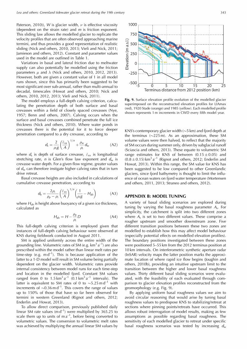
A variety of basal sliding scenarios are explored duringtuning by varying the basal roughness parameter As. Forsimplicity, the catchment is split into two different zoneswhere As is set to two different values. These comprise arougher upstream and smoother downstream zone. Fivedifferent transition positions between these two zones aremodelled to establish how this may affect model behaviour(especially potential effects on modelled elevation profiles).The boundary positions investigated between these zoneswere positioned 5–55 km from the 2012 terminus position at10 km intervals. On interferometric synthetic aperture radar(InSAR) velocity maps the latter position marks the approxi-mate location of where rapid ice flow begins (Joughin andothers, 2010b), providing an intuitive upstream limit to thetransition between the higher and lower basal roughnessvalues. Thirty different basal sliding scenarios were evalu-ated, with the feasibility of each evaluated through com-parison to glacier elevation profiles reconstructed from thegeomorphology (e.g. Fig. 9).

By applying uniform basal roughness values we aim toavoid circular reasoning that would arise by tuning basalroughness values to predispose KNS to stabilizing/retreat atsections where pinning points/retreats have occurred. Thisallows robust interrogation of model results, making as fewassumptions as possible regarding basal roughness. Thesensitivity of each modelled glacier to retreat under specificbasal roughness scenarios was tested by increasing dw

Fig. 9. Surface elevation profile evolution of the modelled glaciersuperimposed on the reconstructed elevation profiles for LIAmax(red), 1920 Stade (orange) and 1985 (yellow). Each modelled profileshown represents 1m increments in CWD every fifth model year.


incrementally. For each scenario the post-spin-up value ofdw was increased by 1m every 5 model years until theterminus retreated beyond the 2012 terminus position, or dwexceeded 250m. The latter condition is applied sincesections of the fjord are <250m in depth, meaning that inthese regions the terminus is fully grounded and its positionwill be defined almost solely as a function of dw. Where thisoccurs and the fjord continues to shallow this could

potentially force the creation of unrealistic freeboard heightsat modelled termini.

Figure 9 is an example output of the sensitivity tests,showing the profile evolution of the basal roughnessconfiguration used in this study.

APPENDIX C: BED SENSITIVITY

Previously published work has established that model resultsof tidewater glaciers can be sensitive to uncertainties in fjordbathymetry (Enderlin and others, 2013). To evaluate whetherthe uncertainty in fjord bathymetry significantly affectsmodelled terminus behaviour, sensitivity tests were con-ducted. This involved randomly varying bed elevation wherefjord topography is unknown over blocks of three gridcells(�750m), across a vertical range of �50m, before thenbeing smoothed over the same distance to avoid stepchanges in topography. Three sets of experiments were run,(1) varying the bed downstream of the 1920 Stade max-imum, holding the downstream section of the fjord constant,(2) varying the bed upstream of the 1920 Stade maximum,holding the upstream section of the fjord constant, and(3) varying the bed downstream of the 2012 terminusposition. This evaluates the impact of bed uncertainty, andpotentially the section of the fjord where this is important.Each experiment was run for 50 different bed configurations.

Results demonstrate that unknown sections of fjordtopography do not significantly affect the large-scale retreatbehaviour of KNS (e.g. Fig. 10). Pinning points identified bythe model are therefore suggested to be real, rather thanartefacts of fjord topography uncertainty.

Fig. 10. Example of terminus sensitivity to random changes inunknown sections of fjord bathymetry along the entire length of thefjord. Results are shown for the retreat pattern of the modelledglacier in response to 1m increments of CWD every fifth modelyear, for 50 different bed configurations.

MS received 22 August 2013 and accepted in revised form 18 January 2014


Terminus-driven retreat of a major southwest Greenland ...

Documents

Transcript of Terminus-driven retreat of a major southwest Greenland ...