Term Structure of Consumption Risk Premia in the Cross Section of ...
38
THE JOURNAL OF FINANCE • VOL. LXXII, NO. 4 • AUGUST 2017 Term Structure of Consumption Risk Premia in the Cross Section of Currency Returns IRINA ZVIADADZE ∗ ABSTRACT I relate the downward-sloping term structure of currency carry returns to compensa- tion for currency exposures to macroeconomic risk embedded in the joint dynamics of U.S. consumption, inflation, nominal interest rate, and their stochastic variance. The interest rate and inflation shocks play a prominent role. Higher yield currencies ex- hibit higher multiperiod exposures to these shocks. The prices of these risk exposures are positive and sizeable across all investment horizons. The interest rate shock is qualitatively similar to the long-run risk of Bansal and Yaron. IN THIS PAPER,I QUANTIFY THE RISK-RETURN relationship in the foreign exchange (FX) market across different countries and investment horizons. My starting point is new evidence about returns on a currency carry trade, a zero-cost investment strategy that entails buying bonds in high-yield currencies and short-selling bonds in low-yield currencies, across alternative investment hori- zons. The term structure of average carry log returns is slightly downward sloping: the average log returns are 1.13% and 0.80% per quarter at the three- month and 10-year investment horizon, respectively. I ask which sources of macroeconomic risk are compensated in the term structure of carry returns. Shocks to consumption growth, inflation, interest rates, and their second- order moments reflect different aspects of currency risk. My focus is on iden- tifying such shocks, measuring their impact on exchange rates in the cross ∗ Zviadadze is at the Stockholm School of Economics. I am grateful to the Editor, Kenneth Single- ton, the anonymous Associate Editor, and two referees for constructive feedback. I am indebted to my advisors, Mikhail Chernov and Francisco Gomes, for their unconditional support, stimulating discussions, and helpful suggestions. I am also grateful to David Backus, Tomas Bjork, Jaroslav Boroviˇ cka, Laurent Calvet, Joao Cocco, Riccardo Colacito, Mariano M. Croce, Magnus Dahlquist, David Edgerton, Vito Gala, Jeremy Graveline, Lars Hansen, Christian Heyerdahl-Larsen, Chris- tian Julliard, Leonid Kogan, Lars Lochstoer, Igor Makarov, Michael Moore, Ivan Shaliastovich, Paolo Surico, Stijn Van Nieuwerburgh, Christian Wagner, and Stanley Zin for advice and detailed feedback. I further thank many participants of conferences and seminars, including Early Career Women in Finance, Frontiers of Finance Warwick, SED, SoFiE, Young Scholars Nordic Finance Workshop, WFA, World Congress of Econometric Society, Bocconi, HEC Paris, LBS, LSE, Lund Uni- versity, New Economic School, Rutgers Business School, Stockholm School of Economics, Sveriges Riksbank, UNC Kenan-Flagler Business School, and UCLA Anderson School of Management, for many helpful discussions and comments. I gratefully acknowledge financial support from the AXA research fund, Jan Wallander and Tom Hedelius Foundation, and Swedish House of Finance. The author has no conflicts of interest, as identified in the Disclosure Policy. DOI: 10.1111/jofi.12501 1529
Transcript of Term Structure of Consumption Risk Premia in the Cross Section of ...
THE JOURNAL OF FINANCE • VOL. LXXII, NO. 4 • AUGUST 2017
Term Structure of Consumption Risk Premiain the Cross Section of Currency Returns
IRINA ZVIADADZE∗
ABSTRACT
I relate the downward-sloping term structure of currency carry returns to compensa-tion for currency exposures to macroeconomic risk embedded in the joint dynamics ofU.S. consumption, inflation, nominal interest rate, and their stochastic variance. Theinterest rate and inflation shocks play a prominent role. Higher yield currencies ex-hibit higher multiperiod exposures to these shocks. The prices of these risk exposuresare positive and sizeable across all investment horizons. The interest rate shock isqualitatively similar to the long-run risk of Bansal and Yaron.
IN THIS PAPER, I QUANTIFY THE RISK-RETURN relationship in the foreign exchange(FX) market across different countries and investment horizons. My startingpoint is new evidence about returns on a currency carry trade, a zero-costinvestment strategy that entails buying bonds in high-yield currencies andshort-selling bonds in low-yield currencies, across alternative investment hori-zons. The term structure of average carry log returns is slightly downwardsloping: the average log returns are 1.13% and 0.80% per quarter at the three-month and 10-year investment horizon, respectively. I ask which sources ofmacroeconomic risk are compensated in the term structure of carry returns.
Shocks to consumption growth, inflation, interest rates, and their second-order moments reflect different aspects of currency risk. My focus is on iden-tifying such shocks, measuring their impact on exchange rates in the cross
∗Zviadadze is at the Stockholm School of Economics. I am grateful to the Editor, Kenneth Single-ton, the anonymous Associate Editor, and two referees for constructive feedback. I am indebted tomy advisors, Mikhail Chernov and Francisco Gomes, for their unconditional support, stimulatingdiscussions, and helpful suggestions. I am also grateful to David Backus, Tomas Bjork, JaroslavBorovicka, Laurent Calvet, Joao Cocco, Riccardo Colacito, Mariano M. Croce, Magnus Dahlquist,David Edgerton, Vito Gala, Jeremy Graveline, Lars Hansen, Christian Heyerdahl-Larsen, Chris-tian Julliard, Leonid Kogan, Lars Lochstoer, Igor Makarov, Michael Moore, Ivan Shaliastovich,Paolo Surico, Stijn Van Nieuwerburgh, Christian Wagner, and Stanley Zin for advice and detailedfeedback. I further thank many participants of conferences and seminars, including Early CareerWomen in Finance, Frontiers of Finance Warwick, SED, SoFiE, Young Scholars Nordic FinanceWorkshop, WFA, World Congress of Econometric Society, Bocconi, HEC Paris, LBS, LSE, Lund Uni-versity, New Economic School, Rutgers Business School, Stockholm School of Economics, SverigesRiksbank, UNC Kenan-Flagler Business School, and UCLA Anderson School of Management, formany helpful discussions and comments. I gratefully acknowledge financial support from the AXAresearch fund, Jan Wallander and Tom Hedelius Foundation, and Swedish House of Finance. Theauthor has no conflicts of interest, as identified in the Disclosure Policy.
DOI: 10.1111/jofi.12501
1529

1530 The Journal of Finance R©
section and at alternative horizons, and understanding their relative impor-tance for carry trade profitability across alternative investment horizons. Ifind that interest rate and inflation shocks play a prominent role. Higher yieldcurrencies exhibit higher multiperiod exposures to these shocks. The prices ofthese risk exposures are positive and sizeable across all investment horizons.The interest rate shock contributes most to cross-sectional differences in cur-rency returns across multiple investment horizons and operates qualitativelysimilarly to the long-run risk of Bansal and Yaron (2004).
My analysis proceeds in two stages. In the first stage, I describe the empir-ical properties of currency risk related to macroeconomic fluctuations. To thisend, I estimate the joint dynamics of U.S. consumption growth, inflation, thenominal interest rate, and the cross section of exchange rate growth as a vec-tor autoregression (VAR) with stochastic variance. I compute shock exposureelasticities (Borovicka et al. (2011), Borovicka and Hansen (2014), Zviadadze(2016)) of exchange rates to measure the importance of macroeconomic shocksidentified from the VAR. Shock exposure elasticities are marginal multiperiodsensitivities of exchange rates to alternative current-period shocks. Intuitively,a source of risk is economically interesting if the shock exposure elasticities oflow and high interest rate currencies exhibit high dispersion at alternativehorizons.
I document economically sizeable and statistically significant gaps betweenthe shock exposure elasticities in the cross section of currency baskets. Higheryield currencies exhibit higher exposures to the interest rate and inflationshocks across multiple investment horizons. To the best of my knowledge, thisis the first study to explicitly relate interest rate and inflation shocks, identifiedfrom U.S. macroeconomic data, to the cross section of currency baskets, and toexplore the term structure of currency exposures to macroeconomic risk. Thesenovel facts complement the influential evidence of Lustig and Verdelhan (2007)in a nontrivial way.
The dispersion in multiperiod currency exposures to the sources of risk isa necessary but not sufficient condition for relating the cross-sectional spreadin currency returns across alternative investment horizons to macroeconomicrisk. An open question is whether currency sensitivities to risk have an eco-nomically sizeable price. This is where the second stage of my analysis comesin. To measure price of risk, I introduce a U.S. representative agent with recur-sive utility and an aversion to consumption risk, and I interpret the estimatedVAR as a model of consumption growth with the explicitly specified dynamicsof expected consumption growth and stochastic variance. Consequently, themacroeconomic shocks represent multiple sources of consumption risk.
Combining the VAR with recursive preferences comes with its challenges.The nominal yield plays a dual role. On the one hand, the pricing kernel de-pends on the nominal yield, as it is one of the state variables in the model.On the other hand, the nominal yield is the (log) conditional expectation of thepricing kernel and hence an affine function of the model’s states. The first-ordercondition implies a set of pricing restrictions on the structural parameters ofthe model. The structural restrictions imposed on the parameters of the VAR
Term Structure of Consumption Risk Premia 1531
lead to nontrivial complications in estimation that I resolve by using BayesianMarkov Chain Monte Carlo (MCMC) methods.
Armed with the estimated dynamics of the pricing kernel, I characterizehow currency sensitivities to macroeconomic risk are compensated in the mar-ketplace at horizons from one quarter to 10 years. Shock price elasticities(Borovicka et al. (2011), Borovicka and Hansen (2014), Zviadadze (2016)) as-sign prices to shock exposure elasticities. Put simply, shock price elasticitiesconstitute a term structure of marginal prices of risk, or a term structure ofmarginal Sharpe ratios.
The analysis of the shock elasticities reveals that interest rate risk plays themost prominent role in the FX market. Two important properties lead to thisconclusion. First, I confirm in the context of the structural VAR that higher yieldcurrencies exhibit larger sensitivities to the shock at horizons from one quarterto 16 quarters.1 This fact means that, upon realization of the positive shock,high-yield currencies are expected to appreciate relative to low-yield currenciesover a four-year period. Second, the marginal price for bearing interest rate riskis the largest at all investment horizons. Taken together, the evidence suggeststhat the term structure of currency risk premia reflects the interest rate shockat short- and medium-term horizons.
An examination of the empirical properties of the interest rate shock sug-gests that this risk is qualitatively similar to the long-run risk of Bansal andYaron (2004). First, the shock affects consumption growth only with a lag ofone quarter. Second, the shock originates via a persistent variable and has thehighest price of risk. Finally, it is the dominant source of variation in the realrisk-free rate. These empirical results complement the argument of Colacitoand Croce (2013) about the special role of long-run risk in currency markets.Their conclusion is based on a symmetric two-country setting that, by construc-tion, does not accommodate the term structure of the cross-sectional spreadsin currency risk premia. I leave identification of the economic origins of thelong-run risk shock operating in the FX market for future research.
Estimation of the structural VAR reveals that, similar to the case of the in-terest rate shock, higher yield currencies have higher exposures to the inflationshock across multiple investment horizons. The marginal price of the shock isless sizeable than that of the interest rate shock but is economically mean-ingful. Given the quantitative prominence of the inflation shock in the termstructure of currency carry premia, future models of FX risk should explore notonly real (as has been the main focus so far) but also nominal sources of risk.
The variance shock contributes to the term structure of currency risk premiain a conceptually different way. Currencies are not sensitive to the varianceshock at any investment horizon, yet it is the only source of time-variationin the risk premium. As a result, the log expected return on the one-periodcarry trade strategy, for example, has fluctuated between 0.43% and 3.54% perquarter.
1 Henceforth, I use the structural VAR and the VAR augmented with cross-equation restrictionsinterchangeably.

1532 The Journal of Finance R©
The role of the consumption growth shock is limited to high-yield currenciesat the one-period investment horizon. The average price for bearing a three-month exposure of high-yield currencies to the consumption growth shock isabout 0.24% per quarter. Thanks to the high compensation of the one-periodexposure of high-yield currencies to the consumption growth shock, the carryrisk premium is largest at the three-month investment horizon.
The cross section of currency risk premia as compensation for currency ex-posures to macroeconomic risk exhibits a downward-sloping term structure.At the short- and medium-term end, the carry risk premia are rather flat andreach about 1.31% per quarter, on average. At horizons longer than 10 quarters,the risk premia are statistically insignificant. Hence, the profitability of invest-ments in bonds of high interest rate currencies, when the money is borrowedin low interest rate environments, is a short- to medium-horizon phenomenon.
This paper is related to the international macrofinance literature that exam-ines time-series and cross-sectional properties of currency risk premia. I limitthe discussion here to papers that interpret currency risk premia as compensa-tion for macroeconomic risk. On the empirical side, Cumby (1988), Lustig andVerdelhan (2007), and Sarkissian (2003) study the ability of the consumptiongrowth factor to explain the cross section of currency returns. The authors con-sider different cross sections of currency returns: Cumby (1988) and Sarkissian(2003) study individual currencies, whereas Lustig and Verdelhan (2007) ex-amine interest rate–sorted currency portfolios.
Cumby (1988) shows that ex ante currency returns and conditional covari-ances between currency excess returns and U.S. consumption growth connect ina way that is consistent with consumption-based models. Formal testing, how-ever, reveals that basic models—for example, models with a time-separableutility function—cannot quantitatively account for the behavior of currencyreturns.
Sarkissian (2003) adapts the framework of Constantinides and Duffie (1996)to a multicountry setting and shows that the cross-country variance of con-sumption growth has explanatory power for cross-sectional differences in re-turns on individual currencies, whereas consumption growth itself does not.Lustig and Verdelhan (2007) use the framework of the durable consumptioncapital asset pricing model (CCAPM) of Yogo (2006) to establish that consump-tion growth is a priced factor in the cross section of returns on currency basketsformed by sorting currencies by respective interest rates.
Sarkissian (2003) and Lustig and Verdelhan (2007) have two commonthreads. First, both studies recognize the presence of multiple sources of con-sumption risk but do not describe them explicitly. Second, neither paper extendsthe analysis beyond a single horizon given by the decision interval of the rep-resentative agent (one quarter in the case of Sarkissian (2003), and one yearin the case of Lustig and Verdelhan (2007)). My study fills this void by linkingthe profitability of interest rate–sorted currency portfolios to multiple sourcesof consumption risk across alternative investment horizons.
The theoretical literature features different macro-based models dedicatedto rationalizing the time-variation in currency log returns, for example, the

Term Structure of Consumption Risk Premia 1533
violation of uncovered interest rate parity (UIP) (Fama (1984) regressions).The models include settings with habits (Verdelhan (2010), Heyerdahl-Larsen(2014)), long-run risks (Colacito (2009), Bansal and Shaliastovich (2013),Colacito and Croce (2013)), and disasters (Farhi and Gabaix (2016)). This pa-per builds on important lessons drawn from the international long-run riskliterature, yet makes a number of complementary independent contributions.For example, an influential paper by Colacito and Croce (2011) suggests a linkbetween international long-run risk and exchange rate movements. My empir-ical results confirm the importance of this economic mechanism from a novelperspective: I document the multiperiod heterogeneous risk exposures of lowand high-yield currencies to the domestic interest rate shock that operatesqualitatively similarly to long-run risk. The two-country symmetric theoreticalmodel of Colacito and Croce (2011) does not imply the presence of such a crosssection of currency risk exposures across alternative investment horizons (seeexpression (5) in their paper).
My paper also adds to a rapidly growing literature on the term structures ofvarious assets. So far there has been no explicit study of the effect of the invest-ment horizon on the profitability of carry trades. Recently, Lustig, Stathopoulos,and Verdelhan (2016) analyzed the profitability of investing in bonds of differ-ent maturities across the globe over one period. They document lower averagereturns on strategies involving longer term bonds and rely on the assumptionof market completeness to interpret this fact as a manifestation of the sta-tionarity of exchange rates. Furthermore, they establish a connection betweenstationarity of exchange rates and UIP at an infinite investment horizon.
I characterize the term structure of average carry log returns and explainits shape and level in a flexible consumption-based model of a representativeagent with recursive preferences without relying on the assumption of mar-ket completeness. My analysis is silent about the properties of the investmentstrategy considered by Lustig, Stathopoulos, and Verdelhan (2016), as I delib-erately choose not to model the foreign pricing kernel. Thus, I see my studyand the paper by Lustig, Stathopoulos, and Verdelhan (2016) as complemen-tary sources of evidence on multiperiod profitability of investment strategiesinvolving trades in bonds of different countries and different maturities.
My analysis delivers empirical facts that future general equilibrium modelsof currency risk should account for: (i) interest rate and inflation shocks arereflected in the term structure of carry returns, (ii) the interest rate shockplays the most prominent role in currency pricing, and (iii) the interest rateshock operates qualitatively similarly to the long-run risk of Bansal and Yaron(2004). In addition, my findings emphasize the presence of asymmetry acrosscountries, as highlighted earlier by Backus, Foresi, and Telmer (2001) andLustig, Roussanov, and Verdelhan (2011), among others, and the prominenceof not only real but also nominal risk in the FX market.
Finally, my paper is related to Hansen, Heaton, and Li (2008), who provideevidence of the importance of the permanent shock to consumption in account-ing for the value premium. While both papers use a similar methodology ofmodeling the pricing kernel (under the assumption of recursive preferences)

1534 The Journal of Finance R©
jointly with asset cash flows, my study differs from Hansen, Heaton, and Li(2008) along three principal dimensions. First, I study the FX market, whichhas been examined to a lesser degree than the U.S. equity market. Second, mymodel has stochastic variance: I account for the variation in the volatility ofconsumption growth and therefore in risk premia. Third, I quantify the relativeimportance of consumption shocks for short and medium horizons, rather thanat an infinite horizon.
The paper is organized as follows. Section I presents evidence on the termstructure of average carry log returns and empirically analyzes in reduced formhow the dynamics of the cross section of exchange rates relates to macroeco-nomic shocks. Section II develops an equilibrium framework for studying howthe term structure of currency returns reflects multiple sources of consumptionrisk and discusses the estimation methodology. Section III documents the esti-mation results—(i) the term structure of consumption risk in the cross sectionof currency baskets, (ii) the term structure of prices of consumption shocksin the cross section of currency baskets, and (iii) the term structure of con-sumption risk premia in the cross section of currency returns—and discussesthe economic underpinnings of FX risk. Section IV concludes. Four appendicescontain a description of the data set, the solution to the model, and estimationoutput. The Internet Appendix contains supplementary robustness checks andvarious methodological details.2
I. Macroeconomic Risk in the Cross Section of Exchange Rates
A. Multiperiod Profitability of Carry Trades
I explore the term structure of average carry log returns with holding pe-riods ranging from one quarter to 10 years. At the end of each quarter, thecurrencies of 12 large economies are sorted based on their interest rates andallocated to three equally weighted baskets: basket “Low” (low interest ratecurrencies), basket “Intermediate” (intermediate interest rate currencies), andbasket “High” (high interest rate currencies). The cross-term foreign interestrate
it = 1T
T∑τ=1
it,t + τ
serves as a sorting variable where T = 40 denotes the number of maturitiesin the foreign term structure and it,t+τ denotes a foreign yield of maturity τ
periods (quarters) at time t.3 Because the average yield aggregates informationfrom the entire yield curve, this sorting separates low and high interest ratecurrencies across different investment horizons. A unit investment horizon isone quarter. Table I presents the dynamic composition of currency baskets;Appendix A describes the sample and data sources.
2 An Internet Appendix may be found in the online version of this article.3 In what follows, a tilde denotes foreign variables.

Term Structure of Consumption Risk Premia 1535
Table IComposition of Currency Baskets
This table shows the number of periods for which an individual currency belongs to a basket. The
three baskets are formed by sorting currencies by cross-term interest rates it = 1T
T∑τ=1
it,t+τ , where
T = 40 is the number of maturities in the term structure, it,t+τ is a foreign yield of maturity τ
periods (quarters) at time t. The data are quarterly over the period 1986Q2 to 2011Q4. Basketsare rebalanced quarterly.
Number of Periods in Currency Basket
Currency of “Low” “Intermediate” “High”
Australia 0 23 76Canada 20 75 8Denmark 11 70 12Euro area 17 12 0Germany 34 16 2Japan 103 0 0New Zealand 4 10 73Norway 1 24 30South Africa 0 0 58Sweden 32 29 15Switzerland 95 0 0United Kingdom 5 50 48
An investor follows a simple investment strategy. She borrows U.S. dollars atthe τ -period risk-free rate it,t+τ , converts the money into the foreign currenciesof one of the baskets, buys τ -period foreign risk-free bonds, and at time t + τ
converts the proceeds back into U.S. dollars to pay off the debt. The log excessreturn for this strategy applied to an individual foreign currency is
log rxt,t+τ = log st+τ − log st + it,t+τ − it,t+τ ,
where the exchange rate st is the nominal price of a foreign currency in U.S.dollars. The log excess return for a currency basket is the equal-weightedaverage log excess return across all currencies in the basket.
I use the relationship between average log excess returns and yields high-lighted by Backus, Boyarchenko, and Chernov (2016),
E(log rxt,t+τ − log rxt,t+1) = E(it,t+τ − it,t+1) − E(it,t+τ − it,t+1)
to compute average carry log returns with holding periods longer than onequarter. First, I compute the common component of average log excess returnswith alternative holding periods—the average log excess return for a one-periodinvestment horizon E log rxt,t+1. Next, I add the corresponding difference inaverage yield slopes between the foreign and U.S. nominal bonds, E(it,t+τ −it,t+1) − E(it,t+τ − it,t+1), to the one-period average log excess return. I thereforeconstruct the entire term structure of average log returns on currency trades.The main advantage of this method, as explained in Backus, Boyarchenko,

1536 The Journal of Finance R©
1 10 20 30 40−1.5
0
1.5
3
Investment horizon in quarters
Car
ry r
isk
prem
ia
Figure 1. Term structure of carry risk premia. This figure plots the term structure of carryrisk premia. The line labeled with marker is the term structure of average carry log returns (data),the thick line is the model-implied term structure of carry risk premia, the thin lines correspondto the 95% credible interval, and the dashed line is the term structure of average carry log returnsimplied by the model. The level of stochastic variance is set at vt = 1. The data are quarterly overthe period 1986Q2 to 2011Q4. Numbers are in percent.
and Chernov (2016), is the fact that computation of longer horizon average logreturns is not associated with a declining number of available nonoverlappingdata points.
Figure 1 displays the spread in average currency log returns on “High” and“Low” currency baskets across alternative investment horizons. The term struc-ture of carry log returns is slightly downward sloping. The average log returnis 1.13% per quarter at the three-month investment horizon and 0.80% perquarter at the 10-year investment horizon. This representation of averageprofitability of carry trades as a function of investment horizon is new andrepresents the central stylized fact of my study.4
It is customary in the literature to sort currencies based on their correspond-ing short-term interest rates. This is because the authors seek to understandthe origins of the violation of uncovered interest parity or carry profitabilityat short horizons. In the current sample, the short-term sorting generates adownward-sloping term structure of average carry log returns with a some-what steeper slope than that in the cross-term sorting. The average carry logreturn is 1.02% per quarter at the three-month horizon and 0.57% per quar-ter at the 10-year investment horizon. Below, I conduct my analysis for thecross section of currency baskets sorted by the cross-term foreign rates. Theresults are robust to the choice of the sorting variable. Section I of the InternetAppendix describes multiperiod profitability of carry trades formed by sortingcurrencies by short-term rates and presents the equilibrium analysis of themacroeconomic risk-currency return trade-off.
4 Backus, Boyarchenko, and Chernov (2016) document the downward-sloping term structure ofaverage log returns on investing in bonds of Australia, Germany, or the United Kingdom of variousmaturities by borrowing money in the U.S. money market at the corresponding maturities.
Term Structure of Consumption Risk Premia 1537
B. Joint Dynamics of Macroeconomic Fundamentals and Exchange Rates
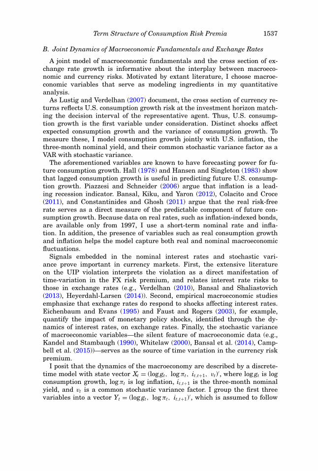
A joint model of macroeconomic fundamentals and the cross section of ex-change rate growth is informative about the interplay between macroeco-nomic and currency risks. Motivated by extant literature, I choose macroe-conomic variables that serve as modeling ingredients in my quantitativeanalysis.
As Lustig and Verdelhan (2007) document, the cross section of currency re-turns reflects U.S. consumption growth risk at the investment horizon match-ing the decision interval of the representative agent. Thus, U.S. consump-tion growth is the first variable under consideration. Distinct shocks affectexpected consumption growth and the variance of consumption growth. Tomeasure these, I model consumption growth jointly with U.S. inflation, thethree-month nominal yield, and their common stochastic variance factor as aVAR with stochastic variance.
The aforementioned variables are known to have forecasting power for fu-ture consumption growth. Hall (1978) and Hansen and Singleton (1983) showthat lagged consumption growth is useful in predicting future U.S. consump-tion growth. Piazzesi and Schneider (2006) argue that inflation is a lead-ing recession indicator. Bansal, Kiku, and Yaron (2012), Colacito and Croce(2011), and Constantinides and Ghosh (2011) argue that the real risk-freerate serves as a direct measure of the predictable component of future con-sumption growth. Because data on real rates, such as inflation-indexed bonds,are available only from 1997, I use a short-term nominal rate and infla-tion. In addition, the presence of variables such as real consumption growthand inflation helps the model capture both real and nominal macroeconomicfluctuations.
Signals embedded in the nominal interest rates and stochastic vari-ance prove important in currency markets. First, the extensive literatureon the UIP violation interprets the violation as a direct manifestation oftime-variation in the FX risk premium, and relates interest rate risks tothose in exchange rates (e.g., Verdelhan (2010), Bansal and Shaliastovich(2013), Heyerdahl-Larsen (2014)). Second, empirical macroeconomic studiesemphasize that exchange rates do respond to shocks affecting interest rates.Eichenbaum and Evans (1995) and Faust and Rogers (2003), for example,quantify the impact of monetary policy shocks, identified through the dy-namics of interest rates, on exchange rates. Finally, the stochastic varianceof macroeconomic variables—the silent feature of macroeconomic data (e.g.,Kandel and Stambaugh (1990), Whitelaw (2000), Bansal et al. (2014), Camp-bell et al. (2015))—serves as the source of time variation in the currency riskpremium.
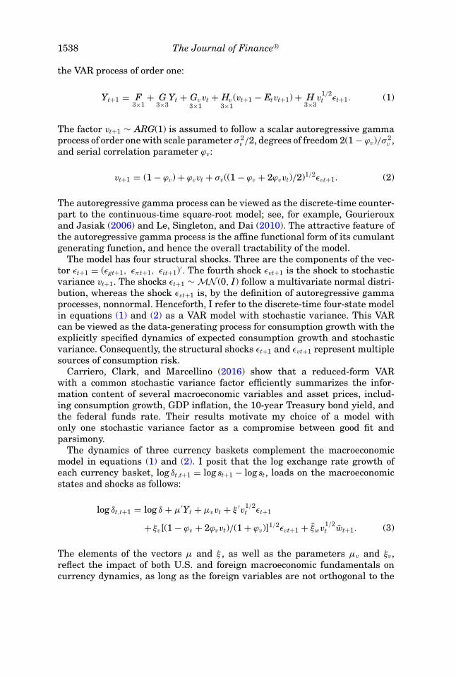
I posit that the dynamics of the macroeconomy are described by a discrete-time model with state vector Xt = (log gt, log πt, it,t+1, vt)′, where log gt is logconsumption growth, log πt is log inflation, it,t+1 is the three-month nominalyield, and vt is a common stochastic variance factor. I group the first threevariables into a vector Yt = (log gt, log πt, it,t+1)′, which is assumed to follow
1538 The Journal of Finance R©
the VAR process of order one:
Yt+1 = F3×1
+ G3×3
Yt + Gv3×1
vt + Hv3×1
(vt+1 − Etvt+1) + H3×3
v1/2t εt+1. (1)
The factor vt+1 ∼ ARG(1) is assumed to follow a scalar autoregressive gammaprocess of order one with scale parameter σ 2
v /2, degrees of freedom 2(1 − ϕv)/σ 2v ,
and serial correlation parameter ϕv:
vt+1 = (1 − ϕv) + ϕvvt + σv((1 − ϕv + 2ϕvvt)/2)1/2εvt+1. (2)
The autoregressive gamma process can be viewed as the discrete-time counter-part to the continuous-time square-root model; see, for example, Gourierouxand Jasiak (2006) and Le, Singleton, and Dai (2010). The attractive feature ofthe autoregressive gamma process is the affine functional form of its cumulantgenerating function, and hence the overall tractability of the model.
The model has four structural shocks. Three are the components of the vec-tor εt+1 = (εgt+1, επt+1, εit+1)′. The fourth shock εvt+1 is the shock to stochasticvariance vt+1. The shocks εt+1 ∼ MN (0, I) follow a multivariate normal distri-bution, whereas the shock εvt+1 is, by the definition of autoregressive gammaprocesses, nonnormal. Henceforth, I refer to the discrete-time four-state modelin equations (1) and (2) as a VAR model with stochastic variance. This VARcan be viewed as the data-generating process for consumption growth with theexplicitly specified dynamics of expected consumption growth and stochasticvariance. Consequently, the structural shocks εt+1 and εvt+1 represent multiplesources of consumption risk.
Carriero, Clark, and Marcellino (2016) show that a reduced-form VARwith a common stochastic variance factor efficiently summarizes the infor-mation content of several macroeconomic variables and asset prices, includ-ing consumption growth, GDP inflation, the 10-year Treasury bond yield, andthe federal funds rate. Their results motivate my choice of a model withonly one stochastic variance factor as a compromise between good fit andparsimony.
The dynamics of three currency baskets complement the macroeconomicmodel in equations (1) and (2). I posit that the log exchange rate growth ofeach currency basket, log δt,t+1 = log st+1 − log st, loads on the macroeconomicstates and shocks as follows:
log δt,t+1 = log δ + μ′Yt + μvvt + ξ ′v1/2t εt+1
+ ξv[(1 − ϕv + 2ϕvvt)/(1 + ϕv)]1/2εvt+1 + ξwv1/2t wt+1. (3)
The elements of the vectors μ and ξ , as well as the parameters μv and ξv,reflect the impact of both U.S. and foreign macroeconomic fundamentals oncurrency dynamics, as long as the foreign variables are not orthogonal to the
Term Structure of Consumption Risk Premia 1539
Table IIDescriptive Statistics
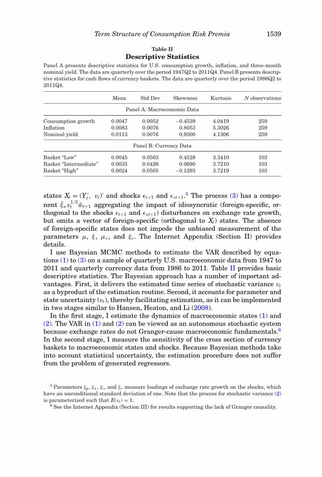
Panel A presents descriptive statistics for U.S. consumption growth, inflation, and three-monthnominal yield. The data are quarterly over the period 1947Q2 to 2011Q4. Panel B presents descrip-tive statistics for cash flows of currency baskets. The data are quarterly over the period 1986Q2 to2011Q4.
Mean Std Dev Skewness Kurtosis N observations
Panel A: Macroeconomic Data
Consumption growth 0.0047 0.0052 −0.4539 4.0419 259Inflation 0.0083 0.0076 0.8053 5.3026 259Nominal yield 0.0113 0.0076 0.9300 4.1306 259
Panel B: Currency Data
Basket “Low” 0.0045 0.0503 0.4528 3.3410 103Basket “Intermediate” 0.0035 0.0426 0.0690 3.7210 103Basket “High” 0.0024 0.0505 −0.1293 3.7219 103
states Xt = (Y ′t , vt)′ and shocks εt+1 and εvt+1.5 The process (3) has a compo-
nent ξwv1/2t wt+1 aggregating the impact of idiosyncratic (foreign-specific, or-
thogonal to the shocks εt+1 and εvt+1) disturbances on exchange rate growth,but omits a vector of foreign-specific (orthogonal to Xt) states. The absenceof foreign-specific states does not impede the unbiased measurement of theparameters μ, ξ , μv, and ξv. The Internet Appendix (Section II) providesdetails.
I use Bayesian MCMC methods to estimate the VAR described by equa-tions (1) to (3) on a sample of quarterly U.S. macroeconomic data from 1947 to2011 and quarterly currency data from 1986 to 2011. Table II provides basicdescriptive statistics. The Bayesian approach has a number of important ad-vantages. First, it delivers the estimated time series of stochastic variance vtas a byproduct of the estimation routine. Second, it accounts for parameter andstate uncertainty (vt), thereby facilitating estimation, as it can be implementedin two stages similar to Hansen, Heaton, and Li (2008).
In the first stage, I estimate the dynamics of macroeconomic states (1) and(2). The VAR in (1) and (2) can be viewed as an autonomous stochastic systembecause exchange rates do not Granger-cause macroeconomic fundamentals.6
In the second stage, I measure the sensitivity of the cross section of currencybaskets to macroeconomic states and shocks. Because Bayesian methods takeinto account statistical uncertainty, the estimation procedure does not sufferfrom the problem of generated regressors.
5 Parameters ξg, ξπ , ξi , and ξv measure loadings of exchange rate growth on the shocks, whichhave an unconditional standard deviation of one. Note that the process for stochastic variance (2)is parameterized such that E(vt) = 1.
6 See the Internet Appendix (Section III) for results supporting the lack of Granger causality.
1540 The Journal of Finance R©
As a part of the estimation output, I obtain the parameter estimates of thecovariance matrix = HH′ and recover disturbances wt+1 ∼ MN (0, I) thatare unknown linear functions of the structural shocks εt+1 ∼ MN (0, I):
Hεt+1 = 1/2wt+1. (4)
The unknown part in the linear mapping (4) is the matrix H. I therefore aug-ment the VAR with a number of identifying restrictions and use methods ofstructural macroeconometrics to estimate the matrix H and recover the struc-tural shocks. I use contemporaneous zero restrictions and consider one of theglobally just-identified systems (Rubio-Ramirez, Waggoner, and Zha (2010)):H13 = H21 = H23 = 0. The results highlighted later in the section are robust tousing alternative shock-identifying assumptions within a class of globally just-identified systems. I label the shocks according to the processes from whichthey originate: consumption growth shock, inflation shock, interest rate shock,and variance shock.
The structural shocks identified from the U.S. data are not necessarily spe-cific to the U.S. economy. Aggregate consumption of any country is an equilib-rium outcome of risk-sharing through trade in goods and asset markets andtherefore reflects both local and global shocks. The relative importance of globalshocks varies across countries. Lustig, Roussanov, and Verdelhan (2011) andVerdelhan (forthcoming) suggest that the global sources of risk must lie atthe core of currency carry trade profitability. Because of the special role of theU.S. economy in the world financial system and trade (e.g., Maggiori (2013)),it is natural to expect that U.S. data are the most informative about globalmacroeconomic disturbances.
C. Cross Section of Multiperiod Currency Risk Exposures
I study the relative importance of the multiple sources of macroeconomicrisk in the FX market in the cross section and at alternative investmenthorizons. It is customary in the literature to measure the quantitative roleof each individual shock by its contribution to the risk premium. The riskpremium depends on two characteristics of a shock: the quantity and theprice of risk. Thus, in the context of my study, the most important shocksare expected to be associated with large economic differences in risk expo-sures across currency baskets and high prices of risk, at multiple investmenthorizons.
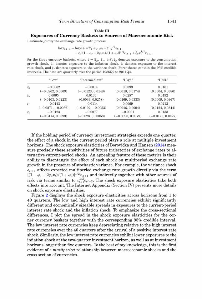
Table III shows that, at the horizon of one quarter, currencies belongingto different interest rate environments load differently on interest rate andinflation shocks. High interest rate currencies appreciate, whereas low in-terest rate currencies depreciate, upon the realization of a positive interestrate shock or inflation shock. This evidence complements the finding of Lustigand Verdelhan (2007), who show that at the one-period investment horizonthere is cross-sectional variation in currency exposures to realized consumptiongrowth.
Term Structure of Consumption Risk Premia 1541
Table IIIExposures of Currency Baskets to Sources of Macroeconomic Risk
I estimate jointly the exchange rate growth process
log δt,t+1 = log δ + μ′Yt + μvvt + ξ ′v1/2t εt+1
+ ξv[(1 − ϕv + 2ϕvvt)/(1 + ϕv)]1/2εvt+1 + ξwv1/2t wt+1
for the three currency baskets, where ξ = (ξg, ξπ , ξi)′; ξg denotes exposure to the consumptiongrowth shock, ξπ denotes exposure to the inflation shock, ξi denotes exposure to the interestrate shock, and ξv denotes exposure to the variance shock. Parentheses contain the 95% credibleintervals. The data are quarterly over the period 1986Q2 to 2011Q4.
“Low” “Intermediate” “High” “HML”
ξg −0.0062 −0.0014 0.0099 0.0161(−0.0262, 0.0069) (−0.0123, 0.0148) (0.0018, 0.0174) (0.0004, 0.0386)
ξπ 0.0065 0.0136 0.0257 0.0192(−0.0103, 0.0223) (0.0036, 0.0258) (0.0169, 0.0333) (0.0009, 0.0367)
ξi −0.0143 −0.0114 0.0069 0.0213(−0.0271, −0.0056) (−0.0192, −0.0053) (0.0046, 0.0094) (0.0124, 0.0344)
ξv −0.0123 −0.0077 −0.0001 0.0133(−0.0414, 0.0093) (−0.0281, 0.0058) (−0.0090, 0.0079) (−0.0120, 0.0427)
If the holding period of currency investment strategies exceeds one quarter,the effect of a shock in the current period plays a role at multiple investmenthorizons. The shock exposure elasticities of Borovicka and Hansen (2014) mea-sure precisely these sensitivities of future trajectories of exchange rates to al-ternative current-period shocks. An appealing feature of these metrics is theirability to disentangle the effect of each shock on multiperiod exchange rategrowth in the presence of stochastic variance. For example, the variance shockεvt+1 affects expected multiperiod exchange rate growth directly via the term[(1 − ϕv + 2ϕvvt)/(1 + ϕv)]1/2εvt+1 and indirectly together with other sources ofrisk via terms similar to v
1/2t+1εgt+2. The shock exposure elasticities take both
effects into account. The Internet Appendix (Section IV) presents more detailson shock exposure elasticities.
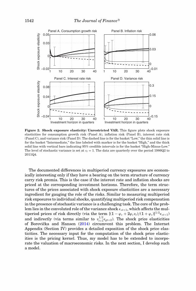
Figure 2 displays the shock exposure elasticities across horizons from 1 to40 quarters. The low and high interest rate currencies exhibit significantlydifferent and economically sizeable spreads in exposures to the current-periodinterest rate shock and the inflation shock. To emphasize the cross-sectionaldifferences, I plot the spread in the shock exposure elasticities for the cor-ner currency baskets together with the corresponding 95% credible interval.The low interest rate currencies keep depreciating relative to the high interestrate currencies over the 40 quarters after the arrival of a positive interest rateshock. Similarly, the low interest rate currencies exhibit lower exposures to theinflation shock at the two-quarter investment horizon, as well as at investmenthorizons longer than five quarters. To the best of my knowledge, this is the firstevidence of a multiperiod relationship between macroeconomic shocks and thecross section of currencies.
1542 The Journal of Finance R©
1 10 20 30 40−0.03
0
0.03
0.05S
hock
exp
osur
e el
astic
ity
Panel A. Consumption growth risk
1 10 20 30 40−0.01
0
0.03
0.06Panel B. Inflation risk
1 10 20 30 40−0.04
0
0.04
0.08
Investment horizon in quarters
Sho
ck e
xpos
ure
elas
ticity
Panel C. Interest rate risk
1 10 20 30 40Investment horizon in quarters
−0.15
0
0.15
0.3
Panel D. Variance risk
Figure 2. Shock exposure elasticity: Unrestricted VAR. This figure plots shock exposureelasticities for consumption growth risk (Panel A), inflation risk (Panel B), interest rate risk(Panel C), and variance risk (Panel D). The dashed line is for the basket “Low,” the thin solid line isfor the basket “Intermediate,” the line labeled with marker is for the basket “High,” and the thicksolid line with vertical bars indicating 95% credible intervals is for the basket “High-Minus-Low.”The level of stochastic variance is set at vt = 1. The data are quarterly over the period 1986Q2 to2011Q4.
The documented differences in multiperiod currency exposures are econom-ically interesting only if they have a bearing on the term structure of currencycarry risk premia. This is the case if the interest rate and inflation shocks arepriced at the corresponding investment horizons. Therefore, the term struc-tures of the prices associated with shock exposure elasticities are a necessaryingredient for gauging the role of the risks. Similar to measuring multiperiodrisk exposures to individual shocks, quantifying multiperiod risk compensationin the presence of stochastic variance is a challenging task. The core of the prob-lem lies in the convoluted role of the variance shock εvt+1, which affects the mul-tiperiod prices of risk directly (via the term [(1 − ϕv + 2ϕvvt)/(1 + ϕv)]1/2εvt+1)and indirectly (via terms similar to v
1/2t+1εgt+2). The shock price elasticities
of Borovicka and Hansen (2014) circumvent this problem. The InternetAppendix (Section IV) provides a detailed exposition of the shock price elas-ticities. The necessary input for the computation of the shock price elastic-ities is the pricing kernel. Thus, my model has to be extended to incorpo-rate the valuation of macroeconomic risks. In the next section, I develop sucha model.
Term Structure of Consumption Risk Premia 1543
II. A Structural Model
This section advances the analysis along two important dimensions. First,it develops an equilibrium framework for studying how the term structure ofcurrency returns reflects the sources of macroeconomic risk. Second, it char-acterizes the properties of the proposed model and discusses the estimationmethodology.
A. The Pricing Kernel
In the context of my analysis, a natural way to characterize compensationfor currency exposures to the multiple sources of macroeconomic risk across al-ternative investment horizons is to develop a consumption-based model with arepresentative agent exhibiting recursive preferences. First, the VAR in equa-tions (1) and (2) can be directly interpreted as a data-generating process forconsumption growth. It has features that are standard in the macro-based as-set pricing literature: time-varying expected consumption growth and stochas-tic variance. Next, the representative agent exhibiting recursive preferences(Kreps and Porteus (1978), Epstein and Zin (1989), Weil (1990)) is averse to anysource of consumption risk, namely, shocks that affect consumption growth con-temporaneously or with a lag of one period, or shocks that drive the stochasticvariance of consumption growth. Therefore, all sources of risk are associatedwith potentially meaningful prices of risk and play a role in asset markets.Henceforth, I use the terms “multiple sources of macroeconomic risk” and “mul-tiple sources of consumption risk” interchangeably.
Taking the above path, the representative agent is endowed with recursiveutility
Ut = [(1 − β)cρ
t + βμt(Ut+1)ρ]1/ρ
, (5)
with certainty equivalent function
μt(Ut+1) = [Et
(U α
t+1
)]1/α, (6)
where ct is consumption at time t, Ut is utility from time t onward, (1 − α) is thecoefficient of relative risk aversion, 1/(1 − ρ) is the elasticity of intertemporalsubstitution (EIS), and β is the subjective discount factor. These preferences,combined with the dynamics of consumption growth described in equations (1)and (2), imply the dynamics of the pricing kernel
log mt,t+1 = log m+ η′Yt + ηvvt + q′v1/2t εt+1
+ qv[(1 − ϕv + 2ϕvvt)/(1 + ϕv)]1/2εvt+1, (7)
where η = (ηg, ηπ , ηi)′ and q = (qg, qπ , qi)′.7 The pricing kernel depends onall of the macroeconomic states Xt = (log gt, log πt, it,t+1, vt)′, one of which,
7 To derive the closed-form solution of the log pricing kernel, I use a log-linear approximation ofthe constant of elasticity substitution recursion (5). The components of the vectors η and q, as well

1544 The Journal of Finance R©
it,t+1, is a transformed asset price. The dual role of the nominal yield, as animplication and a state of the model, translates into a number of cross-equationrestrictions on the parameters of the consumption growth process. Thus, thevaluation exercise requires that a number of cross-equation restrictions thatguarantee internal consistency of the model complement the VAR described byequations (1) and (2).
The parameter restrictions are encoded into the equilibrium relationshipbetween the nominal yield and the states of the model:8
it,t+1 ≡ Alog gt + Blog πt + Cit,t+1 + Dvt + E, (8)
where A, B, C, D, and E are functions of the preference parameters and struc-tural parameters of the consumption growth process (see Appendix B ). Identity(8) holds if
A = B = D = E = 0,
C = 1.
The restrictions A = B = 0 and C = 1 are linear and can be represented as
G21
G11= G22
G12= G23 − 1
G13= ρ − 1. (9)
The restriction E = 0,
E = − log m+ e′2 F + (1 − ϕv) log (1 − σ 2
v (qv − e′2 Hv)/2)
σ 2v /2
+ (qv − e′2 Hv)(1 − ϕv)
is nonlinear, but can be approximated to the linear restriction
− log β + e′2 F − (ρ − 1)e′
1 F = 0 (10)
by applying the first-order Taylor expansion to the logarithmic function. Theapproximation is accurate as it does not distort the pricing implications of themodel.
The nonlinear restriction D = 0,
− (ηv − e′
2Gv
) − 12
(q′ − e′
2 H) (
q′ − e′2 H
)′ + ϕv
(qv − e′
2 Hv
)
− ϕv(qv − e′2 Hv)
1 − σ 2v (qv − e′
2 Hv)/2= 0 (11)
as a function of the endogenous parameters of the utility recursion, does nothave an accurate linear approximation. As a result, estimation of the consump-tion growth process in equations (1) and (2) together with the cross-equation
as the parameters ηv and qv , are functions of the structural parameters of the model. Appendix Bprovides corresponding details.
8 The nominal pricing kernel, necessary to derive the nominal yield, is obtained by subtractinginflation given by (1) and (2) from the real pricing kernel (7).

Term Structure of Consumption Risk Premia 1545
restrictions (9) to (11) is challenging due to the featured nonlinearity. However,the nonlinear restriction plays a central role in the subsequent analysis: in itsabsence, the pricing implications of the model are severely biased. The InternetAppendix (Section V) discusses the role of the cross-equation restrictions forthe prices of risk.
B. Empirical Approach
As in Section II, I use Bayesian MCMC methods to estimate a VAR of macroe-conomic variables and exchange rates that I interpret as a joint model ofconsumption growth and a cross section of currency baskets. The importantdifference relative to the prior VAR is the imposition of the cross-equationrestrictions (9) to (11) on the parameters of the data-generating process forconsumption growth. The challenge lies in the presence of the nonlinear re-striction (11). The Bayesian methods allow one to accommodate the nonlinearparameter restriction directly by rejecting parameter draws that violate theparameter constraint.
At the estimation stage, I account for regularity conditions, ensuring thatthe nonlinear forward-looking difference equation defining the recursive util-ity has a unique solution, and shock exposure and shock price elasticities aredefined at an infinite investment horizon. To derive the corresponding param-eter restrictions, I follow Hansen and Scheinkman (2009, 2012). The InternetAppendix (Section VI) contains the relevant details.
The cross-equation restrictions (9) to (11) are functions of the 22 structuralparameters governing the dynamics of the VAR with stochastic variance andthe preference parameters α, β, and ρ. I estimate the elements of the matricesF, G, Gv, Hv, and , as well as the parameters of the stochastic variance ϕv
and σ 2v , and I calibrate the preference parameters α = −9, β = 0.9924, and
ρ = 1/3.9 The values of the preference parameters α and ρ imply a preferencefor the early resolution of uncertainty and have been extensively used in theliterature to address a number of asset pricing puzzles. For example, by usingthese preference parameters, Bansal and Yaron (2004) explain salient featuresof the equity market in an equilibrium endowment economy, Hansen, Heaton,and Li (2008) empirically explain the value premium puzzle, and Bansal andShaliastovich (2013) rationalize properties of the term structure of nominalinterest rates and the violation of UIP. In addition, in the international settingColacito and Croce (2013) argue that EIS = 3/2 (ρ = 1/3) is supported by em-pirical evidence obtained through the lens of their structural model. The valueof the subjective discount factor β comes from Hansen, Heaton, and Li (2008).
9 The long-run risk literature traditionally uses monthly calibrations with a risk aversion of 10and an EIS of 1.5, whereas I use quarterly data for estimation. Hansen, Heaton, and Li (2008)also use quarterly consumption data to identify the short-run and permanent consumption shocks,and assume similar preference parameters to price assets. Importantly, however, these preferenceparameters are, if anything, conservative at lower frequencies. See Bansal, Kiku, and Yaron (2012)for a related discussion of how a model specified at a lower frequency pushes an estimate for theparameter of risk aversion upward.

1546 The Journal of Finance R©
I identify structural shocks εt+1 from the reduced-form innovations wt+1, asis common in structural VARs in applied macroeconomics. Because preferencesaugment the model of consumption growth, important economic considerationslead to a limited choice of identification schemes compared to the case of thereduced-form analysis of Section II. Specifically, economic intuition suggeststhat only two of six globally just-identified systems with contemporaneous zerorestrictions make sense. The identifications are labeled “Fast Consumption”and “Fast Inflation” and differ in terms of the identifying assumptions aboutshocks εgt+1 and επt+1. I borrow the terminology of “fast variables” from struc-tural VARs in applied macroeconomics. The Internet Appendix (Section VII)explains the motivation for the choice of identifying restrictions.
Under “Fast Consumption” (“Inflation”), consumption growth (inflation) re-acts contemporaneously to an inflation (consumption growth) shock, whereasinflation (consumption growth) reacts to a consumption growth (inflation)shock with a one-quarter delay. Henceforth, I focus my analysis on the caseof “Fast Consumption” identification; H13 = H21 = H23 = 0. The Internet Ap-pendix (Section VIII) contains details related to “Fast Inflation” identification.The results are qualitatively robust across identification schemes. The quanti-tative difference comes from differences in the prices of risk for the consumptiongrowth and inflation shocks.
A detailed discussion of the remaining technical issues associated withthe empirical implementation appears in the Internet Appendix. Specifically,Section VII contains the estimation algorithm and reports the choice of priors. Italso explains how pricing restrictions are imposed and how structural shocksare identified. Finally, it explains why preference parameters are calibratedrather than estimated.
III. Results
In this section, I analyze how multiple sources of consumption risk are re-flected in the cross section of currency returns at multiple investment horizonsthrough the lens of the structural consumption-based model of a representa-tive agent with recursive preferences. Armed with the estimated dynamics ofthe pricing kernel, I describe how featured multiperiod currency risk expo-sures are priced in the marketplace. I then aggregate information encoded inthe term structures of currency exposures and prices of risk to identify themost important sources of currency risk. Next, I analyze empirical propertiesof these shocks as they relate to the distribution of consumption growth. I con-clude by suggesting economic channels of risk propagation consistent with thedocumented empirical facts.
A. Term Structure of Consumption Risk Premia in the Cross Sectionof Currency Returns
The quantitative importance of alternative sources of risk in asset mar-kets is traditionally measured by the size of the risk premium earned as
Term Structure of Consumption Risk Premia 1547
compensation for assets’ risk exposures to the shocks. Two components of riskpremium matter: the quantity and the price of risk. These two characteristicsvary across assets and investment horizons. A natural consequence of this is thecross-sectional variation in risk premia, potentially across many investmenthorizons.
The term structure of average carry log returns depicted in Figure 1 is adirect manifestation of the cross-sectional variation in currency risk premiaat many investment horizons. To determine which sources of consumption riskare reflected in carry risk premia, I analyze the interaction between the shocks,identified from the structural VAR, and currency baskets according to the fol-lowing quantitative criteria.10 A source of consumption risk is reflected in theterm structure of carry risk premia if (i) currency baskets exhibit statisticallydifferent and economically sizeable exposures to the shock at many investmenthorizons and (ii) the prices of the corresponding risk exposures are economicallymeaningful and statistically significant.
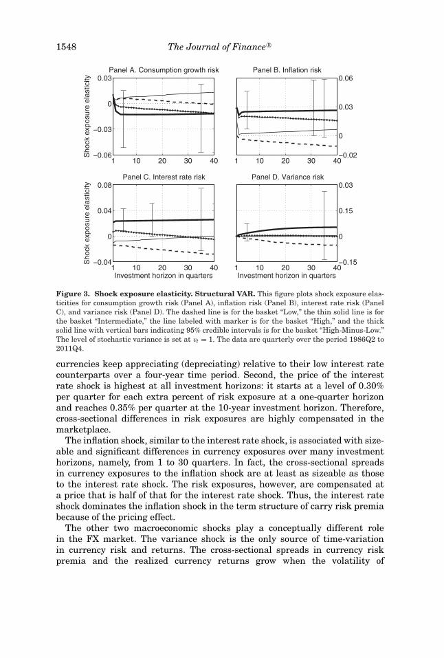
Figure 3 displays shock exposure elasticities, that is, the sensitivities of cur-rency baskets to the multiple sources of consumption risk, across investmenthorizons from one quarter up to 10 years. This is a counterpart to Figure 2 in mystructural model. To highlight the cross-sectional differences, I plot the spreadin the shock exposure elasticities for the corner currency baskets together withthe corresponding 95% credible interval. Figure 4 displays shock price elas-ticities, that is, multiperiod compensation for the corresponding currency risksensitivities, across the same investment horizons. The shock price elastici-ties of the variance shock are basket-specific. To compare the marginal pricesof the variance risk, I plot the difference in the prices for the corner basketstogether with the corresponding 95% credible interval. The shock elasticitiesscale up or down depending on the magnitude of the stochastic variance. In thefigures, I set vt at its long-run mean value of one. At times of high macroeco-nomic volatility, the shock exposure elasticities become more cross-sectionallydisperse, whereas the shock price elasticities increase. Naturally, these cyclicalproperties have direct consequences for the business cycle variation in currencyrisk premia that I analyze later in this section.
An analysis of shock elasticities confirms the dominant role of interest rateshock that was uncovered in the structural VAR. The properties of inter-est rate risk satisfy the two aforementioned criteria of quantitative promi-nence. First, higher yield currencies exhibit significantly higher exposuresto the interest rate shock at horizons from 1 to 16 quarters.11 Thus, upontoday’s realization of a positive (negative) interest rate shock, high-yield
10 Appendix D contains an estimation output of the VAR in (1) to (3) with cross-equation re-strictions (9) to (11). The Internet Appendix (Section VII) discusses the properties of the estimateddynamics of consumption growth.
11 The shapes of the shock elasticities change in the presence of cross-equation restrictions.Nevertheless, the shock exposure elasticities implied by the unrestricted VAR in (1) and (2) and itsconstrained counterpart, augmented with cross-equation restrictions (9) to (11), are statisticallyindistinguishable from each other (Figure C.1). I interpret this as evidence suggesting that datafail to reject the structural restrictions.
1548 The Journal of Finance R©
1 10 20 30 40−0.06
−0.03
0
0.03S
hock
exp
osur
e el
astic
ity
Panel A. Consumption growth risk
1 10 20 30 40−0.02
0
0.03
0.06Panel B. Inflation risk
1 10 20 30 40−0.04
0
0.04
0.08
Sho
ck e
xpos
ure
elas
ticity
Investment horizon in quarters
Panel C. Interest rate risk
1 10 20 30 40Investment horizon in quarters
−0.15
0
0.15
0.03Panel D. Variance risk
Figure 3. Shock exposure elasticity. Structural VAR. This figure plots shock exposure elas-ticities for consumption growth risk (Panel A), inflation risk (Panel B), interest rate risk (PanelC), and variance risk (Panel D). The dashed line is for the basket “Low,” the thin solid line is forthe basket “Intermediate,” the line labeled with marker is for the basket “High,” and the thicksolid line with vertical bars indicating 95% credible intervals is for the basket “High-Minus-Low.”The level of stochastic variance is set at vt = 1. The data are quarterly over the period 1986Q2 to2011Q4.
currencies keep appreciating (depreciating) relative to their low interest ratecounterparts over a four-year time period. Second, the price of the interestrate shock is highest at all investment horizons: it starts at a level of 0.30%per quarter for each extra percent of risk exposure at a one-quarter horizonand reaches 0.35% per quarter at the 10-year investment horizon. Therefore,cross-sectional differences in risk exposures are highly compensated in themarketplace.
The inflation shock, similar to the interest rate shock, is associated with size-able and significant differences in currency exposures over many investmenthorizons, namely, from 1 to 30 quarters. In fact, the cross-sectional spreadsin currency exposures to the inflation shock are at least as sizeable as thoseto the interest rate shock. The risk exposures, however, are compensated ata price that is half of that for the interest rate shock. Thus, the interest rateshock dominates the inflation shock in the term structure of carry risk premiabecause of the pricing effect.
The other two macroeconomic shocks play a conceptually different rolein the FX market. The variance shock is the only source of time-variationin currency risk and returns. The cross-sectional spreads in currency riskpremia and the realized currency returns grow when the volatility of

Term Structure of Consumption Risk Premia 1549
1 10 20 30 40−0.1
0
0.2
0.4S
hock
pric
e el
astic
ity
Panel A. Consumption growth risk
1 10 20 30 40−0.1
0
0.2
0.4
Panel B. Inflation risk
1 10 20 30 40−0.1
0
0.2
0.4
Sho
ck p
rice
elas
ticity
Investment horizon in quarters
Panel C. Interest rate risk
1 10 20 30 40Investment horizon in quarters
−0.1
0
0.2
0.4
Panel D. Variance risk
Figure 4. Shock price elasticity. This figure plots shock price elasticities for consumptiongrowth risk (Panel A), inflation risk (Panel B), interest rate risk (Panel C), and variance risk(Panel D). In Panels A, B, and C shock price elasticity is the same for the currency baskets. InPanel D, shock price elasticity is basket specific. The dashed line is for the basket “Low,” the thinsolid line is for the basket “Intermediate,” the line labeled with marker is for the basket “High,”and the thick solid line with vertical bars indicating 95% credible intervals is for the basket “High-Minus-Low.” The level of stochastic variance is set at vt = 1. The data are quarterly over the period1986Q2 to 2011Q4.
macroeconomic shocks is high and decline when volatility is low. The con-sumption growth shock matters only for high-yield currencies: shock expo-sure elasticities are positive and significant at the one-quarter investmenthorizon.
Having established how currencies from different interest rate environmentsare exposed to the multiple sources of macroeconomic risk across alternativeinvestment horizons and how these risk exposures are priced, the next step isto aggregate this information and deduce implications for the term structure ofcarry risk premia. An important open question is whether total compensationfor exposures of carry portfolio to the multiple sources of consumption riskmatches the level and shape of the term structure of carry returns.
Figure 1 shows that at horizons from 1 to 10 quarters, the carry risk premiaare positive, economically sizeable, and significant. In normal times, that is,when macroeconomic variance is at its long-run mean of one, the risk pre-mium reaches 1.31% per quarter. The risk premium is rather flat but be-comes insignificant at horizons longer than 10 quarters. Overall, the model-implied term structure of carry risk premia matches closely the shape and

1550 The Journal of Finance R©
Table IVOne-Period Risk Premium Decomposition
This table presents the decomposition of the three-month currency risk premia into contributionsof multiple sources of risk. εgt+1 denotes consumption growth risk, επt+1 denotes inflation risk,εit+1 denotes interest rate risk, and εvt+1 denotes variance risk. The level of stochastic variance isset at vt = 1. Parentheses contain the 95% credible intervals. The row “Data” contains descriptivestatistics for one-period average carry log returns. Brackets contain standard errors. The data arequarterly over the period 1986Q2 to 2011Q4. Numbers are in percent.
“Low” “Intermediate” “High” “HML”
εgt+1 0.0392 0.2156 0.2442 0.2051(−0.5817, 0.8878) (−0.1872, 0.4515) (0.1264, 0.3905) (−0.6659, 0.8925)
επt+1 −0.0053 0.2243 0.4239 0.4292(−0.3597, 0.2164) (−0.0142, 0.4515) (0.2420, 0.6315) (0.1745, 0.8018)
εit+1 −0.4398 −0.3603 0.2082 0.6480(−0.9264, −0.0435) (−0.7932, −0.1002) (0.1198, 0.3084) (0.2541, 1.1353)
εvt+1 −0.0263 −0.0041 0.0006 0.0269(−0.3661, 0.2747) (−0.2392, 0.2384) (−0.2216, 0.2046) (−0.3262, 0.4164)
Total −0.4322 0.0755 0.8769 1.3091(−0.9030, −0.0115) (−0.3817, 0.5042) (0.5312, 1.1939) (0.8231, 1.8087)
Data 0.0826 0.5355 1.2120 1.1294[0.5063] [0.4279] [0.4996] [0.4416]
level of the term structure of average carry returns in the data.12 This descrip-tion of the multiperiod carry risk premia is complementary to that of Lustig,Stathopoulos, and Verdelhan (2016), who characterize the term structure ofone-period risk premia obtainable as a result of investing in foreign bonds ofvarious maturities.
It is customary in asset pricing to measure the role of alternative sources ofrisk by their corresponding contributions to the total risk premium. In the pres-ence of stochastic variance, measuring multiperiod risk premia attributableto shocks of different types is methodologically challenging. The core of theproblem lies in the convoluted role of the current-period variance shock, whichmultiplicatively interacts with all the future shocks (see Borovicka et al. (2011)for further details). In the face of this challenge, I can only explicitly charac-terize the one-period risk premium decomposition. I rely on shock elasticitiesfor gauging the relative importance of shocks across multiperiod investmenthorizons.
Table IV shows the decomposition of the total one-period carry risk premiuminto contributions attributable to alternative sources of consumption risk. As
12 I measure slightly different objects in the data and in the model. In the data, I measureaverage log returns on carry trade E log rxt,t+τ . In the model, I measure the conditional log riskpremium log Etrxt,t+τ and evaluate it at the unconditional mean of the stochastic variance vt = 1.The difference between these two objects is E log Etrxt,t+τ − E log rxt,t+τ = 1
2 E vart log rxt,t+τ . Icheck that the model counterpart of the expected log return does not differ much from the model-implied risk premium. The dashed black line in Figure 1 displays E log rxt,t+τ implied by themodel.
Term Structure of Consumption Risk Premia 1551
expected from the analysis of shock elasticities, only the interest rate and in-flation shocks are associated with significant risk premia. Their contributionsconstitute 60% and 40% of the total risk premium, respectively. To measurethese relative contributions, I divide the individual risk premia for the interestrate and inflation shocks by the sum of the two, thereby ignoring the insignifi-cant premia associated with the consumption growth and variance shocks.
The variance risk contributes to the currency risk premium in a conceptuallydifferent way. This shock is the only source of business cycle variation in thecurrency risk premia at all investment horizons. During low volatility episodes(vt = 0.33) the one-period carry premium could be as low as 0.43% per quarter,whereas during turbulent times (vt = 2.72) it could be as high as 3.54% perquarter. To report these numbers, I scale the one-period average risk premiaof 1.31% per quarter by the corresponding values of the stochastic variance.The role of the consumption growth shock is limited to high-yield currencies atthe one-period investment horizon: the risk compensation for bearing a three-month exposure of high-yield currencies to the shock is 0.24% per quarter(Table IV). The presence of this risk compensation only at the one-period in-vestment horizon explains the larger currency carry premium at the short endof the term structure.
B. Economic Underpinnings of the FX Risk
The term structure of carry risk premia reflects sources of consumption risk—interest rate and inflation shocks—across multiple investment horizons. Thisnovel empirical fact is encouraging for macro-based models of the risk-returntrade-off in the FX market and complements scarce prior evidence on the inter-play between macroeconomic and currency risk. For earlier contributions, seeCumby (1988), Lustig and Verdelhan (2007), and Sarkissian (2003). To makefurther progress in understanding the currency risk premium, I analyze theproperties of the estimated shocks and suggest economic environments thatcould be consistent with the documented evidence.
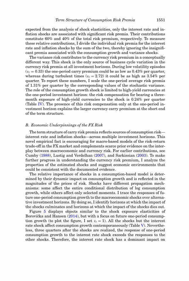
The relative importance of shocks in a consumption-based model is deter-mined by their dynamic impact on consumption growth and is reflected in themagnitudes of the prices of risk. Shocks have different propagation mech-anisms: some affect the entire conditional distribution of log consumptiongrowth, while others affect only selected moments. I trace the responses of fu-ture one-period consumption growth to the macroeconomic shocks over alterna-tive investment horizons. By doing so, I identify horizons at which the impact ofthe shocks culminates and horizons at which the impact of the shocks dies out.
Figure 5 displays objects similar to the shock exposure elasticities ofBorovicka and Hansen (2014), but with a focus on future one-period consump-tion growth (to plot the figure, I set vt = 1). All the shocks but the interestrate shock affect consumption growth contemporaneously (Table V). Neverthe-less, three quarters after the shocks are realized, the response of one-periodconsumption growth to the interest rate shock exceeds the responses to theother shocks. Therefore, the interest rate shock has a dominant impact on
1552 The Journal of Finance R©
5 10 15 20 25 30 35 40−2
0
2
4
6
8
10
12x 10
−3
Dyn
amic
res
pons
e of
exp
ecte
d co
nsum
ptio
n gr
owth
to th
e st
ruct
ural
sho
cks
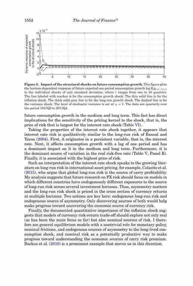
Figure 5. Impact of the structural shocks on future consumption growth. This figure plotsthe horizon-dependent response of future expected one-period consumption growth log Etgt+i−1,t+ito the individual shocks of unit standard deviation, where i ranges from one to 40 quarters.The line labeled with marker is for the consumption growth shock. The thin solid line is for theinflation shock. The thick solid grey line is for the long-run growth shock. The dashed line is forthe variance shock. The level of stochastic variance is set at vt = 1. The data are quarterly overthe period 1947Q2 to 2011Q4.
future consumption growth in the medium and long term. This fact has directimplications for the sensitivity of the pricing kernel to the shock, that is, theprice of risk that is largest for the interest rate shock (Table VI).
Taking the properties of the interest rate shock together, it appears thatinterest rate risk is qualitatively similar to the long-run risk of Bansal andYaron (2004). First, it originates in a persistent variable, that is, the interestrate. Next, it affects consumption growth with a lag of one period and hasa dominant impact on it in the medium and long term. Furthermore, it isthe dominant source of variation in the real risk-free rate (Table V, Panel B).Finally, it is associated with the highest price of risk.
Such an interpretation of the interest rate shock speaks to the growing liter-ature on long-run risk in international asset pricing, for example, Colacito et al.(2015), who argue that global long-run risk is the source of carry profitability.My analysis suggests that future research on FX risk should focus on models inwhich different countries have endogenously different exposures to the sourceof long-run risk across several investment horizons. Thus, asymmetry mattersand the long-run risk shock is priced in the cross section of currency returnsat multiple horizons. Two notions are key here: endogenous long-run risk andendogenous source of asymmetry. Only discovering sources of both would helpmake progress toward uncovering the economic source of currency risk.
Finally, the documented quantitative importance of the inflation shock sug-gests that models of currency risk-return trade-off should explore not only real(as has been the main focus so far) but also nominal sources of risk. I there-fore see general equilibrium models with a nontrivial role for monetary policy,nominal frictions, and endogenous sources of asymmetry to the long-lived con-sumption shock, and nominal risk as a potentially productive way to makeprogress toward understanding the economic sources of carry risk premium.Backus et al. (2010) is a prominent example that moves us in this direction.
Term Structure of Consumption Risk Premia 1553
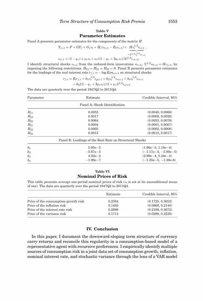
Table VParameter Estimates
Panel A presents parameter estimates for the components of the matrix H
Yt+1 = F + GYt + Gvvt + Hv(vt+1 − Etvt+1) + Hv1/2t εt+1︸ ︷︷ ︸
=1/2v1/2t wt+1
,
vt+1 = (1 − ϕv) + ϕvvt + σv((1 − ϕv + 2ϕvvt)/2)1/2εvt+1.
I identify structural shocks εt+1 from the reduced-form innovations wt+1, 1/2wt+1 = Hεt+1, byimposing the following restrictions: H13 = H21 = H23 = 0. Panel B presents parameter estimatesfor the loadings of the real interest rate r f ,t = − log Etmt,t+1 on structural shocks
r f ,t = Etr f ,t + h1v1/2t εgt+1 + h2v
1/2t επt+1 + h3v
1/2t εit+1
+ h4[(1 − ϕv + 2ϕvvt)/(1 + ϕv)]1/2εvt+1.
The data are quarterly over the period 1947Q2 to 2011Q4.
Parameter Estimate Credible Interval, 95%
Panel A: Shock Identification
H11 0.0055 (0.0046, 0.0066)H12 0.0017 (0.0008, 0.0028)H22 0.0064 (0.0055, 0.0076)H31 0.0004 (0.0001, 0.0007)H32 0.0005 (0.0002, 0.0008)H33 0.0015 (0.0013, 0.0017)
Panel B: Loadings of the Real Rate on Structural Shocks
h1 5.95e−5 (1.66e−5, 1.18e−4)h2 −5.67e−5 (−1.17e−4, −2.00e−5)h3 4.02e−4 (2.99e−4, 5.24e−4)h4 −1.90e−7 (−1.35e−5, −1.39e-6)
Table VINominal Prices of Risk
This table presents average one-period nominal prices of risk (vt is set at its unconditional meanof one). The data are quarterly over the period 1947Q2 to 2011Q4.
Estimate Credible Interval, 95%
Price of the consumption growth risk 0.2384 (0.1725, 0.3052)Price of the inflation risk 0.1483 (0.0868, 0.2140)Price of the interest rate risk 0.2986 (0.2198, 0.3672)Price of the variance risk 0.1714 (0.0299, 0.3238)
IV. Conclusion
In this paper, I document the downward-sloping term structure of currencycarry returns and reconcile this regularity in a consumption-based model of arepresentative agent with recursive preferences. I empirically identify multiplesources of consumption risk in a joint data set of consumption growth, inflation,nominal interest rate, and stochastic variance through the lens of a VAR model
1554 The Journal of Finance R©
with cross-equation restrictions derived under recursive preferences. I findthat higher yield currencies have systematically higher exposures to interestrate and inflation shocks across multiple investment horizons. The currencyexposures are economically meaningfully priced in the marketplace. As a result,the interest rate and inflation shocks are reflected in the term structure of carryrisk premia.
The interest rate shock is qualitatively similar to the long-run risk of Bansaland Yaron (2004): (i) it affects consumption growth with a lag of one quarter,(ii) it exerts a dominant effect on future consumption growth at medium- andlong-term horizons, (iii) it carries the highest price of risk, and (iv) it explainsthe major part of the variation in the real risk-free rate. The inflation shockoperates as a nominal source of risk. The empirical facts documented in thispaper suggest that a potentially productive framework for understanding eco-nomic sources of currency risk is a general equilibrium model with a nontrivialrole for monetary policy, nominal frictions, and endogenous sources of asymme-try to the long-lived consumption shock and nominal risk. I leave it for futureresearch to develop such a framework.
Initial submission: September 16, 2015; Accepted: May 23, 2016Editors: Bruno Biais, Michael R. Roberts, and Kenneth J. Singleton
Appendix A: Data
A. Currency and Interest Rate Data
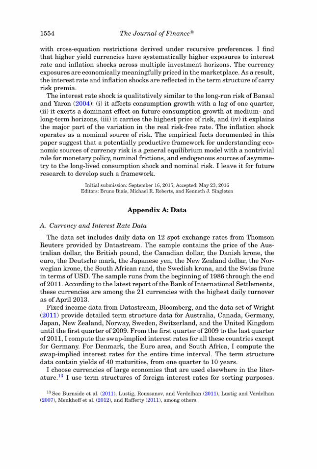
The data set includes daily data on 12 spot exchange rates from ThomsonReuters provided by Datastream. The sample contains the price of the Aus-tralian dollar, the British pound, the Canadian dollar, the Danish krone, theeuro, the Deutsche mark, the Japanese yen, the New Zealand dollar, the Nor-wegian krone, the South African rand, the Swedish krona, and the Swiss francin terms of USD. The sample runs from the beginning of 1986 through the endof 2011. According to the latest report of the Bank of International Settlements,these currencies are among the 21 currencies with the highest daily turnoveras of April 2013.
Fixed income data from Datastream, Bloomberg, and the data set of Wright(2011) provide detailed term structure data for Australia, Canada, Germany,Japan, New Zealand, Norway, Sweden, Switzerland, and the United Kingdomuntil the first quarter of 2009. From the first quarter of 2009 to the last quarterof 2011, I compute the swap-implied interest rates for all these countries exceptfor Germany. For Denmark, the Euro area, and South Africa, I compute theswap-implied interest rates for the entire time interval. The term structuredata contain yields of 40 maturities, from one quarter to 10 years.
I choose currencies of large economies that are used elsewhere in the liter-ature.13 I use term structures of foreign interest rates for sorting purposes.
13 See Burnside et al. (2011), Lustig, Roussanov, and Verdelhan (2011), Lustig and Verdelhan(2007), Menkhoff et al. (2012), and Rafferty (2011), among others.

Term Structure of Consumption Risk Premia 1555
Because of the limited availability of term structure data, my sample containsa smaller number of currencies. I work with quarterly currency quotes sam-pled at the end of the corresponding quarter to match the frequency of theconsumption data.
B. Macro Data
The data set consists of quarterly data on U.S. consumption growth, infla-tion, and three-month nominal yield from the second quarter of 1947 throughthe fourth quarter of 2011. In total, there are 259 observations. The Na-tional Income and Product Accounts (NIPA) tables of the Bureau of Eco-nomic Analysis provide consumption and price data, including table 2.1 (Per-sonal income and its disposition), table 2.3.4 (Personal indexes for personalconsumption expenditures by major type of product), and table 2.3.5 (Per-sonal consumption expenditures by major type of product). Real consump-tion is measured as per capita expenditure on nondurable goods and ser-vices. Nondurable goods and services is the sum of entries from table 2.3.5of row 8 divided by entries from table 2.3.4 of row 8 and components fromtable 2.3.5 of row 13 divided by components from table 2.3.4 of row 13. I con-struct the price index associated with personal consumption expenditures. Row40 of table 2.1 provides population data. The nominal yield comes from CRSP.
Appendix B: Model Solution and Pricing Restrictions
In this appendix, I solve the model. I briefly repeat the main building blocksfor ease of explanation.
The representative agent has recursive preferences
Ut = [(1 − β)cρt + βμt(Ut+1)ρ]1/ρ (B1)
with certainty equivalent function
μt(Ut+1) = [Et(U αt+1)]1/α (B2)
and preference parameters α (risk aversion is 1 − α), β (subjective discountfactor), and ρ (recall that 1/(1 − ρ) is the EIS).
A discrete-time model with four state variables Xt = (log gt, log πt, i′t,t+1, vt)′
describes the consumption growth process. I group the first three variables intovector Yt = (log gt, log πt, it,t+1)′, which follows a VAR process of order one:
Yt+1 = F + GYt + Gvvt + Hv(vt+1 − Etvt+1) + Hv1/2t εt+1. (B3)
The common stochastic variance factor vt+1 ∼ ARG(1) follows a scalar autore-gressive gamma process of order one with scale parameter σ 2
v /2, degrees offreedom 2(1 − ϕv)/σ 2
v , and serial correlation parameter ϕv,
vt+1 = (1 − ϕv) + ϕvvt + σv((1 − ϕv + 2ϕvvt)/2)1/2εvt+1, (B4)
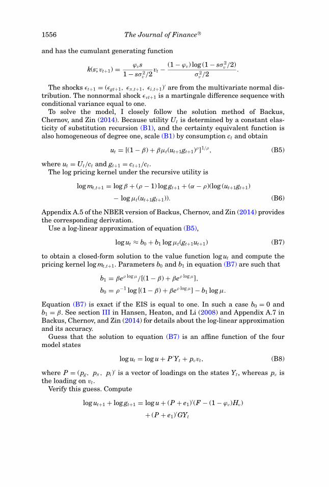
1556 The Journal of Finance R©
and has the cumulant generating function
k(s; vt+1) = ϕvs1 − sσ 2
v /2vt − (1 − ϕv) log (1 − sσ 2
v /2)σ 2
v /2.
The shocks εt+1 = (εgt+1, επ,t+1, εi,t+1)′ are from the multivariate normal dis-tribution. The nonnormal shock εvt+1 is a martingale difference sequence withconditional variance equal to one.
To solve the model, I closely follow the solution method of Backus,Chernov, and Zin (2014). Because utility Ut is determined by a constant elas-ticity of substitution recursion (B1), and the certainty equivalent function isalso homogeneous of degree one, scale (B1) by consumption ct and obtain
ut = [(1 − β) + βμt(ut+1gt+1)ρ]1/ρ, (B5)
where ut = Ut/ct and gt+1 = ct+1/ct.The log pricing kernel under the recursive utility is
log mt,t+1 = log β + (ρ − 1) log gt+1 + (α − ρ)(log (ut+1gt+1)
− log μt(ut+1gt+1)). (B6)
Appendix A.5 of the NBER version of Backus, Chernov, and Zin (2014) providesthe corresponding derivation.
Use a log-linear approximation of equation (B5),
log ut ≈ b0 + b1 log μt(gt+1ut+1) (B7)
to obtain a closed-form solution to the value function log ut and compute thepricing kernel log mt,t+1. Parameters b0 and b1 in equation (B7) are such that
b1 = βeρ log μ/[(1 − β) + βeρ log μ],
b0 = ρ−1 log [(1 − β) + βeρ log μ] − b1 log μ.
Equation (B7) is exact if the EIS is equal to one. In such a case b0 = 0 andb1 = β. See section III in Hansen, Heaton, and Li (2008) and Appendix A.7 inBackus, Chernov, and Zin (2014) for details about the log-linear approximationand its accuracy.
Guess that the solution to equation (B7) is an affine function of the fourmodel states
log ut = log u + P ′Yt + pvvt, (B8)
where P = (pg, pπ , pi)′ is a vector of loadings on the states Yt, whereas pv isthe loading on vt.
Verify this guess. Compute
log ut+1 + log gt+1 = log u + (P + e1)′(F − (1 − ϕv)Hv)
+ (P + e1)′GYt

Term Structure of Consumption Risk Premia 1557
+ (P + e1)′(Gv − ϕv Hv)vt
+ (P + e1)′Hv1/2t εt+1
+ ((P + e1)′Hv + pv)vt+1,
where e1 is a coordinate vector with the first element equal to one.The log of the certainty equivalent function is
log μt(ut+1gt+1) = log u + (P + e1)′(F − (1 − ϕv)Hv) − (1 − ϕv) log (1 − α pvσ2v /2)
ασ 2v /2
+ (P + e1)′GYt + (P + e1)′(Gv − ϕv Hv)vt
+ α
2(P + e1)′(P + e1)vt + ϕv pvvt
1 − α pvσ 2v /2
, (B9)
where pv = (P + e1)′Hv + pv, = HH′. Substitute (B8) and (B9) into equa-tion (B7) and collect and match the corresponding terms. Equation (B7) hasa constant term and four variables, and hence, we obtain the system of fiveequations
log u = b0 + b1 log u + b1(P + e1)′(F − (1 − ϕv)Hv)
− b1(1 − ϕv) log (1 − α pvσ2v /2)
ασ 2v /2
, (B10)
pg = b1(P + e1)′Ge1,
pπ = b1(P + e1)′Ge2,
pi = b1(P + e1)′Ge3,
pv = b1
((P + e1)′(Gv − ϕv Hv) + α
2(P + e1)′(P + e1) + ϕv pv
1 − α pvσ 2v /2
),
where ei (i = 1, 2, 3) are the coordinate vectors with the ith element equal toone.
Equations for pg, pπ , and pi are linear and therefore result in uniquesolutions
pg = Ag/Bg,
pπ = Aπ/Bπ ,
pi = Ai/Bi,
where
Ag = − (G11b1 − G11G22b21 + G12G21b2
1 − G11G33b21 + G13G31b2
1 + G11G22G33b31
− G11G23G32b31 − G12G21G33b3
1 + G12G23G31b31 + G13G21G32b3
1
− G13G22G31b31),
1558 The Journal of Finance R©
Aπ = − (G12b1 + G13G32b21 − G12G33b2
1),
Ai = − (G13b1 + G12G23b21 − G13G22b2
1),
Bg = Bπ = Bi
= G11b1 + G22b1 + G33b1 − G11G22b21 + G12G21b2
1 − G11G33b21 + G13G31b2
1
− G22G33b21 + G23G32b2
1 + G11G22G33b31 − G11G23G32b3
1 − G12G21G33b31
+ G12G23G31b31 + G13G21G32b3
1 − G13G22G31b31 − 1.
The equation for pv is quadratic
Av p2v + Bv pv + Cv = 0,
where
Av = ασ 2v
2,
Bv = b1ϕv − ασ 2v
2Dv − 1 + ασ 2
v
2(P + e1)′Hv,
Cv = Dv
(1 − ασ 2
v
2(P + e1)′Hv
)+ b1ϕv(P + e1)′Hv,
Dv = b1(P + e1)′(Gv − ϕv Hv) + αb1
2(P + e1)′(P + e1).
This equation has two real roots if its discriminant Discr = (B2v − 4AvCv) is
positive. Choose the root that satisfies the requirement of stochastic stability(Hansen (2012))
pv = −Bv + sign(Bv)Discr1/2
2Av
.
Finally, log u follows as
log u = 11 − b1
(b0 + b1(P + e1)′(F − (1 − ϕv)Hv)
− b1(1 − ϕv) log (1 − α pvσ2v /2)
ασ 2v /2
).
Plug the solution for log ut into (B6) and obtain the final expression for thepricing kernel,
log mt,t+1 = log β + (ρ − 1)e′1 F + (α − ρ) pv(1 − ϕv)
+ (α − ρ)(1 − ϕv) log (1 − α pvσ2v /2)
ασ 2v /2
+ (ρ − 1)e′1GYt
+ (ρ − 1)e′1Gvvt − α(α − ρ)
2(P + e1)′(P + e1)vt + (α − ρ)ϕv pvvt
Term Structure of Consumption Risk Premia 1559
− (α − ρ)ϕv pv
1 − α pvσ 2v /2
vt
+ ((α − ρ)(P + e1)′ + (ρ − 1)e′1)Hv
1/2t εt+1
+ ((ρ − 1)e′1 Hv + (α − ρ) pv)(vt+1 − Etvt+1),
or in compact form
log mt,t+1 = log m+ η′Yt + ηvvt + q′v1/2t εt+1
+ qv[(1 − ϕv + 2ϕvvt)/(1 + ϕv)]1/2εvt+1,
where
log m = log β + (ρ − 1)e′1 F + (α − ρ) pv(1 − ϕv)
+ (α − ρ)(1 − ϕv) log (1 − α pvσ2v /2)
ασ 2v /2
,
η = (ρ − 1)G′e1,
ηv = (ρ − 1)e′1Gv − α(α − ρ)
2(P + e1)′(P + e1) + (α − ρ)ϕv pv − (α − ρ)ϕv pv
1 − α pvσ 2v /2
,
q = H′((α − ρ)(P + e1) + (ρ − 1)e1),
qv = σv((ρ − 1)e′1 Hv + (α − ρ) pv)
√(1 + ϕv)/2.
The nominal pricing kernel is
log mt,t+1 − log πt+1 = log m− e′2 F − (1 − ϕv)(qv(2/(1 + ϕv))1/2/σv − e′
2 Hv)
+ (η′ − e′2G)Yt + (ηv − e′
2Gv)vt
−ϕv(qv(2/(1 + ϕv))1/2/σv − e′2 Hv)vt
+ (q′ − e′2 H)v1/2
t εt+1 + (qv(2/(1 + ϕv))1/2/σv − e′2 Hv)vt+1.
The nominal one-period yield is
it,t+1 = − log m+ e′2 F + (qv − e′
2 Hv)(1 − ϕv) + (1 − ϕv) log (1 − σ 2v (qv − e′
2 Hv)/2)σ 2
v /2
− (η′ − e′2G)Yt − (ηv − e′
2Gv)vt − 12
(q′ − e′2 H)(q′ − e′
2 H)′vt
+ϕv(qv − e′2 Hv)vt − ϕv(qv − e′
2 Hv)1 − σ 2
v (qv − e′2 Hv)/2
vt, (B11)
where
qv = qv(2/(1 + ϕv))1/2/σv.
1560 The Journal of Finance R©
Rewrite expression (B11) in compact form and note that it is an identity:
it,t+1 ≡ A log gt + B log πt + Cit,t+1 + Dvt + E,
where
A = − (ρ − 1)e′1Ge1 + e′
2Ge1,
B = − (ρ − 1)e′1Ge2 + e′
2Ge2,
C = − (ρ − 1)e′1Ge3 + e′
2Ge3,
D = − (ηv − e′2Gv) − 1
2(q′ − e′
2 H)(q′ − e′2 H)′ + ϕv(qv − e′
2 Hv)
− ϕv(qv − e′2 Hv)
1 − σ 2v (qv − e′
2 Hv)/2,
E = − log m+ e′2 F + (1 − ϕv) log (1 − σ 2
v (qv − e′2 Hv)/2)
σ 2v /2
+ (qv − e′2 Hv)(1 − ϕv).
To guarantee consistent pricing of the nominal yield, the identity (B11) musthold, that is, the following five restrictions must be satisfied:
A = 0, B = 0, C = 1, D = 0, E = 0.
Three restrictions, A = B = 0, C = 1, are linear and can be written as
G21
G11= G22
G12= G23 − 1
G13= ρ − 1. (B12)
The other restrictions are nonlinear and involve the endogenous parameterspg, pπ , pi, and pv. The restriction E = 0 is
− log β − (ρ − 1)e′1 F − (α − ρ)(1 − ϕv) log (1 − α pvσ
2v /2)
ασ 2v /2
− (α − ρ) pv(1 − ϕv)
+ (1 − ϕv) log (1 − σ 2v (qv − e′
2 Hv)/2)σ 2
v /2+ (qv − e′
2 Hv)(1 − ϕv) + e′2 F = 0.
It can be simplified without distorting the pricing implications of the model. Be-cause α pvσ
2v /2 and (qv − e′
2 Hv)σ 2v /2 are small, I use the Taylor series expansion
of the log function up to the terms of order one,
log (1 − α pvσ2v /2) ≈ −α pvσ
2v /2,
log (1 − σ 2v (qv − e′
2 Hv)/2) ≈ − σ 2v (qv − e′
2 Hv)/2,
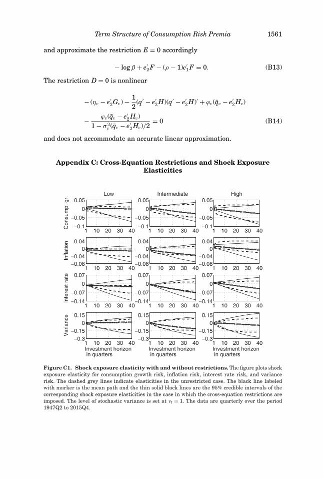
Term Structure of Consumption Risk Premia 1561
and approximate the restriction E = 0 accordingly
− log β + e′2 F − (ρ − 1)e′
1 F = 0. (B13)
The restriction D = 0 is nonlinear
− (ηv − e′2Gv) − 1
2(q′ − e′
2 H)(q′ − e′2 H)′ + ϕv(qv − e′
2 Hv)
− ϕv(qv − e′2 Hv)
1 − σ 2v (qv − e′
2 Hv)/2= 0 (B14)
and does not accommodate an accurate linear approximation.
Appendix C: Cross-Equation Restrictions and Shock ExposureElasticities
1 10 20 30 40−0.1
−0.05
0
0.05
Con
sum
p. g
r.
Low
1 10 20 30 40−0.1
−0.05
0
0.05Intermediate
1 10 20 30 40−0.1
−0.05
0
0.05High
1 10 20 30 40−0.08−0.04
00.04
Infla
tion
1 10 20 30 40−0.08−0.04
00.04
1 10 20 30 40−0.08−0.04
00.04
1 10 20 30 40−0.14
−0.07
0
0.07
Inte
rest
rat
e
1 10 20 30 40−0.14
−0.07
0
0.07
1 10 20 30 40−0.14
−0.07
0
0.07
1 10 20 30 40−0.3
−0.150
0.15
Var
ianc
e
Investment horizon in quarters
1 10 20 30 40−0.3
−0.150
0.15
Investment horizon in quarters
1 10 20 30 40−0.3
−0.150
0.15
Investment horizon in quarters
Figure C1. Shock exposure elasticity with and without restrictions. The figure plots shockexposure elasticity for consumption growth risk, inflation risk, interest rate risk, and variancerisk. The dashed grey lines indicate elasticities in the unrestricted case. The black line labeledwith marker is the mean path and the thin solid black lines are the 95% credible intervals of thecorresponding shock exposure elasticities in the case in which the cross-equation restrictions areimposed. The level of stochastic variance is set at vt = 1. The data are quarterly over the period1947Q2 to 2015Q4.
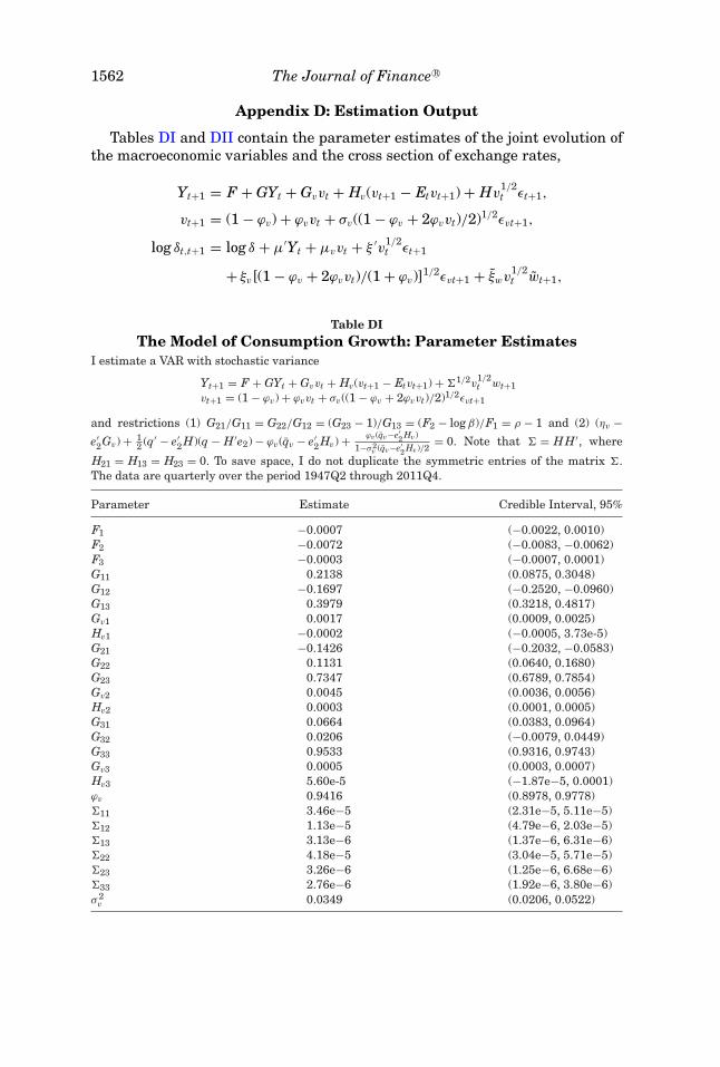
1562 The Journal of Finance R©
Appendix D: Estimation Output
Tables DI and DII contain the parameter estimates of the joint evolution ofthe macroeconomic variables and the cross section of exchange rates,
Yt+1 = F + GYt + Gvvt + Hv(vt+1 − Etvt+1) + Hv1/2t εt+1,
vt+1 = (1 − ϕv) + ϕvvt + σv((1 − ϕv + 2ϕvvt)/2)1/2εvt+1,
log δt,t+1 = log δ + μ′Yt + μvvt + ξ ′v1/2t εt+1
+ ξv[(1 − ϕv + 2ϕvvt)/(1 + ϕv)]1/2εvt+1 + ξwv1/2t wt+1,
Table DIThe Model of Consumption Growth: Parameter Estimates
I estimate a VAR with stochastic variance
Yt+1 = F + GYt + Gvvt + Hv(vt+1 − Etvt+1) + 1/2v1/2t wt+1
vt+1 = (1 − ϕv) + ϕvvt + σv((1 − ϕv + 2ϕvvt)/2)1/2εvt+1
and restrictions (1) G21/G11 = G22/G12 = (G23 − 1)/G13 = (F2 − log β)/F1 = ρ − 1 and (2) (ηv −e′
2Gv) + 12 (q′ − e′
2 H)(q − H′e2) − ϕv(qv − e′2 Hv) + ϕv (qv−e′
2 Hv )1−σ2
v (qv−e′2 Hv )/2
= 0. Note that = HH′, where
H21 = H13 = H23 = 0. To save space, I do not duplicate the symmetric entries of the matrix .The data are quarterly over the period 1947Q2 through 2011Q4.
Parameter Estimate Credible Interval, 95%
F1 −0.0007 (−0.0022, 0.0010)F2 −0.0072 (−0.0083, −0.0062)F3 −0.0003 (−0.0007, 0.0001)G11 0.2138 (0.0875, 0.3048)G12 −0.1697 (−0.2520, −0.0960)G13 0.3979 (0.3218, 0.4817)Gv1 0.0017 (0.0009, 0.0025)Hv1 −0.0002 (−0.0005, 3.73e-5)G21 −0.1426 (−0.2032, −0.0583)G22 0.1131 (0.0640, 0.1680)G23 0.7347 (0.6789, 0.7854)Gv2 0.0045 (0.0036, 0.0056)Hv2 0.0003 (0.0001, 0.0005)G31 0.0664 (0.0383, 0.0964)G32 0.0206 (−0.0079, 0.0449)G33 0.9533 (0.9316, 0.9743)Gv3 0.0005 (0.0003, 0.0007)Hv3 5.60e-5 (−1.87e−5, 0.0001)ϕv 0.9416 (0.8978, 0.9778)11 3.46e−5 (2.31e−5, 5.11e−5)12 1.13e−5 (4.79e−6, 2.03e−5)13 3.13e−6 (1.37e−6, 6.31e−6)22 4.18e−5 (3.04e−5, 5.71e−5)23 3.26e−6 (1.25e−6, 6.68e−6)33 2.76e−6 (1.92e−6, 3.80e−6)σ 2
v 0.0349 (0.0206, 0.0522)

Term Structure of Consumption Risk Premia 1563
Table DIIExchange Rate Growth Process: Parameter Estimates
I estimate jointly the exchange rate growth process
log δt,t+1 = log δ + μ′Yt + μvvt + ξ ′v1/2t εt+1
+ ξv[(1 − ϕv + 2ϕvvt)/(1 + ϕv)]1/2εvt+1 + ξwv1/2t wt+1
for the three currency baskets, where vectors μ = (μg, μπ , μi)′ and ξ = (ξg, ξπ , ξi)′. Parenthesescontain the 95% credible intervals. The data are quarterly over the period 1986Q2 to 2011Q4.
“Low” “Intermediate” “High” “HML”
log δ −0.0054 0.0308 0.0037 0.0091(−0.1000, 0.0758) (−0.0876, 0.1357) (−0.1625, 0.1718) (−0.1947, 0.1906)
μg 0.9421 −0.7309 −2.1961 −3.1382(0.3288, 1.6178) (−1.3336, −0.1089) (−3.1215, −1.4105) (−4.3207, −2.0893)
μπ −0.5363 −2.0506 −0.9552 −0.4189(−1.0231, 0.0003) (−2.5669, −1.5065) (−1.6249, −0.3365) (−1.2812, 0.4175)
μi −0.2292 2.0813 1.2081 1.4374(−1.0137, 0.6110) (1.3435, 2.9214) (0.4373, 2.0483) (0.3099, 2.5729)
μv −0.0144 0.0076 0.0099 0.0242,(−0.0949, 0.0522) (−0.0427, 0.0356) (−0.0056, 0.0251) (−0.0389, 0.1065)
ξg 0.0017 0.0091 0.0102 0.0085(−0.0251, 0.0398) (−0.0079, 0.0355) (0.0059, 0.0146) (−0.0286, 0.0369)
ξπ −0.0005 0.0150 0.0286 0.0291(−0.0215, 0.0141) (−0.0012, 0.0274) (0.0228, 0.0347) (0.0132, 0.0508)
ξi −0.0148 −0.0121 0.0070 0.0218(−0.0326, −0.0016) (−0.0250, −0.0029) (0.0043, 0.0095) (0.0089, 0.0402)
ξv −0.0015 0.0001 −0.0002 0.0013(−0.0170, 0.0151) (−0.0114, 0.0156) (−0.0115, 0.0106) (−0.0185, 0.0211)
47:II 59:III 72:I 84:III 97:I 09:III0
1
2
3
4
Sto
chas
tic v
aria
nce
Figure D1. Stochastic variance factor. The figure plots a common stochastic variance factorof consumption growth, inflation, nominal interest rate, and exchange rate growth. The thick lineis the estimated mean path. The thin lines corresponds to the 95% credible interval. The data arequarterly from 1947Q2 to 2011Q4. Grey bars indicate the NBER recessions.
with cross-equation restrictions derived under recursive preferences,
G21
G11= G22
G12= G23 − 1
G13= ρ − 1,

1564 The Journal of Finance R©
− log β + e′2 F − (ρ − 1)e′
1 F = 0,
− (ηv − e′2Gv) − 1
2(q′ − e′
2 H)(q′ − e′2 H)′ + ϕv(qv − e′
2 Hv)
− ϕv(qv − e′2 Hv)
1 − σ 2v (qv − e′
2 Hv)/2= 0.
Figure D1 displays the estimated dynamics of the stochastic variance factorvt. The Internet Appendix (Section VII) describes properties of the estimatedmacro dynamics.
REFERENCES
Backus, David K., Nina Boyarchenko, and Mikhail Chernov, 2016, Term structure of asset pricesand returns, Working paper, NYU Stern.
Backus, David K., Mikhail Chernov, and Stanley E. Zin, 2014, Sources of entropy in representativeagent models, Journal of Finance 69, 51–99.
Backus, David K., Silverio Foresi, and Christopher I. Telmer, 2001, Affine term structure modelsand the forward premium anomaly, Journal of Finance 56, 279–304.
Backus, David K., Federico Gavazzoni, Christopher Telmer, and Stanley E. Zin, 2010, Monetarypolicy and the uncovered interest rate parity puzzle, NBER Working paper 16218.
Bansal, Ravi, Dana Kiku, Ivan Shaliastovich, and Amir Yaron, 2014, Volatility, the macroeconomyand asset prices, Journal of Finance 69, 2471–2511.
Bansal, Ravi, Dana Kiku, and Amir Yaron, 2012, Risks for the long run: Estimation with timeaggregation, Working paper, Duke University.
Bansal, Ravi, and Ivan Shaliastovich, 2013, A long-run risks explanation of predictability puzzlesin bond and currency markets, Review of Financial Studies 26, 1–33.
Bansal, Ravi, and Amir Yaron, 2004, Risks for the long run: A potential resolution of asset pricingpuzzles, Journal of Finance 59, 1481–1509.
Borovicka, Jaroslav, and Lars P. Hansen, 2014, Examining macroeconomic models through thelens of asset pricing, Journal of Econometrics 183, 67–90.
Borovicka, Jaroslav, Lars P. Hansen, Mark Hendricks, and Jose A. Scheinkman, 2011, Risk-pricedynamics, Journal of Financial Econometrics 9, 3–65.
Burnside, Craig, Martin Eichenbaum, Isaac Kleshchelski, and Sergio Rebelo, 2011, Do peso prob-lems explain the returns to the carry trade? Review of Financial Studies 24, 853–891.
Campbell, John Y., Stefano Giglio, Christopher Polk, and Robert Turley, 2015, An intertemporalCAPM with stochastic volatility, forthcoming, Journal of Financial Economics.
Carriero, Andrea, Todd E. Clark, and Massimiliano Marcellino, 2016, Common drifting volatilityin large Bayesian VARs, Journal of Business and Economic Statistics 34, 375–390.
Colacito, Riccardo, 2009, Six anomalies looking for a model. A consumption-based explanation ofinternational finance puzzles, Working paper, University of North Carolina.
Colacito, Riccardo, and Mariano M. Croce, 2011, Risks for the long run and the real exchange rate,Journal of Political Economy 119, 153–183.
Colacito, Riccardo, and Mariano M. Croce, 2013, International asset pricing with recursive prefer-ences, Journal of Finance 68, 2651–2686.
Colacito, Riccardo, Mariano M. Croce, Federico Gavazzoni, and Robert Ready, 2015, Currency riskfactors in a recursive multi-country economy, Working paper, University of North Carolina.
Constantinides, George M., and Darrell Duffie, 1996, Asset pricing with heterogeneous consumers,Journal of Political Economy 104, 219–240.
Constantinides, George M., and Anisha Ghosh, 2011, Asset pricing tests with long-run risks inconsumption growth, Review of Asset Pricing Studies 1, 96–136.
Cumby, Robert E., 1988, Is it risk? Explaining deviations from uncovered interest parity, Journalof Monetary Economics 22, 279–299.

Term Structure of Consumption Risk Premia 1565
Eichenbaum, Martin, and Charles L. Evans, 1995, Some empirical evidence on the effects of shocksto monetary policy on exchange rates, Quarterly Journal of Economics 110, 975–1009.
Epstein, Larry G., and Stanley E. Zin, 1989, Substitution, risk aversion, and the temporal behaviorof consumption and asset returns: A theoretical framework, Econometrica 57, 937–969.
Fama, Eugene F., 1984, Forward and spot exchange rates, Journal of Monetary Economics 14,319–338.
Farhi, Emmanuel, and Xavier Gabaix, 2016, Rare disasters and exchange rates, Quarterly Journalof Economics 131, 1–52.
Faust, Jon, and John H. Rogers, 2003, Monetary policy’s role in exchange rate behavior, Journalof Monetary Economics 50, 1403–1424.
Gourieroux, Christian, and Joann Jasiak, 2006, Autoregressive gamma processes, Journal of Fore-casting 25, 129–152.
Hall, Robert E., 1978, Stochastic implications of the life cycle-permanent income hypothesis theoryand evidence, Journal of Political Economy 86, 971–987.
Hansen, Lars P., 2012, Dynamic valuation decomposition within stochastic economies, Economet-rica 80, 911–967.
Hansen, Lars P., John C. Heaton, and Nan Li, 2008, Consumption strikes back? Measuring long-runrisk, Journal of Political Economy 116, 260–302.
Hansen, Lars P., and Jose A. Scheinkman, 2009, Long-term risk: An operator approach, Economet-rica 77, 177–234.
Hansen, Lars P., and Jose A. Scheinkman, 2012, Recursive utility in a Markov environment withstochastic growth, Proceedings of the National Academy of Sciences 109, 11967–11972.
Hansen, Lars P., and Kenneth J. Singleton, 1983, Stochastic consumption, risk aversion, and thetemporal behavior of asset returns, Journal of Political Economy 91, 249–265.
Heyerdahl-Larsen, Christian, 2014, Asset prices and real exchange rates with deep habits, Reviewof Financial Studies 27, 3280–3317.
Kandel, Shmuel, and Robert F. Stambaugh, 1990, Expectations and volatility of consumption andasset returns, Review of Financial Studies 3, 207–232.
Kreps, David M., and Evan L. Porteus, 1978, Temporal distribution of uncertainty and dynamicchoice, Econometrica 46, 185–200.
Le, Anh, Kenneth J. Singleton, and Qiang Dai, 2010, Discrete-time dynamic term structure modelswith generalized market prices of risk, Review of Financial Studies 23, 2184–2227.
Lustig, Hanno, Nikolai Roussanov, and Adrien Verdelhan, 2011, Common risk factors in currencymarkets, Review of Financial Studies 24, 3731–3777.
Lustig, Hanno, Andreas Stathopoulos, and Adrian Verdelhan, 2016, Nominal exchange rate sta-tionarity and long-term bond returns, Working paper, Stanford University.
Lustig, Hanno, and Adrien Verdelhan, 2007, The cross section of foreign currency risk premia andconsumption growth risk, American Economic Review 97, 89–117.
Maggiori, Matteo, 2013, Financial intermediation, international risk sharing, and reserve curren-cies, Working paper, Harvard University.
Menkhoff, Lukas, Lucio Sarno, Maik Schmeling, and Andreas Schrimpf, 2012, Carry trades andglobal foreign exchange volatility, Journal of Finance 67, 681–718.
Piazzesi, Monika, and Martin Schneider, 2006, Equilibrium yield curves, in Daron Acemoglu,Kenneth Rogoff, and Michael Woodford, eds.: NBER Macroeconomics Annual (MIT Press,Cambridge, MA).
Rafferty, Barry, 2011, Currency returns, skewness and crash risk, Working paper, University ofMelbourne.
Rubio-Ramirez, Juan F., Daniel F. Waggoner, and Tao Zha, 2010, Structural vector autoregressions:Theory of identification and algorithms for inference, Review of Economic Studies 77, 665–696.
Sarkissian, Sergei, 2003, Incomplete consumption risk sharing and currency risk premiums, Re-view of Financial Studies 16, 983–1005.
Verdelhan, Adrien, 2010, A habit-based explanation of the exchange rate risk premium, Journalof Finance 65, 123–146.
Verdelhan, Adrien, The share of systematic variation in bilateral exchange rates, Journal of Fi-nance (forthcoming).

1566 The Journal of Finance R©
Weil, Philippe, 1990, Nonexpected utility in macroeconomics, Quarterly Journal of Economics 105,29–42.
Whitelaw, Robert F., 2000, Stock market risk and return: An equilibrium approach, Review ofFinancial Studies 13, 521–547.
Wright, Jonathan N., 2011, Term premia and inflation uncertainty: Empirical evidence from aninternational panel dataset, American Economic Review 101, 1514–1534.
Yogo, Motohiro, 2006, A consumption-based explanation of expected stock returns, Journal ofFinance 61, 539–580.
Zviadadze, Irina, 2016, Term structure of risk in macrofinance models, Working paper, StockholmSchool of Economics.
Supporting Information
Additional Supporting Information may be found in the online version of thisarticle at the publisher’s website:
Appendix S1: Internet Appendix.