SANDIA REPORTSAND2007-6702Unlimited ReleasePrinted November 2007

Tensor Decompositions andApplications

Tamara G. Kolda and Brett W. Bader

Prepared bySandia National LaboratoriesAlbuquerque, New Mexico 87185 and Livermore, California 94550

Sandia is a multiprogram laboratory operated by Sandia Corporation,a Lockheed Martin Company, for the United States Department of Energy’sNational Nuclear Security Administration under Contract DE-AC04-94-AL85000.

Approved for public release; further dissemination unlimited.

Issued by Sandia National Laboratories, operated for the United States Department of Energy by SandiaCorporation.

NOTICE: This report was prepared as an account of work sponsored by an agency of the United StatesGovernment. Neither the United States Government, nor any agency thereof, nor any of their employees,nor any of their contractors, subcontractors, or their employees, make any warranty, express or implied,or assume any legal liability or responsibility for the accuracy, completeness, or usefulness of any infor-mation, apparatus, product, or process disclosed, or represent that its use would not infringe privatelyowned rights. Reference herein to any specific commercial product, process, or service by trade name,trademark, manufacturer, or otherwise, does not necessarily constitute or imply its endorsement, recom-mendation, or favoring by the United States Government, any agency thereof, or any of their contractorsor subcontractors. The views and opinions expressed herein do not necessarily state or reflect those ofthe United States Government, any agency thereof, or any of their contractors.

Printed in the United States of America. This report has been reproduced directly from the best availablecopy.

Available to DOE and DOE contractors fromU.S. Department of EnergyOffice of Scientific and Technical InformationP.O. Box 62Oak Ridge, TN 37831

Telephone: (865) 576-8401Facsimile: (865) 576-5728E-Mail: reports@adonis.osti.govOnline ordering: http://www.osti.gov/bridge

Available to the public fromU.S. Department of CommerceNational Technical Information Service5285 Port Royal RdSpringfield, VA 22161

Telephone: (800) 553-6847Facsimile: (703) 605-6900E-Mail: orders@ntis.fedworld.govOnline ordering: http://www.ntis.gov/help/ordermethods.asp?loc=7-4-0#online

DE

PA

RT

MENT OF EN

ER

GY

• • UN

IT

ED

STATES OFA

M

ER

IC

A

2

SAND2007-6702Unlimited Release

Printed November 2007

Tensor Decompositions and Applications

Tamara G. KoldaMathematics, Informatics, and Decisions Sciences Department

Sandia National LaboratoriesLivermore, CA 94551-9159

tgkolda@sandia.gov

Brett W. BaderComputer Science and Informatics Department

Sandia National LaboratoriesAlbuquerque, NM 87185-1318

bwbader@sandia.gov

Abstract

This survey provides an overview of higher-order tensor decompositions,their applications, and available software. A tensor is a multidimensional orN -way array. Decompositions of higher-order tensors (i.e., N -way arrays withN ≥ 3) have applications in psychometrics, chemometrics, signal processing,numerical linear algebra, computer vision, numerical analysis, data mining,neuroscience, graph analysis, etc. Two particular tensor decompositions can beconsidered to be higher-order extensions of the matrix singular value decompo-sition: CANDECOMP/PARAFAC (CP) decomposes a tensor as a sum of rank-one tensors, and the Tucker decomposition is a higher-order form of principalcomponents analysis. There are many other tensor decompositions, includ-ing INDSCAL, PARAFAC2, CANDELINC, DEDICOM, and PARATUCK2 aswell as nonnegative variants of all of the above. The N-way Toolbox and Ten-sor Toolbox, both for MATLAB, and the Multilinear Engine are examples ofsoftware packages for working with tensors.

3

Acknowledgments

The following workshops have greatly influenced our understanding and appreciationof tensor decompositions: Workshop on Tensor Decompositions, American Instituteof Mathematics, Palo Alto, California, USA, July 19–23, 2004; Workshop on TensorDecompositions and Applications (WTDA), CIRM, Luminy, Marseille, France, Au-gust 29–September 2, 2005; and Three-way Methods in Chemistry and Psychology,Chania, Crete, Greece, June 4–9, 2006. Consequently, we thank the organizers andthe supporting funding agencies.

The following people were kind enough to read earlier versions of this manuscriptand offer helpful advice on many fronts: Evrim Acar-Ataman, Rasmus Bro, PeterChew, Lieven De Lathauwer, Lars Elden, Philip Kegelmeyer, Morten Mørup, TeresaSelee, and Alwin Stegeman. We also wish to acknowledge the following for theirhelpful conversations and pointers to related literature: Dario Bini, Pierre Comon,Gene Golub, Richard Harshman, Henk Kiers, Pieter Kroonenberg, Lek-Heng Lim,Berkant Savas, Nikos Sidiropoulos, Jos Ten Berge, and Alex Vasilescu.

4

Contents

1 Introduction . . . . . . . . . . . . . . . . . . . . . . . . . . . . . . . . . . . . . . . . . . . . . . . . . . . . . . . . . . . . . . 92 Notation and preliminaries . . . . . . . . . . . . . . . . . . . . . . . . . . . . . . . . . . . . . . . . . . . . . . . . 11

2.1 Rank-one tensors . . . . . . . . . . . . . . . . . . . . . . . . . . . . . . . . . . . . . . . . . . . . 122.2 Symmetry and tensors . . . . . . . . . . . . . . . . . . . . . . . . . . . . . . . . . . . . . . . . 132.3 Diagonal tensors . . . . . . . . . . . . . . . . . . . . . . . . . . . . . . . . . . . . . . . . . . . . . 132.4 Matricization: transforming a tensor into a matrix . . . . . . . . . . . . . . . . . 142.5 Tensor multiplication: the n-mode product . . . . . . . . . . . . . . . . . . . . . . . 142.6 Matrix Kronecker, Khatri-Rao, and Hadamard products . . . . . . . . . . . . 16

3 Tensor rank and the CANDECOMP/PARAFAC decomposition. . . . . . . . . . . . 193.1 Tensor rank . . . . . . . . . . . . . . . . . . . . . . . . . . . . . . . . . . . . . . . . . . . . . . . . . 203.2 Uniqueness . . . . . . . . . . . . . . . . . . . . . . . . . . . . . . . . . . . . . . . . . . . . . . . . . 233.3 Low-rank approximations and the border rank . . . . . . . . . . . . . . . . . . . . 253.4 Computing the CP decomposition . . . . . . . . . . . . . . . . . . . . . . . . . . . . . . . 283.5 Applications of CP . . . . . . . . . . . . . . . . . . . . . . . . . . . . . . . . . . . . . . . . . . . 30

4 Compression and the Tucker decomposition. . . . . . . . . . . . . . . . . . . . . . . . . . . . . . . . 334.1 The n-rank . . . . . . . . . . . . . . . . . . . . . . . . . . . . . . . . . . . . . . . . . . . . . . . . . 354.2 Computing the Tucker decomposition . . . . . . . . . . . . . . . . . . . . . . . . . . . . 364.3 Lack of uniqueness and methods to overcome it . . . . . . . . . . . . . . . . . . . . 384.4 Applications of Tucker . . . . . . . . . . . . . . . . . . . . . . . . . . . . . . . . . . . . . . . . 38

5 Other decompositions . . . . . . . . . . . . . . . . . . . . . . . . . . . . . . . . . . . . . . . . . . . . . . . . . . . . . 415.1 INDSCAL . . . . . . . . . . . . . . . . . . . . . . . . . . . . . . . . . . . . . . . . . . . . . . . . . . 415.2 PARAFAC2 . . . . . . . . . . . . . . . . . . . . . . . . . . . . . . . . . . . . . . . . . . . . . . . . 425.3 CANDELINC . . . . . . . . . . . . . . . . . . . . . . . . . . . . . . . . . . . . . . . . . . . . . . . 445.4 DEDICOM . . . . . . . . . . . . . . . . . . . . . . . . . . . . . . . . . . . . . . . . . . . . . . . . . 455.5 PARATUCK2 . . . . . . . . . . . . . . . . . . . . . . . . . . . . . . . . . . . . . . . . . . . . . . . 485.6 Nonnegative tensor factorizations . . . . . . . . . . . . . . . . . . . . . . . . . . . . . . . 495.7 More decompositions . . . . . . . . . . . . . . . . . . . . . . . . . . . . . . . . . . . . . . . . . 51

6 Software for tensors . . . . . . . . . . . . . . . . . . . . . . . . . . . . . . . . . . . . . . . . . . . . . . . . . . . . . . . 537 Discussion. . . . . . . . . . . . . . . . . . . . . . . . . . . . . . . . . . . . . . . . . . . . . . . . . . . . . . . . . . . . . . . . . 55References . . . . . . . . . . . . . . . . . . . . . . . . . . . . . . . . . . . . . . . . . . . . . . . . . . . . . . . . . . . . . . . . . . . . 56

5

Figures

1 A third-order tensor . . . . . . . . . . . . . . . . . . . . . . . . . . . . . . . . . . . . . . . . . . 92 Fibers of a 3rd-order tensor. . . . . . . . . . . . . . . . . . . . . . . . . . . . . . . . . . . . 113 Slices of a 3rd-order tensor. . . . . . . . . . . . . . . . . . . . . . . . . . . . . . . . . . . . . 124 Rank-one third-order tensor . . . . . . . . . . . . . . . . . . . . . . . . . . . . . . . . . . . 135 Three-way identity tensor . . . . . . . . . . . . . . . . . . . . . . . . . . . . . . . . . . . . . 136 CP decomposition of a three-way array. . . . . . . . . . . . . . . . . . . . . . . . . . . 207 Illustration of a sequence of tensors converging to one of higher rank . . 278 Alternating least squares algorithm to compute a CP decomposition . . . 299 Tucker decomposition of a three-way array . . . . . . . . . . . . . . . . . . . . . . . 3410 Truncated Tucker decomposition of a three-way array . . . . . . . . . . . . . . 3511 Tucker’s “Method I” or the HO-SVD . . . . . . . . . . . . . . . . . . . . . . . . . . . . 3612 Alternating least squares algorithm to compute a Tucker decomposition 3713 Illustration of PARAFAC2. . . . . . . . . . . . . . . . . . . . . . . . . . . . . . . . . . . . . 4314 Three-way DEDICOM model. . . . . . . . . . . . . . . . . . . . . . . . . . . . . . . . . . . 4715 General PARATUCK2 model. . . . . . . . . . . . . . . . . . . . . . . . . . . . . . . . . . . 4816 Block decomposition of a third-order tensor. . . . . . . . . . . . . . . . . . . . . . . 51

6

Tables

1 Some of the many names for the CP decomposition. . . . . . . . . . . . . . . . . 192 Maximum ranks over R for three-way tensors. . . . . . . . . . . . . . . . . . . . . . 213 Typical rank over R for three-way tensors. . . . . . . . . . . . . . . . . . . . . . . . . 224 Typical rank over R for three-way tensors with symmetric frontal slices 235 Comparison of typical ranks over R for three-way tensors with and

without symmetric frontal slices . . . . . . . . . . . . . . . . . . . . . . . . . . . . . . . . 236 Names for the Tucker decomposition . . . . . . . . . . . . . . . . . . . . . . . . . . . . 337 Other tensor decompositions. . . . . . . . . . . . . . . . . . . . . . . . . . . . . . . . . . . 41

7

This page intentionally left blank.

8

1 Introduction

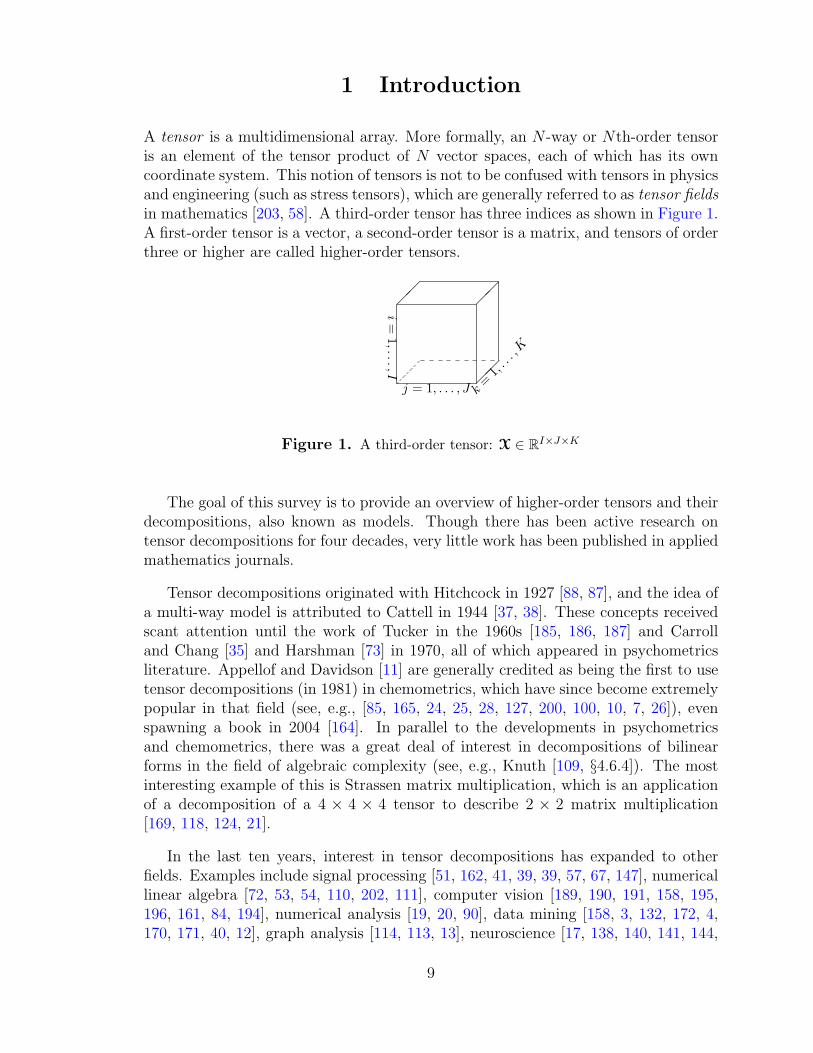
A tensor is a multidimensional array. More formally, an N -way or Nth-order tensoris an element of the tensor product of N vector spaces, each of which has its owncoordinate system. This notion of tensors is not to be confused with tensors in physicsand engineering (such as stress tensors), which are generally referred to as tensor fieldsin mathematics [203, 58]. A third-order tensor has three indices as shown in Figure 1.A first-order tensor is a vector, a second-order tensor is a matrix, and tensors of orderthree or higher are called higher-order tensors.

��

��

��

i=

1,...,I

j = 1, . . . , J k=

1,. .. ,K

Figure 1. A third-order tensor: X ∈ RI×J×K

The goal of this survey is to provide an overview of higher-order tensors and theirdecompositions, also known as models. Though there has been active research ontensor decompositions for four decades, very little work has been published in appliedmathematics journals.

Tensor decompositions originated with Hitchcock in 1927 [88, 87], and the idea ofa multi-way model is attributed to Cattell in 1944 [37, 38]. These concepts receivedscant attention until the work of Tucker in the 1960s [185, 186, 187] and Carrolland Chang [35] and Harshman [73] in 1970, all of which appeared in psychometricsliterature. Appellof and Davidson [11] are generally credited as being the first to usetensor decompositions (in 1981) in chemometrics, which have since become extremelypopular in that field (see, e.g., [85, 165, 24, 25, 28, 127, 200, 100, 10, 7, 26]), evenspawning a book in 2004 [164]. In parallel to the developments in psychometricsand chemometrics, there was a great deal of interest in decompositions of bilinearforms in the field of algebraic complexity (see, e.g., Knuth [109, §4.6.4]). The mostinteresting example of this is Strassen matrix multiplication, which is an applicationof a decomposition of a 4 × 4 × 4 tensor to describe 2 × 2 matrix multiplication[169, 118, 124, 21].

In the last ten years, interest in tensor decompositions has expanded to otherfields. Examples include signal processing [51, 162, 41, 39, 39, 57, 67, 147], numericallinear algebra [72, 53, 54, 110, 202, 111], computer vision [189, 190, 191, 158, 195,196, 161, 84, 194], numerical analysis [19, 20, 90], data mining [158, 3, 132, 172, 4,170, 171, 40, 12], graph analysis [114, 113, 13], neuroscience [17, 138, 140, 141, 144,

9

142, 143, 1, 2] and more. Several surveys have already been written in other fields;see [116, 45, 86, 24, 25, 41, 108, 66, 42, 164, 58, 26, 5]. Moreover, there are severalsoftware packages for working with tensors [149, 9, 123, 70, 14, 15, 16, 198, 201].

Wherever possible, the references in this review include a hyperlink to either thepublisher web page for the paper or the author’s version. Many older papers are nowavailable online in PDF format. We also direct the reader to P. Kroonenberg’s three-mode bibliography1, which includes several out-of-print books and theses (includinghis own [116]). Likewise, R. Harshman’s web site2 has many hard-to-find papers,including his original 1970 PARAFAC paper [73] and Kruskal’s 1989 paper [120]which is now out of print.

The sequel is organized as follows. Section 2 describes the notation and commonoperations used throughout the review; additionally, we provide pointers to otherpapers that discuss notation. Both the CANDECOMP/PARAFAC (CP) [35, 73] andTucker [187] tensor decompositions can be considered higher-order generalization ofthe matrix singular value decomposition (SVD) and principal component analysis(PCA). In §3, we discuss the CP decomposition, its connection to tensor rank andtensor border rank, conditions for uniqueness, algorithms and computational issues,and applications. The Tucker decomposition is covered in §4, where we discuss its re-lationship to compression, the notion of n-rank, algorithms and computational issues,and applications. Section 5 covers other decompositions, including INDSCAL [35],PARAFAC2 [75], CANDELINC [36], DEDICOM [76], and PARATUCK2 [83], andtheir applications. §6 provides information about software for tensor computations.We summarize our findings in §7.

1http://three-mode.leidenuniv.nl/bibliogr/bibliogr.htm2http://publish.uwo.ca/~harshman/

10

2 Notation and preliminaries

In this review, we have tried to remain as consistent as possible with terminologythat would be familiar to applied mathematicians and the terminology of previouspublications in the area of tensor decompositions. The notation used here is verysimilar to that proposed by Kiers [101]. Other standards have been proposed as well;see Harshman [77] and Harshman and Hong [79].

Tensors (i.e., multi-way arrays) are denoted by boldface Euler script letters, e.g.,X. The order of a tensor is the number of dimensions, also known as ways or modes.3

Matrices are denoted by boldface capital letters, e.g., A; vectors are denoted byboldface lowercase letters, e.g., a; and scalars are denoted by lowercase letters, e.g.,a. The ith entry of a vector a is denoted by ai, element (i, j) of a matrix A by aij,and element (i, j, k) element of a third-order tensor X by xijk. Indices typically rangefrom 1 to their capital version, e.g., i = 1, . . . , I. The nth element in a sequenceis denoted by a superscript in parentheses, e.g., A(n) denotes the nth matrix in asequence.

Subarrays are formed when a subset of the indices is fixed. For matrices, theseare the rows and columns. A colon is used to indicate all elements of a mode. Thus,the jth column of A is denoted by a:j; likewise, the ith row of a matrix A is denotedby ai:.

Fibers are the higher order analogue of matrix rows and columns. A fiber isdefined by fixing every index but one. A matrix column is a mode-1 fiber and amatrix row is a mode-2 fiber. Third-order tensors have column, row, and tube fibers,denoted by x:jk, xi:k, and xij:, respectively; see Figure 2. Fibers are always assumedto be column vectors.

(a) Mode-1 (column) fibers:x:jk

(b) Mode-2 (row) fibers:xi:k

��

��

��

��

��

��

��

��

��

��

��

��

��

��

��

��

��

��

��

��

��

��

��

��

��

��

��

��

��

��

��

��

��

��

��

��

��

��

��

��

��

��

��

��

��

��

��

��

��

��

��

��

��

��

(c) Mode-3 (tube) fibers:xij:

Figure 2. Fibers of a 3rd-order tensor.

3In some fields, the order of the tensor is referred to as the rank of the tensor. In much of theliterature and this review, however, the term rank means something quite different; see §3.1.

11

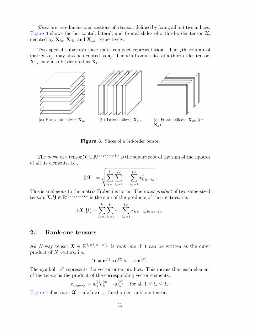
Slices are two-dimensional sections of a tensor, defined by fixing all but two indices.Figure 3 shows the horizontal, lateral, and frontal slides of a third-order tensor X,denoted by Xi::, X:j:, and X::k, respectively.

Two special subarrays have more compact representation. The jth column ofmatrix, a:j, may also be denoted as aj. The kth frontal slice of a third-order tensor,X::k may also be denoted as Xk.

��

��

��

��

��

��

��

��

��

��

��

��

��

��

��

��

��

��

��

��

��

��

��

��

��

��

��

��

��

��

(a) Horizontal slices: Xi::

��

��

��

��

��

��

��

��

��

��

��

��

��

��

��

��

��

��

��

��

��

��

��

��

��

��

��

��

��

��

(b) Lateral slices: X:j: (c) Frontal slices: X::k (orXk)

Figure 3. Slices of a 3rd-order tensor.

The norm of a tensor X ∈ RI1×I2×···×IN is the square root of the sum of the squaresof all its elements, i.e.,

‖X ‖ =

√√√√ I1∑i1=1

I2∑i2=1

· · ·IN∑

iN=1

x2i1i2···iN .

This is analogous to the matrix Frobenius norm. The inner product of two same-sizedtensors X, Y ∈ RI1×I2×···×IN is the sum of the products of their entries, i.e.,

〈X, Y 〉 =

I1∑i1=1

I2∑i2=1

· · ·IN∑

iN=1

xi1i2···iN yi1i2···iN .

2.1 Rank-one tensors

An N -way tensor X ∈ RI1×I2×···×IN is rank one if it can be written as the outerproduct of N vectors, i.e.,

X = a(1) ◦ a(2) ◦ · · · ◦ a(N).

The symbol “◦” represents the vector outer product. This means that each elementof the tensor is the product of the corresponding vector elements:

xi1i2···iN = a(1)i1

a(2)i2· · · a(N)

iNfor all 1 ≤ in ≤ In.

Figure 4 illustrates X = a ◦ b ◦ c, a third-order rank-one tensor.

12

���

���

���

X

=�

���

��

���

a

b

c

Figure 4. Rank-one third-order tensor, X = a ◦ b ◦ c.

2.2 Symmetry and tensors

A tensor is called cubical if every mode is the same size, i.e., X ∈ RI×I×I×···×I [43].A cubical tensor is called supersymmetric (though this term is challenged by Comonet al. [43] who instead prefer just “symmetric”) if its elements remain constant underany permutation of the indices. For instance, a three-way tensor X ∈ RI×I×I issupersymmetric if

xijk = xikj = xjik = xjki = xkij = xkji for all i, j, k = 1, . . . , I.

Tensors can be (partially) symmetric in two or more modes as well. For example,a three-way tensor X ∈ RI×I×K is symmetric in modes one and two if all its frontalslices are symmetric, i.e.,

Xk = XTk for all k = 1, . . . , K.

2.3 Diagonal tensors

A tensor X ∈ RI1×I2×···×IN is diagonal if xi1i2···iN 6= 0 only if i1 = i2 = · · · = iN .We use I to denote the identity tensor with ones on the superdiagonal and zeroselsewhere; see Figure 5.

��

��

��

1 1 1 1 1 1 1 1 1

Figure 5. Three-way identity tensor: I ∈ RI×I×I

13

2.4 Matricization: transforming a tensor into a matrix

Matricization, also known as unfolding or flattening, is the process of reordering theelements of an N -way array into a matrix. For instance, a 2 × 3 × 4 tensor canbe arranged as a 6 × 4 matrix or a 2 × 8 matrix, etc. In this review, we consideronly the special case of mode-n matricization because it is the only form relevant toour discussion. A more general treatment of matricization can be found in Kolda[112]. The mode-n matricization of a tensor X ∈ RI1×I2×···×IN is denoted by X(n) andarranges the mode-n fibers to be the columns of the matrix. Though conceptuallysimple, the formal notation is clunky. Tensor element (i1, i2, . . . , iN) maps to matrixelement (in, j) where

j = 1 +N∑

k=1k 6=n

(ik − 1)Jk, with Jk =k−1∏m=1m6=n

Im.

The concept is easier to understand using an example. Let the frontal slices of X ∈R3×4×2 be

X1 =

1 4 7 102 5 8 113 6 9 12

, X2 =

13 16 19 2214 17 20 2315 18 21 24

. (1)

Then, the three mode-n unfoldings are:

X(1) =

1 4 7 10 13 16 19 222 5 8 11 14 17 20 233 6 9 12 15 18 21 24

,

X(2) =

1 2 3 13 14 154 5 6 16 17 187 8 9 19 20 2110 11 12 22 23 24

,

X(3) =

[1 2 3 4 5 · · · 9 10 11 1213 14 15 16 17 · · · 21 22 23 24

].

2.5 Tensor multiplication: the n-mode product

Tensors can be multiplied together, though obviously the notation and symbols forthis are much more complex than for matrices. For a full treatment of tensor multi-plication see, e.g., Bader and Kolda [14]. Here we consider only the tensor n-modeproduct, i.e., multiplying a tensor by a matrix (or a vector) in mode n.

The n-mode (matrix) product of a tensor X ∈ RI1×I2×···×IN with a matrix U ∈RJ×In is denoted by X ×n U and is of size I1 × · · · × In−1 × J × In+1 × · · · × IN .

14

Elementwise, we have

(X×n U)i1···in−1j in+1···iN =In∑

in=1

xi1i2···iN ujin .

Each mode-n fiber is multiplied by the matrix U. The idea can also be expressed interms of unfolded tensors:

Y = X×n U ⇔ Y(n) = UX(n).

As an example, let X be the tensor defined above in (1) and let U =

[1 3 52 4 6

].

Then, the product Y = X×1 U ∈ R2×4×2 is

Y1 =

[22 49 76 10328 64 100 136

], Y2 =

[130 157 184 211172 208 244 280

].

A few facts regarding n-mode matrix products are in order; see De Lathauwer et al.[53]. For distinct modes in a series of multiplications, the order of the multiplicationis irrelevant, i.e.,

X×m A×n B = X×n B×m A (m 6= n).

If the modes are the same, then

X×n A×n B = X×n (BA).

The n-mode (vector) product of a tensor X ∈ RI1×I2×···×IN with a vector v ∈ RIn

is denoted by X •n v. The result is of order N − 1, i.e., the size is I1 × · · · × In−1 ×In+1 × · · · × IN . Elementwise,

(X •n v)i1···in−1in+1···iN =In∑

in=1

xi1i2···iN vin .

The idea is to compute the inner product of each mode-n fiber with the vector v.

For example, let X be as given in (1) and define v =[1 2 3 4

]T. Then

X •2 v =

70 19080 20090 210

.

When it comes to mode-n vector multiplication, precedence matters because theorder of the intermediate results change. In other words,

X •m a •n b = (X •m a) •n−1 b = (X •n b) •m a for m < n.

15

2.6 Matrix Kronecker, Khatri-Rao, and Hadamard products

Several matrix products are important in the sections that follow, so we briefly definethem here.

The Kronecker product of matrices A ∈ RI×J and B ∈ RK×L is denoted by A⊗B.The result is a matrix of size (IK)× (JL) and defined by

A⊗B =

a11B a12B · · · a1JBa21B a22B · · · a2JB

......

. . ....

aI1B aI2B · · · aIJB

=

[a1 ⊗ b1 a1 ⊗ b2 a1 ⊗ b3 · · · aJ ⊗ bL−1 aJ ⊗ bL

].

The Khatri-Rao product [164] is the “matching columnwise” Kronecker product.Given matrices A ∈ RI×K and B ∈ RJ×K , their Khatri-Rao product is denoted byA�B. The result is a matrix of size (IJ)×K and defined by

A�B =[a1 ⊗ b1 a2 ⊗ b2 · · · aK ⊗ bK

].

If a and b are vectors, then the Khatri-Rao and Kronecker products are identical,i.e., a⊗ b = a� b.

The Hadamard product is the elementwise matrix product. Given matrices A andB, both of size I × J , their Hadamard product is denoted by A ∗ B. The result isalso size I × J and defined by

A ∗B =

a11b11 a12b12 · · · a1Jb1J

a21b21 a22b22 · · · a2Jb2J...

.... . .

...aI1bI1 aI2bI2 · · · aIJbIJ

.

These matrix products have properties [188, 164] that will prove useful in ourdiscussions:

(A⊗B)(C⊗D) = AC⊗BD,

(A⊗B)† = A† ⊗B†,

A�B�C = (A�B)�C = A� (B�C),

(A�B)T(A�B) = ATA ∗BTB,

(A�B)† = ((ATA) ∗ (BTB))†(A�B)T. (2)

As an example of the utility of the Kronecker product, consider the following.Let X ∈ RI1×I2×···×IN and A(n) ∈ RJn×In for all n ∈ {1, . . . , N}. Then, for any

16

n ∈ {1, . . . , N} we have

Y = X×1 A(1) ×2 A(2) · · · ×N A(N) ⇔

Y(n) = A(n)X(n)

(A(N) ⊗ · · · ⊗A(n+1) ⊗A(n−1) ⊗ · · · ⊗A(1)

)T

.

17

This page intentionally left blank.

18

3 Tensor rank and the

CANDECOMP/PARAFAC decomposition

In 1927, Hitchcock [87, 88] proposed the idea of the polyadic form of a tensor, i.e.,expressing a tensor as the sum of a finite number of rank-one tensors; and later, in1944, Cattell [37, 38] proposed ideas for parallel proportional analysis and the idea ofmultiple axes for analysis (circumstances, objects, and features). The concept finallybecame popular after its third introduction, in 1970 to the psychometrics commu-nity, in the form of CANDECOMP (canonical decomposition) by Carroll and Chang[35] and PARAFAC (parallel factors) by Harshman [73]. We refer to the CANDE-COMP/PARAFAC decomposition as CP, per Kiers [101]. Table 1 summarizes thedifferent names for the CP decomposition.

Name Proposed byPolyadic Form of a Tensor Hitchcock [87]PARAFAC (Parallel Factors) Harshman [73]CANDECOMP or CAND (Canonical decomposition) Carroll and Chang [35]CP (CANDECOMP/PARAFAC) Kiers [101]

Table 1. Some of the many names for the CP decomposi-tion.

CP decomposes a tensor into a sum of component rank-one tensors. For example,given a third-order tensor X ∈ RI×J×K , we wish to write it as

X ≈R∑

r=1

ar ◦ br ◦ cr, (3)

where R is a positive integer, and ar ∈ RI , br ∈ RJ , and cr ∈ RK , for r = 1, . . . , R.Elementwise, (3) is written as

xijk ≈R∑

r=1

air bjr ckr, for i = 1, . . . , I, j = 1, . . . , J, k = 1, . . . , K.

This is illustrated in Figure 6.

The factor matrices refer to the combination of the vectors from the rank-onecomponents, i.e., A =

[a1 a2 · · · aR

]and likewise for B and C. Using these, the

three matricized versions (one per mode; see §2.4) of (3) are:

X(1) ≈ A(C�B)T,

X(2) ≈ B(C�A)T,

X(3) ≈ C(B�A)T.

19

X

= ...+ + +

c1 c2

aR

b1

a1

b2

a2

bR

cR

Figure 6. CP decomposition of a three-way array.

Recall that � denotes the Khatri-Rao product from §2.6. The three-way model issometimes written in terms of the frontal slices of X (see Figure 3):

Xk ≈ AD(k)BT where D(k) ≡ diag(ck:) for k = 1, . . . , K.

Analogous equations can be written for the horizontal and lateral slices. In general,though, slice-wise expressions do not easily extend beyond three dimensions. Follow-ing Kolda [112] (see also Kruskal [118]), the CP model can be concisely expressedas

X ≈ JA,B,CK.It is often useful to assume that the columns of A, B, and C are normalized to lengthone with the weights absorbed into the vector λ ∈ RR so that

X ≈R∑

r=1

λr ar ◦ br ◦ cr. = Jλ ;A,B,CK. (4)

We have focused on the three-way case because it is widely applicable and suf-ficient for many needs. For a general Nth-order tensor, X ∈ RI1×I2×···×IN , the CPdecomposition is

X ≈R∑

r=1

λr a(1)r ◦ a(2)

r ◦ · · · ◦ a(N)r = Jλ ;A(1),A(2), . . . ,A(N)K.

where λ ∈ RR and A(n) ∈ RIn×R for n = 1, . . . , N . In this case, the mode-n matricizedversion is given by

X(n) ≈ A(n)Λ(A(N) � · · · �A(n+1) �A(n−1) � · · · �A(1))T,

where Λ = diag(λ).

3.1 Tensor rank

The rank of a tensor X, denoted rank(X), is defined as the smallest number of rank-one tensors (see §2.1) that generate X as their sum [87, 118]. In other words, this

20

is the smallest number of components in an exact CP decomposition. Hitchcock [87]first proposed this definition of rank in 1927, and Kruskal [118] did so independently50 years later. For the perspective of tensor rank from an algebraic complexity point-of-view, see [89, 34, 109, 21] and references therein.

The definition of tensor rank is an exact analogue to the definition of matrix rank,but the properties of matrix and tensor ranks are quite different. For instance, therank of a real-valued tensor may actually be different over R and C. See Kruskal [120]for a complete discussion.

One major difference between matrix and tensor rank is that there is no straight-forward algorithm to determine the rank of a specific given tensor. Kruskal [120] citesan example of a particular 9× 9× 9 tensor whose rank is only known to be boundedbetween 18 and 23 (recent work by Comon et al. [44] conjectures that the rank is 19or 20). In practice, the rank of a tensor is determined numerically by fitting variousrank-R CP models; see §3.4.

Another peculiarity of tensors has to do with maximum and typical ranks. Themaximum rank is defined as the largest attainable rank, whereas the typical rankis any rank that occurs with probability greater than zero when the elements of thetensor are drawn randomly from a uniform continuous distribution. For the collectionof I×J matrices, the maximum and typical ranks are identical and equal to min{I, J}.For tensors, the two ranks may be different and there may be more than one typicalrank. Kruskal [120] discusses the case of 2 × 2 × 2 tensors which have typical ranksof two and three. In fact, Monte Carlo experiments revealed that the set of 2× 2× 2tensors of rank two fills about 79% of the space while those of rank three fill 21%.Rank-one tensors are possible but occur with zero probability. See also the conceptof border rank discussed in §3.3.

For a general third-order tensor X ∈ RI×J×K , only the following weak upperbound on its maximum rank is known [120]:

rank(X) ≤ min{IJ, IK, JK}.

Table 2 shows known maximum ranks for tensors of specific sizes. The most generalresult is for third-order tensors with only two slices.

Tensor Size Maximum Rank CitationI × J × 2 min{I, J}+ min{I, J, bmax{I, J}/2}c} [91, 120]3× 3× 3 5 [120]

Table 2. Maximum ranks over R for three-way tensors.

Table 3 shows some known formulas for the typical ranks of certain three-waytensors. For general I × J × K (or higher order) tensors, recall that the orderingof the modes does not affect the rank, i.e., the rank is constant under permutation.

21

Kruskal [120] discussed the case of 2 × 2 × 2 tensors having typical ranks of bothtwo and three and gives a diagnostic polynomial to determine the rank of a giventensor. Ten Berge [173] later extended this result (and the diagnostic polynomial)to show that I × I × 2 tensors have a typical ranks of I and I + 1. Ten Berge andKiers [177] fully characterize the set of all I × J × 2 arrays and further contrast thedifference between rank over R and C. The typical rank over C of an I×J ×2 tensoris min{I, 2J} when I > J (the same as for R), but the rank is I if I = J (differentthan for R). For general three-way arrays, Ten Berge [174] classifies three-way arraysaccording to the sizes of I, J and K, as follows: A tensor with I > J > K is called“very tall” when I > JK; “tall” when JK − J < I < JK, and “compact” whenI < JK−J . Very tall tensors trivially have maximal and typical rank JK [174]. Talltensors are treated in [174] (and [177] for I×J ×2 arrays). Little is known about thetypical rank of compact tensors except for when I = JK−J [174]. Recent results byComon et al. [44] provide typical ranks for a larger range of tensor sizes.

Tensor Size Typical Rank Citation2× 2× 2 {2, 3} [120]3× 3× 2 {3, 4} [119, 173]5× 3× 3 {5, 6} [175]

I × J × 2 with I ≥ 2J (very tall) 2J [177]I × J × 2 with J < I < 2J (tall) I [177]

I × I × 2 (compact) {I, I + 1} [173, 177]I × J ×K with I ≥ JK (very tall) JK [174]

I × J ×K with JK − J < I < JK (tall) I [174]I × J ×K with I = JK − J (compact) {I, I + 1} [174]

Table 3. Typical rank over R for three-way tensors.

The situation changes somewhat when we restrict the tensors in some way. TenBerge, Sidiropoulos, and Rocci [180] consider the case where the tensor is symmetricin two modes. Without loss of generality, assume that the frontal slices are symmetric;see §2.2. The results are presented in Table 4. It is interesting to compare the resultsfor tensors with and without symmetric slices as is done in Table 5. In some cases,e.g., I × I × 2, the typical rank is the same in either case. But in other cases, e.g.,p× 2× 2, the typical rank differs.

Comon, Golub, Lim, and Mourrain [43] have recently investigated the special caseof supersymmetric tensors (see §2.2) over C. Let X ∈ CI×I×···×I be a supersymmetrictensor of order N . Define the symmetric rank (over C) of X to be

rankS(X) = min

{R : X =

R∑r=1

a(r) ◦ a(r) ◦ · · · ◦ a(r) where a(r) ∈ CI

},

i.e., the minimum number of symmetric rank-one factors. Comon et al. show that,

22

Tensor Size Typical RankI × I × 2 {I, I + 1}3× 3× 3 43× 3× 4 {4, 5}3× 3× 5 {5, 6}

I × I ×K with K ≥ I(I + 1)/2 I(I + 1)/2

Table 4. Typical rank over R for three-way tensors withsymmetric frontal slices [180].

Tensor Size Typical Rank Typical Rankwith Symmetry without Symmetry

I × I × 2 (compact) {I, I + 1} {I, I + 1}2× 3× 3 (compact) {3, 4} {3, 4}

3× 2× 2 (tall) 3 3p× 2× 2 with p ≥ 4 (very tall) 3 4p× 3× 3 with p = 6, 7, 8 (tall) 6 p

9× 3× 3 (very tall) 6 9

Table 5. Comparison of typical ranks over R for three-waytensors with and without symmetric frontal slices [180].

with probability one,

rankS(X) =

⌈(I+N−1

N

)I

⌉,

except for when (N, I) ∈ {(3, 5), (4, 3), (4, 4), (4, 5)} in which case it should be in-creased by one. The result is due to Alexander and Hirschowitz [6, 43].

3.2 Uniqueness

An interesting property of higher-order tensors is that their rank decompositions areoftentimes unique, whereas matrix decompositions are not. Sidiropoulos and Bro[163] and Ten Berge [174] provide some history of uniqueness results for CP. Theearliest uniqueness results are due to Harshman [73, 74], which he in turn credits toDr. Robert Jennich.

Consider the fact that matrix decompositions are not unique. Let X ∈ RI×J be amatrix of rank R. Then a rank decomposition of this matrix is:

X = ABT =R∑

r=1

ar ◦ br.

23

If the SVD of X is UΣVT, then we can choose A = UΣ and B = V. However,it is equally valid to choose A = UΣW and B = VW where W is some R × Rorthogonal matrix. In other words, we can easily construct two completely differentsets of R rank-one matrices that sum to the original matrix. The SVD of a matrix isunique (assuming all the singular values are distinct) only because of the addition oforthogonality constraints (and the diagonal matrix in the middle).

The CP decomposition, on the other hand, is unique under much weaker condi-tions. Let X ∈ RI×J×K be a three-way tensor of rank R, i.e.,

X =R∑

r=1

ar ◦ br ◦ cr = JA,B,CK. (5)

Uniqueness means that this is the only possible combination of rank-one tensorsthat sums to X, with the exception of the elementary indeterminacies of scaling andpermutation. The permutation indeterminacy refers to the fact that the rank-onecomponent tensors can be reordered arbitrarily, i.e.,

X = JA,B,CK = JAΠ,BΠ,CΠK for any R×R permutation matrix Π.

The scaling indeterminacy refers to the fact that we can scale the individual vectors,i.e.,

X =R∑

r=1

(αrar) ◦ (βrbr) ◦ (γrcr),

so long as αrβrγr = 1 for r = 1, . . . , R.

The most general and well-known result on uniqueness is due to Kruskal [118, 120]and depends on the concept of k-rank. The k-rank of a matrix A, denoted kA, isdefined as the maximum value k such that any k columns are linearly independent[118, 81]. Kruskal’s result [118, 120] says that a sufficient condition for uniquenessfor the CP decomposition in (5) is

kA + kB + kC ≥ 2R + 2.

Kruskal’s result is non-trivial and has been re-proven and analyzed many times over;see, e.g., [163, 179, 93, 168]. Sidiropoulos and Bro [163] recently extended Kruskal’sresult to N -way tensors. Let X be an N -way tensor with rank R and suppose thatits CP decomposition is

X =R∑

r=1

a(1)r ◦ a(2)

r ◦ · · · ◦ a(N)r = JA(1),A(2), . . . ,A(N)K. (6)

Then a sufficient condition for uniqueness is

N∑n=1

kA(n) ≥ 2R + (N − 1).

24

The previous results provide only sufficient conditions. Ten Berge and Sidiropoulos[179] show that the sufficient condition is also necessary for tensors of rank R = 2and R = 3, but not for R > 3. Liu and Sidiropoulos [133] considered more generalnecessary conditions. They show that a necessary condition for uniqueness of the CPdecomposition in (5) is

min{ rank(A�B), rank(A�C), rank(B�C) } = R.

More generally, they show that for the N -way case, a necessary condition for unique-ness of the CP decomposition in (6) is

minn=1,...,N

rank(A(1) � · · · �A(n−1) �A(n+1) � · · · �A(N)

)= R.

They further observe that since rank(A � B) ≤ rank(A ⊗ B) ≤ rank(A) · rank(B),an even simpler necessary condition is

minn=1,...,N

(rank(A(1)) · · · · · rank(A(n−1)) · rank(A(n+1)) · · · · · rank(A(N))

)≥ R.

De Lathauwer [48] has considered the question of when a given CP decomposi-tion is deterministically or generically (i.e., with probability one) unique. The CPdecomposition in (5) is generically unique if

R ≤ K and R(R− 1) ≤ I(I − 1)J(J − 1)/2.

Likewise, a 4th-order tensor X ∈ RI×J×K×L of rank R has a CP decomposition thatis generically unique if

R ≤ L and R(R− 1) ≤ IJK(3IJK − IJ − IK − JK − I − J −K + 3)/4.

3.3 Low-rank approximations and the border rank

For matrices, Eckart and Young [64] showed that the best rank-k approximation of amatrix is given by the sum of its leading k factors. In other words, let R be the rankof a matrix A and assume that the SVD of a matrix is given by

A =R∑

r=1

σr ur ◦ vr, with σ1 ≥ σ2 ≥ · · · ≥ σR.

Then the best rank-k approximation of A is given by

B =k∑

r=1

σr ur ◦ vr.

25

This type of result does not hold true for higher-order tensors. For instance,consider a third-order tensor of rank R with the following CP decomposition:

X =R∑

r=1

λr ar ◦ br ◦ cr.

Ideally, summing k of the factors would yield the best rank-k approximation, but thatis not the case. Kolda [110] provides an example where the best rank-one approxima-tion of a cubic tensor is not a factor in the best rank-two approximation. A corollaryof this fact is that the components of the best rank-k model may not be solved forsequentially—all factors must be found simultaneously.

In general, though, the problem is more complex. It is possible that the best rank-k approximation may not even exist. The problem is referred to as one of degeneracy.A tensor is degenerate if it may be approximated arbitrarily well by a factorization oflower rank. An example from [150, 58] best illustrates the problem. Let X ∈ RI×J×K

be a rank-3 tensor defined by

X = a1 ◦ b1 ◦ c2 + a1 ◦ b2 ◦ c1 + a2 ◦ b1 ◦ c1,

where A ∈ RI×2, B ∈ RJ×2, and C ∈ RK×2, and each has linearly independentcolumns. This tensor can be approximated arbitrarily closely by a rank-two tensorof the following form:

Y = n

(a1 +

1

na2

)◦

(b1 +

1

nb2

)◦

(c1 +

1

nc2

)− n a1 ◦ b1 ◦ c1.

Specifically,

‖X− Y ‖ =1

n

∥∥∥∥ a2 ◦ b2 ◦ c1 + a2 ◦ b1 ◦ c2 + a1 ◦ b2 ◦ c2 +1

na2 ◦ b2 ◦ c2

∥∥∥∥ ,

which can be made arbitrarily small. We note that Paatero [150] also cites indepen-dent, unpublished work by Kruskal [119], and De Silva and Lim [58] cite Knuth [109]for this example.

Paatero [150] provides further examples of degeneracy. Kruskal, Harshman, andLundy [121] also discuss degeneracy and illustrate the idea of a series of lower-ranktensors converging to one of higher rank. Figure 7, shows the problem of estimatinga rank-three tensor Y by a rank-two tensor [121]. Here, a sequence {Xk} of rank-twotensors provides increasingly better estimates of Y. Necessarily, the best approxima-tion is on the boundary of the space of rank-two and rank-three tensors. However,since the space of rank-two tensors is open, the sequence may converge to a tensorX∗ of rank three. Lundy, Harshman, and Kruskal [134] later propose a solution thatcombines CP with a Tucker decomposition. The earliest example of degeneracy isfrom Bini, Capovani, Lotti, and Romani [22, 59] in 1979, who give an explicit ex-ample of a sequence of rank-5 tensors converging to a rank-6 tensor. De Silva and

26

Lim [59] show, moreover, that the set of tensors of a given size that do not have abest rank-k approximation has positive volume for at least some values of k, so thisproblem of a lack of a best approximation is not a “rare” event. In related work,Comon et al. [43] showed similar examples of symmetric tensors and symmetric ap-proximations. Stegeman [166] considers the case of I × I × 2 arrays and proves thatany tensor with rank R = I + 1 does not have a best rank-I approximation.

●●

Rank 3Rank 2

●

●

●X

(0) X(1) X

(2)

X!

Y

Figure 7. Illustration of a sequence of tensors convergingto one of higher rank [121].

In the situation where a best low-rank approximation does not exist, it is useful toconsider the concept of border rank [22, 21], which is defined as the minimum numberof rank-one tensors that are sufficient to approximate the given tensor with arbitrarilysmall nonzero error. This concept was introduced in 1979 and developed within thealgebraic complexity community through the 1980s. Mathematically, border rank isdefined as

rank(X) = min{ r | for any ε > 0, there exists a tensor E

such that ‖E‖ < ε and rank(X + E) = r }. (7)

An obvious condition is that

rank(X) ≤ rank(X).

Much of the work on border rank has been done in the context of bilinear forms andmatrix multiplication. In particular, Strassen matrix multiplication [169] comes fromconsidering the rank of a particular 4 × 4 × 4 tensor that represents matrix-matrixmultiplication for 2 × 2 matrices. In this case, it can be shown that the rank andborder rank of the tensor are both equal to 7 (see, e.g., [124]). The case of 3 × 3matrix multiplication corresponds to a 9× 9× 9 tensor that has rank between 19 and23 [122, 23, 21] and a border rank between 13 and 22 [160, 21].

27

3.4 Computing the CP decomposition

As mentioned previously, there is no finite algorithm for determining the rank of atensor [120]; consequently, the first issue that arises in computing a CP decompositionis how to chose the number of rank-one components. Most procedures fit multiple CPdecompositions with different numbers of components until one is “good”. If the datais noise-free data, then the procedure can compute the CP model for R = 1, 2, 3, . . .and stop at the first value that gives a fit of 100%. However, as we saw in §3.3,some tensors may have approximations of a lower rank that are arbitrarily close interms of fit, and this does cause problems in practice [139, 155, 150]. When thedata is noisy (as is frequently the case), then fit alone cannot determine the rank inany case; instead Bro and Kiers [31] have proposed a consistency diagnostic calledCORCONDIA to compare different numbers of components.

Assuming the number of components is fixed, there are many algorithms to com-pute a CP decomposition. Here we focus on what is today the “workhorse” algorithmfor CP: the alternating least squares (ALS) method proposed in the original papersby Carroll and Chang [35] and Harshman [73]. For ease of presentation, we onlyderive the method in the third-order case, but the full algorithm is presented for anN -way tensor in Figure 8.

Let X ∈ RI×J×K be a third order tensor. The goal is to compute a CP decompo-sition with R components that best approximates X, i.e., to find

minX‖X− X‖ with X =

R∑r=1

λr ar ◦ br ◦ cr. = Jλ ;A,B,CK. (8)

The alternating least squares approach fixes B and C to solve for A, then fixes Aand C to solve for B, then fixes A and B to solve for C, and continues to repeat theentire procedure until some convergence criterion is satisfied.

Having fixed all but one matrix, the problem reduces to a linear least squaresproblem. For example, suppose that B and C are fixed. Then we can rewrite theabove minimization problem in matrix form as

‖X(1) − A(C�B)T‖F ,

where A = A · diag(λ). The optimal solution is then given by

A = X(1)

[(C�B)T

]†.

Because the Khatri-Rao product pseudo-inverse has the special form in (2), we canrewrite the solution as

A = X(1)(C�B)(CTC ∗BTB)†.

The advantage of this version of the equation is that we need only calculate thepseudo-inverse of an R×R matrix rather than a JK×R matrix. Finally, we normalize

28

procedure CP-ALS(X,R)initialize A(n) ∈ RIn×R for n = 1, . . . , Nrepeat

for n = 1, . . . , N doV← A(1)TA(1) ∗ · · · ∗A(n−1)TA(n−1) ∗A(n+1)TA(n+1) ∗ · · · ∗A(N)TA(N)

A(n) ← X(n)(A(N) � . . .�A(n+1) �A(n−1) � . . .�A(1))V†

normalize columns of A(n) (storing norms as λ)end for

until fit ceases to improve or maximum iterations exhaustedreturn λ,A(1),A(2), . . . ,A(N)

end procedure

Figure 8. Alternating least squares algorithm to computea CP decomposition with R components for an Nth ordertensor X of size I1 × I2 × · · · × IN .

the columns of A to get A; in other words, let λr = ‖ar‖ and ar = ar/λr forr = 1, . . . , R.

The full procedure for a N -way tensor is shown in Figure 8. It assumes that thenumber of components, R, of the CP decomposition is specified. The factor matricescan be initialized in any way, such as randomly or by setting

A(n) = R leading eigenvectors of X(n)XT(n) for n = 1, . . . , N.

At each inner iteration, the pseudo-inverse of a matrix V must be computed, butit is only of size R × R. The iterations repeat until some combination of stoppingconditions is satisfied. Possible stopping conditions include: little or no improvementin the objective function, little or no change in the factor matrices, objective value isat or near zero, and the maximum number of iterations exceeded.

The ALS method is simple to understand and implement, but can take manyiterations to converge. Moreover, convergence seems to be heavily dependent on thestarting guess. Some techniques for improving the efficiency of ALS are discussedin [181, 182]. Several researchers have proposed improving ALS with line searches,including the ELS approach of Rajih and Comon [154] which adds a line search aftereach major iteration that updates all component matrices simultaneously based onthe standard ALS search directions.

Two recent surveys summarize other options. In one survey, Faber, Bro, andHopke [66] compare ALS with six different methods, none of which is better thanALS in terms of quality of solution, though the alternating slicewise diagonalization(ASD) method [92] is acknowledged as a viable alternative when computation time isparamount. In another survey, Tomasi and Bro [184] compare ALS and ASD to fourother methods plus three variants that apply Tucker-based compression and then com-pute a CP decomposition of the reduced array; see [27]. In this comparison, damped

29

Gauss-Newton (dGN) and a variant called PMF3 by Paatero [148] are included. BothdGN and PMF3 optimize all factor matrices simultaneously. In contrast to the re-sults of the previous survey, ASD is deemed to be inferior to other alternating-typemethods. Derivative-based methods are generally superior to ALS in terms of theirconvergence properties but are more expensive in both memory and time. We expectmany more developments in this area as more sophisticated optimization techniquesare developed for computing the CP model.

De Lathauwer, De Moor, and Vandewalle [55] cast CP as a simultaneous general-ized Schur decomposition (SGSD) if, for a third-order tensor X ∈ RI×J×K , rank(X) ≤min{I, J} and rank3(X) ≥ 2 (i.e., the column-rank of X(3) is greater than 2; see§4.1). The SGSD approach has been applied to overcoming the problem of degener-acy [167]; see also [115]. More recently, De Lathauwer [48] developed a method basedon simultaneous matrix diagonalization in the case that, for an Nth-order tensorX ∈ RI1×I2×···×IN , maxn In ≥ rank(X).

CP for large-scale, sparse tensors has only recently been considered. Kolda etal. [114] developed a “greedy” CP for sparse tensors that computes one triad (i.e.,rank-one component) at a time via an ALS method. In subsequent work, Kolda andBader [113, 15] adapted the standard ALS algorithm in Figure 8 to sparse tensors.Zhang and Golub [202] propose a generalized Rayleigh-Newton iteration to computea rank-one factor, which is another way to compute greedy CP.

We conclude this section by noting that there have also been substantial devel-opments on variations of CP to account for missing values (e.g., [183]), to enforcenonnegativity constraints (see, e.g., §5.6), and for other purposes.

3.5 Applications of CP

CP’s origins began psychometrics in 1970. Carroll and Chang [35] introduced CAN-DECOMP in the context of analyzing multiple similarity or dissimilarity matricesfrom a variety of subjects. The idea was that simply averaging the data for all thesubjects annihilated different points of view on the data. They applied the methodto one data set on auditory tones from Bell Labs and to another data set of com-parisons of countries. Harshman [73] introduced PARAFAC because it eliminatedthe ambiguity associated with two-dimensional PCA and thus has better uniquenessproperties. He was motivated by Cattell’s principle of Parallel Proportional Profiles[37]. He applied it to vowel-sound data where different individuals (mode 1) spokedifferent vowels (mode 2) and the formant (i.e., the pitch) was measured (mode 3).

Appellof and Davidson [11] pioneered the use of CP in chemometrics in 1981.Andersson and Bro [7] survey its use in chemometrics to date. In particular, CP hasproved useful in the modeling of fluorescence excitation-emission data.

Sidiropoulos, Bro, and Giannakis [162] considered the application of CP to sensor

30

array processing.

Several authors have used CP decompositions in neuroscience. Martiınez et al.[138, 140] apply CP to a time-varying EEG spectrum arranged as a three-dimensionalarray with modes corresponding to time, frequency, and channel. Mørup et al. [144]looked at a similar problem and, moreover, Mørup, Hansen, and Arnfred [143] havereleased a MATLAB toolbox called ERPWAVELAB for multi-channel analysis oftime-frequency transformed event related activity of EEG and MEG data. Recently,Acar et al. [1] and De Vos et al. [60] have used CP for analyzing epileptic seizures.

The first application of tensors in data mining was by Acar et al. [3, 4], whoapplied different tensor decompositions, including CP, to the problem of discussiondetanglement in online chatrooms. In text analysis, Bader, Berry, and Browne [12]used CP for automatic conversation detection in email over time using a term-by-author-by-time array.

Beylkin and Mohlenkamp [19, 20] apply CP to operators and conjecture that theborder rank (which they call separation rank) is low for many common operators.They provide an algorithm for computing the rank and prove that the multiparticleSchrodinger operator and Inverse Laplacian operators have ranks proportional to thelog of the dimension.

31

This page intentionally left blank.

32

4 Compression and the Tucker decomposition

The Tucker decomposition was first introduced by Tucker in 1963 [185] and refined insubsequent articles by Levin [128] and Tucker [186, 187]. Tucker’s 1966 article [187]is generally cited and is the most comprehensive of the articles. Like CP, the Tuckerdecomposition goes by many names, some of which are summarized in Table 6.

Name Proposed byThree-mode factor analysis (3MFA/Tucker3) Tucker [187]Three-mode principal component analysis (3MPCA) Kroonenberg and De Leeuw [117]N -mode principal components analysis Kapteyn et al. [95]Higher-order SVD (HOSVD) De Lathauwer et al. [53]

Table 6. Names for the Tucker decomposition (some spe-cific to three-way and some for N -way).

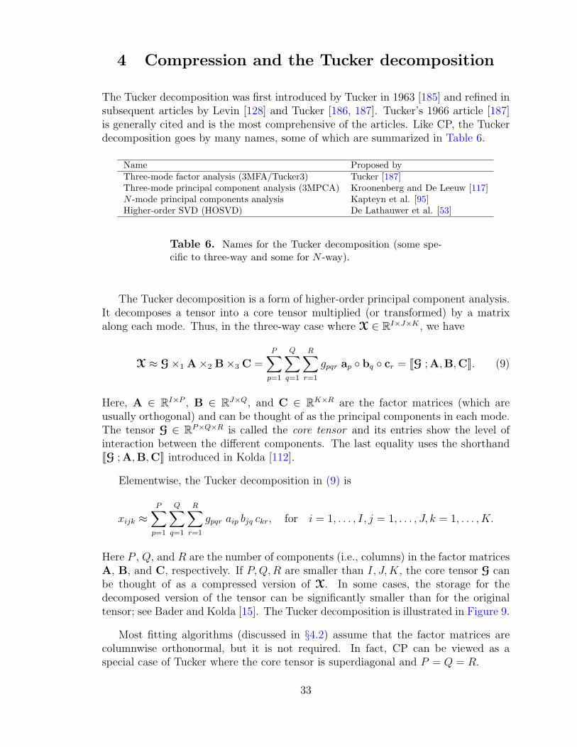
The Tucker decomposition is a form of higher-order principal component analysis.It decomposes a tensor into a core tensor multiplied (or transformed) by a matrixalong each mode. Thus, in the three-way case where X ∈ RI×J×K , we have

X ≈ G×1 A×2 B×3 C =P∑

p=1

Q∑q=1

R∑r=1

gpqr ap ◦ bq ◦ cr = JG ;A,B,CK. (9)

Here, A ∈ RI×P , B ∈ RJ×Q, and C ∈ RK×R are the factor matrices (which areusually orthogonal) and can be thought of as the principal components in each mode.The tensor G ∈ RP×Q×R is called the core tensor and its entries show the level ofinteraction between the different components. The last equality uses the shorthandJG ;A,B,CK introduced in Kolda [112].

Elementwise, the Tucker decomposition in (9) is

xijk ≈P∑

p=1

Q∑q=1

R∑r=1

gpqr aip bjq ckr, for i = 1, . . . , I, j = 1, . . . , J, k = 1, . . . , K.

Here P , Q, and R are the number of components (i.e., columns) in the factor matricesA, B, and C, respectively. If P, Q, R are smaller than I, J, K, the core tensor G canbe thought of as a compressed version of X. In some cases, the storage for thedecomposed version of the tensor can be significantly smaller than for the originaltensor; see Bader and Kolda [15]. The Tucker decomposition is illustrated in Figure 9.

Most fitting algorithms (discussed in §4.2) assume that the factor matrices arecolumnwise orthonormal, but it is not required. In fact, CP can be viewed as aspecial case of Tucker where the core tensor is superdiagonal and P = Q = R.

33

A

B

X =G

C

Figure 9. Tucker decomposition of a three-way array

The matricized versions of (9) are

X(1) ≈ AG(1)(C⊗B)T,

X(2) ≈ BG(2)(C⊗A)T,

X(3) ≈ CG(3)(B⊗A)T.

Though it was introduced in the context of three modes, the Tucker model canand has been generalized to N -way tensors [95] as:

X = G×1 A(1) ×2 A(2) · · · ×N A(N) = JG ;A(1),A(2), . . . ,A(N)K, (10)

or, elementwise, as

xi1i2···iN =

R1∑r1=1

R2∑r2=1

· · ·RN∑

rN=1

gr1r2···rNa

(1)i1r1

a(2)i2r2· · · a(N)

iNrN

for in = 1, . . . , In, n = 1, . . . , N.

The matricized version of (10) is

X(n) = A(n)G(n)(A(N) ⊗ · · · ⊗A(n+1) ⊗A(n−1) ⊗ · · · ⊗A(1))T.

Two important variations of the decomposition are also worth noting here. TheTucker2 decomposition [187] of a third-order array sets one of the factor matrices tobe the identity matrix. For instance, the Tucker2 decomposition is

X = G×1 A×2 B = JG ;A,B, IK.

This is the same as (9) except that G ∈ RP×Q×R with R = K and C = I, theK ×K identity matrix. Likewise, the Tucker1 decomposition [187] sets two of the

34

factor matrices to be the identity matrix. For example, if the second and third factormatrices are the identity matrix, then we have

X = G×1 A = JG ;A, I, IK.

This is equivalent to standard two-dimensional PCA since

X(1) = AG(1).

These concepts extend easily to the N -way case — we can set any subset of the factormatrices to the identity matrix.

4.1 The n-rank

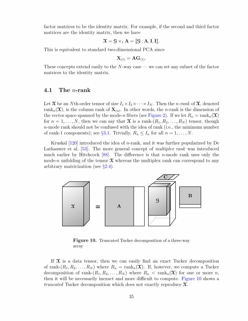
Let X be an Nth-order tensor of size I1×I2×· · ·×IN . Then the n-rank of X, denotedrankn(X), is the column rank of X(n). In other words, the n-rank is the dimension ofthe vector space spanned by the mode-n fibers (see Figure 2). If we let Rn = rankn(X)for n = 1, . . . , N , then we can say that X is a rank-(R1, R2, . . . , RN) tensor, thoughn-mode rank should not be confused with the idea of rank (i.e., the minimum numberof rank-1 components); see §3.1. Trivially, Rn ≤ In for all n = 1, . . . , N .

Kruskal [120] introduced the idea of n-rank, and it was further popularized by DeLathauwer et al. [53]. The more general concept of multiplex rank was introducedmuch earlier by Hitchcock [88]. The difference is that n-mode rank uses only themode-n unfolding of the tensor X whereas the multiplex rank can correspond to anyarbitrary matricization (see §2.4).

A

B

X =G

C

Figure 10. Truncated Tucker decomposition of a three-wayarray

If X is a data tensor, then we can easily find an exact Tucker decompositionof rank-(R1, R2, . . . , RN) where Rn = rankn(X). If, however, we compute a Tuckerdecomposition of rank-(R1, R2, . . . , RN) where Rn < rankn(X) for one or more n,then it will be necessarily inexact and more difficult to compute. Figure 10 shows atruncated Tucker decomposition which does not exactly reproduce X.

35

procedure HOSVD(X,R1,R2,. . . ,RN )for n = 1, . . . , N do

A(n) ← Rn leading left singular vectors of X(n)

end forG← X×1 A(1)T ×2 A(2)T · · · ×N A(N)T

return G,A(1),A(2), . . . ,A(N)

end procedure

Figure 11. Tucker’s “Method I” for computing a rank-(R1, R2, . . . , RN ) Tucker decomposition, later known as theHOSVD.

4.2 Computing the Tucker decomposition

In 1966, Tucker [187] introduced three methods for computing a Tucker decomposi-tion, but he was somewhat hampered by the computing ability of the day, statingthat calculating the eigendecomposition for a 300×300 matrix “may exceed computercapacity.” The first method in [187] is shown in Figure 11. The basic idea is to findthose components that best capture the variation in mode n, independent of the othermodes. Tucker presented it only for the three-way case, but the generalization to Nways is straightforward. This is sometimes referred to as the “Tucker1” method,though it is not clear whether this is because a Tucker1 factorization is computedfor each mode or it was Tucker’s first method. Today, this method is better knownas the higher-order SVD (HOSVD) from the work of De Lathauwer, De Moor, andVandewalle [53], who showed that the HOSVD is a convincing generalization of thematrix SVD and discussed ways to efficiently compute the singular vectors of X(n).When Rn < rankn(X) for one or more n, the decomposition is called the truncatedHOSVD.

The truncated HOSVD is not optimal, but it is a good starting point for aniterative alternating least squares (ALS) algorithm. In 1980, Kroonenberg and DeLeeuw [117] developed an ALS algorithm, called TUCKALS3, for computing a Tuckerdecomposition for three-way arrays. (They also had a variant called TUCKALS2 thatcomputed the Tucker2 decomposition of a three-way array.) Kapteyn, Neudecker, andWansbeek [95] later extended TUCKALS3 to N -way arrays for N > 3. De Lathauwer,De Moor, and Vandewalle [54] called it the Higher-order Orthogonal Iteration (HOOI);see Figure 12. If we assume that X is a tensor of size I1 × I2 × · · · × IN , then theoptimization problem that we wish to solve is

min∥∥∥X− JG ;A(1),A(2), . . . ,A(N)K

∥∥∥subject to G ∈ RR1×R2×···×RN

A(n) ∈ RIn×Rn and columnwise orthogonal for n = 1, . . . , N.

(11)

36

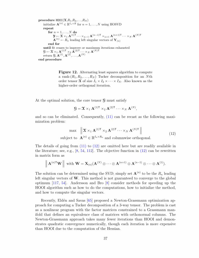
procedure HOOI(X,R1,R2,. . . ,RN )initialize A(n) ∈ RIn×R for n = 1, . . . , N using HOSVDrepeat

for n = 1, . . . , N doY← X×1 A(1)T · · · ×n−1 A(n−1)T ×n+1 A(n+1)T · · · ×N A(N)T

A(n) ← Rn leading left singular vectors of Y(n)

end foruntil fit ceases to improve or maximum iterations exhaustedG← X×1 A(1)T ×2 A(2)T · · · ×N A(N)T

return G,A(1),A(2), . . . ,A(N)

end procedure

Figure 12. Alternating least squares algorithm to computea rank-(R1, R2, . . . , RN ) Tucker decomposition for an Nthorder tensor X of size I1 × I2 × · · · × IN . Also known as thehigher-order orthogonal iteration.

At the optimal solution, the core tensor G must satisfy

G = X×1 A(1)T ×2 A(2)T · · · ×N A(N),

and so can be eliminated. Consequently, (11) can be recast as the following maxi-mization problem:

max∥∥∥X×1 A(1)T ×2 A(2)T · · · ×N A(N)T

∥∥∥subject to A(n) ∈ RIn×Rn and columnwise orthogonal.

(12)

The details of going from (11) to (12) are omitted here but are readily available inthe literature; see, e.g., [8, 54, 112]. The objective function in (12) can be rewrittenin matrix form as∥∥∥A(n)TW

∥∥∥ with W = X(n)(A(N) ⊗ · · · ⊗A(n+1) ⊗A(n−1) ⊗ · · · ⊗A(1)).

The solution can be determined using the SVD; simply set A(n) to be the Rn leadingleft singular vectors of W. This method is not guaranteed to converge to the globaloptimum [117, 54]. Andersson and Bro [8] consider methods for speeding up theHOOI algorithm such as how to do the computations, how to initialize the method,and how to compute the singular vectors.

Recently, Elden and Savas [65] proposed a Newton-Grassmann optimization ap-proach for computing a Tucker decomposition of a 3-way tensor. The problem is castas a nonlinear program with the factor matrices constrained to a Grassmann man-ifold that defines an equivalence class of matrices with orthonormal columns. TheNewton-Grassmann approach takes many fewer iterations than HOOI and demon-strates quadratic convergence numerically, though each iteration is more expensivethan HOOI due to the computation of the Hessian.

37

The question of how to choose the rank has been addressed by Kiers and Der Kinderen[102] who have a straightforward procedure (cf., CONCORDIA for CP in §3.4) forchoosing the appropriate rank of a Tucker model based on an HOSVD calculation.

4.3 Lack of uniqueness and methods to overcome it

Tucker decompositions are not unique. Consider the three-way decomposition in (9).Let U ∈ RP×P , V ∈ RQ×Q, and W ∈ RR×R be nonsingular matrices. Then

JG ;A,B,CK = JG×1 U×2 V ×3 W ;AU−1,BV−1,CW−1K.

In other words, we can modify the core G without affecting the fit so long as we applythe inverse modification to the factor matrices.

This freedom opens the door to choosing transformations that simplify the corestructure in some way so that most of the elements of G are zero, thereby eliminatinginteractions between corresponding components. Superdiagonalization of the core isimpossible, but it is possible to try to make as many elements zero or very small aspossible. This was first observed by Tucker [187] and has been studied by severalauthors; see, e.g., [85, 106, 146, 10]. One possibility is to apply a set of orthogonal ro-tations that optimizes a combination of orthomax functions on the core [99]. Anotheris to use a Jacobi-type algorithm to maximize the diagonal entries [137].

4.4 Applications of Tucker

Several examples of using the Tucker decomposition in chemical analysis are providedby Henrion [86] as part of a tutorial on N -way PCA. Examples from psychometrics areprovided by Kiers and Van Mechelen [108] in their overview of three-way componentanalysis techniques. The overview is a good introduction to three-way methods, ex-plaining when to use three-way techniques rather than two-way (based on an ANOVAtest), how to preprocess the data, guidance on choosing the rank of the decompositionand an appropriate rotation, and methods for presenting the results.

De Lathauwer and Vandewalle [57] consider applications of the Tucker decom-position to signal processing. Muti and Bourennane [147] have applied the Tuckerdecomposition to extend Wiener filters in signal processing.

Vasilescu and Terzopoulos [189] pioneered the use of Tucker decompositions incomputer vision with TensorFaces. They considered facial image data from multiplesubjects where each subject had multiple pictures taken under varying conditions.For instance, if the variation is the lighting, the data would be arranged into threemodes: person, lighting conditions, and pixels. Additional modes such as expression,camera angle, and more can also be incorporated. Recognition using TensorFaces

38

is significantly more accurate than standard PCA techniques [190]. TensorFaces isalso useful for compression and can remove irrelevant effects, such as lighting, whileretaining key facial features [191]. Wang and Ahuja [195, 196] used Tucker to modelfacial expressions and for image data compression, and Vlassic et al. [194] use Tuckerto transfer facial expressions.

Grigorascu and Regalia [72] consider extending ideas from structured matrices totensors. They are motivated by the structure in higher-order cumulants and cor-responding polyspectra in applications and develop an extensions of a Schur-typealgorithm.

In data mining, Savas and Elden [158, 159] applied the HOSVD to the problemof identifying handwritten digits. As mentioned previously, Acar et al. [3, 4], ap-plied different tensor decompositions, including Tucker, to the problem of discussiondetanglement in online chatrooms. J.-T. Sun et al. [172] used Tucker to analyzeweb site click-through data. Liu et al. [132] applied Tucker to create a tensor spacemodel, analogous to the well-known vector space model in text analysis. J. Sun et al.[170, 171] have written a pair of papers on dynamically updating a Tucker approxi-mation, with applications ranging from text analysis to environmental and networkmodeling.

39

This page intentionally left blank.

40

5 Other decompositions

There are a number of other tensor decompositions related to CP and Tucker. Most ofthese decompositions originated in the psychometrics and applied statistics communi-ties and have only recently become more widely known in fields such as chemometricsand social network analysis.

We list the decompositions discussed in this section in Table 7. We describethe decompositions in chronological order; for each decomposition, we survey itsorigins, briefly discuss computation, and describe some applications. We close outthis section with a discussion of nonnegative tensor decompositions and a few moredecompositions that are not covered in depth in this review.

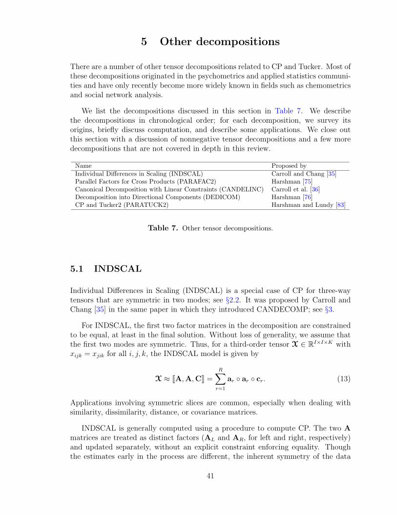
Name Proposed byIndividual Differences in Scaling (INDSCAL) Carroll and Chang [35]Parallel Factors for Cross Products (PARAFAC2) Harshman [75]Canonical Decomposition with Linear Constraints (CANDELINC) Carroll et al. [36]Decomposition into Directional Components (DEDICOM) Harshman [76]CP and Tucker2 (PARATUCK2) Harshman and Lundy [83]

Table 7. Other tensor decompositions.

5.1 INDSCAL

Individual Differences in Scaling (INDSCAL) is a special case of CP for three-waytensors that are symmetric in two modes; see §2.2. It was proposed by Carroll andChang [35] in the same paper in which they introduced CANDECOMP; see §3.

For INDSCAL, the first two factor matrices in the decomposition are constrainedto be equal, at least in the final solution. Without loss of generality, we assume thatthe first two modes are symmetric. Thus, for a third-order tensor X ∈ RI×I×K withxijk = xjik for all i, j, k, the INDSCAL model is given by

X ≈ JA,A,CK =R∑

r=1

ar ◦ ar ◦ cr. (13)

Applications involving symmetric slices are common, especially when dealing withsimilarity, dissimilarity, distance, or covariance matrices.

INDSCAL is generally computed using a procedure to compute CP. The two Amatrices are treated as distinct factors (AL and AR, for left and right, respectively)and updated separately, without an explicit constraint enforcing equality. Thoughthe estimates early in the process are different, the inherent symmetry of the data

41

causes the two factors to eventually converge, up to scaling by a diagonal matrix. Inother words,

AL = DAR,

AR = D−1AL,

where D is an R × R diagonal matrix. In practice, the last step is to set AL = AR

(or vice versa) and calculate C one last time [35]. If the iterates converge to a localminimum, there is no guarantee that the two factors will be related; see Ten Berge,Kiers, and De Leeuw [178].

Ten Berge, Sidiropoulos, and Rocci [180] have studied the typical and maximalrank of partially symmetric three-way tensors of size I × 2 × 2 and I × 3 × 3 (seeTable 5 in §3.1). The typical rank of these tensors is the same or smaller than thetypical rank of nonsymmetric tensors of the same size. Moreover, the CP solutionyields the INDSCAL solution whenever the CP solution is unique and, surprisingly,still does quite well even in the case of non-uniqueness. These results are restrictedto very specific cases, and Ten Berge et al. [180] note that much more general resultsare needed.

5.2 PARAFAC2

PARAFAC2 [75] is not strictly a tensor decomposition. Rather, it is a variant of CPthat can be applied to a collection of matrices that are equivalent in only one mode.In other words, it applies when we have K parallel matrices Xk, for k = 1, . . . , K,such that each Xk is of size Ik × J , where Ik is allowed to vary with k.

Essentially, PARAFAC2 relaxes some of CP’s constraints. Whereas CP is basedon a “parallel proportional profile principle” that applies the same factors across aparallel set of matrices, PARAFAC2 instead applies the same factor along one modeand allows the other factor matrix to vary. An advantage of PARAFAC2 is that, notonly can it approximate data in a regular three-way tensor with fewer constraintsthan CP, it can also be applied to a collection of matrices with varying sizes in onemode, e.g., same column dimension but different row size.

Let R be the number of dimensions of the decomposition. Then the PARAFAC2model has the following form:

Xk ≈ UkSkVT, k = 1, . . . , K. (14)

where Uk is an Ik × R matrix and Sk is a R × R diagonal matrix for k = 1, . . . , K,and V is a J ×R factor matrix that does not vary with k. The general PARAFAC2model for a collection of matrices with varying sizes is shown in Figure 13.

PARAFAC2 is not unique without additional constraints. For example, if T is an

42

Xk UkV

T=

Sk

Figure 13. Illustration of PARAFAC2.

R×R nonsingular matrix and Fk is an R×R diagonal matrix for k = 1, . . . , K, then

UkSkVT = (UkSkT

−1F−1k )Fk(VTT)T = GkFkW

T

is an equally valid decomposition. Consequently, to improve the uniqueness proper-ties, Harshman [75] imposed the constraint that the cross product UT

k Uk is constantover k, i.e., Φ = UT

k Uk for k = 1, . . . , K. Thus, with this constraint, PARAFAC2can be expressed as

Xk ≈ QkHSkVT, k = 1, . . . , K. (15)

Here, Uk = QkH where Qk is of size Ik × R and constrained to be orthonormal andH is an R × R matrix that does not vary by slice. The cross-product constraint isenforced implicitly since

UTk Uk = HTQT

k QkH = HTH = Φ.

5.2.1 Computing PARAFAC2

Algorithms for fitting PARAFAC2 either fit the cross-products of the covariance ma-trices [75, 97] (indirect fitting) or fit (15) to the original data itself [105] (direct fitting).The indirect fitting approach finds V, Sk and Φ corresponding to the cross products:

XTk Xk ≈ VSkΦSkV

T, k = 1, . . . , K.

This can be done by using a DEDICOM decomposition (see §5.4) with positive semi-definite constraints on Φ. The direct fitting approach solves for the unknowns in atwo-step iterative approach, first by finding Qk from a minimization using the SVDand then updating the remaining unknowns, H, Sk, and V, using one step of aCP-ALS procedure. See [105] for details.

PARAFAC2 is (essentially) unique under certain conditions pertaining to the num-ber of matrices (K), the positive definiteness of Φ, full column rank of A, and non-singularity of Sk [83, 176, 105].

43

5.2.2 PARAFAC2 applications

Bro et al. [28] use PARAFAC2 to handle time shifts in resolving chromatographic datawith spectral detection. In this application, the first mode corresponds to elution time,the second mode to wavelength, and the third mode to samples. The PARAFAC2model does not assume parallel proportional elution profiles but rather that the matrixof elution profiles preserves its “inner-product structure” across samples, which meansthat the cross-product of the corresponding factor matrices in PARAFAC2 is constantacross samples.

Wise, Gallager, and Martin [199] applied PARAFAC2 to the problem of faultdetection in a semi-conductor etch process. In this application (and many others),there is a difference in the number of time steps per batch. Alternative methods sucha time warping alter the original data. The advantage of PARAFAC2 is that it canbe used on the original data.

Chew et al. [40] use PARAFAC2 for clustering documents across multiple lan-guages. The idea is to extend the concept of latent semantic indexing [63, 61, 18]in a cross-language context by using multiple translations of the same collection ofdocuments, i.e., a parallel corpus. In this case, Xk is a term-by-document matrixfor the kth language in the parallel corpus. The number of terms varies considerablyby language. The resulting PARAFAC2 decomposition is such that the document-concept matrix V is the same across all languages, while each language has its ownterm-concept matrix Qk.

5.3 CANDELINC

A principal problem in multidimensional analysis is the interpretation of the fac-tors matrices from tensor decompositions. Consequently, including domain or userknowledge is desirable, and this can be done by imposing constraints. CANDELINC(canonical decomposition with linear constraints) is CP with linear constraints on oneor more of the factor matrices and was introduced by Carroll, Pruzansky, and Kruskal[36]. Though a constrained model may not explain as much variance in the data (i.e.,it may have a larger residual error), the decomposition is often more meaningful andinterpretable.

For instance, in the three-way case, CANDELINC requires that the CP factormatrices from (5) satisfy

A = ΦAA, B = ΦBB, C = ΦCC. (16)

Here, ΦA ∈ RI×M , ΦB ∈ RJ×N , and ΦC ∈ RK×P define the column space for eachfactor matrix. Thus, the CANDELINC model, (5) coupled with (16), is

X ≈ JΦAA,ΦBB,ΦCCK. (17)

44

Without loss of generality, the constraint matrices ΦA,ΦB,ΦC are assumed to beorthonormal. We can make this assumption because any matrix that does not satisfythe requirement can be replaced by one that generates the same column space and iscolumnwise orthogonal.

5.3.1 Computing CANDELINC

Fitting CANDELINC is straightforward. Under the assumption that the constraintmatrices are orthonormal, we can simply compute CP on the projected tensor. Forexample, in the third-order case discussed above, the projected M ×N × P tensor isgiven by

X = X×1 ΦTA ×2 ΦT

B ×3 ΦTC = JX ;ΦT

A,ΦTB,ΦT

CK.

We then compute its CP decomposition to get:

X ≈ JA, B, CK. (18)

The solution to the original problem is obtained by multiplying each factor matrix ofthe projected tensor by the corresponding constraint matrix as in (17).

5.3.2 CANDELINC and compression

If L � I, M � J , and N � K, then the projected tensor X is much smallerthan the original tensor X, and so decompositions of X are typically much faster.Indeed, CANDELINC is the theoretical base for compression [103, 27], which reducesthe original data to a more manageable size to provide a reasonable estimate of thefactors, which may optionally be refined with a few iterations of CP-ALS on theoriginal tensor. The utility of compression varies by application; Tomasi and Bro[184] report that compression does not necessarily lead to faster computational timesbecause more ALS iterations are required on the compressed tensor.

5.3.3 CANDELINC applications

As mentioned above, the primary application of CANDELINC is compressing large-scale data [103, 27]. Kiers developed a procedure involving compression and regu-larization to handle multicollinearity in chemometrics data [100]. Ibraghimov appliesCANDELINC-like ideas to develop preconditioners for 3D integral operators [90].

5.4 DEDICOM

DEDICOM (decomposition into directional components) is a family of decompositionsintroduced by Harshman [76]. The idea is as follows. Suppose that we have I objects

45

and a matrix X ∈ RI×I that describes the asymmetric relationships between them.For instance, the objects might be countries and xij represents the value of exportsfrom country i to country j. Typical factor analysis techniques either do not accountfor the fact that the two modes of a matrix may correspond to the same entitiesor that there may be directed interactions between them. DEDICOM, on the otherhand, attempts to group the I objects into R latent components (or groups) anddescribe their pattern of interactions by computing A ∈ RI×R and R ∈ RR×R suchthat

X ≈ ARAT. (19)

Each column in A corresponds to a latent component such that air indicates theparticipation of object i in group r. The matrix R indicates the interaction betweenthe different components, e.g., rij represents the exports from group i to group j.

There are two indeterminacies of scale and rotation that need to be addressed[76]. First, the columns of A may be scaled in a number of ways without affectingthe solution. One choice is to have unit length in the 2-norm; other choices give riseto different benefits of interpreting the results [78]. Second, the matrix A can betransformed with any nonsingular matrix T with no loss of fit to the data becauseARAT = (AT)(T−1RT−T)(AT)T. Thus, the solution obtained in A is not unique[78]. Nevertheless, it is standard practice to apply some accepted rotation to “fix” A.A common choice is to adopt VARIMAX rotation [94] such that the variance acrosscolumns of A is maximized.

A further practice in some problems is to ignore the diagonal entries of X inthe residual calculation [76]. For many cases, this makes sense because one wishesto ignore self-loops (e.g., a country does not export to itself). This is commonlyhandled by estimating the diagonal values from the current approximation ARAT

and including them in X.

Three-way DEDICOM [76] is a higher-order extension of the DEDICOM modelthat incorporates a third mode of the data. As with CP, adding a third dimen-sion gives this decomposition stronger uniqueness properties [83]. Here we assumeX ∈ RI×I×K . In our previous example of trade among nations, the third mode maycorrespond to time. For instance, k = 1 corresponds to trade in 1995, k = 2 to 1996,and so on. The decomposition is then

Xk ≈ ADkRDkAT for k = 1, . . . , K. (20)

Here A and R are as in (19), except that A is not necessarily orthogonal. Thematrices Dk ∈ RR×R are diagonal, and entry (Dk)rr indicates the participation ofthe rth latent component at time k. We can assemble the matrices Dk into a tensorD ∈ RR×R×K . Three-way DEDICOM is illustrated in Figure 14.

For many applications, it is reasonable to impose nonnegativity constraints onD [75]. Dual-domain DEDICOM is a variation where the scaling array D and/ormatrix A may be different on the left and right of R. This form is encapsulated byPARATUCK2 (see §5.5).

46

A

RD

X =D

AT

Figure 14. Three-way DEDICOM model.

5.4.1 Computing three-way DEDICOM

There are a number of algorithms for computing the two-way DEDICOM model, e.g.,[107], and for variations such as constrained DEDICOM [104, 156]. For three-wayDEDICOM, see Kiers [96, 97] and Bader, Harshman, and Kolda [13]. Because Aand D appear on both the left and right, fitting three-way DEDICOM is a difficultnonlinear optimization problem with many local minima.

Kiers [97] presents an alternating least squares (ALS) algorithm that is efficient onsmall tensors. Each column of A is updated with its own least-squares solution whileholding the others fixed. Each subproblem to compute one column of A involves afull eigendecomposition of a dense I×I matrix, which makes this procedure expensivefor large, sparse X. In a similar alternating fashion, the elements of D are updatedone at a time by minimizing a fourth degree polynomial. The best R for a given Aand D is found from a least-squares solution using the pseudo-inverse of an I2 × R2

matrix, which can be simplified to the inverse of an R2 ×R2 matrix.

Bader et al. [13] have proposed an algorithm called Alternating SimultaneousApproximation, Least Squares, and Newton (ASALSAN). The approach relies onthe same update for R as in [97] but uses different methods for updating A andD. Instead of solving for A column-wise, ASALSAN solves for all columns of Asimultaneously using an approximate least-squares solution. Because there are RKelements of D, which is not likely to be many, Newton’s method is used to find allelements of D simultaneously. The same paper [13] introduces a nonnegative variant.

5.4.2 DEDICOM applications

Most of the applications of DEDICOM in the literature have focused on two-way(matrix) data, but there are some three-way applications. Harshman and Lundy [82]analyzed asymmetric measures of yearly trade (import-export) among a set of nationsover a period of 10 years. Lundy et al. [135] presented an application of three-wayDEDICOM to skew-symmetric data for paired preference ratings of treatments forchronic back pain, though they note that they needed to impose some constraints to

47

A

BT

RD

A

DB

X =

Figure 15. General PARATUCK2 model.

get meaningful results.

Bader et al. [13] recently applied their ASALSAN method for computing DEDI-COM on email communication graphs over time. In this case, xijk corresponded tothe number of email messages sent from person i to person j in month k.

5.5 PARATUCK2

Harshman and Lundy [83] introduced PARATUCK2, a generalization of DEDICOMthat considers interactions between two possible different sets of objects. The nameis derived from the fact that this decomposition can be considered as a combinationof CP and TUCKER2.

Given a third-order tensor X ∈ RI×J×K , the goal is to group the mode-one objectsinto P latent components and the mode-two group into Q latent components. Thus,the PARATUCK2 decomposition is given by

Xk ≈ ADAk RDB

k BT, for k = 1, . . . , K. (21)

Here, A ∈ RI×P , B ∈ RJ×Q, R ∈ RP×Q, and DAk ∈ RP×P and DB

k ∈ RQ×Q arediagonal matrices. As with DEDICOM, the columns of A and B correspond to thelatent factors, so bjq is the association of object j with latent component q. Likewise,the entries of the diagonal matrices Dk indicate the degree of participation for eachlatent component with respect to the third dimension. Finally, the rectangular matrixR represents the interaction between the P latent components in A and the Q latentcomponents in B. The matrices DA

k and DBk can be stacked to form tensors DA and

DB respectively. PARATUCK2 is illustrated in Figure 15.

Harshman and Lundy [83] prove the uniqueness of axis orientation for the generalPARATUCK2 model and for the symmetrically weighted version (i.e., where DA =DB), all subject to the conditions that P = Q and R has no zeros.

48

5.5.1 Computing PARATUCK2

Bro [25] discusses an alternating least-squares algorithm for computing the parametersof PARATUCK2. The algorithm follows in the same spirit as Kiers’ DEDICOMalgorithm [97] except that the problem is only linear in the parameters A, DA,B, DB,and R and involves only linear least-squares subproblems.

5.5.2 PARATUCK2 applications

Harshman and Lundy [83] proposed PARATUCK2 as a general model for a numberof existing models, including PARAFAC2 (see §5.2) and three-way DEDICOM (see§5.4). Consequently, there are few published applications of PARATUCK2 proper.

Bro [25] mentions that PARATUCK2 is appropriate for problems that involveinteractions between factors or when more flexibility is needed than CP but not asmuch as Tucker. This can occur, for example, with rank-deficient data in physicalchemistry, for which a slightly restricted form of PARATUCK2 is suitable. Bro [25]cites an example of the spectrofluorometric analysis of three types of cow’s milk. Twoof the three components are almost collinear, which means that CP would be unstableand could not identify the three components. A rank-(2, 3, 3) analysis with a Tuckermodel is possible but would introduce rotational indeterminacy. A restricted form ofPARATUCK2, with two columns in A and three in B, is appropriate in this case.

5.6 Nonnegative tensor factorizations

Paatero and Tapper [151] and Lee and Seung [126] proposed using nonnegative ma-trix factorizations for analyzing nonnegative data, such as environmental models andgrayscale images, because it is desirable for the decompositions to retain the nonneg-ative characteristics of the original data and thereby facilitate easier interpretation.It is also natural to impose nonnegativity constraints on tensor factorizations. Manypapers refer to nonnegative tensor factorization generically as NTF but fail to dif-ferentiate between CP and Tucker. In the sequel, we use the terminology NNCP(nonnegative CP) and NNT (nonnegative Tucker).

Bro and De Jong [29] consider NNCP and NNT. They solve the subproblems inCP-ALS and Tucker-ALS with a specially adapted version of the NNLS method ofLawson and Hanson [125]. In the case of NNCP for a third-order tensor, subproblem(8) requires a least squares solution for A. The change here is to impose nonnegativityconstraints on A.

Similarly, for NNCP, Friedlander and Hatz [68] solve a bound constrained linearleast-squares problem. Additionally, they impose sparseness constraints by regular-izing the nonnegative tensor factorization with an l1-norm penalty function. While

49

this function is nondifferentiable, it has the effect of “pushing small values exactlyto zero while leaving large (and significant) entries relatively undisturbed.” Whilethe solution of the standard problem is unbounded due to the indeterminacy of scale,regularizing the problem has the added benefit of keeping the solution bounded. Theydemonstrate the effectiveness of their approach on image data.

Paatero [148] uses a Gauss-Newton method with a logarithmic penalty functionto enforce the nonnegativity constraints in NNCP. The implementation is describedin [149].

Welling and Weber [197] do multiplicative updates like Lee and Seung [126] forNNCP. For instance, the update for A in third-order NNCP is given by:

air ← air

(X(1)Z)ir

(AZTZ)ir

, where Z = (C�B).

It is helpful to add a small number like ε = 10−9 to the denominator to add stabilityto the calculation and guard against introducing a negative number from numericalunderflow. Welling and Weber’s application is to image decompositions. FitzGerald,Cranitch, and Coyle [67] use a multiplicative update form of NNCP for sound sourceseparation. Bader, Berry, and Browne [12] apply NNCP using multiplicative updatesto discussion tracking in Enron email data. Mørup, Hansen, Parnas, and Arnfred [141]also develop a multiplicative update for NNCP. They consider both least squares andKulbach-Leibler (KL) divergence, and the methods are applied to EEG data.

Shashua and Hazan [161] derive an EM-based method to calculate a rank-oneNNCP decomposition. A rank-R NNCP model is calculated by doing a series ofrank-one approximations to the residual. They apply the method to problems incomputer vision. Hazan, Polak, and Shashua [84] apply the method to image dataand observe that treating a set of images as a third-order tensor is better in termsof handling spatial redundancy in images, as opposed to using nonnegative matrixfactorizations on a matrix of vectorized images.

Mørup, Hansen, and Arnfred [142] develop multiplicative updates for a NNT de-composition and impose sparseness constraints to enhance uniqueness. Moreover,they observe that structure constraints can be imposed on the core tensor (to repre-sent known interactions) and the factor matrices (per desired structure). They applyNNT with sparseness constraints to EEG data.

Bader, Harshman, and Kolda [13] imposed nonnegativity constraints on the DEDI-COM model using a nonnegative version of the ASALSAN method. They replacedthe least squares updates with the multiplicative update introduced in [126]. TheNewton procedure for updating D already employed nonnegativity constraints.

50

5.7 More decompositions

Recently, several different groups of researchers have proposed models that combineaspects of CP and Tucker. Recall that CP expresses a tensor as the sum of rank-onetensors. In these newer models, the tensor is expressed as a sum of low-rank Tuckertensors. In other words, for a third-order tensor X ∈ RI×J×K , we have

X =R∑

r=1

JGr ;Ar,Br,CrK.

Here we assume Gr is of size Mr×Nr×Pr, Ar is of size I×Mr, Br is of size J×Nr, andCr is of size K × Pr, for r = 1, . . . , R. Figure 16 shows an example. Bro, Harshman,and Sidiropoulos [30, 5] propose the PARALIND model that allows some modes inCP to interact. De Almeida, Favier, and Mota [46] give an overview of some aspectsof these models and their application to problems in blind beamforming and multi-antenna coding. In a series of papers, De Lathauwer [49, 50] and De Lathauwer andNion [56] explore a general class of such decompositions, their uniqueness properties,and computational algorithms.

B1

X =

G1

C1

+ +A1...

BRGR

AR

CR

Figure 16. Block decomposition of a third-order tensor.

Mahoney et al. [136] extend the matrix CUR decomposition to tensors; othershave done related work using sampling methods for tensor approximation [62, 47].

Both De Lathauwer et al. [52] and Vasilescu and Terzopoulos [192] have exploredhigher-order versions of independent component analysis (ICA), a variation of PCAthat does not require orthogonal components. Beckmann and Smith [17] extend CPto develop a probabilistic ICA. Bro, Sidiropoulos and Smilde [32] and Vega-Montotoand Wentzell [193] formulate maximum-likelihood versions of CP.

Acar and Yener [5] discuss several of these decompositions as well as some notcovered here: shifted CP and Tucker [80] and convoluted CP [145].

51

This page intentionally left blank.

52

6 Software for tensors

The earliest consideration of tensor computation issues dates back to 1973 whenPereyra and Scherer [152] considered basic operations in tensor spaces and how toprogram them. But general-purpose software for working with tensors has only be-come readily available in the last decade. In this section, we survey the softwareavailable for working with tensors.

MATLAB, Mathematica, and Maple all have support for tensors. MATLAB in-troduced support for dense multidimensional arrays in version 5.0 (released in 1997).MATLAB supports elementwise manipulation on tensors. More general operationsand support for sparse and structured tensors are provided by external toolboxes(N-way, CuBatch, PLS Toolbox, Tensor Toolbox), discussed below. Mathematicasupports tensors, and there is a Mathematica package for working with tensors thataccompanies Ruız-Tolosa and Castillo [157]. In terms of sparse tensors, Mathemat-ica 6.0 stores its SparseArray’s as Lists.4 Maple has the capacity to work withsparse tensors using the array command and supports mathematical operations formanipulating tensors that arise in the context of physics and general relativity.

The N-way Toolbox for MATLAB, by Andersson and Bro [9], provides a largecollection of algorithms for computing different tensor decompositions. It providesmethods for computing CP and Tucker, as well as many of the other models such asmultilinear partial least squares (PLS). Additionally, many of the methods can handleconstraints (e.g., nonnegativity) and missing data. CuBatch [70] is a graphical userinterface in MATLAB for the analysis of data that is built on top of the N-wayToolbox. Its focus is data centric, offering an environment for preprocessing datathrough diagnostic assessment, such as jack-knifing and bootstrapping. The interfaceallows custom extensions through an open architecture. Both the N-way Toolbox andCuBatch are freely available.

The commercial PLS Toolbox for MATLAB [198] also provides a number of multi-dimensional models, including CP and Tucker, with an emphasis towards data analy-sis in chemometrics. Like the N-way Toolbox, the PLS Toolbox can handle constraintsand missing data.

The Tensor Toolbox for MATLAB, by Bader and Kolda [14, 15, 16], is a generalpurpose set of classes that extends MATLAB’s core capabilities to support operationssuch as tensor multiplication and matricization. It comes with ALS-based algorithmsfor CP and Tucker, but the goal is to enable users to easily develop their own al-gorithms. The Tensor Toolbox is unique in its support for sparse tensors, which itstores in coordinate format. Other recommendations for storing sparse tensors havebeen made; see [131, 130]. The Tensor Toolbox also supports structured tensors sothat it can store and manipulate, e.g., a CP representation of a large-scale sparsetensor. The Tensor Toolbox is freely available for research and evaluation purposes.

4Visit the Mathematica web site (www.wolfram.com) and search on “Tensors”.

53

The Multilinear Engine by Paatero [149] is a FORTRAN code based on the con-jugate gradient algorithm that also computes a variety of multilinear models. Itsupports CP, PARAFAC2, and more.

There are also some packages in C++. The HUJI Tensor Library (HTL) by Zass[201] is a C++ library of classes for tensors, including support for sparse tensors. HTLdoes not support tensor multiplication, but it does support inner product, addition,elementwise multiplication, etc. FTensor, by Landry [123], is a collection of template-based tensor classes in C++ for general relativity applications; it supports functionssuch as binary operations and internal and external contractions. The tensors areassumed to be dense, though symmetries are exploited to optimize storage. TheBoost Multidimensional Array Library (Boost.MultiArray) [69] provides a C++ classtemplate for multidimensional arrays that is efficient and convenient for expressingdense N -dimensional arrays. These arrays may be accessed using a familiar syntax ofnative C++ arrays, but it does not have key mathematical concepts for multilinearalgebra, such as tensor multiplication.

54

7 Discussion

This survey has provided an overview of tensor decompositions and their applications.The primary focus was on the CP and Tucker decompositions, but we have alsopresented some of the other models such as PARAFAC2. There is a flurry of currentresearch on more efficient methods for computing tensor decompositions and bettermethods for determining typical and maximal tensor ranks.

We have mentioned applications ranging from psychometrics and chemometricsto computer visualization and data mining, but many more applications of tensorsare being developed. For instance, in mathematics, Grasedyck [71] uses the ten-sor structure in finite element computations to generate low-rank Kronecker prod-uct approximations. As another example, Lim [129] (see also Qi [153]) discusseshigher-order extensions of singular values and eigenvalues. For supersymmetric ten-sor X ∈ RI×I×···×I or order N , the scalar λ is an eigenvalue and the vector v ∈ RI itscorresponding eigenvector if

X •2 x •3 x · · · •N x = λx.

No doubt more applications, both inside and outside of mathematics, will find usesfor tensor decompositions in the future.

Thus far, most computational work is done in MATLAB and all is serial. In thefuture, there will be a need for libraries that take advantage of parallel processorsand/or multi-core architectures. Numerous data-centric issues exist as well, such aspreparing the data for processing; see, e.g., [33]. Another problem is missing data,especially systematically missing data, is issue in chemometrics; see Tomasi and Bro[183] and references therein. For a general discussion on handling missing data, seeKiers [98].

55

References

[1] E. Acar, C. A. Bingol, H. Bingol, R. Bro, and B. Yener, Multiwayanalysis of epilepsy tensors, Bioinformatics, 23 (2007), pp. i10–i18.

[2] , Seizure recognition on epilepsy feature tensor, in Proceedings of the 29thInternational Conference of IEEE Engineering in Medicine and Biology Society,2007. To appear.

[3] E. Acar, S. A. Camtepe, M. S. Krishnamoorthy, and B. Yener,Modeling and multiway analysis of chatroom tensors, in ISI 2005: IEEE In-ternational Conference on Intelligence and Security Informatics, vol. 3495 ofLecture Notes in Computer Science, Springer, 2005, pp. 256–268.

[4] E. Acar, S. A. Camtepe, and B. Yener, Collective sampling and analysisof high order tensors for chatroom communications, in ISI 2006: IEEE Interna-tional Conference on Intelligence and Security Informatics, vol. 3975 of LectureNotes in Computer Science, Berlin, 2006, Springer, pp. 213–224.

[5] E. Acar and B. Yener, Unsupervised multiway data analysis: a litera-ture survey. Submitted for publication. Available at http://www.cs.rpi.edu/research/pdf/07-06.pdf, 2007.

[6] J. Alexander and A. Hirschowitz, Polynomical interpolation in severalvariables, J. Algebraic Geom., 1995 (1995), pp. 201–222. Cited in [43].

[7] C. M. Andersen and R. Bro, Practical aspects of PARAFAC modeling offluorescence excitation-emission data, J. Chemometr., 17 (2003), pp. 200–215.

[8] C. A. Andersson and R. Bro, Improving the speed of multi-way algorithms:Part I. Tucker3, Chemometr. Intell. Lab., 42 (1998), pp. 93–103.

[9] C. A. Andersson and R. Bro, The N-way toolbox for MATLAB,Chemometr. Intell. Lab., 52 (2000), pp. 1–4. See also http://www.models.

kvl.dk/source/nwaytoolbox/.

[10] C. A. Andersson and R. Henrion, A general algorithm for obtaining simplestructure of core arrays in N-way PCA with application to fluorimetric data,Comput. Stat. Data. An., 31 (1999), pp. 255–278.

[11] C. J. Appellof and E. R. Davidson, Strategies for analyzing data fromvideo fluorometric monitoring of liquid chromatographic effluents, Anal. Chem.,53 (1981), pp. 2053–2056.

[12] B. W. Bader, M. W. Berry, and M. Browne, Discussion tracking inEnron email using PARAFAC. Text Mining Workshop, Apr. 2007.

56

[13] B. W. Bader, R. A. Harshman, and T. G. Kolda, Temporal analysis ofsemantic graphs using ASALSAN, in ICDM 2007: Proceedings of the 7th IEEEInternational Conference on Data Mining, 2007. To appear.

[14] B. W. Bader and T. G. Kolda, Algorithm 862: MATLAB tensor classesfor fast algorithm prototyping, ACM T. Math. Software, 32 (2006), pp. 635–653.

[15] , Efficient MATLAB computations with sparse and factored tensors, SIAMJournal on Scientific Computing, (2007). Accepted.

[16] , MATLAB tensor toolbox, version 2.2. http://csmr.ca.sandia.gov/

~tgkolda/TensorToolbox/, January 2007.

[17] C. Beckmann and S. Smith, Tensorial extensions of independent componentanalysis for multisubject FMRI analysis, NeuroImage, 25 (2005), pp. 294–311.

[18] M. W. Berry, S. T. Dumais, and G. W. O’Brien, Using linear algebrafor intelligent information retrieval, SIAM Rev., 37 (1995), pp. 573–595.

[19] G. Beylkin and M. J. Mohlenkamp, Numerical operator calculus in higherdimensions, P. Natl. Acad. Sci., 99 (2002), pp. 10246–10251.

[20] , Algorithms for numerical analysis in high dimensions, SIAM J. Sci. Com-put., 26 (2005), pp. 2133–2159.

[21] D. Bini, The role of tensor rank in the complexity analysis of bilinear forms.Presentation at ICIAM07, Zurich, Switzerland, July 2007.

[22] D. Bini, M. Capovani, G. Lotti, and F. Romani, o(n2.7799) complexityfor n × n approximate matrix multiplication, Inform. Process. Lett., 8 (1979),pp. 234–235.

[23] M. Blaser, On the complexity of the multiplication of matrices in small for-mats, J. Complexity, 19 (2003), pp. 43–60. Cited in [21].

[24] R. Bro, PARAFAC. Tutorial and applications, Chemometr. Intell. Lab., 38(1997), pp. 149–171.

[25] , Multi-way analysis in the food industry: Models, algorithms, and ap-plications, PhD thesis, University of Amsterdam, 1998. Available at http:

//www.models.kvl.dk/research/theses/.

[26] , Review on multiway analysis in chemistry — 2000–2005, Critical Reviewsin Analytical Chemistry, 36 (2006), pp. 279–293.

[27] R. Bro and C. A. Andersson, Improving the speed of multi-way algorithms:Part II. Compression, Chemometr. Intell. Lab., 42 (1998), pp. 105–113.

57

[28] R. Bro, C. A. Andersson, and H. A. L. Kiers, PARAFAC2—Part II.Modeling chromatographic data with retention time shifts, J. Chemometr., 13(1999), pp. 295–309.

[29] R. Bro and S. De Jong, A fast non-negativity-constrained least squaresalgorithm, J. Chemometr., 11 (1997), pp. 393–401.

[30] R. Bro, R. A. Harshman, and N. D. Sidiropoulos, Modeling multi-way data with linearly dependent loadings, Tech. Report 2005-176, KVL, 2005.Cited in [5]. Available at http://www.telecom.tuc.gr/~nikos/paralind_

KVLTechnicalReport2005-176.pdf.

[31] R. Bro and H. A. L. Kiers, A new efficient method for determining the num-ber of components in PARAFAC models, J. Chemometr., 17 (2003), pp. 274–286.

[32] R. Bro, N. Sidiropoulos, and A. Smilde, Maximum likelihood fitting usingordinary least squares algorithms, J. Chemometr., 16 (2002), pp. 387–400.

[33] R. Bro and A. K. Smilde, Centering and scaling in component analysis,Psychometrika, 17 (2003), pp. 16–33.

[34] N. Bshouty, Maximal rank of m× n× (mn− k) tensors, SIAM J. Comput.,19 (1990), pp. 467–471.

[35] J. D. Carroll and J. J. Chang, Analysis of individual differences in mul-tidimensional scaling via an N-way generalization of ‘Eckart-Young’ decompo-sition, Psychometrika, 35 (1970), pp. 283–319.

[36] J. D. Carroll, S. Pruzansky, and J. B. Kruskal, CANDELINC: Ageneral approach to multidimensional analysis of many-way arrays with linearconstraints on parameters, Psychometrika, 45 (1980), pp. 3–24.

[37] R. B. Cattell, Parallel proportional profiles and other principles for deter-mining the choice of factors by rotation, Psychometrika, 9 (1944), pp. 267–283.

[38] R. B. Cattell, The three basic factor-analytic research designs — their in-terrelations and derivatives, Psychological Bulletin, 49 (1952), pp. 499–452.

[39] B. Chen, A. Petropolu, and L. De Lathauwer, Blind identificationof convolutive MIMO systems with 3 sources and 2 sensors, Applied SignalProcessing, (2002), pp. 487–496. (Special Issue on Space-Time Coding and ItsApplications, Part II).

[40] P. A. Chew, B. W. Bader, T. G. Kolda, and A. Abdelali, Cross-language information retrieval using PARAFAC2, in KDD ’07: Proceedings ofthe 13th ACM SIGKDD International Conference on Knowledge Discovery andData Mining, ACM Press, 2007, pp. 143–152.

58

[41] P. Comon, Tensor decompositions: State of the art and applications, in Mathe-matics in Signal Processing V, J. G. McWhirter and I. K. Proudler, eds., OxfordUniversity Press, 2001, pp. 1–24.

[42] P. Comon, Canonical tensor decompositions, I3S Report RR-2004-17, Lab.I3S, 2000 route des Lucioles, B.P.121,F-06903 Sophia-Antipolis cedex, France,June 17 2004.

[43] P. Comon, G. Golub, L.-H. Lim, and B. Mourrain, Symmetric tensorsand symmetric tensor rank, SCCM Technical Report 06-02, Stanford University,2006.

[44] P. Comon, J. M. F. Ten Berge, L. De Lathauwer, and J. Castaing,Generic and typical ranks of multi-way arrays. Submitted for publication, 2007.

[45] R. Coppi and S. Bolasco, eds., Multiway Data Analysis, North-Holland,Amsterdam, 1989.

[46] A. De Almeida, G. Favier, and J. ao Mota, The constrained block-PARAFAC decomposition. Presented at TRICAP2006, Chania, Greece.Available online at http://www.telecom.tuc.gr/~nikos/TRICAP2006main/

TRICAP2006_Almeida.pdf, June 2006.

[47] W. F. de la Vega, M. Karpinski, R. Kannan, and S. Vempala, Tensordecomposition and approximation schemes for constraint satisfaction problems,in STOC ’05: Proceedings of the Thirty-Seventh Annual ACM Symposium onTheory of Computing, ACM Press, 2005, pp. 747–754.

[48] L. De Lathauwer, A link between the canonical decomposition in multilinearalgebra and simultaneous matrix diagonalization, SIAM J. Matrix Anal. A., 28(2006), pp. 642–666.

[49] , Decompositions of a higher-order tensor in block terms — Part I: Lemmasfor partitioned matrices. Submitted for publication, 2007.

[50] , Decompositions of a higher-order tensor in block terms — Part II: Defi-nitions and uniqueness. Submitted for publication, 2007.

[51] L. De Lathauwer and B. De Moor, From matrix to tensor: Multilinear al-gebra and signal processing, Tech. Report ESAT-SISTA/TR 1997-58, KatholiekeUniversiteit Leuven, 1997.

[52] L. De Lathauwer, B. De Moor, and J. Vandewalle, An introductionto independent component analysis, J. Chemometr., 14 (2000), pp. 123 – 149.

[53] , A multilinear singular value decomposition, SIAM J. Matrix Anal. A., 21(2000), pp. 1253–1278.

59

[54] , On the best rank-1 and rank-(R1, R2, . . . , RN) approximation of higher-order tensors, SIAM J. Matrix Anal. A., 21 (2000), pp. 1324–1342.

[55] , Computation of the canonical decomposition by means of a simultaneousgeneralized Schur decomposition, SIAM J. Matrix Anal. A., 26 (2004), pp. 295–327.

[56] L. De Lathauwer and D. Nion, Decompositions of a higher-order tensorin block terms — Part III: Alternating least squares algorithms. Submitted forpublication, 2007.

[57] L. De Lathauwer and J. Vandewalle, Dimensionality reduction in higher-order signal processing and rank-(R1, R2, . . . , RN) reduction in multilinear alge-bra, Linear Algebra Appl., 391 (2004), pp. 31 – 55.

[58] V. de Silva and L.-H. Lim, Tensor rank and the ill-posedness of the bestlow-rank approximation problem, SCCM Technical Report 06-06, Stanford Un-viersity, 2006.

[59] , Tensor rank and the ill-posedness of the best low-rank approximation prob-lem, SIAM Journal on Matrix Analysis and Applications, (2006). To appear.

[60] M. De Vos, A. Vergult, L. De Lathauwer, W. De Clercq,S. Van Huffel, P. Dupont, A. Palmini, and W. Van Paesschen,Canonical decomposition of ictal scalp EEG reliably detects the seizure onsetzone, NeuroImage, 37 (2007), pp. 844–854.

[61] S. C. Deerwester, S. T. Dumais, T. K. Landauer, G. W. Furnas, andR. A. Harshman, Indexing by latent semantic analysis, J. Am. Soc. Inform.Sci., 41 (1990), pp. 391–407.

[62] P. Drineas and M. W. Mahoney, A randomized algorithm for a tensor-based generalization of the singular value decomposition, Linear Algebra Appl.,420 (2007), pp. 553–571.

[63] S. T. Dumais, G. W. Furnas, T. K. Landauer, S. Deerwester, andR. Harshman, Using latent semantic analysis to improve access to textualinformation, in CHI ’88: Proceedings of the SIGCHI Conference on FumanFactors in Computing Systems, ACM Press, 1988, pp. 281–285.

[64] G. Eckart and G. Young, The approximation of one matrix by another oflower rank, Psychometrika, 1 (1936), pp. 211–218.

[65] L. Elden and B. Savas, A Newton–Grassmann method for computing thebest multi-linear rank-(r1, r2, r3) approximation of a tensor, Tech. Report LITH-MAT-R-2007-6-SE, Department of Mathematics, Linkopings Universitet, 2007.

60

[66] N. K. M. Faber, R. Bro, and P. K. Hopke, Recent developments inCANDECOMP/PARAFAC algorithms: A critical review, Chemometr. Intell.Lab., 65 (2003), pp. 119–137.

[67] D. FitzGerald, M. Cranitch, and E. Coyle, Non-negative tensor fac-torisation for sound source separation, in ISSC 2005: Proceedings of the IrishSignals and Systems Conference, 2005.

[68] M. P. Friedlander and K. Hatz, Computing nonnegative tensor factoriza-tions, Tech. Report TR-2006-21, Department of Computer Science, Universityof British Columbia, Oct. 2006.

[69] R. Garcia and A. Lumsdaine, MultiArray: A C++ library for generic pro-gramming with arrays, Software: Practice and Experience, 35 (2004), pp. 159–188.

[70] S. Gourvenec, G. Tomasi, C. Durville, E. Di Crescenzo, C. Saby,D. Massart, R. Bro, and G. Oppenheim, CuBatch, a MATLAB Interfacefor n-mode Data Analysis, Chemometr. Intell. Lab., 77 (2005), pp. 122–130.

[71] L. Grasedyck, Existence and computation of low Kronecker-rank approxima-tions for large linear systems of tensor product structure, Computing, 72 (2004),pp. 247–265.

[72] V. S. Grigorascu and P. A. Regalia, Tensor displacement structures andpolyspectral matching, in Fast Reliable Algorithms for Matrices with Structure,T. Kaliath and A. H. Sayed, eds., SIAM, Philadelphia, 1999, pp. 245–276.

[73] R. A. Harshman, Foundations of the PARAFAC procedure: Models and con-ditions for an “explanatory” multi-modal factor analysis, UCLA Working Pa-pers in Phonetics, 16 (1970), pp. 1–84. Available at http://publish.uwo.ca/

~harshman/wpppfac0.pdf.

[74] , Determination and proof of minimum uniqueness conditions forPARAFAC, UCLA Working Papers in Phonetics, 22 (1972), pp. 111–117. Avail-able from http://publish.uwo.ca/~harshman/wpppfac1.pdf.

[75] , PARAFAC2: Mathematical and technical notes, UCLA Working Papersin Phonetics, 22 (1972), pp. 30–47.

[76] , Models for analysis of asymmetrical relationships among n objects or stim-uli, in First Joint Meeting of the Psychometric Society and the Society forMathematical Psychology, McMaster University, Hamilton, Ontario, August1978. Available at http://publish.uwo.ca/~harshman/asym1978.pdf.

[77] , An index formulism that generalizes the capabilities of matrix notationand algebra to n-way arrays, J. Chemometr., 15 (2001), pp. 689–714.

61

[78] R. A. Harshman, P. E. Green, Y. Wind, and M. E. Lundy, A model forthe analysis of asymmetric data in marketing research, Market. Sci., 1 (1982),pp. 205–242.

[79] R. A. Harshman and S. Hong, ‘Stretch’ vs. ‘slice’ methods for representingthree-way structure via matrix notation, J. Chemometr., 16 (2002), pp. 198–205.

[80] R. A. Harshman, S. Hong, and M. E. Lundy, Shifted factor analysis-PartI: Models and properties, J. Chemometr., 17 (2003), pp. 363–378. Cited in [5].

[81] R. A. Harshman and M. E. Lundy, Data preprocessing and the extendedPARAFAC model, in Research Methods for Multi-mode Data Analysis, H. G.Law, C. W. Snyder, J. Hattie, and R. K. McDonald, eds., Praeger Publishers,New York, 1984, pp. 216–284.

[82] R. A. Harshman and M. E. Lundy, Three-way DEDICOM: Analyzing mul-tiple matrices of asymmetric relationships. Paper presented at the Annual Meet-ing of the North American Psychometric Society, 1992.

[83] R. A. Harshman and M. E. Lundy, Uniqueness proof for a fam-ily of models sharing features of Tucker’s three-mode factor analysis andPARAFAC/CANDECOMP, Psychometrika, 61 (1996), pp. 133–154.

[84] T. Hazan, S. Polak, and A. Shashua, Sparse image coding using a 3Dnon-negative tensor factorization, in ICCV 2005: 10th IEEE International Con-ference on Computer Vision, vol. 1, IEEE Computer Society, 2005, pp. 50–57.

[85] R. Henrion, Body diagonalization of core matrices in three-way principal com-ponents analysis: Theoretical bounds and simulation, J. Chemometr., 7 (1993),pp. 477–494.

[86] , N-way principal component analysis theory, algorithms and applications,Chemometr. Intell. Lab., 25 (1994), pp. 1–23.

[87] F. L. Hitchcock, The expression of a tensor or a polyadic as a sum of prod-ucts, J. Math. Phys. Camb., 6 (1927), pp. 164–189.

[88] , Multilple invariants and generalized rank of a p-way matrix or tensor, J.Math. Phys. Camb., 7 (1927), pp. 39–70.

[89] T. D. Howell, Global properties of tensor rank, Linear Algebra Appl., 22(1978), pp. 9–23.

[90] I. Ibraghimov, Application of the three-way decomposition for matrix com-pression, Numer. Linear Algebr., 9 (2002), pp. 551–565.

[91] J. JaJa, Optimal evaluation of pairs of bilinear forms, SIAM J. Comput., 8(1979), pp. 443–462.

62

[92] J. Jiang, H. Wu, Y. Li, and R. Yu, Three-way data resolution by alternatingslice-wise diagonalization (ASD) method, J. Chemometr., 14 (2000), pp. 15–36.

[93] T. Jiang and N. Sidiropoulos, Kruskal’s permutation lemma and the iden-tification of CANDECOMP/PARAFAC and bilinear models with constant mod-ulus constraints, IEEE T. Signal Proces., 52 (2004), pp. 2625–2636.

[94] H. Kaiser, The varimax criterion for analytic rotation in factor analysis, Psy-chometrika, 23 (1958), pp. 187–200.

[95] A. Kapteyn, H. Neudecker, and T. Wansbeek, An approach to n-modecomponents analysis, Psychometrika, 51 (1986), pp. 269–275.

[96] H. A. L. Kiers, An alternating least squares algorithm for fitting the two-and three-way DEDICOM model and the IDIOSCAL model, Psychometrika, 54(1989), pp. 515–521.

[97] , An alternating least squares algorithm for PARAFAC2 and three-wayDEDICOM, Comput. Stat. Data. An., 16 (1993), pp. 103–118.

[98] , Weighted least squares fitting using ordinary least squares algorithms, Psy-chometrika, 62 (1997), pp. 215–266.

[99] , Joint orthomax rotation of the core and component matrices resulting fromthree-mode principal components analysis, J. Classif., 15 (1998), pp. 245 – 263.

[100] , A three-step algorithm for CANDECOMP/PARAFAC analysis of largedata sets with multicollinearity, J. Chemometr., 12 (1998), pp. 255–171.

[101] , Towards a standardized notation and terminology in multiway analysis, J.Chemometr., 14 (2000), pp. 105–122.

[102] H. A. L. Kiers and A. Der Kinderen, A fast method for choosing thenumbers of components in Tucker3 analysis, Brit. J. Math. Stat. Psy., 56 (2003),pp. 119–125.

[103] H. A. L. Kiers and R. A. Harshman, Relating two proposed methods forspeedup of algorithms for fitting two- and three-way principal component andrelated multilinear models, Chemometr. Intell. Lab., 36 (1997), pp. 31–40.

[104] H. A. L. Kiers and Y. Takane, Constrained DEDICOM, Psychometrika,58 (1993), pp. 339–355.

[105] H. A. L. Kiers, J. M. F. Ten Berge, and R. Bro, PARAFAC2—Part I.A direct fitting algorithm for the PARAFAC2 model, J. Chemometr., 13 (1999),pp. 275–294.

[106] H. A. L. Kiers, J. M. F. ten Berge, and R. Rocci, Uniqueness of three-mode factor models with sparse cores: The 3 × 3 × 3 case, Psychometrika, 62(1997), pp. 349–374.

63

[107] H. A. L. Kiers, J. M. F. ten Berge, Y. Takane, and J. de Leeuw, Ageneralization of Takane’s algorithm for DEDICOM, Psychometrika, 55 (1990),pp. 151–158.

[108] H. A. L. Kiers and I. Van Mechelen, Three-way component analysis:Principles and illustrative application, Psychol. Methods, 6 (2001), pp. 84–110.

[109] D. E. Knuth, The Art of Computer Programming: Seminumerical Algorithms,vol. 2, Addison-Wesley, 3rd ed., 1997.

[110] T. G. Kolda, Orthogonal tensor decompositions, SIAM J. Matrix Anal. A.,23 (2001), pp. 243–255.

[111] , A counterexample to the possibility of an extension of the Eckart-Younglow-rank approximation theorem for the orthogonal rank tensor decomposition,SIAM J. Matrix Anal. A., 24 (2003), pp. 762–767.

[112] , Multilinear operators for higher-order decompositions, Tech. ReportSAND2006-2081, Sandia National Laboratories, Albuquerque, New Mexico andLivermore, California, Apr. 2006.

[113] T. G. Kolda and B. W. Bader, The TOPHITS model for higher-order weblink analysis, in Workshop on Link Analysis, Counterterrorism and Security,2006.

[114] T. G. Kolda, B. W. Bader, and J. P. Kenny, Higher-order web link anal-ysis using multilinear algebra, in ICDM 2005: Proceedings of the 5th IEEE In-ternational Conference on Data Mining, IEEE Computer Society, 2005, pp. 242–249.

[115] W. P. Krijnen, Convergence of the sequence of parameters generated by alter-nating least squares algorithms, Comput. Stat. Data. An., 51 (2006), pp. 481–489. Cited by [167].

[116] P. M. Kroonenberg, Three-Mode Principal Component Analysis: Theoryand Applications, DWO Press, Leiden, The Netherlands, 1983. Availableat http://three-mode.leidenuniv.nl/bibliogr/kroonenbergpm_thesis/

index.html.

[117] P. M. Kroonenberg and J. De Leeuw, Principal component analysis ofthree-mode data by means of alternating least squares algorithms, Psychome-trika, 45 (1980), pp. 69–97.

[118] J. B. Kruskal, Three-way arrays: rank and uniqueness of trilinear decompo-sitions, with application to arithmetic complexity and statistics, Linear AlgebraAppl., 18 (1977), pp. 95–138.

64

[119] , Statement of some current results about three-way arrays. Unpublishedmanuscript, AT&T Bell Laboratories, Murray Hill, NJ. Available at http:

//three-mode.leidenuniv.nl/pdf/k/kruskal1983.pdf., 1983.

[120] J. B. Kruskal, Rank, decomposition, and uniqueness for 3-way and N-wayarrays, in Coppi and Bolasco [45], pp. 7–18.

[121] J. B. Kruskal, R. A. Harshman, and M. E. Lundy, How 3-MFA cancause degenerate PARAFAC solutions, among other relationships, in Coppi andBolasco [45], pp. 115–121.

[122] J. D. Laderman, A noncommutative algorithm for multiplying 3× 3 matricesusing 23 multiplications, B. Am. Math. Soc., 82 (1976), pp. 126–128. Cited in[21].

[123] W. Landry, Implementing a high performance tensor library, Scientific Pro-gramming, 11 (2003), pp. 273–290.

[124] J. M. Landsberg, The border rank of the multiplication of 2 × 2 matrices isseven, J. Am. Math. Soc., 19 (2005), pp. 447–459.

[125] C. L. Lawson and R. J. Hanson, Solving Least Squares Problems, Prentice-Hall, 1974.

[126] D. D. Lee and H. S. Seung, Learning the parts of objects by non-negativematrix factorization, Nature, 401 (1999), pp. 788–791.

[127] S. Leurgans and R. T. Ross, Multilinear models: Applications in spec-troscopy, Stat. Sci., 7 (1992), pp. 289–310.

[128] J. Levin, Three-mode factor analysis, PhD thesis, University of Illinois, Ur-bana, 1963. Cited in [187, 117].

[129] L.-H. Lim, Singular values and eigenvalues of tensors: A variational approach,in CAMAP2005: 1st IEEE International Workshop on Computational Advancesin Multi-Sensor Adaptive Processing, 2005, pp. 129–132.

[130] C.-Y. Lin, Y.-C. Chung, and J.-S. Liu, Efficient data compression methodsfor multidimensional sparse array operations based on the EKMR scheme, IEEET. Comput., 52 (2003), pp. 1640–1646.

[131] C.-Y. Lin, J.-S. Liu, and Y.-C. Chung, Efficient representation scheme formultidimensional array operations, IEEE T. Comput., 51 (2002), pp. 327–345.

[132] N. Liu, B. Zhang, J. Yan, Z. Chen, W. Liu, F. Bai, and L. Chien,Text representation: From vector to tensor, in ICDM 2005: Proceedings of the5th IEEE International Conference on Data Mining, IEEE Computer Society,2005, pp. 725–728.

65

[133] X. Liu and N. Sidiropoulos, Cramer-Rao lower bounds for low-rank de-composition of multidimensional arrays, IEEE T. Signal Proces., 49 (2001),pp. 2074–2086.

[134] M. E. Lundy, R. A. Harshman, and J. B. Kruskal, A two-stage procedureincorporating good features of both trilinear and quadrilinear methods, in Coppiand Bolasco [45], pp. 123–130.

[135] M. E. Lundy, R. A. Harshman, P. Paatero, and L. Swartzman, Ap-plication of the 3-way DEDICOM model to skew-symmetric data for pairedpreference ratings of treatments for chronic back pain. Presentation at TR-ICAP2003, Lexington, Kentucky, June 2003. Available at http://publish.

uwo.ca/~harshman/tricap03.pdf.

[136] M. W. Mahoney, M. Maggioni, and P. Drineas, Tensor-CUR decom-positions for tensor-based data, in KDD ’06: Proceedings of the 12th ACMSIGKDD International Conference on Knowledge Discovery and Data Mining,ACM Press, 2006, pp. 327–336.

[137] C. D. M. Martin and C. F. Van Loan, A Jacobi-type method for computingorthogonal tensor decompositions. Available from http://www.cam.cornell.

edu/~carlam/academic/JACOBI3way_paper.pdf, 2006.

[138] E. Martnez-Montes, P. A. Valdes-Sosa, F. Miwakeichi, R. I. Gold-man, and M. S. Cohen, Concurrent EEG/fMRI analysis by multiway partialleast squares, NeuroImage, 22 (2004), pp. 1023–1034.

[139] B. C. Mitchell and D. S. Burdick, Slowly converging PARAFAC se-quences: Swamps and two-factor degeneracies, J. Chemometr., 8 (1994),pp. 155–168.

[140] F. Miwakeichi, E. Martnez-Montes, P. A. Valds-Sosa,N. Nishiyama, H. Mizuhara, and Y. Yamaguchi, DecomposingEEG data into space-time-frequency components using parallel factor analysis,NeuroImage, 22 (2004), pp. 1035–1045.

[141] M. Mørup, L. Hansen, J. Parnas, and S. M. Arnfred, Decomposingthe time-frequency representation of EEG using nonnegative matrix and multi-way factorization. Available at http://www2.imm.dtu.dk/pubdb/views/edoc_download.php/4144/pdf/imm4144.pdf, 2006.

[142] M. Mørup, L. K. Hansen, and S. M. Arnfred, Algorithms for sparse non-negative TUCKER (also named HONMF), Tech. Report IMM4658, TechnicalUniversity of Denmark, 2006.

[143] M. Mørup, L. K. Hansen, and S. M. Arnfred, ERPWAVELAB a toolboxfor multi-channel analysis of time-frequency transformed event related poten-tials, J. Neurosci. Meth., 161 (2007), pp. 361–368.

66

[144] M. Mørup, L. K. Hansen, C. S. Herrmann, J. Parnas, and S. M.Arnfred, Parallel factor analysis as an exploratory tool for wavelet trans-formed event-related EEG, NeuroImage, 29 (2006), pp. 938–947.

[145] M. Mørup, M. N. Schmidt, and L. K. Hansen, Shift invariant sparsecoding of image and music data, tech. report, Technical University of Denmark,2007. Cited in [5].

[146] T. Murakami, J. M. F. Ten Berge, and H. A. L. Kiers, A case of ex-treme simplicity of the core matrix in three-mode principal components analysis,Psychometrika, 63 (1998), pp. 255–261.

[147] D. Muti and S. Bourennane, Multidimensional filtering based on a tensorapproach, Signal Process., 85 (2005), pp. 2338–2353.

[148] P. Paatero, A weighted non-negative least squares algorithm for three-way“PARAFAC” factor analysis, Chemometr. Intell. Lab., 38 (1997), pp. 223–242.

[149] , The multilinear engine: A table-driven, least squares program for solv-ing multilinear problems, including the n-way parallel factor analysis model, J.Comput. Graph. Stat., 8 (1999), pp. 854–888.

[150] , Construction and analysis of degenerate PARAFAC models, J.Chemometr., 14 (2000), pp. 285–299.

[151] P. Paatero and U. Tapper, Positive matrix factorization: A non-negativefactor model with optimal utilization of error estimates of data values, Environ-metrics, 5 (1994), pp. 111–126.

[152] V. Pereyra and G. Scherer, Efficient computer manipulation of tensorproducts with applications to multidimensional approximation, Math. Comput.,27 (1973), pp. 595–605.

[153] L. Qi, Eigenvalues of a real supersymmetric tensor, J. Symb. Comput., 40(2005), pp. 1302–1324. Cited by [129].

[154] M. Rajih and P. Comon, Enhanced line search: A novel method to acceleratePARAFAC, in Eusipco’05: 13th European Signal Processing Conference, 2005.

[155] W. S. Rayens and B. C. Mitchell, Two-factor degeneracies and a stabi-lization of PARAFAC, Chemometr. Intell. Lab., 38 (1997), p. 173.

[156] R. Rocci, A general algorithm to fit constrained DEDICOM models, StatisticalMethods and Applications, 13 (2004), pp. 139–150.

[157] J. R. Ruız-Tolosa and E. Castillo, From Vectors to Tensors, Universi-text, Springer, Berlin, 2005.

[158] B. Savas, Analyses and tests of handwritten digit recognition algorithms, mas-ter’s thesis, Linkoping University, Sweden, 2003.

67

[159] B. Savas and L. Elden, Handwritten digit classification using higher ordersingular value decomposition, Pattern Recogn., 40 (2007), pp. 993–1003.

[160] A. Schoenhage, Partial and total matrix multiplication, SIAM J. Comput.,10 (1981), pp. 434–455. Cited in [21].

[161] A. Shashua and T. Hazan, Non-negative tensor factorization with appli-cations to statistics and computer vision, in ICML 2005: Machine Learning,Proceedings of the Twenty-second International Conference, 2005.

[162] N. Sidiropoulos, R. Bro, and G. Giannakis, Parallel factor analysis insensor array processing, IEEE T. Signal Proces., 48 (2000), pp. 2377–2388.

[163] N. D. Sidiropoulos and R. Bro, On the uniqueness of multilinear decom-position of N-way arrays, J. Chemometr., 14 (2000), pp. 229–239.

[164] A. Smilde, R. Bro, and P. Geladi, Multi-Way Analysis: Applications inthe Chemical Sciences, Wiley, West Sussex, England, 2004.

[165] A. K. Smilde, Y. Wang, and B. R. Kowalski, Theory of medium-ranksecond-order calibration with restricted-Tucker models, J. Chemometr., 8 (1994),pp. 21–36.

[166] A. Stegeman, Degeneracy in CANDECOMP/PARAFAC explained for p×p×2 arrays of rank p + 1 or higher, Psychometrika, 71 (2006), pp. 483–501.

[167] A. Stegeman and L. De Lathauwer, “Degeneracy” in the CANDE-COMP/PARAFAC model for generic I × J × 2 arrays. Submitted for pub-lication, 2007.

[168] A. Stegeman and N. D. Sidiropoulos, On Kruskals uniqueness conditionfor the Candecomp/Parafac decomposition, Linear Algebra Appl., 420 (2007),pp. 540–552.

[169] V. Strassen, Gaussian elimination is not optimal, Numer. Math., 13 (1969),pp. 354–356.

[170] J. Sun, S. Papadimitriou, and P. S. Yu, Window-based tensor analysis onhigh-dimensional and multi-aspect streams, in ICDM06: Proceedings of the 6thIEEE Conference on Data Mining, IEEE Computer Society, 2006, pp. 1076–1080.

[171] J. Sun, D. Tao, and C. Faloutsos, Beyond streams and graphs: Dynamictensor analysis, in KDD ’06: Proceedings of the 12th ACM SIGKDD Interna-tional Conference on Knowledge Discovery and Data Mining, ACM Press, 2006,pp. 374–383.

[172] J.-T. Sun, H.-J. Zeng, H. Liu, Y. Lu, and Z. Chen, CubeSVD: A novelapproach to personalized Web search, in WWW 2005: Proceedings of the 14thInternational Conference on World Wide Web, ACM Press, 2005, pp. 382–390.

68

[173] J. M. F. Ten Berge, Kruskal’s polynomial for 2× 2× 2 arrays and a gener-alization to 2× n× n arrays, Psychometrika, 56 (1991), pp. 631–636.

[174] , The typical rank of tall three-way arrays, Psychometrika, 65 (2000),pp. 525–532.

[175] , Partial uniqueness in CANDECOMP/PARAFAC, J. Chemometr., 18(2004), pp. 12–16.

[176] J. M. F. ten Berge and H. A. L. Kiers, Some uniqueness results forPARAFAC2, J. Chemometr., 61 (1996), pp. 123–132.

[177] J. M. F. Ten Berge and H. A. L. Kiers, Simplicity of core arrays inthree-way principal component analysis and the typical rank of p× q× 2 arrays,Linear Algebra Appl., 294 (1999), pp. 169–179.

[178] J. M. F. Ten Berge, H. A. L. Kiers, and J. de Leeuw, Explicit CAN-DECOMP/PARAFAC solutions for a contrived 2 × 2 × 2 array of rank three,Psychometrika, 53 (1988), pp. 579–583.

[179] J. M. F. Ten Berge and N. D. Sidiriopolous, On uniqueness in CAN-DECOMP/PARAFAC, Psychometrika, 67 (2002), pp. 399–409.

[180] J. M. F. Ten Berge, N. D. Sidiropoulos, and R. Rocci, Typical rankand indscal dimensionality for symmetric three-way arrays of order I × 2× 2or I × 3× 3, Linear Algebra Appl., 388 (2004), pp. 363–377.

[181] G. Tomasi, Use of the properties of the Khatri-Rao product for the computationof Jacobian, Hessian, and gradient of the PARAFAC model under MATLAB,2005. Private communication.

[182] , Practical and computational aspects in chemometric data analysis, PhDthesis, Department of Food Science, The Royal Veterinary and AgriculturalUniversity, Frederiksberg, Denmark, 2006. Available at http://www.models.

life.ku.dk/research/theses/.

[183] G. Tomasi and R. Bro, PARAFAC and missing values, Chemometr. Intell.Lab., 75 (2005), pp. 163–180.

[184] , A comparison of algorithms for fitting the PARAFAC model, Comput.Stat. Data. An., 50 (2006), pp. 1700–1734.

[185] L. R. Tucker, Implications of factor analysis of three-way matrices for mea-surement of change, in Problems in Measuring Change, C. W. Harris, ed., Uni-versity of Wisconsin Press, 1963, pp. 122–137. Cited in [187, 117].

[186] , The extension of factor analysis to three-dimensional matrices, in Con-tributions to Mathematical Psychology, H. Gulliksen and N. Frederiksen, eds.,Holt, Rinehardt, & Winston, New York, 1964. Cited in [187, 117].

69

[187] L. R. Tucker, Some mathematical notes on three-mode factor analysis, Psy-chometrika, 31 (1966), pp. 279–311.

[188] C. F. Van Loan, The ubiquitous Kronecker product, J. Comput. Appl. Math.,123 (2000), pp. 85–100.

[189] M. A. O. Vasilescu and D. Terzopoulos, Multilinear analysis of imageensembles: TensorFaces, in ECCV 2002: 7th European Conference on Com-puter Vision, vol. 2350 of Lecture Notes in Computer Science, Springer, 2002,pp. 447–460.

[190] , Multilinear image analysis for facial recognition, in ICPR 2002: 16thInternational Conference on Pattern Recognition, 2002, pp. 511– 514.

[191] , Multilinear subspace analysis of image ensembles, in CVPR 2003: IEEEComputer Society Conference on Computer Vision and Pattern Recognition,IEEE Computer Society, 2003, pp. 93–99.

[192] , Multilinear independent components analysis, in CVPR 2005: IEEE Com-puter Society Conference on Computer Vision and Pattern Recognition, IEEEComputer Society, 2005.

[193] L. Vega-Montoto and P. D. Wentzell, Maximum likelihood parallel fac-tor analysis (MLPARAFAC), J. Chemometr., 17 (2003), pp. 237–253.

[194] D. Vlasic, M. Brand, H. Pfister, and J. Popovic, Face transfer withmultilinear models, ACM T. Graphic., 24 (2005), pp. 426–433.

[195] H. Wang and N. Ahuja, Facial expression decomposition, in ICCV 2003: 9thIEEE International Conference on Computer Vision, vol. 2, 2003, pp. 958–965.

[196] , Compact representation of multidimensional data using tensor rank-onedecomposition, in ICPR 2004: 17th Interational Conference on Pattern Recog-nition, vol. 1, 2004, pp. 44–47.

[197] M. Welling and M. Weber, Positive tensor factorization, Pattern Recogn.Lett., 22 (2001), pp. 1255–1261.

[198] B. M. Wise and N. B. Gallagher, PLS Toolbox 4.0. http://www.

eigenvector.com, 2007.

[199] B. M. Wise, N. B. Gallagher, and E. B. Martin, Applicationof PARAFAC2 to fault detection and diagnosis in semiconductor etch, J.Chemometr., 15 (2001), pp. 285–298.

[200] H.-L. Wu, M. Shibukawa, and K. Oguma, An alternating trilinear de-composition algorithm with application to calibration of HPLCDAD for si-multaneous determination of overlapped chlorinated aromatic hydrocarbons, J.Chemometr., 12 (1998), pp. 1–26.

70

[201] R. Zass, HUJI tensor library. http://www.cs.huji.ac.il/~zass/htl/, May2006.

[202] T. Zhang and G. H. Golub, Rank-one approximation to high order tensors,SIAM J. Matrix Anal. A., 23 (2001), pp. 534–550.

[203] Tensor: Definition and much more from answers.com. http://www.answers.

com/tensor?cat=technology, July 2007.

71