Tensor-based Adaptive Techniques: A Deep Diving in ...
145
Tensor-based Adaptive Techniques: A Deep Diving in Nonlinear Systems Laura-Maria Dogariu Faculty of Electronics, Telecommunications and Information Technology University Politehnica of Bucharest [email protected] IARIA NetWare Congress, November 21-26, 2020 Valencia, Spain Laura-Maria Dogariu Tensor-based Adaptive Techniques November 21-26, 2020 1 / 108
Transcript of Tensor-based Adaptive Techniques: A Deep Diving in ...

Tensor-based Adaptive Techniques:A Deep Diving in Nonlinear Systems
Laura-Maria Dogariu
Faculty of Electronics, Telecommunications and Information TechnologyUniversity Politehnica of Bucharest
IARIA NetWare Congress, November 21-26, 2020Valencia, Spain
Laura-Maria Dogariu Tensor-based Adaptive Techniques November 21-26, 2020 1 / 108
Outline
1 Introduction
2 Bilinear Forms
3 Trilinear Forms
4 Multilinear Forms
5 Nearest Kronecker Product Decomposition and Low-RankApproximation
6 An Adaptive Solution for Nonlinear System Identification
7 Conclusions
8 Summary of ContributionsLaura-Maria Dogariu Tensor-based Adaptive Techniques November 21-26, 2020 2 / 108

About the Presenter
Laura-Maria Dogariu received a Bachelor degree in telecommuni-cations systems from the Faculty of Electronics and Telecommuni-cations (ETTI), University Politehnica of Bucharest (UPB), Roma-nia, in 2014, and a double Master degree in wireless communica-tions systems from UPB and Centrale Supelec, Universite Paris-Saclay (with Distinction mention), in 2016. She received a PhDdegree with Excellent mention (SUMMA CUM LAUDE) in 2019from UPB and is currently a postdoctoral researcher and lecturerat the same university. Her research interests include adaptive fil-tering algorithms and signal processing. She acts as a reviewer forseveral important journals and conferences, such as IEEE Trans-
actions on Signal Processing, Signal Processing, IEEE International Symposium onSignals, Circuits and Systems (ISSCS). She was the recipient of several prizes andscholarships, among which the Paris-Saclay scholarship, the excellence scholarshipoffered by Orange Romania, and an excellence scholarship from UPB. Laura Doga-riu is also the winner of the competition for a postdoctoral research grant on adaptivealgorithms for multilinear system identification using tensor modelling, financed by theRomanian Government, starting in 2021 (first place, with the maximum score).
Laura-Maria Dogariu Tensor-based Adaptive Techniques November 21-26, 2020 3 / 108

Outline
1 Introduction
2 Bilinear Forms
3 Trilinear Forms
4 Multilinear Forms
5 Nearest Kronecker Product Decomposition and Low-RankApproximation
6 An Adaptive Solution for Nonlinear System Identification
7 Conclusions
8 Summary of ContributionsLaura-Maria Dogariu Tensor-based Adaptive Techniques November 21-26, 2020 4 / 108

Introduction
Figure 1: System identification configuration
System identification: estimate a model (unknown system)based on the available and observed data (usually input andoutput of the system), using an adaptive filter
Laura-Maria Dogariu Tensor-based Adaptive Techniques November 21-26, 2020 5 / 108

Introduction
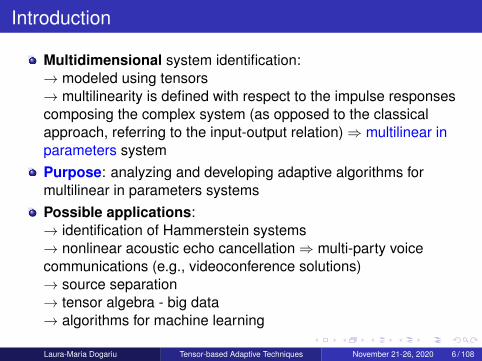
Multidimensional system identification:→ modeled using tensors→ multilinearity is defined with respect to the impulse responsescomposing the complex system (as opposed to the classicalapproach, referring to the input-output relation)⇒ multilinear inparameters system
Purpose: analyzing and developing adaptive algorithms formultilinear in parameters systemsPossible applications:→ identification of Hammerstein systems→ nonlinear acoustic echo cancellation⇒ multi-party voicecommunications (e.g., videoconference solutions)→ source separation→ tensor algebra - big data→ algorithms for machine learning
Laura-Maria Dogariu Tensor-based Adaptive Techniques November 21-26, 2020 6 / 108

Introduction
Multidimensional system identification:→ modeled using tensors→ multilinearity is defined with respect to the impulse responsescomposing the complex system (as opposed to the classicalapproach, referring to the input-output relation)⇒ multilinear inparameters systemPurpose: analyzing and developing adaptive algorithms formultilinear in parameters systems
Possible applications:→ identification of Hammerstein systems→ nonlinear acoustic echo cancellation⇒ multi-party voicecommunications (e.g., videoconference solutions)→ source separation→ tensor algebra - big data→ algorithms for machine learning
Laura-Maria Dogariu Tensor-based Adaptive Techniques November 21-26, 2020 6 / 108
Introduction
Multidimensional system identification:→ modeled using tensors→ multilinearity is defined with respect to the impulse responsescomposing the complex system (as opposed to the classicalapproach, referring to the input-output relation)⇒ multilinear inparameters systemPurpose: analyzing and developing adaptive algorithms formultilinear in parameters systemsPossible applications:→ identification of Hammerstein systems→ nonlinear acoustic echo cancellation⇒ multi-party voicecommunications (e.g., videoconference solutions)→ source separation→ tensor algebra - big data→ algorithms for machine learning
Laura-Maria Dogariu Tensor-based Adaptive Techniques November 21-26, 2020 6 / 108

Outline
1 Introduction
2 Bilinear Forms
3 Trilinear Forms
4 Multilinear Forms
5 Nearest Kronecker Product Decomposition and Low-RankApproximation
6 An Adaptive Solution for Nonlinear System Identification
7 Conclusions
8 Summary of ContributionsLaura-Maria Dogariu Tensor-based Adaptive Techniques November 21-26, 2020 7 / 108
System Model for Bilinear Forms
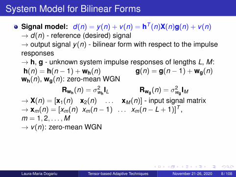
Signal model: d(n) = y(n) + v(n) = hT (n)X(n)g(n) + v(n)→ d(n) - reference (desired) signal→ output signal y(n) - bilinear form with respect to the impulseresponses→ h, g - unknown system impulse responses of lengths L, M:h(n) = h(n − 1) + wh(n) g(n) = g(n − 1) + wg(n)
wh(n), wg(n): zero-mean WGNRwh(n) = σ2
whIL Rwg(n) = σ2
wg IM→ X(n) = [x1(n) x2(n) . . . xM(n)] - input signal matrix→ xm(n) = [xm(n) xm(n − 1) . . . xm(n − L + 1)]T ,m = 1,2, . . . ,M→ v(n): zero-mean WGN
Equivalent model: d(n) = fT (n)x(n) + v(n)→ f(n) = g(n)⊗ h(n)− Kronecker product of length ML→ x(n) = vec[X(n)] = [xT
1 (n) xT2 (n) . . . xT
M(n)]T
Laura-Maria Dogariu Tensor-based Adaptive Techniques November 21-26, 2020 8 / 108

System Model for Bilinear Forms
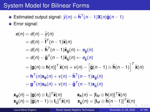
Estimated output signal: y(n) = hT (n − 1)X(n)g(n − 1)
Error signal:
e(n) = d(n)− y(n)
= d(n)− fT (n − 1)x(n)
= d(n)− hT (n − 1)xg(n)← eg(n)
= d(n)− gT (n − 1)xh(n)← eh(n)
= [g(n)⊗ h(n)]T x(n) + v(n)−[g(n − 1)⊗ h(n − 1)
]Tx(n)
= hT (n)xg(n) + v(n)− hT (n − 1)xg(n)
= gT (n)xh(n) + v(n)− gT (n − 1)xh(n)
xg(n) = [g(n)⊗ IL]T x(n) xh(n) = [IM ⊗ h(n)]T x(n)
xg(n) = [g(n − 1)⊗ IL]T x(n) xh(n) = [IM ⊗ h(n − 1)]T x(n)
Laura-Maria Dogariu Tensor-based Adaptive Techniques November 21-26, 2020 9 / 108
System Model for Bilinear Forms
Estimated output signal: y(n) = hT (n − 1)X(n)g(n − 1)
Error signal:
e(n) = d(n)− y(n)
= d(n)− fT (n − 1)x(n)
= d(n)− hT (n − 1)xg(n)← eg(n)
= d(n)− gT (n − 1)xh(n)← eh(n)
= [g(n)⊗ h(n)]T x(n) + v(n)−[g(n − 1)⊗ h(n − 1)
]Tx(n)
= hT (n)xg(n) + v(n)− hT (n − 1)xg(n)
= gT (n)xh(n) + v(n)− gT (n − 1)xh(n)
xg(n) = [g(n)⊗ IL]T x(n) xh(n) = [IM ⊗ h(n)]T x(n)
xg(n) = [g(n − 1)⊗ IL]T x(n) xh(n) = [IM ⊗ h(n − 1)]T x(n)
Laura-Maria Dogariu Tensor-based Adaptive Techniques November 21-26, 2020 9 / 108
Optimized LMS Algorithm for Bilinear Forms
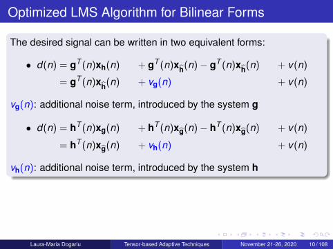
The desired signal can be written in two equivalent forms:
• d(n) = gT (n)xh(n) + gT (n)xh(n)− gT (n)xh(n) + v(n)
= gT (n)xh(n) + vg(n) + v(n)
vg(n): additional noise term, introduced by the system g
• d(n) = hT (n)xg(n) + hT (n)xg(n)− hT (n)xg(n) + v(n)
= hT (n)xg(n) + vh(n) + v(n)
vh(n): additional noise term, introduced by the system h
In the context of LMS:
g(n) = g(n − 1) + µgxh(n)e(n) h(n) = h(n − 1) + µhxg(n)e(n)
Laura-Maria Dogariu Tensor-based Adaptive Techniques November 21-26, 2020 10 / 108

Optimized LMS Algorithm for Bilinear Forms
The desired signal can be written in two equivalent forms:
• d(n) = gT (n)xh(n) + gT (n)xh(n)− gT (n)xh(n) + v(n)
= gT (n)xh(n) + vg(n) + v(n)
vg(n): additional noise term, introduced by the system g
• d(n) = hT (n)xg(n) + hT (n)xg(n)− hT (n)xg(n) + v(n)
= hT (n)xg(n) + vh(n) + v(n)
vh(n): additional noise term, introduced by the system h
In the context of LMS:
g(n) = g(n − 1) + µgxh(n)e(n) h(n) = h(n − 1) + µhxg(n)e(n)
Laura-Maria Dogariu Tensor-based Adaptive Techniques November 21-26, 2020 10 / 108
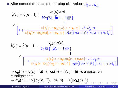
After computations⇒ optimal step-size values µg,o, µh,o:
g(n) = g(n − 1) +xh(n)e(n)
Mσ2xE{||h(n − 1)||2
}× 1[
1 +E{
cTg (n−1)xh(n)c
Th (n−1)xg(n)
}+σ2
v+σ2vg (n)
E{
cTg (n−1)xh(n)c
Th (n−1)xg(n)
}+σ2
xE{||h(n−1)||2
}[mg(n−1)+Mσ2
wg
]]
h(n) = h(n − 1) +xg(n)e(n)
Lσ2xE{||g(n − 1)||2
}× 1[
1 +E{
cTh (n−1)xg(n)c
Tg (n−1)xh(n)
}+σ2
v+σ2vh(n)
E{
cTh (n−1)xg(n)c
Tg (n−1)xh(n)
}+σ2
xE{||g(n−1)||2
}[mh(n−1)+Lσ2
wh
]]→ cg(n) = g(n)− g(n), ch(n) = h(n)− h(n): a posteriorimisalignments→ mg(n) = E
{||cg(n)||2
}, mh(n) = E
{||ch(n)||2
}Laura-Maria Dogariu Tensor-based Adaptive Techniques November 21-26, 2020 11 / 108

Scaling Ambiguity
f(n) = g(n)⊗ h(n) = [ηg(n)]⊗[
1ηh(n)
]η ∈ R∗ - scaling factor
[1ηh(n)
]TX(n) [ηg(n)] = hT (n)X(n)g(n)
⇒h(n)→ 1
ηh(n)
g(n)→ ηg(n)
f(n)→ f(n)
Normalized projection misalignment (NPM):[Morgan et al., IEEE Signal Processing Letters, July 1998]
NPM[h(n), h(n)] = 1−[
hT (n)h(n)||h(n)||||h(n)||
]2
NPM[g(n), g(n)] = 1−[
gT (n)g(n)||g(n)||||g(n)||
]2
Normalized misalignment (NM):
NM[f(n), f(n)] = ‖f(n)− f(n)‖2/‖f(n)‖2
Laura-Maria Dogariu Tensor-based Adaptive Techniques November 21-26, 2020 12 / 108

Scaling Ambiguity
f(n) = g(n)⊗ h(n) = [ηg(n)]⊗[
1ηh(n)
]η ∈ R∗ - scaling factor
[1ηh(n)
]TX(n) [ηg(n)] = hT (n)X(n)g(n)⇒
h(n)→ 1ηh(n)
g(n)→ ηg(n)
f(n)→ f(n)
Normalized projection misalignment (NPM):[Morgan et al., IEEE Signal Processing Letters, July 1998]
NPM[h(n), h(n)] = 1−[
hT (n)h(n)||h(n)||||h(n)||
]2
NPM[g(n), g(n)] = 1−[
gT (n)g(n)||g(n)||||g(n)||
]2
Normalized misalignment (NM):
NM[f(n), f(n)] = ‖f(n)− f(n)‖2/‖f(n)‖2
Laura-Maria Dogariu Tensor-based Adaptive Techniques November 21-26, 2020 12 / 108

Simulation SetupInput signals xm(n),m = 1,2, . . . ,M - independent WGN,respectively AR(1) generated by filtering a white Gaussian noisethrough a first-order system 1/
(1− 0.8z−1)
h, g - Gaussian, randomly generated, of lengths L = 64, M = 8v(n) - independent WGN of variance σ2
v = 0.01
Assumptions: → E{
cTg (n − 1)xh(n)cT
h (n − 1)xg(n)} not .
= pg(n) = 0
→ E{
cTh (n − 1)xg(n)cT
g (n − 1)xh(n)} not .
= ph(n) = 0Performance measure - NM for the global filter
Compared algorithmsOLMS-BF and NLMS-BF [C. Paleologu et al., ”Adaptive filtering for the
identification of bilinear forms,” Digital Signal Process., Apr. 2018]
OLMS-BF and regular JO-NLMS [S. Ciochina et al., ”An optimized NLMS
algorithm for system identification,” Signal Process., 2016]
Laura-Maria Dogariu Tensor-based Adaptive Techniques November 21-26, 2020 13 / 108
0 2 4 6 8 10 12 14 16
Iterations ×104
-50
-40
-30
-20
-10
0
10
No
rma
lize
d m
isa
lig
nm
en
t (d
B)
OLMS-BF
NLMS-BF, αh= α
g= 0.5
NLMS-BF, αh= α
g= 0.01
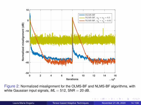
Figure 2: Normalized misalignment for the OLMS-BF and NLMS-BF algorithms, withwhite Gaussian input signals, ML = 512, SNR = 20 dB.
Laura-Maria Dogariu Tensor-based Adaptive Techniques November 21-26, 2020 14 / 108

0 0.5 1 1.5 2 2.5 3 3.5 4 4.5 5
Iterations ×105
-50
-40
-30
-20
-10
0
10
No
rma
lize
d m
isa
lig
nm
en
t (d
B)
OLMS-BF
NLMS-BF, αh= α
g= 0.5
NLMS-BF, αh= α
g= 0.01
Figure 3: Normalized misalignment for the OLMS-BF and NLMS-BF algorithms, withAR(1) input signals, ML = 512, SNR = 20 dB.
Laura-Maria Dogariu Tensor-based Adaptive Techniques November 21-26, 2020 15 / 108
0 2 4 6 8 10 12
Iterations ×104
-40
-35
-30
-25
-20
-15
-10
-5
0
5
10
No
rma
lize
d m
isa
lig
nm
en
t (d
B)
OLMS-BF
JO-NLMS
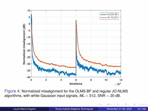
Figure 4: Normalized misalignment for the OLMS-BF and regular JO-NLMSalgorithms, with white Gaussian input signals, ML = 512, SNR = 20 dB.
Laura-Maria Dogariu Tensor-based Adaptive Techniques November 21-26, 2020 16 / 108

0 2 4 6 8 10 12
Iterations ×104
-40
-35
-30
-25
-20
-15
-10
-5
0
5
10
No
rma
lize
d m
isa
lig
nm
en
t (d
B)
OLMS-BF
JO-NLMS
Figure 5: Normalized misalignment for the OLMS-BF and regular JO-NLMSalgorithms, with AR(1) input signals, ML = 512, SNR = 20 dB.
Laura-Maria Dogariu Tensor-based Adaptive Techniques November 21-26, 2020 17 / 108

Kalman Filter for Bilinear Forms (KF-BF)
A posteriori misalignments:
ch(n) =1η
h(n)− h(n) cg(n) = ηg(n)− g(n)
→ with correlation matrices:
Rch(n) = E[ch(n)cTh (n)] Rcg(n) = E[cg(n)cT
g (n)]
A priori misalignments:
cha(n) =1η
h(n)− h(n − 1)
= ch(n − 1) +1η
wh(n)
cga(n) = ηg(n)− g(n − 1)
= cg(n − 1) + ηwg(n)
→ with correlation matrices:
Rcha(n) = E
[cha(n)cT
ha(n)]
Rcga(n) = E
[cga(n)cT
ga(n)]
Rcha(n) = Rch(n − 1) + σ2
whIL Rcga
(n) = Rcg(n − 1) + σ2wg IM
Laura-Maria Dogariu Tensor-based Adaptive Techniques November 21-26, 2020 18 / 108
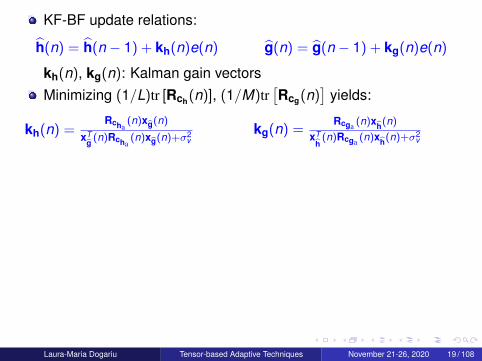
KF-BF update relations:
h(n) = h(n − 1) + kh(n)e(n) g(n) = g(n − 1) + kg(n)e(n)
kh(n), kg(n): Kalman gain vectorsMinimizing (1/L)tr [Rch(n)], (1/M)tr
[Rcg(n)
]yields:
kh(n) =Rcha
(n)xg(n)
xTg (n)Rcha
(n)xg(n)+σ2v
kg(n) =Rcga (n)xh(n)
xTh(n)Rcga (n)xh(n)+σ
2v
Simplifying assumptions:after convergence was reached:
Rcha(n) ≈ σ2
cha(n)IL Rcga
(n) ≈ σ2cga
(n)IMmisalignments of the individual coefficients: uncorrelated⇒ we can approximate:
IL − kh(n)xTg (n) ≈
[1− 1
LkTh (n)xg(n)
]IL
IM − kg(n)xTh
(n) ≈[1− 1
M kTg (n)xh(n)
]IM
⇒ Simplified Kalman Filter for bilinear forms (SKF - BF)
Laura-Maria Dogariu Tensor-based Adaptive Techniques November 21-26, 2020 19 / 108

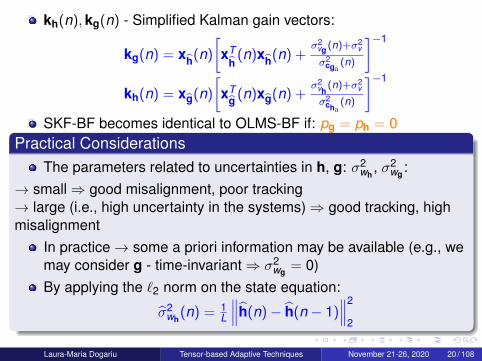
kh(n),kg(n) - Simplified Kalman gain vectors:
kg(n) = xh(n)
[xT
h(n)xh(n) +
σ2vg (n)+σ
2v
σ2cga
(n)
]−1
kh(n) = xg(n)
[xT
g (n)xg(n) +σ2
vh(n)+σ2
v
σ2cha
(n)
]−1
SKF-BF becomes identical to OLMS-BF if: pg = ph = 0Practical Considerations
The parameters related to uncertainties in h, g: σ2wh
, σ2wg :
→ small⇒ good misalignment, poor tracking→ large (i.e., high uncertainty in the systems)⇒ good tracking, highmisalignment
In practice→ some a priori information may be available (e.g., wemay consider g - time-invariant⇒ σ2
wg = 0)By applying the `2 norm on the state equation:
σ2wh
(n) = 1L
∥∥∥h(n)− h(n − 1)∥∥∥2
2
Laura-Maria Dogariu Tensor-based Adaptive Techniques November 21-26, 2020 20 / 108

kh(n),kg(n) - Simplified Kalman gain vectors:
kg(n) = xh(n)
[xT
h(n)xh(n) +
σ2vg (n)+σ
2v
σ2cga
(n)
]−1
kh(n) = xg(n)
[xT
g (n)xg(n) +σ2
vh(n)+σ2
v
σ2cha
(n)
]−1
SKF-BF becomes identical to OLMS-BF if: pg = ph = 0
Practical ConsiderationsThe parameters related to uncertainties in h, g: σ2
wh, σ2
wg :→ small⇒ good misalignment, poor tracking→ large (i.e., high uncertainty in the systems)⇒ good tracking, highmisalignment
In practice→ some a priori information may be available (e.g., wemay consider g - time-invariant⇒ σ2
wg = 0)By applying the `2 norm on the state equation:
σ2wh
(n) = 1L
∥∥∥h(n)− h(n − 1)∥∥∥2
2
Laura-Maria Dogariu Tensor-based Adaptive Techniques November 21-26, 2020 20 / 108
kh(n),kg(n) - Simplified Kalman gain vectors:
kg(n) = xh(n)
[xT
h(n)xh(n) +
σ2vg (n)+σ
2v
σ2cga
(n)
]−1
kh(n) = xg(n)
[xT
g (n)xg(n) +σ2
vh(n)+σ2
v
σ2cha
(n)
]−1
SKF-BF becomes identical to OLMS-BF if: pg = ph = 0Practical Considerations
The parameters related to uncertainties in h, g: σ2wh
, σ2wg :
→ small⇒ good misalignment, poor tracking→ large (i.e., high uncertainty in the systems)⇒ good tracking, highmisalignment
In practice→ some a priori information may be available (e.g., wemay consider g - time-invariant⇒ σ2
wg = 0)By applying the `2 norm on the state equation:
σ2wh
(n) = 1L
∥∥∥h(n)− h(n − 1)∥∥∥2
2
Laura-Maria Dogariu Tensor-based Adaptive Techniques November 21-26, 2020 20 / 108

0 1 2 3 4 5 6 7 8 9 10
Iterations ×104
-70
-60
-50
-40
-30
-20
-10
0
10
No
rma
lize
d m
isa
lig
nm
en
t (d
B)
KF-BF, WGN inputs
Regular KF, WGN inputs
KF-BF, AR(1) inputs
Regular KF, AR(1) inputs
Figure 6: Normalized misalignment of the KF-BF and regular KF for different types ofinput signals. ML = 512, σ2
v = 0.01, σ2wh = σ2
wg = σ2w = 10−9, and ε = 10−5.
Laura-Maria Dogariu Tensor-based Adaptive Techniques November 21-26, 2020 21 / 108
0 0.5 1 1.5 2 2.5 3
Iterations ×105
-70
-60
-50
-40
-30
-20
-10
0
10
No
rma
lize
d m
isa
lig
nm
en
t (d
B)
SKF-BF, WGN inputs
Regular SKF, WGN inputs
SKF-BF, AR(1) inputs
Regular SKF, AR(1) inputs
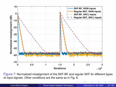
Figure 7: Normalized misalignment of the SKF-BF and regular SKF for different typesof input signals. Other conditions are the same as in Fig. 6.
Laura-Maria Dogariu Tensor-based Adaptive Techniques November 21-26, 2020 22 / 108

0 2 4 6 8 10 12 14
Iterations ×104
-80
-70
-60
-50
-40
-30
-20
-10
0
10
No
rmalized
mis
alig
nm
en
t (d
B)
SKF-BF, WGN inputs
Regular SKF, WGN inputs
SKF-BF, AR(1) inputs
Regular SKF, AR(1) inputs
Figure 8: Normalized misalignment of the SKF-BF and regular SKF for different typesof input signals, using the recursive estimates σ2
wh(n) and σ2w (n), respectively.
ML = 512, σ2v = 0.01, σ2
wg = 0, and ε = 10−5.
Laura-Maria Dogariu Tensor-based Adaptive Techniques November 21-26, 2020 23 / 108

Improved Proportionate APA for the Identification ofSparse Bilinear forms
Motivation:Echo cancellation - a particular type of system identificationproblem - estimate a model (echo path) using the available andobserved data (usually input and output of the system)The echo paths are sparse in nature: only a few impulseresponse components have a significant magnitude, while the restare zero or smallProportionate algorithms: adjust the adaptation step-size inproportion to the magnitude of the estimated filter coefficientAffine Projection Algorithm (APA): frequently used in echocancellation, due to its fast convergence
Target: A proportionate APA for the identification of sparse bilinearforms
Laura-Maria Dogariu Tensor-based Adaptive Techniques November 21-26, 2020 24 / 108
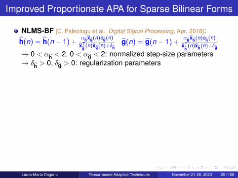
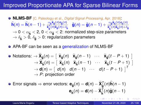
Improved Proportionate APA for Sparse Bilinear Forms
NLMS-BF [C. Paleologu et al., Digital Signal Processing, Apr. 2018]:h(n) = h(n − 1) +
αhxg(n)eg(n)xT
g (n)xg(n)+δhg(n) = g(n − 1) +
αgxh(n)eh(n)xT
h(n)xh(n)+δg
→ 0 < αh < 2, 0 < αg < 2: normalized step-size parameters→ δh > 0, δg > 0: regularization parameters
APA-BF can be seen as a generalization of NLMS-BF
Notations: → Xg(n) =[
xg(n) xg(n − 1) · · · xg(t − P + 1)]
→ Xh(n) =[
xh(n) xh(n − 1) · · · xh(t − P + 1)]
→ d(n) =[
d(n) d(n − 1) · · · d(t − P + 1)]T
→ P: projection order
Error signals⇒ error vectors: eg(n) = d(n)− XTg (n)h(n − 1)
eh(n) = d(n)− XTh
(n)g(n − 1)
Laura-Maria Dogariu Tensor-based Adaptive Techniques November 21-26, 2020 25 / 108

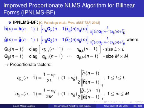
Improved Proportionate NLMS Algorithm for BilinearForms (IPNLMS-BF)
IPNLMS-BF: [C. Paleologu et al., Proc. IEEE TSP, 2018]
h(n) = h(n − 1) +[αhQh(n − 1)xg(n)eg(n)
]1
xTg (n)Qh(n−1)xg(n)+δh
g(n) = g(n − 1) +[αgQg(n − 1)xh(n)eh(n)
]1
xTh(n)Qg(n−1)xh(n)+δg
where
Qh(n − 1) = diag[
qh,1(n − 1) · · · qh,L(n − 1)]
- size L× L
Qg(n − 1) = diag[
qg,1(n − 1) · · · qg,M(n − 1)]
- size M ×M
→ Proportionate factors:
qh,l(n − 1) =1− κh
2L+ (1 + κh)
∣∣∣hl(n − 1)∣∣∣
2∥∥∥h(n − 1)
∥∥∥1
, 1 ≤ l ≤ L
qg,m(n − 1) =1− κg
2M+ (1 + κg)
∣∣gm(n − 1)∣∣
2∥∥g(n − 1)
∥∥1
, 1 ≤ m ≤ M
Laura-Maria Dogariu Tensor-based Adaptive Techniques November 21-26, 2020 26 / 108

Improved Proportionate APA for Bilinear Forms
IPAPA-BF:h(n) = h(n − 1) + αhQh(n − 1)Xg(n)
[XT
g (n)Qh(n − 1)Xg(n) + δhIP]−1
eg(n)
g(n) = g(n − 1) + αgQg(n − 1)Xh(n)[XT
h(n)Qg(n − 1)Xh(n) + δgIP
]−1eh(n)
→ Qh,Qg: matrices containing proportionality factors→ if P = 1⇒ IPNLMS-BF→ if Qh(n − 1) = IL, Qg(n − 1) = IM ⇒ APA-BF
Experiments - system identification:h, of length L = 512: the first impulse response from G168Recommendation, padded with zeros [Digital Network Echo Cancellers,ITU-T Recommendations G.168, 2002]
g, of length M = 4: computed as gm = 0.5m, m = 1, . . . ,M
Laura-Maria Dogariu Tensor-based Adaptive Techniques November 21-26, 2020 27 / 108

0 1 2 3 4 5
Iterations ×104
-35
-30
-25
-20
-15
-10
-5
0
NM
(dB)
NLMS− BFAPA− BF, P = 2APA− BF, P = 4
Figure 9: Performance of the NLMS-BF and APA-BF in terms of NM. The inputsignals are AR(1) processes and ML = 2048.
Laura-Maria Dogariu Tensor-based Adaptive Techniques November 21-26, 2020 28 / 108
0 0.5 1 1.5 2
Iterations ×104
-35
-30
-25
-20
-15
-10
-5
0
NM
(dB)
IPNLMS− BFIPAPA− BF, P = 2IPAPA− BF, P = 4
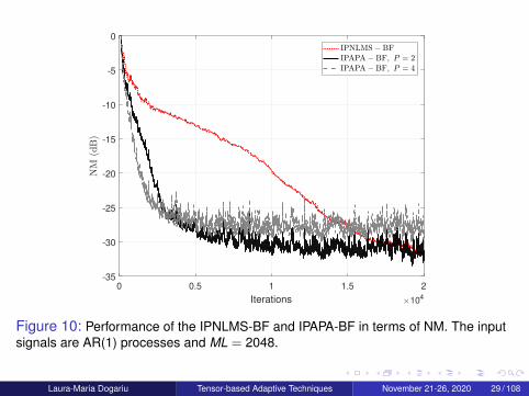
Figure 10: Performance of the IPNLMS-BF and IPAPA-BF in terms of NM. The inputsignals are AR(1) processes and ML = 2048.
Laura-Maria Dogariu Tensor-based Adaptive Techniques November 21-26, 2020 29 / 108

0 0.5 1 1.5 2 2.5 3
Iterations ×104
-35
-30
-25
-20
-15
-10
-5
0
NM
(dB)
APA, α = 0.2APA− BF, α
h= α
g= 0.1
IPAPA− BF, αh= α
g= 0.1
Figure 11: Performance of the APA, APA-BF, and IPAPA-BF in terms of NM. The inputsignals are white Gaussian noises and ML = 2048.
Laura-Maria Dogariu Tensor-based Adaptive Techniques November 21-26, 2020 30 / 108
0 0.5 1 1.5 2
Iterations ×104
-35
-30
-25
-20
-15
-10
-5
0
NM
(dB)
IPAPA, α = 1IPAPA, α = 0.2
IPAPA− BF, αh= α
g= 0.1
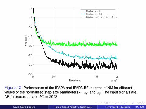
Figure 12: Performance of the IPAPA and IPAPA-BF in terms of NM for differentvalues of the normalized step-size parameters α, αh, and αg. The input signals areAR(1) processes and ML = 2048.
Laura-Maria Dogariu Tensor-based Adaptive Techniques November 21-26, 2020 31 / 108

Outline
1 Introduction
2 Bilinear Forms
3 Trilinear Forms
4 Multilinear Forms
5 Nearest Kronecker Product Decomposition and Low-RankApproximation
6 An Adaptive Solution for Nonlinear System Identification
7 Conclusions
8 Summary of ContributionsLaura-Maria Dogariu Tensor-based Adaptive Techniques November 21-26, 2020 32 / 108

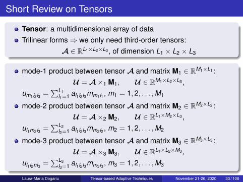
Short Review on Tensors
Tensor: a multidimensional array of dataTrilinear forms⇒ we only need third-order tensors:
A ∈ RL1×L2×L3 , of dimension L1 × L2 × L3
mode-1 product between tensor A and matrix M1 ∈ RM1×L1 :U = A×1 M1, U ∈ RM1×L2×L3 ,
um1l2l3 =∑L1
l1=1 al1l2l3mm1l1 , m1 = 1,2, . . . ,M1
mode-2 product between tensor A and matrix M2 ∈ RM2×L2 :U = A×2 M2, U ∈ RL1×M2×L3 ,
ul1m2l3 =∑L2
l2=1 al1l2l3mm2l2 , m2 = 1,2, . . . ,M2
mode-3 product between tensor A and matrix M3 ∈ RM3×L3 :U = A×3 M3, U ∈ RL1×L2×M3 ,
ul1l2m3 =∑L3
l3=1 al1l2l3mm3l3 , m3 = 1,2, . . . ,M3
Laura-Maria Dogariu Tensor-based Adaptive Techniques November 21-26, 2020 33 / 108

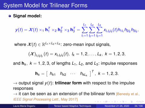
System Model for Trilinear Forms
Signal model:
y(t) = X (t)×1 hT1 ×2 hT
2 ×3 hT3 =
L1∑l1=1
L2∑l2=1
L3∑l3=1
xl1l2l3(t)h1l1h2l2h3l3 ,
where X (t) ∈ RL1×L2×L3 : zero-mean input signals,
(X )l1l2l3 (t) = xl1l2l3(t), lk = 1,2, . . . ,Lk , k = 1,2,3,
and hk , k = 1,2,3, of lengths L1, L2, and L3: impulse responses
hk =[
hk1 hk2 · · · hkLk
]T, k = 1,2,3.
→ output signal y(t): trilinear form with respect to the impulseresponses→ it can be seen as an extension of the bilinear form [Benesty et al.,IEEE Signal Processing Lett., May 2017]
Laura-Maria Dogariu Tensor-based Adaptive Techniques November 21-26, 2020 34 / 108
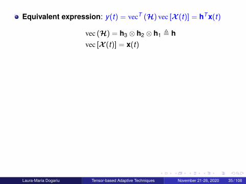
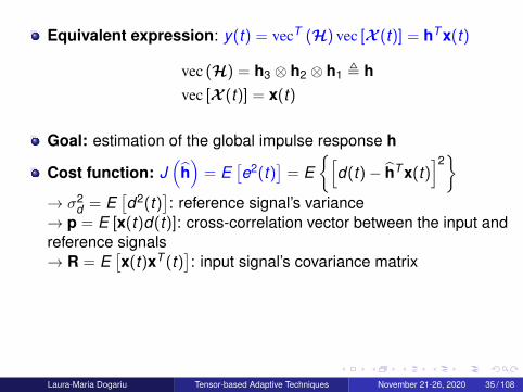
Equivalent expression: y(t) = vecT (H) vec [X (t)] = hT x(t)
vec (H) = h3 ⊗ h2 ⊗ h1 , hvec [X (t)] = x(t)
Goal: estimation of the global impulse response h
Cost function: J(
h)
= E[e2(t)
]= E
{[d(t)− hT x(t)
]2}
→ σ2d = E
[d2(t)
]: reference signal’s variance
→ p = E [x(t)d(t)]: cross-correlation vector between the input andreference signals→ R = E
[x(t)xT (t)
]: input signal’s covariance matrix
After computations: J(
h)
= σ2d − 2hT p + hT Rh
Minimize J(
h)⇒ conventional Wiener filter: hW = R−1p
Laura-Maria Dogariu Tensor-based Adaptive Techniques November 21-26, 2020 35 / 108
Iterative Wiener Filter for Trilinear Forms
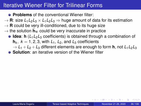
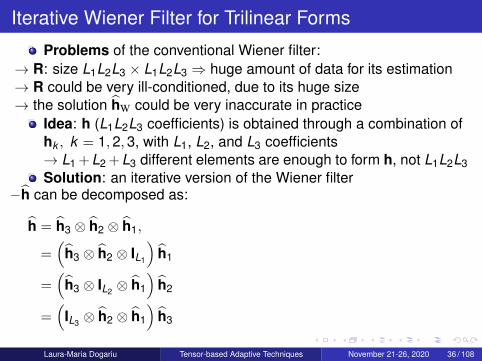
Problems of the conventional Wiener filter:→ R: size L1L2L3 × L1L2L3 ⇒ huge amount of data for its estimation→ R could be very ill-conditioned, due to its huge size→ the solution hW could be very inaccurate in practice
Idea: h (L1L2L3 coefficients) is obtained through a combination ofhk , k = 1,2,3, with L1, L2, and L3 coefficients→ L1 + L2 + L3 different elements are enough to form h, not L1L2L3Solution: an iterative version of the Wiener filter
−h can be decomposed as:
h = h3 ⊗ h2 ⊗ h1,
=(
h3 ⊗ h2 ⊗ IL1
)h1
=(
h3 ⊗ IL2 ⊗ h1
)h2
=(
IL3 ⊗ h2 ⊗ h1
)h3
− in a corresponding manner, J(
h)
canbe written as:
Jh2,h3
(h1
)= σ2
d − 2hT1 p1 + hT
1 R1h1
Jh1,h3
(h2
)= σ2
d − 2hT2 p2 + hT
2 R2h2
Jh1,h2
(h3
)= σ2
d − 2hT3 p3 + hT
3 R3h3
Laura-Maria Dogariu Tensor-based Adaptive Techniques November 21-26, 2020 36 / 108
Iterative Wiener Filter for Trilinear Forms
Problems of the conventional Wiener filter:→ R: size L1L2L3 × L1L2L3 ⇒ huge amount of data for its estimation→ R could be very ill-conditioned, due to its huge size→ the solution hW could be very inaccurate in practice
Idea: h (L1L2L3 coefficients) is obtained through a combination ofhk , k = 1,2,3, with L1, L2, and L3 coefficients→ L1 + L2 + L3 different elements are enough to form h, not L1L2L3Solution: an iterative version of the Wiener filter
−h can be decomposed as:
h = h3 ⊗ h2 ⊗ h1,
=(
h3 ⊗ h2 ⊗ IL1
)h1
=(
h3 ⊗ IL2 ⊗ h1
)h2
=(
IL3 ⊗ h2 ⊗ h1
)h3
− in a corresponding manner, J(
h)
canbe written as:
Jh2,h3
(h1
)= σ2
d − 2hT1 p1 + hT
1 R1h1
Jh1,h3
(h2
)= σ2
d − 2hT2 p2 + hT
2 R2h2
Jh1,h2
(h3
)= σ2
d − 2hT3 p3 + hT
3 R3h3
Laura-Maria Dogariu Tensor-based Adaptive Techniques November 21-26, 2020 36 / 108

Iterative Wiener Filter for Trilinear Forms
wherep1 =
(h3 ⊗ h2 ⊗ IL1
)Tp,
R1 =(
h3 ⊗ h2 ⊗ IL1
)TR(
h3 ⊗ h2 ⊗ IL1
),
p2 =(
h3 ⊗ IL2 ⊗ h1
)Tp,
R2 =(
h3 ⊗ IL2 ⊗ h1
)TR(
h3 ⊗ IL2 ⊗ h1
),
p3 =(
IL3 ⊗ h2 ⊗ h1
)Tp,
R3 =(
IL3 ⊗ h2 ⊗ h1
)TR(
IL3 ⊗ h2 ⊗ h1
).
Initialize:
h(0)2 = (1/L2)
[1 1 · · · 1
]Th(0)
3 = (1/L3)[
1 1 · · · 1]T
Laura-Maria Dogariu Tensor-based Adaptive Techniques November 21-26, 2020 37 / 108
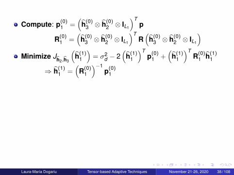
Compute: p(0)1 =
(h(0)
3 ⊗ h(0)2 ⊗ IL1
)Tp
R(0)1 =
(h(0)
3 ⊗ h(0)2 ⊗ IL1
)TR(
h(0)3 ⊗ h(0)
2 ⊗ IL1
)Minimize Jh2,h3
(h(1)
1
)= σ2
d − 2(
h(1)1
)Tp(0)
1 +(
h(1)1
)TR(0)
1 h(1)1
⇒ h(1)1 =
(R(0)
1
)−1p(0)
1
Compute: p(1)2 =
(h(0)
3 ⊗ IL2 ⊗ h(1)1
)Tp
R(1)2 =
(h(0)
3 ⊗ IL2 ⊗ h(1)1
)TR(
h(0)3 ⊗ IL2 ⊗ h(1)
1
)Minimize Jh1,h3
(h(1)
2
)= σ2
d − 2(
h(1)2
)Tp(1)
2 +(
h(1)2
)TR(1)
2 h(1)2
⇒ h(1)2 =
(R(1)
2
)−1p(1)
2
Laura-Maria Dogariu Tensor-based Adaptive Techniques November 21-26, 2020 38 / 108
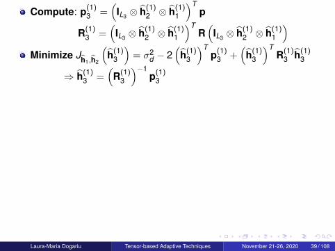
Compute: p(1)3 =
(IL3 ⊗ h(1)
2 ⊗ h(1)1
)Tp
R(1)3 =
(IL3 ⊗ h(1)
2 ⊗ h(1)1
)TR(
IL3 ⊗ h(1)2 ⊗ h(1)
1
)Minimize Jh1,h2
(h(1)
3
)= σ2
d − 2(
h(1)3
)Tp(1)
3 +(
h(1)3
)TR(1)
3 h(1)3
⇒ h(1)3 =
(R(1)
3
)−1p(1)
3
At iteration n:
h(n)1 =
(R(n−1)
1
)−1p(n−1)
1 , p(n)2 =
(h(n−1)
3 ⊗ IL2 ⊗ h(n)1
)Tp,
R(n)2 =
(h(n−1)
3 ⊗ IL2 ⊗ h(n)1
)TR(
h(n−1)3 ⊗ IL2 ⊗ h(n)
1
),
h(n)2 =
(R(n)
2
)−1p(n)
2 , p(n)3 =
(IL3 ⊗ h(n)
2 ⊗ h(n)1
)Tp,
R(n)3 =
(IL3 ⊗ h(n)
2 ⊗ h(n)1
)TR(
IL3 ⊗ h(n)2 ⊗ h(n)
1
),
h(n)3 =
(R(n)
3
)−1p(n)
3 .
Finally: h(n) = h(n)3 ⊗ h(n)
2 ⊗ h(n)1
Laura-Maria Dogariu Tensor-based Adaptive Techniques November 21-26, 2020 39 / 108

Samples
20 40 60
Am
plit
ude
-0.1
0
0.1
0.2
(a)
Samples
2 4 6 8
Am
plit
ude
-1
0
1
2(b)
Samples
1 2 3 4
Am
plit
ude
0
0.5
1(c)
Samples
200 400 600 800 1000 1200 1400 1600 1800 2000
Am
plit
ude
-0.2
0
0.2
0.4
(d)
Figure 13: Impulse responses used in simulations: (a) h1 of length L1 = 64 [Digital
Network Echo Cancellers, ITU-T Recommendations G.168, 2002.], (b) h2 of length L2 = 8 (randomlygenerated), (c) h3 of length L3 = 4 (evaluated as h3l3 = 0.5l3−1, l3 = 1, . . . , L3), (d)global impulse response h = h3 ⊗ h2 ⊗ h1 of length L = L1L2L3 = 2048.
Laura-Maria Dogariu Tensor-based Adaptive Techniques November 21-26, 2020 40 / 108
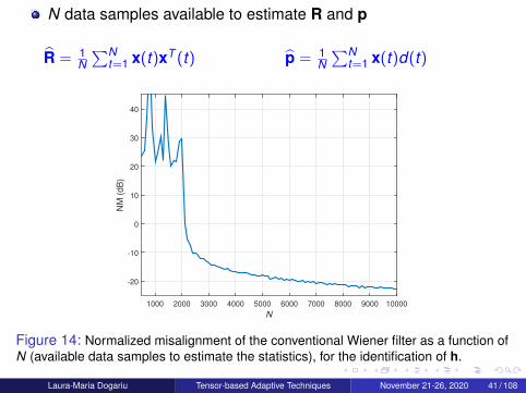
N data samples available to estimate R and p
R = 1N∑N
t=1 x(t)xT (t) p = 1N∑N
t=1 x(t)d(t)
N
1000 2000 3000 4000 5000 6000 7000 8000 9000 10000
NM
(d
B)
-20
-10
0
10
20
30
40
Figure 14: Normalized misalignment of the conventional Wiener filter as a function ofN (available data samples to estimate the statistics), for the identification of h.
Laura-Maria Dogariu Tensor-based Adaptive Techniques November 21-26, 2020 41 / 108

Iterations
2 4 6 8 10 12 14 16 18 20
NM
(dB
)
-40
-30
-20
-10
0
10
20
30
Conventional Wiener filter, N = 500
Conventional Wiener filter, N = 2500
Conventional Wiener filter, N = 5000Iterative Wiener filter, N = 500
Iterative Wiener filter, N = 2500
Iterative Wiener filter, N = 5000
Figure 15: Normalized misalignment of the conventional and iterative Wiener filters,for different values of N (available data samples to estimate the statistics), for theidentification of h.
Laura-Maria Dogariu Tensor-based Adaptive Techniques November 21-26, 2020 42 / 108

Iterations
2 4 6 8 10 12 14 16 18 20N
PM
(dB
)-50
0(a)
N = 500
N = 2500
N = 5000
Iterations
2 4 6 8 10 12 14 16 18 20
NP
M (
dB
)
-50
0(b)
N = 500
N = 2500
N = 5000
Iterations
2 4 6 8 10 12 14 16 18 20
NP
M (
dB
)
-50
0(c)
N = 500
N = 2500
N = 5000
Figure 16: Normalized projection misalignment of the iterative Wiener filter, fordifferent values of N (available data samples to estimate the statistics), for theidentification of h1,h2,h3
Laura-Maria Dogariu Tensor-based Adaptive Techniques November 21-26, 2020 43 / 108

Iterative Wiener Filter for Trilinear Forms
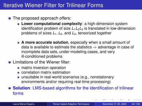
The proposed approach offers:Lower computational complexity: a high-dimension systemidentification problem of size L1L2L3 is translated in low-dimensionproblems of sizes L1,L2, and L3, tensorized together
A more accurate solution, especially when a small amount ofdata is available to estimate the statistics⇒ advantage in case ofincomplete data sets, under-modeling cases, and veryill-conditioned problems
Limitations of the Wiener filter:matrix inversion operationcorrelation matrix estimationunsuitable in real-world scenarios (e.g., nonstationaryenvironments and/or requiring real-time processing)
Solution: LMS-based algorithms for the identification of trilinearforms
Laura-Maria Dogariu Tensor-based Adaptive Techniques November 21-26, 2020 44 / 108
Iterative Wiener Filter for Trilinear Forms
The proposed approach offers:Lower computational complexity: a high-dimension systemidentification problem of size L1L2L3 is translated in low-dimensionproblems of sizes L1,L2, and L3, tensorized together
A more accurate solution, especially when a small amount ofdata is available to estimate the statistics⇒ advantage in case ofincomplete data sets, under-modeling cases, and veryill-conditioned problems
Limitations of the Wiener filter:matrix inversion operationcorrelation matrix estimationunsuitable in real-world scenarios (e.g., nonstationaryenvironments and/or requiring real-time processing)
Solution: LMS-based algorithms for the identification of trilinearforms
Laura-Maria Dogariu Tensor-based Adaptive Techniques November 21-26, 2020 44 / 108

Least-Mean-Square Algorithm for Trilinear Forms(LMS-TF)
A priori error signal can be written (similar to BF) as:
e(t) = d(t)− y(t) = d(t)− h(t − 1)T x(t)
= d(t)− hT1 (t − 1)xh2h3
(t) ← eh2h3(t)
= d(t)− hT2 (t − 1)xh1h3
(t) ← eh1h3(t)
= d(t)− hT3 (t − 1)xh1h2
(t) ← eh1h2(t)
where
xh2h3(t) =
[h3(t − 1)⊗ h2(t − 1)⊗ IL1
]x(t)
xh1h3(t) =
[h3(t − 1)⊗ IL2 ⊗ h1(t − 1)
]x(t)
xh1h2(t) =
[IL3 ⊗ h2(t − 1)⊗ h1(t − 1)
]x(t)
Laura-Maria Dogariu Tensor-based Adaptive Techniques November 21-26, 2020 45 / 108
Least-Mean-Square Algorithm for Trilinear Forms(LMS-TF)
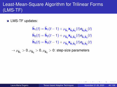
LMS-TF updates:
h1(t) = h1(t − 1) + µh1xh2h3
(t)eh2h3(t)
h2(t) = h2(t − 1) + µh2xh1h3
(t)eh1h3(t)
h3(t) = h3(t − 1) + µh3xh1h2
(t)eh1h2(t)
→ µh1> 0, µh2
> 0, µh3> 0: step-size parameters
LMS-TF uses three short filters, of lengths L1,L2,L3, instead of along filter, of length L1L2L3 ⇒ lower complexityFaster convergence rate expectedFor non-stationary signals: it may be more appropriate to usetime-dependent step-sizes µh1
(t), µh2(t), µh3
(t)
Laura-Maria Dogariu Tensor-based Adaptive Techniques November 21-26, 2020 46 / 108

Least-Mean-Square Algorithm for Trilinear Forms(LMS-TF)
LMS-TF updates:
h1(t) = h1(t − 1) + µh1xh2h3
(t)eh2h3(t)
h2(t) = h2(t − 1) + µh2xh1h3
(t)eh1h3(t)
h3(t) = h3(t − 1) + µh3xh1h2
(t)eh1h2(t)
→ µh1> 0, µh2
> 0, µh3> 0: step-size parameters
LMS-TF uses three short filters, of lengths L1,L2,L3, instead of along filter, of length L1L2L3 ⇒ lower complexityFaster convergence rate expectedFor non-stationary signals: it may be more appropriate to usetime-dependent step-sizes µh1
(t), µh2(t), µh3
(t)
Laura-Maria Dogariu Tensor-based Adaptive Techniques November 21-26, 2020 46 / 108

Normalized LMS Algorithm for Trilinear Forms(NLMS-TF)
A posteriori error signals:
εh2h3(t) = d(t)− hT
1 (t)xh2h3(t)
εh1h3(t) = d(t)− hT
2 (t)xh1h3(t)
εh1h2(t) = d(t)− hT
3 (t)xh1h2(t)
By cancelling the a posteriori error signals⇒ NLMS-TF:
h1(t) = h1(t − 1) +αh1
xh2h3(t)eh2h3
(t)
xTh2h3
(t)xh2h3(t) + δh1
h2(t) = h2(t − 1) +αh2
xh1h3(t)eh1h3
(t)
xTh1h3
(t)xh1h3(t) + δh2
h3(t) = h3(t − 1) +αh3
xh1h2(t)eh1h2
(t)
xTh1h2
(t)xh1h2(t) + δh3
Laura-Maria Dogariu Tensor-based Adaptive Techniques November 21-26, 2020 47 / 108

2 4 6 8 10 12 14 16 18
Iterations 104
-45
-40
-35
-30
-25
-20
-15
-10
-5
0
NM
(d
B)
Figure 17: Normalized misalignment of the LMS-TF algorithm using differentvalues of the step-size parameters.
Laura-Maria Dogariu Tensor-based Adaptive Techniques November 21-26, 2020 48 / 108
0 0.2 0.4 0.6 0.8 1 1.2 1.4 1.6 1.8 2
Iterations 105
-45
-40
-35
-30
-25
-20
-15
-10
-5
0
NM
(d
B)
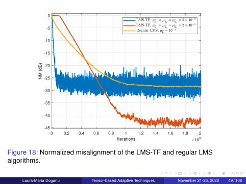
Figure 18: Normalized misalignment of the LMS-TF and regular LMSalgorithms.
Laura-Maria Dogariu Tensor-based Adaptive Techniques November 21-26, 2020 49 / 108

0 2 4 6 8 10 12 14 16 18
Iterations 104
-45
-40
-35
-30
-25
-20
-15
-10
-5
0
NM
(d
B)
Figure 19: Normalized misalignment of the NLMS-TF algorithm usingdifferent values of the step-size parameters.
Laura-Maria Dogariu Tensor-based Adaptive Techniques November 21-26, 2020 50 / 108

0 2 4 6 8 10 12 14 16 18
Iterations 104
-45
-40
-35
-30
-25
-20
-15
-10
-5
0
NM
(d
B)
Figure 20: Normalized misalignment of the NLMS-TF and regular NLMSalgorithms.
Laura-Maria Dogariu Tensor-based Adaptive Techniques November 21-26, 2020 51 / 108
0 0.5 1 1.5 2 2.5 3 3.5 4
Iterations 105
-50
-45
-40
-35
-30
-25
-20
-15
-10
-5
0
NM
(d
B)
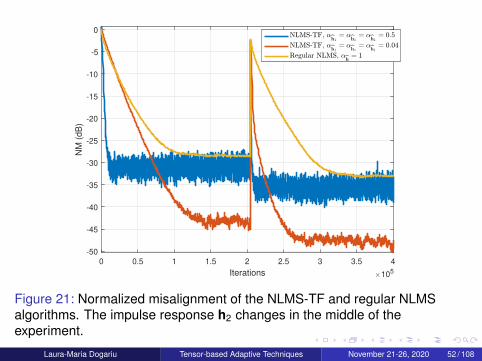
Figure 21: Normalized misalignment of the NLMS-TF and regular NLMSalgorithms. The impulse response h2 changes in the middle of theexperiment.
Laura-Maria Dogariu Tensor-based Adaptive Techniques November 21-26, 2020 52 / 108

Outline
1 Introduction
2 Bilinear Forms
3 Trilinear Forms
4 Multilinear Forms
5 Nearest Kronecker Product Decomposition and Low-RankApproximation
6 An Adaptive Solution for Nonlinear System Identification
7 Conclusions
8 Summary of ContributionsLaura-Maria Dogariu Tensor-based Adaptive Techniques November 21-26, 2020 53 / 108
Iterative Wiener Filter for Multilinear Forms
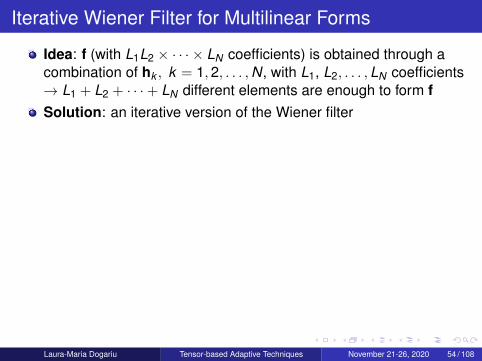
Idea: f (with L1L2 × · · · × LN coefficients) is obtained through acombination of hk , k = 1,2, . . . ,N, with L1, L2, . . . ,LN coefficients→ L1 + L2 + · · ·+ LN different elements are enough to form fSolution: an iterative version of the Wiener filter
→ It can be verified that:
f = hN ⊗ hN−1 ⊗ · · · ⊗ h1
=(hN ⊗ hN−1 ⊗ · · · ⊗ IL1
)h1
=(hN ⊗ hN−1 ⊗ · · · ⊗ h3 ⊗ IL2 ⊗ h1
)h2
...=(hN ⊗ hN−1 ⊗ · · · ⊗ ILi ⊗ hLi−1 ⊗ · · · ⊗ h1
)hi
...=(ILN ⊗ hN−1 ⊗ · · · ⊗ h1
)hN
Laura-Maria Dogariu Tensor-based Adaptive Techniques November 21-26, 2020 54 / 108
Iterative Wiener Filter for Multilinear Forms
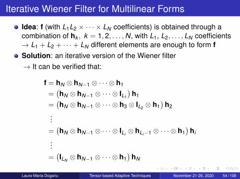
Idea: f (with L1L2 × · · · × LN coefficients) is obtained through acombination of hk , k = 1,2, . . . ,N, with L1, L2, . . . ,LN coefficients→ L1 + L2 + · · ·+ LN different elements are enough to form fSolution: an iterative version of the Wiener filter→ It can be verified that:
f = hN ⊗ hN−1 ⊗ · · · ⊗ h1
=(hN ⊗ hN−1 ⊗ · · · ⊗ IL1
)h1
=(hN ⊗ hN−1 ⊗ · · · ⊗ h3 ⊗ IL2 ⊗ h1
)h2
...=(hN ⊗ hN−1 ⊗ · · · ⊗ ILi ⊗ hLi−1 ⊗ · · · ⊗ h1
)hi
...=(ILN ⊗ hN−1 ⊗ · · · ⊗ h1
)hN
Laura-Maria Dogariu Tensor-based Adaptive Techniques November 21-26, 2020 54 / 108

Iterative Wiener Filter for Multilinear Forms
Consequently, J(
f)
can be written in N equivalent forms
When all coefficients except hi are fixed:
Jh1,h2,...,hi−1,hi+1,...,hN
(hi
)= σ2
d − 2hTi pi + hT
i Ri hi , i = 1,2, . . . ,N
where
→ pi =(
hN ⊗ hN−1 ⊗ · · · ⊗ ILi ⊗ hLi−1 ⊗ · · · ⊗ h1
)Tp
→ Ri =(
hN ⊗ hN−1 ⊗ · · · ⊗ ILi ⊗ hLi−1 ⊗ · · · ⊗ h1
)TR
×(
hN ⊗ hN−1 ⊗ · · · ⊗ ILi ⊗ hLi−1 ⊗ · · · ⊗ h1
)hi = R−1
i pi , i = 1,2, . . . ,N
Laura-Maria Dogariu Tensor-based Adaptive Techniques November 21-26, 2020 55 / 108
Iterative Wiener Filter for Multilinear Forms
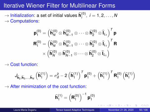
→ Initialization: a set of initial values h(0)i , i = 1,2, . . . ,N
→ Computations:
p(0)1 =
(h(0)
N ⊗ h(0)N−1 ⊗ · · · ⊗ h(0)
2 ⊗ IL1
)Tp
R(0)1 =
(h(0)
N ⊗ h(0)N−1 ⊗ · · · ⊗ h(0)
2 ⊗ IL1
)TR
×(
h(0)N ⊗ h(0)
N−1 ⊗ · · · ⊗ h(0)2 ⊗ IL1
)→ Cost function:
Jh2,h3,...,hN
(h(1)
1
)= σ2
d − 2(
h(1)1
)Tp(0)
1 +(
h(1)1
)TR(0)
1
(h(1)
1
)→ After minimization of the cost function:
h(1)1 =
(R(0)
1
)−1p(0)
1
Laura-Maria Dogariu Tensor-based Adaptive Techniques November 21-26, 2020 56 / 108
→ Computations:
p(1)2 =
(h(0)
N ⊗ h(0)N−1 ⊗ · · · ⊗ h(0)
3 ⊗ IL2 ⊗ h(1)1
)Tp
R(1)2 =
(h(0)
N ⊗ h(0)N−1 ⊗ · · · ⊗ h(0)
3 ⊗ IL2h(1)1
)TR
×(
h(0)N ⊗ h(0)
N−1 ⊗ · · · ⊗ h(0)3 ⊗ IL2h(1)
1
)→ Cost function:
Jh1,h3,...,hN
(h(1)
2
)= σ2
d − 2(
h(1)2
)Tp(1)
2 +(
h(1)2
)TR(1)
2
(h(1)
2
)→ After minimization of the cost function:
h(1)2 =
(R(1)
2
)−1p(1)
2
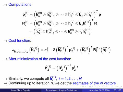
→ Similarly, we compute all h(1)i , i = 1,2, . . . ,N
→ Continuing up to iteration n, we get the estimates of the N vectors
Laura-Maria Dogariu Tensor-based Adaptive Techniques November 21-26, 2020 57 / 108

Simulation Setup
input signals - independent AR(1), obtained by filtering WGNsignals through a first-order system 1/
(1− 0.9z−1)
w(n) - AWGN, with variance σ2w = 0.01
Performance measures:
→ Normalized projection misalignment (NPM) [Morgan et al., IEEESignal Processing Letters, July 1998]:
NPM[hi , hi ] = 1−[
hTi hi
‖hi (n)‖‖hi‖
]2
, i = 1,2, . . . ,N
→ Normalized misalignment (NM):
NM[f, f] = ‖f−f‖2
‖f‖2
Laura-Maria Dogariu Tensor-based Adaptive Techniques November 21-26, 2020 58 / 108

0 20 40 60
Samples
-0.1
0
0.1
0.2
Am
plit
ud
e
(a)
-2
-1
0
1
Am
plit
ud
e
(b)
0 2 4 6 8
Samples
0
0.5
1
Am
plit
ud
e
(c)
1 2 3 4
Samples
-2
-1
0
1
2A
mp
litu
de
(d)
1 2 3 4
Samples
Figure 22: Impulse responses used in simulations: (a) h1 oflength L1 = 32 [Digital Network Echo Cancellers, ITU-TRecommendations G.168, 2002.], (b) h2 of length L2 = 8(randomly generated), (c) h3 of length L3 = 4 (evaluated ash3,l3
= 0.5l3−1, l3 = 1, 2, . . . , L3), (d) h4 of length L4 = 4,(e) h5 of length L5 = 4, and (f) h6 of length L6 = 4 (randomlygenerated).
0 1000 2000 3000 4000 5000 6000 7000 8000
Samples
-0.8
-0.6
-0.4
-0.2
0
0.2
0.4
0.6
0.8
Am
plit
ud
e
Figure 23: The global impulse responseh = h4 ⊗ h3 ⊗ h2 ⊗ h1, of length L = L1L2L3L4 = 8192.
Laura-Maria Dogariu Tensor-based Adaptive Techniques November 21-26, 2020 59 / 108

0 1 2 3 4 5 6 7 8 9
Iterations
-60
-40
-20
0
20
40
60
NM
(dB
)Iterative Wiener filter, M = 500
Conventional Wiener filter, M = 500
Iterative Wiener filter, M = 2500
Conventional Wiener filter, M = 2500
Iterative Wiener filter, M = 5000
Conventional Wiener filter, M = 5000
Iterative Wiener filter, M = 10000
Conventional Wiener filter, M = 10000
Figure 24: Normalized misalignment of the iterative Wiener filter, for differentvalues of M (available data samples to estimate the statistics), for theidentification of the global impulse response from Fig. 23. The input signalsare of type AR(1).
Laura-Maria Dogariu Tensor-based Adaptive Techniques November 21-26, 2020 60 / 108
0 2 4 6 8
Iterations
-50
-40
-30
-20
-10
0
NP
M (
dB
)
(a)
M = 500
M = 2500
M = 5000
M = 10000
2 4 6 8
Iterations
-60
-40
-20
0
NP
M (
dB
)
(b)
M = 500
M = 2500
M = 5000
M = 10000
0 2 4 6 8
Iterations
-80
-60
-40
-20
0
NP
M (
dB
)
(c)
M = 500
M = 2500
M = 5000
M = 10000
0 2 4 6 8
Iterations
-60
-50
-40
-30
-20
-10
NP
M (
dB
)
(d)
M = 500
M = 2500
M = 5000
M = 10000
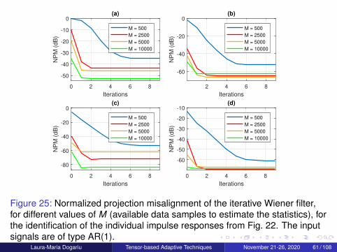
Figure 25: Normalized projection misalignment of the iterative Wiener filter,for different values of M (available data samples to estimate the statistics), forthe identification of the individual impulse responses from Fig. 22. The inputsignals are of type AR(1).
Laura-Maria Dogariu Tensor-based Adaptive Techniques November 21-26, 2020 61 / 108
0 10 20 30
Samples
-0.1
0
0.1
0.2
Am
plit
ud
e
(a)
-2
0
2
Am
plit
ud
e
(b)
0 2 4 6 8
Samples
0
0.5
1
Am
plit
ud
e
(c)
1 2 3 4
Samples
-2
0
2
Am
plit
ud
e
(d)
1 2 3 4
Samples
0
0.5
1
Am
plit
ud
e
(e)
1 1.5 2
Samples
-2
0
2
Am
plit
ud
e
(f)
1 1.5 2
Samples
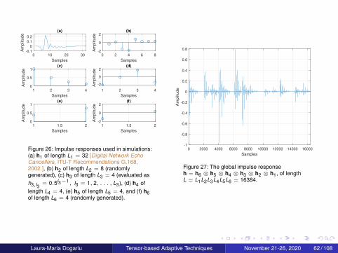
Figure 26: Impulse responses used in simulations:(a) h1 of length L1 = 32 [Digital Network EchoCancellers, ITU-T Recommendations G.168,2002.], (b) h2 of length L2 = 8 (randomlygenerated), (c) h3 of length L3 = 4 (evaluated ash3,l3
= 0.5l3−1, l3 = 1, 2, . . . , L3), (d) h4 oflength L4 = 4, (e) h5 of length L5 = 4, and (f) h6of length L6 = 4 (randomly generated).
0 2000 4000 6000 8000 10000 12000 14000 16000
Samples
-1
-0.8
-0.6
-0.4
-0.2
0
0.2
0.4
0.6
0.8
Am
plit
ud
e
Figure 27: The global impulse responseh = h6 ⊗ h5 ⊗ h4 ⊗ h3 ⊗ h2 ⊗ h1, of lengthL = L1L2L3L4L5L6 = 16384.
Laura-Maria Dogariu Tensor-based Adaptive Techniques November 21-26, 2020 62 / 108
0 1 2 3 4 5 6 7 8 9
Iterations
-60
-40
-20
0
20
40
60
NM
(dB
)Iterative Wiener filter, M = 1000
Conventional Wiener filter, M = 1000
Iterative Wiener filter, M = 2500
Conventional Wiener filter, M = 2500
Iterative Wiener filter, M = 5000
Conventional Wiener filter, M = 5000
Iterative Wiener filter, M = 10000
Conventional Wiener filter, M = 10000
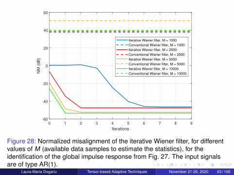
Figure 28: Normalized misalignment of the iterative Wiener filter, for differentvalues of M (available data samples to estimate the statistics), for theidentification of the global impulse response from Fig. 27. The input signalsare of type AR(1).
Laura-Maria Dogariu Tensor-based Adaptive Techniques November 21-26, 2020 63 / 108

2 4 6 8
Iterations
-50
0
NP
M (
dB
)
(a) M = 1000
M = 2500
M = 5000
M = 10000
2 4 6 8
Iterations
-60
-40
-20
NP
M (
dB
)
(b) M = 1000
M = 2500
M = 5000
M = 10000
0 2 4 6 8
Iterations
-80
-60
-40
-20
NP
M (
dB
)
(c) M = 1000
M = 2500
M = 5000
M = 10000
0 2 4 6 8
Iterations
-80
-60
-40
-20
NP
M (
dB
)
(d) M = 1000
M = 2500
M = 5000
M = 10000
2 4 6 8
Iterations
-80-60-40-20
NP
M (
dB
)
(e) M = 1000
M = 2500
M = 5000
M = 10000
0 2 4 6 8
Iterations
-100-80-60-40-20
NP
M (
dB
)
(f)M = 1000
M = 2500
M = 5000
M = 10000
Figure 29: Normalized projection misalignment of the iterative Wiener filter,for different values of M (available data samples to estimate the statistics), forthe identification of the individual impulse responses from Fig. 26. The inputsignals are of type AR(1).
Laura-Maria Dogariu Tensor-based Adaptive Techniques November 21-26, 2020 64 / 108
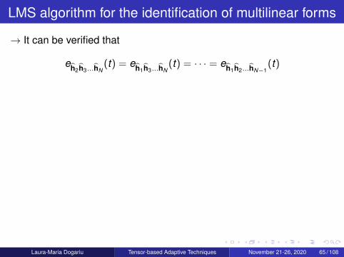
LMS algorithm for the identification of multilinear forms
→ It can be verified that
eh2h3...hN(t) = eh1h3...hN
(t) = · · · = eh1h2...hN−1(t)
LMS-MF updates:
h1(t) = h1(t − 1) + µh1xh2h3...hN
(t)eh2h3...hN(t)
h2(t) = h2(t − 1) + µh2xh1h3...hN
(t)eh1h3...hN(t)
...
hN(t) = hN(t − 1) + µhNxh1h2...hN−1
(t)eh1h2...hN−1(t)
→ µhi> 0, i = 1,2, . . . ,N: step-size parameters
Laura-Maria Dogariu Tensor-based Adaptive Techniques November 21-26, 2020 65 / 108
NLMS-MF
For non-stationary signals: it may be more appropriate to usetime-dependent step-sizes µhi
(t)
A posteriori error signals:
εh2h3...hN(t) = d(t)− hT
1 (t)xh2h3...hN(t)
εh1h3...hN(t) = d(t)− hT
2 (t)xh1h3...hN(t)
...
εh1h2...hN−1(t) = d(t)− hT
N(t)xh1h2...hN−1(t)
Laura-Maria Dogariu Tensor-based Adaptive Techniques November 21-26, 2020 66 / 108

NLMS-MF
By cancelling the a posteriori error signals⇒ NLMS-MF:
h1(t) = h1(t − 1) +αh1
xh2h3...hN(t)eh2h3...hN
(t)
δh1+ xT
h2h3...hN(t)xh2h3...hN
(t)
h2(t) = h2(t − 1) +αh2
xh1h3...hN(t)eh1h3...hN
(t)
δh2+ xT
h1h3...hN(t)xh1h3...hN
(t)
...
hN(t) = hN(t − 1) +αhN
xh1h2...hN−1(t)eh1h2...hN−1
(t)
δhN+ xT
h1h2...hN−1(t)xh1h2...hN−1
(t)
Laura-Maria Dogariu Tensor-based Adaptive Techniques November 21-26, 2020 67 / 108
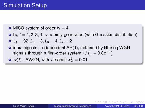
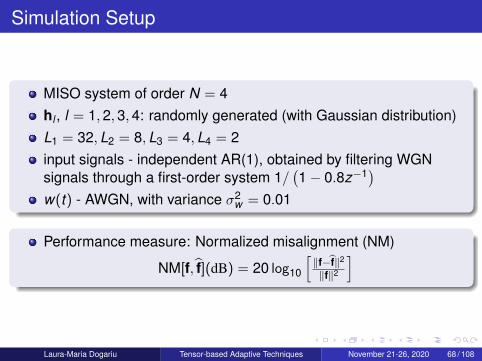
Simulation Setup
MISO system of order N = 4hl , l = 1,2,3,4: randomly generated (with Gaussian distribution)L1 = 32,L2 = 8,L3 = 4,L4 = 2input signals - independent AR(1), obtained by filtering WGNsignals through a first-order system 1/
(1− 0.8z−1)
w(t) - AWGN, with variance σ2w = 0.01
Performance measure: Normalized misalignment (NM)
NM[f, f](dB) = 20 log10
[‖f−f‖2
‖f‖2
]
Laura-Maria Dogariu Tensor-based Adaptive Techniques November 21-26, 2020 68 / 108

Iterations ×104
0 5 10 15
Norm
aliz
ed m
isalig
nm
ent (d
B)
-60
-50
-40
-30
-20
-10
0
LMS-MF
LMS
Figure 30: Normalized misalignment of the LMS-MF and LMS algorithms.The inputs are AR(1) processes, L1L2L3L4 = 2048 and σ2
w = 0.01.
Laura-Maria Dogariu Tensor-based Adaptive Techniques November 21-26, 2020 69 / 108
Iterations ×104
0 5 10 15
Norm
aliz
ed m
isalig
nm
ent (d
B)
-60
-50
-40
-30
-20
-10
0
NLMS-MF
NLMS
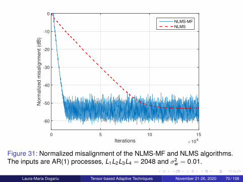
Figure 31: Normalized misalignment of the NLMS-MF and NLMS algorithms.The inputs are AR(1) processes, L1L2L3L4 = 2048 and σ2
w = 0.01.
Laura-Maria Dogariu Tensor-based Adaptive Techniques November 21-26, 2020 70 / 108

Outline
1 Introduction
2 Bilinear Forms
3 Trilinear Forms
4 Multilinear Forms
5 Nearest Kronecker Product Decomposition and Low-RankApproximation
6 An Adaptive Solution for Nonlinear System Identification
7 Conclusions
8 Summary of ContributionsLaura-Maria Dogariu Tensor-based Adaptive Techniques November 21-26, 2020 71 / 108

Nearest Kronecker Product Decomposition andLow-Rank Approximation
Motivation:System identification is very difficult in case of long length impulseresponses (slow convergence, high complexity, low accuracy of thesolution)Bilinear and trilinear forms are only applicable to perfectlyseparable systemsMany echo paths are sparse in nature⇒ low-rank systems
Idea: decompose such high-dimension system identificationproblems into low-dimension problems combined togetherSolution:
Nearest Kronecker product decompositionLow-rank approximation, to decrease computational complexity
Laura-Maria Dogariu Tensor-based Adaptive Techniques November 21-26, 2020 72 / 108

Kalman filter based on the NKP decomposition
h: unknown system of length L = L1L2, L1 ≥ L2
Reshape h into an L1 × L2 matrix: H =[
s1 s2 . . . sL2
]→ sl , l = 1,2, . . . ,L2: short impulse responses of length L1 eachApproximate h by h2 ⊗ h1, where h1: length L1, h2: length L2
Performance measure: M (h1,h2) =‖h−h2⊗h1‖2‖h‖2
=‖H−h1hT
2 ‖F‖H‖F
MinimizeM⇐⇒ find the nearest rank-1 matrix to H: SVDAfter computations, the NKP decomposition of h is:
h(t) =∑P
p=1 h2,p(t)⊗ h1,p(t)Equivalent forms of the error signal:
e1(t) = d(t)−∑P
p=1 hT1,p(t − 1)x2,p(t) = d(t)− h
T1 (t − 1)x2(t)
e2(t) = d(t)−∑P
p=1 hT2,p(t − 1)x1,p(t) = d(t)− h
T2 (t − 1)x1(t)
Original system (length L1L2)⇒ 2 shorter filters (lengths PL1, PL2)⇒ Kalman filter based on the NKP decomposition (KF-NKP)
Laura-Maria Dogariu Tensor-based Adaptive Techniques November 21-26, 2020 73 / 108

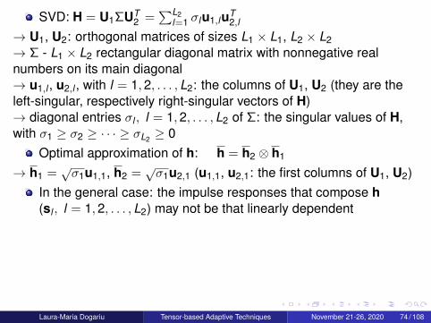
SVD: H = U1ΣUT2 =
∑L2l=1 σlu1,luT
2,l
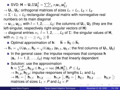
→ U1, U2: orthogonal matrices of sizes L1 × L1, L2 × L2→ Σ - L1 × L2 rectangular diagonal matrix with nonnegative realnumbers on its main diagonal→ u1,l , u2,l , with l = 1,2, . . . ,L2: the columns of U1, U2 (they are theleft-singular, respectively right-singular vectors of H)→ diagonal entries σl , l = 1,2, . . . ,L2 of Σ: the singular values of H,with σ1 ≥ σ2 ≥ · · · ≥ σL2 ≥ 0
Optimal approximation of h: h = h2 ⊗ h1
→ h1 =√σ1u1,1, h2 =
√σ1u2,1 (u1,1, u2,1: the first columns of U1, U2)
In the general case: the impulse responses that compose h(sl , l = 1,2, . . . ,L2) may not be that linearly dependentSolution: use the approximationh ≈
∑Pp=1 h2,p ⊗ h1,p = vec
(H1HT
2), P ≤ L2
→ h1,p, h2,p: impulse responses of lengths L1 and L2→ H1 =
[h1,1 h1,2 . . . h1,P
], H2 =
[h2,1 h2,2 . . . h2,P
]:
matrices of sizes L1 × P and L2 × P
Laura-Maria Dogariu Tensor-based Adaptive Techniques November 21-26, 2020 74 / 108

SVD: H = U1ΣUT2 =
∑L2l=1 σlu1,luT
2,l
→ U1, U2: orthogonal matrices of sizes L1 × L1, L2 × L2→ Σ - L1 × L2 rectangular diagonal matrix with nonnegative realnumbers on its main diagonal→ u1,l , u2,l , with l = 1,2, . . . ,L2: the columns of U1, U2 (they are theleft-singular, respectively right-singular vectors of H)→ diagonal entries σl , l = 1,2, . . . ,L2 of Σ: the singular values of H,with σ1 ≥ σ2 ≥ · · · ≥ σL2 ≥ 0
Optimal approximation of h: h = h2 ⊗ h1
→ h1 =√σ1u1,1, h2 =
√σ1u2,1 (u1,1, u2,1: the first columns of U1, U2)
In the general case: the impulse responses that compose h(sl , l = 1,2, . . . ,L2) may not be that linearly dependentSolution: use the approximationh ≈
∑Pp=1 h2,p ⊗ h1,p = vec
(H1HT
2), P ≤ L2
→ h1,p, h2,p: impulse responses of lengths L1 and L2→ H1 =
[h1,1 h1,2 . . . h1,P
], H2 =
[h2,1 h2,2 . . . h2,P
]:
matrices of sizes L1 × P and L2 × P
Laura-Maria Dogariu Tensor-based Adaptive Techniques November 21-26, 2020 74 / 108
SVD: H = U1ΣUT2 =
∑L2l=1 σlu1,luT
2,l
→ U1, U2: orthogonal matrices of sizes L1 × L1, L2 × L2→ Σ - L1 × L2 rectangular diagonal matrix with nonnegative realnumbers on its main diagonal→ u1,l , u2,l , with l = 1,2, . . . ,L2: the columns of U1, U2 (they are theleft-singular, respectively right-singular vectors of H)→ diagonal entries σl , l = 1,2, . . . ,L2 of Σ: the singular values of H,with σ1 ≥ σ2 ≥ · · · ≥ σL2 ≥ 0
Optimal approximation of h: h = h2 ⊗ h1
→ h1 =√σ1u1,1, h2 =
√σ1u2,1 (u1,1, u2,1: the first columns of U1, U2)
In the general case: the impulse responses that compose h(sl , l = 1,2, . . . ,L2) may not be that linearly dependent
Solution: use the approximationh ≈
∑Pp=1 h2,p ⊗ h1,p = vec
(H1HT
2), P ≤ L2
→ h1,p, h2,p: impulse responses of lengths L1 and L2→ H1 =
[h1,1 h1,2 . . . h1,P
], H2 =
[h2,1 h2,2 . . . h2,P
]:
matrices of sizes L1 × P and L2 × P
Laura-Maria Dogariu Tensor-based Adaptive Techniques November 21-26, 2020 74 / 108
SVD: H = U1ΣUT2 =
∑L2l=1 σlu1,luT
2,l
→ U1, U2: orthogonal matrices of sizes L1 × L1, L2 × L2→ Σ - L1 × L2 rectangular diagonal matrix with nonnegative realnumbers on its main diagonal→ u1,l , u2,l , with l = 1,2, . . . ,L2: the columns of U1, U2 (they are theleft-singular, respectively right-singular vectors of H)→ diagonal entries σl , l = 1,2, . . . ,L2 of Σ: the singular values of H,with σ1 ≥ σ2 ≥ · · · ≥ σL2 ≥ 0
Optimal approximation of h: h = h2 ⊗ h1
→ h1 =√σ1u1,1, h2 =
√σ1u2,1 (u1,1, u2,1: the first columns of U1, U2)
In the general case: the impulse responses that compose h(sl , l = 1,2, . . . ,L2) may not be that linearly dependentSolution: use the approximationh ≈
∑Pp=1 h2,p ⊗ h1,p = vec
(H1HT
2), P ≤ L2
→ h1,p, h2,p: impulse responses of lengths L1 and L2→ H1 =
[h1,1 h1,2 . . . h1,P
], H2 =
[h2,1 h2,2 . . . h2,P
]:
matrices of sizes L1 × P and L2 × P
Laura-Maria Dogariu Tensor-based Adaptive Techniques November 21-26, 2020 74 / 108

Performance measure: M (H1,H2) =‖H−H1HT
2 ‖F‖H‖F
Optimal solutions:H1 =
[h1,1 h1,2 . . . h1,P
]=[√σ1u1,1
√σ2u1,2 . . .
√σPu1,P
]H2 =
[h2,1 h2,2 . . . h2,P
]=[√σ1u2,1
√σ2u2,2 . . .
√σPu2,P
]→ u1,p,u2,p, p = 1,2, . . . ,P: the first P columns of U1, U2
Optimal approximation of h:h(P) =
∑Pp=1 h2,p ⊗ h1,p =
∑Pp=1 σpu2,p ⊗ u1,p
→ the exact decomposition is obtained for P = L2→ if rank(H) = P < L2 (i.e., σi = 0, for P < i ≤ L2)⇒ h can beestimated at least as well as in the conventional approach→ if P is reasonably low as compared to L2 ⇒ important decreasein complexity
Laura-Maria Dogariu Tensor-based Adaptive Techniques November 21-26, 2020 75 / 108
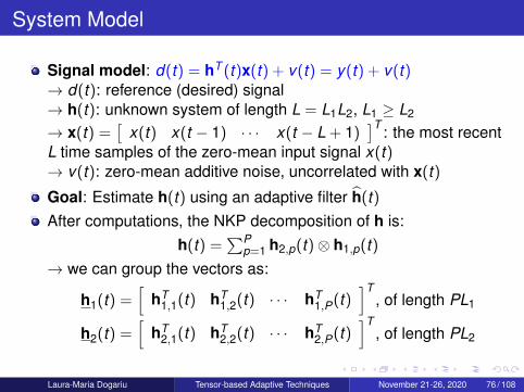
System Model
Signal model: d(t) = hT (t)x(t) + v(t) = y(t) + v(t)→ d(t): reference (desired) signal→ h(t): unknown system of length L = L1L2, L1 ≥ L2
→ x(t) =[
x(t) x(t − 1) · · · x(t − L + 1)]T : the most recent
L time samples of the zero-mean input signal x(t)→ v(t): zero-mean additive noise, uncorrelated with x(t)
Goal: Estimate h(t) using an adaptive filter h(t)After computations, the NKP decomposition of h is:
h(t) =∑P
p=1 h2,p(t)⊗ h1,p(t)→ we can group the vectors as:
h1(t) =[
hT1,1(t) hT
1,2(t) · · · hT1,P(t)
]T, of length PL1
h2(t) =[
hT2,1(t) hT
2,2(t) · · · hT2,P(t)
]T, of length PL2
Laura-Maria Dogariu Tensor-based Adaptive Techniques November 21-26, 2020 76 / 108

Error signal: e(t) = d(t)− y(t) = d(t)− hT (t − 1)x(t)NKP decomposition of the estimated filter:
h(t) =∑P
p=1 h2,p(t)⊗ h1,p(t)
→ h2,p(t)⊗ h1,p(t) =[h2,p(t)⊗ IL1
]h1,p(t) =
[IL2 ⊗ h1,p(t)
]h2,p(t)
→ notations:[h2,p(t − 1)⊗ IL1
]Tx(t) not.
= x2,p(t)[IL2 ⊗ h1,p(t − 1)
]Tx(t) not.
= x1,p(t)→ we can group the vectors as:
h1(t) =[
hT1,1(t) hT
1,2(t) · · · hT1,P(t)
]T
x2(t) =[
xT2,1(t) xT
2,2(t) · · · xT2,P(t)
]T
h2(t) =[
hT2,1(t) hT
2,2(t) · · · hT2,P(t)
]T
x1(t) =[
xT1,1(t) xT
1,2(t) · · · xT1,P(t)
]T
Laura-Maria Dogariu Tensor-based Adaptive Techniques November 21-26, 2020 77 / 108

Kalman filter based on the NKP decomposition
Equivalent forms of the error signal:
e1(t) = d(t)−∑P
p=1 hT1,p(t − 1)x2,p(t) = d(t)− h
T1 (t − 1)x2(t)
e2(t) = d(t)−∑P
p=1 hT2,p(t − 1)x1,p(t) = d(t)− h
T2 (t − 1)x1(t)
Original system (length L1L2)⇒ 2 shorter filters (lengths PL1, PL2)
Kalman filter based on the NKP decomposition:h1(t) = h1(t − 1) + k1(t)e1(t) h2(t) = h2(t − 1) + k2(t)e2(t)
→ k1(t),k2(t): Kalman gain vectors:
k1(t) = Rm1(t)x2(t)[xT
2 (t)Rm1(t)x2(t) + σ2v]−1
k2(t) = Rm2(t)x1(t)[xT
1 (t)Rm2(t)x1(t) + σ2v]−1
Laura-Maria Dogariu Tensor-based Adaptive Techniques November 21-26, 2020 78 / 108
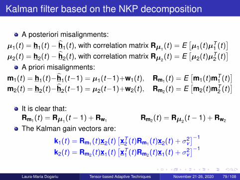
Kalman filter based on the NKP decomposition
A posteriori misalignments:µ1(t) = h1(t)− h1(t), with correlation matrix Rµ1
(t) = E[µ1(t)µT
1 (t)]
µ2(t) = h2(t)− h2(t), with correlation matrix Rµ2(t) = E
[µ2(t)µT
2 (t)]
A priori misalignments:m1(t) = h1(t)−h1(t−1) = µ1(t−1)+w1(t), Rm1(t) = E
[m1(t)mT
1 (t)]
m2(t) = h2(t)−h2(t−1) = µ2(t−1)+w2(t), Rm2(t) = E[m2(t)mT
2 (t)]
It is clear that:Rm1(t) = Rµ1
(t − 1) + Rw1 Rm2(t) = Rµ2(t − 1) + Rw2
The Kalman gain vectors are:
k1(t) = Rm1(t)x2(t)[xT
2 (t)Rm1(t)x2(t) + σ2v]−1
k2(t) = Rm2(t)x1(t)[xT
1 (t)Rm2(t)x1(t) + σ2v]−1
Laura-Maria Dogariu Tensor-based Adaptive Techniques November 21-26, 2020 79 / 108

Computational Complexity
P
2 4 6 8 10 12 14 16 18 20
Mu
ltip
lica
tio
ns
×105
2
4
6
8
(a)
KF-NKP, L1 = 25, L
2 = 20
KF, L = 500
P
5 10 15 20 25 30
Mu
ltip
lica
tio
ns
×106
1
2
3
4
(b)
KF-NKP, L1 = 32, L
2 = 32
KF, L = 1024
Figure 32: Number of multiplications (per iteration) required by the KF-NKP and KF, as afunction of P. The KF-NKP uses two shorter filters of lengths PL1 and PL2 (with P ≤ L2), whilethe length of the KF is L = L1L2: (a) L1 = 25, L2 = 20, and (b) L1 = L2 = 32.
Laura-Maria Dogariu Tensor-based Adaptive Techniques November 21-26, 2020 80 / 108
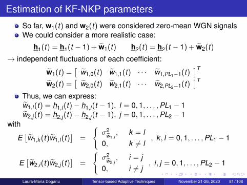
Estimation of KF-NKP parameters
So far, w1(t) and w2(t) were considered zero-mean WGN signalsWe could consider a more realistic case:
h1(t) = h1(t − 1) + w1(t) h2(t) = h2(t − 1) + w2(t)
→ independent fluctuations of each coefficient:
w1(t) =[
w1,0(t) w1,1(t) · · · w1,PL1−1(t)]T
w2(t) =[
w2,0(t) w2,1(t) · · · w2,PL2−1(t)]T
Thus, we can express:w1,l(t) = h1,l(t)− h1,l(t − 1), l = 0,1, . . . ,PL1 − 1w2,j(t) = h2,j(t)− h2,j(t − 1), j = 0,1, . . . ,PL2 − 1
with
E[w1,k (t)w1,l(t)
]=
{σ2
w1,l, k = l
0, k 6= l, k , l = 0,1, . . . ,PL1 − 1
E[w2,i(t)w2,j(t)
]=
{σ2
w2,j, i = j
0, i 6= j, i , j = 0,1, . . . ,PL2 − 1
Laura-Maria Dogariu Tensor-based Adaptive Techniques November 21-26, 2020 81 / 108
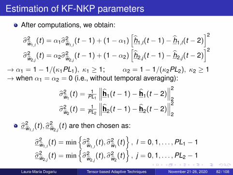
Estimation of KF-NKP parameters
After computations, we obtain:
σ2w1,l
(t) = α1σ2w1,l
(t − 1) + (1− α1)[h1,l(t − 1)− h1,l(t − 2)
]2
σ2w2,j
(t) = α2σ2w2,j
(t − 1) + (1− α2)[h2,j(t − 1)− h2,j(t − 2)
]2
→ α1 = 1− 1/(κ1PL1), κ1 ≥ 1; α2 = 1− 1/(κ2PL2), κ2 ≥ 1→ when α1 = α2 = 0 (i.e., without temporal averaging):
σ2w1
(t) = 1PL1
∥∥∥h1(t − 1)− h1(t − 2)∥∥∥2
2
σ2w2
(t) = 1PL2
∥∥∥h2(t − 1)− h2(t − 2)∥∥∥2
2
σ2w1,l
(t), σ2w2,j
(t) are then chosen as:
σ2w1,l
(t) = min{σ2
w1,l(t), σ2
w1(t)}, l = 0,1, . . . ,PL1 − 1
σ2w2,j
(t) = min{σ2
w2,j(t), σ2
w2(t)}, j = 0,1, . . . ,PL2 − 1
Laura-Maria Dogariu Tensor-based Adaptive Techniques November 21-26, 2020 82 / 108
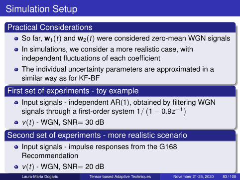
Simulation Setup
Practical ConsiderationsSo far, w1(t) and w2(t) were considered zero-mean WGN signalsIn simulations, we consider a more realistic case, withindependent fluctuations of each coefficientThe individual uncertainty parameters are approximated in asimilar way as for KF-BF
First set of experiments - toy exampleInput signals - independent AR(1), obtained by filtering WGNsignals through a first-order system 1/
(1− 0.9z−1)
v(t) - WGN, SNR= 30 dB
Second set of experiments - more realistic scenarioInput signals - impulse responses from the G168Recommendationv(t) - WGN, SNR= 20 dBLaura-Maria Dogariu Tensor-based Adaptive Techniques November 21-26, 2020 83 / 108

First Set of Experiments
Samples
10 20 30 40 50 60 70 80 90 100
Am
plit
ud
e
-1
0
1
(a)
Samples
10 20 30 40 50 60 70 80 90 100
Am
plit
ud
e
-1
0
1
(b)
Figure 33: Impulse responses of length L = 100, which are decomposed using L1 = L2 = 10:(a) a cluster of 10 samples (alternating the amplitudes 1 and −1) padded with zero, withrank (H) = 1; and (b) the same cluster shifted to the right by 5 samples, so that rank (H) = 2.
Laura-Maria Dogariu Tensor-based Adaptive Techniques November 21-26, 2020 84 / 108
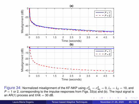
Time (seconds)
0 0.5 1 1.5 2 2.5 3 3.5 4 4.5 5
Mis
alig
nm
ent (d
B)
-60
-40
-20
0(a)
P = 1
P = 2
Time (seconds)
0 0.5 1 1.5 2 2.5 3 3.5 4 4.5 5
Mis
alig
nm
ent (d
B)
-40
-30
-20
-10
0(b)
P = 1
P = 2
Figure 34: Normalized misalignment of the KF-NKP using σ2w1
= σ2w2
= 0, L1 = L2 = 10, andP = 1 or 2, corresponding to the impulse responses from Figs. 33(a) and (b). The input signal isan AR(1) process and SNR = 30 dB.
Laura-Maria Dogariu Tensor-based Adaptive Techniques November 21-26, 2020 85 / 108

Second Set of Experiments
0 100 200 300 400 500
Samples
-0.1
0
0.1
0.2
Am
plit
ude
(a)
0 100 200 300 400 500
Samples
-0.2
-0.1
0
0.1
0.2
Am
plit
ude
(b)
0 200 400 600 800 1000
Samples
-0.4
-0.2
0
0.2
0.4
Am
plit
ude
(c)
Figure 35: Impulse responses used in simulations: (a) the first impulse response from G168Recommendation, with L = 500; (b) the first and the fifth impulse responses (concatenated) fromG168 Recommendation, with L = 500; and (c) acoustic impulse response, with L = 1024.
Laura-Maria Dogariu Tensor-based Adaptive Techniques November 21-26, 2020 86 / 108

P
5 10 15 20
Appro
x. err
or
(dB
)
-100
-80
-60
-40
-20
0(a)
P
5 10 15 20
Appro
x. err
or
(dB
)
-100
-80
-60
-40
-20
0(b)
P
5 10 15 20 25 30
Appro
x. err
or
(dB
)
-100
-80
-60
-40
-20
0(c)
Figure 36: Approximation error (in terms of the normalized misalignment), for the identificationof the impulse responses from Fig. 35: (a) impulse response from Fig. 35(a), of length L = 500,with L1 = 25 and L2 = 20; (b) impulse response from Fig. 35(b), of length L = 500, with L1 = 25and L2 = 20; and (c) impulse response from Fig. 35(c), of length L = 1024, with L1 = L2 = 32.
Laura-Maria Dogariu Tensor-based Adaptive Techniques November 21-26, 2020 87 / 108

Time (seconds)
0 1 2 3 4 5 6
Mis
alig
nm
ent (d
B)
-30
-25
-20
-15
-10
-5
0
KF-NKP, P = 2
KF-NKP, P = 3KF-NKP, P = 4
KF-NKP, P = 5
KF
Figure 37: NM of the KF-NKP (using different values of P) and KF, for the identification of theimpulse response which changes after 3 seconds from Fig. 35(a) to (b). The input signal is anAR(1) process, L = 500, and SNR = 20 dB. The KF-NKP uses L1 = 25, L2 = 20, andσ2
w1= σ2
w2= 10−8; the KF uses the same value of σ2
w .
Laura-Maria Dogariu Tensor-based Adaptive Techniques November 21-26, 2020 88 / 108
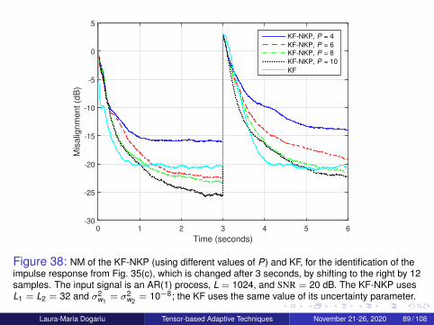
Time (seconds)
0 1 2 3 4 5 6
Mis
alig
nm
ent (d
B)
-30
-25
-20
-15
-10
-5
0
5
KF-NKP, P = 4
KF-NKP, P = 6KF-NKP, P = 8
KF-NKP, P = 10
KF
Figure 38: NM of the KF-NKP (using different values of P) and KF, for the identification of theimpulse response from Fig. 35(c), which is changed after 3 seconds, by shifting to the right by 12samples. The input signal is an AR(1) process, L = 1024, and SNR = 20 dB. The KF-NKP usesL1 = L2 = 32 and σ2
w1= σ2
w2= 10−8; the KF uses the same value of its uncertainty parameter.
Laura-Maria Dogariu Tensor-based Adaptive Techniques November 21-26, 2020 89 / 108
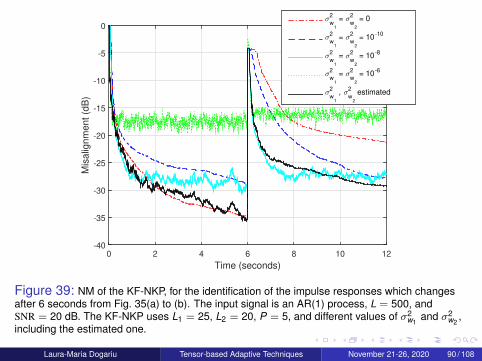
Time (seconds)
0 2 4 6 8 10 12
Mis
alig
nm
ent (d
B)
-40
-35
-30
-25
-20
-15
-10
-5
0σ
2
w1
= σ2
w2
= 0
σ2
w1
= σ2
w2
= 10-10
σ2
w1
= σ2
w2
= 10-8
σ2
w1
= σ2
w2
= 10-6
σ2
w1
, σ2
w2
estimated
Figure 39: NM of the KF-NKP, for the identification of the impulse responses which changesafter 6 seconds from Fig. 35(a) to (b). The input signal is an AR(1) process, L = 500, andSNR = 20 dB. The KF-NKP uses L1 = 25, L2 = 20, P = 5, and different values of σ2
w1and σ2
w2,
including the estimated one.
Laura-Maria Dogariu Tensor-based Adaptive Techniques November 21-26, 2020 90 / 108

Time (seconds)
0 1 2 3 4 5 6
Mis
alig
nm
ent (d
B)
-30
-25
-20
-15
-10
-5
0
5
KF-NKP, P = 4
KF-NKP, P = 6KF-NKP, P = 8
KF-NKP, P = 10
KF
Figure 40: NM of the KF-NKP (using different values of P) and KF, for the identification of theimpulse response from Fig. 35(c), which is changed after 3 seconds, by shifting to the right by 12samples. The input signal is an AR(1) process, L = 1024, and SNR = 20 dB. The KF-NKP usesL1 = L2 = 32, while the specific parameters σ2
w1and σ2
w2are estimated; the KF uses the
uncertainty parameter estimated as in [Paleologu et al., Proc. IEEE ICASSP, 2014].
Laura-Maria Dogariu Tensor-based Adaptive Techniques November 21-26, 2020 91 / 108
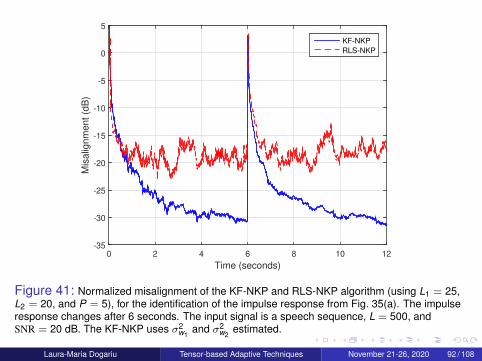
Time (seconds)
0 2 4 6 8 10 12
Mis
alig
nm
ent (d
B)
-35
-30
-25
-20
-15
-10
-5
0
5
KF-NKP
RLS-NKP
Figure 41: Normalized misalignment of the KF-NKP and RLS-NKP algorithm (using L1 = 25,L2 = 20, and P = 5), for the identification of the impulse response from Fig. 35(a). The impulseresponse changes after 6 seconds. The input signal is a speech sequence, L = 500, andSNR = 20 dB. The KF-NKP uses σ2
w1and σ2
w2estimated.
Laura-Maria Dogariu Tensor-based Adaptive Techniques November 21-26, 2020 92 / 108

Time (seconds)
0 2 4 6 8 10 12
Mis
alig
nm
ent (d
B)
-30
-25
-20
-15
-10
-5
0
5
KF-NKP
RLS-NKP
Figure 42: Normalized misalignment of the KF-NKP and RLS-NKP algorithm (usingL1 = L2 = 32 and P = 10), for the identification of the impulse response from Fig. 35(c). Theimpulse response changes after 6 seconds. The input signal is a speech sequence, L = 1024,and SNR = 20 dB. The KF-NKP uses σ2
w1and σ2
w2estimated.
Laura-Maria Dogariu Tensor-based Adaptive Techniques November 21-26, 2020 93 / 108

Outline
1 Introduction
2 Bilinear Forms
3 Trilinear Forms
4 Multilinear Forms
5 Nearest Kronecker Product Decomposition and Low-RankApproximation
6 An Adaptive Solution for Nonlinear System Identification
7 Conclusions
8 Summary of ContributionsLaura-Maria Dogariu Tensor-based Adaptive Techniques November 21-26, 2020 94 / 108

Motivation
Previous methods for nonlinearities identification:→ Volterra-based approach→ Neural networks
Main problem: very high computational complexity
Our solution:→ Compute the Taylor series expansion→ Approximate the function using its first significant Taylor seriescoefficients, neglecting the other ones→ Find the coefficients using an adaptive algorithm
Laura-Maria Dogariu Tensor-based Adaptive Techniques November 21-26, 2020 95 / 108

The Nonlinearities Identification Problem
Figure 43: System model.
→ x : zero mean real valued input signal→ g(x): nonlinear, bijective, odd-type function with the Taylor seriesexpansion of the form g(x) ∼=
∑Mk=1(gkxk )
→ d(n) = gT x(n) + w(n): system output, corrupted by AWGN→ e(n) = d(n)− gT x(n) = (gT − gT
)x(n) + w(n): output error
Laura-Maria Dogariu Tensor-based Adaptive Techniques November 21-26, 2020 96 / 108

The Nonlinearities Identification Problem
Goal - obtain an estimation of the coefficient vector:g(n) = [g1(n), g2(n), ..., gM(n)]T
Criterion to minimize - mean-square error (MSE):
J(n) = E [e2(n)] = σ2d − 2gT p + gT Rg, where
→ σ2d = E [d2(n)] - desired signal variance
→ p = E [x(n)d(n)] - cross-covariance between the input signalx(n) and the desired signal d(n)→ R = E [x(n)xT (n)] - covariance matrix of the vector x(n)
Wiener-Hopf solution: go = R−1pProblems: → the system should be time-invariant
→ statistical expectations need to be known
Laura-Maria Dogariu Tensor-based Adaptive Techniques November 21-26, 2020 97 / 108

The Adaptive Approach
Least-Mean-Square (LMS) solution:g(n) = g(n − 1) + µx(n)ea(n)
→ ea(n) = d(n)− gT(n − 1)x(n): a priori error
→ µ: step-size parameter
Normalized LMS (NLMS) solution:µ(n) = α
||x(n)||2+δ
→ α: normalized step-size (0 < α < 2)→ δ: regularization parameter
Laura-Maria Dogariu Tensor-based Adaptive Techniques November 21-26, 2020 98 / 108
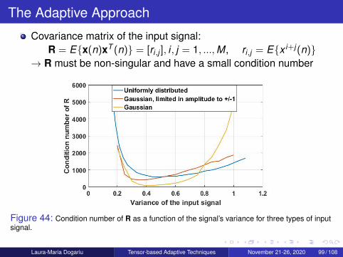
The Adaptive Approach
Covariance matrix of the input signal:R = E{x(n)xT (n)} = [ri,j ], i , j = 1, ...,M, ri,j = E{x i+j(n)}
→ R must be non-singular and have a small condition number
Figure 44: Condition number of R as a function of the signal’s variance for three types of inputsignal.
Laura-Maria Dogariu Tensor-based Adaptive Techniques November 21-26, 2020 99 / 108

Experimental Results
Simulation Setup:NLMS filter of length M = 6Input: the first M powers of a zero mean Gaussian signal, limitedin amplitude to ±1Functions to be identified: → g(x) = x + 0.3x3 + 0.2x5
→ g(x) = arctan(ax),0 < a < 1
Analyze:Coefficients’ valuesFunction’s reconstruction
Laura-Maria Dogariu Tensor-based Adaptive Techniques November 21-26, 2020 100 / 108

Figure 45: Evolution of the coefficients gk computed using the NLMSalgorithm for the polynomial function g(x) = x + 0.3x3 + 0.2x5. The blackdotted lines are the actual coefficients.
Laura-Maria Dogariu Tensor-based Adaptive Techniques November 21-26, 2020 101 / 108

Figure 46: Representation of the polynomial function and the reconstructedfunction when the input x ∈ [−1; 1].
Laura-Maria Dogariu Tensor-based Adaptive Techniques November 21-26, 2020 102 / 108
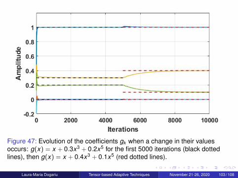
Figure 47: Evolution of the coefficients gk when a change in their valuesoccurs: g(x) = x + 0.3x3 + 0.2x5 for the first 5000 iterations (black dottedlines), then g(x) = x + 0.4x3 + 0.1x5 (red dotted lines).
Laura-Maria Dogariu Tensor-based Adaptive Techniques November 21-26, 2020 103 / 108
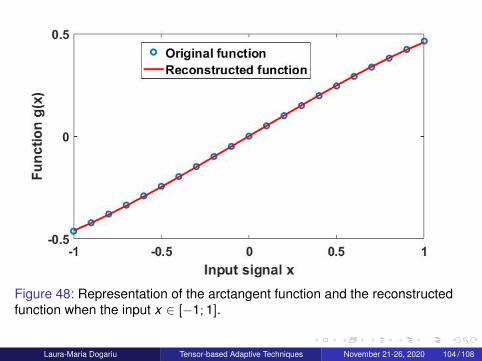
Figure 48: Representation of the arctangent function and the reconstructedfunction when the input x ∈ [−1; 1].
Laura-Maria Dogariu Tensor-based Adaptive Techniques November 21-26, 2020 104 / 108

Outline
1 Introduction
2 Bilinear Forms
3 Trilinear Forms
4 Multilinear Forms
5 Nearest Kronecker Product Decomposition and Low-RankApproximation
6 An Adaptive Solution for Nonlinear System Identification
7 Conclusions
8 Summary of ContributionsLaura-Maria Dogariu Tensor-based Adaptive Techniques November 21-26, 2020 105 / 108

Conclusions
Contributions in the area of multilinear system identificationMultilinearity is defined in relation to the individual impulseresponses composing the systemThe systems are modeled using tensorsNKP decomposition and low-rank approximation for systemswhich are not perfectly separableAn adaptive method for nonlinear systems (with smallnonlinearities)Numerous applications, since most real-world systems arenonlinear
Laura-Maria Dogariu Tensor-based Adaptive Techniques November 21-26, 2020 106 / 108

Thank you!
Part of this work was supported by a grant of the Romanian Ministry of Education and
Research, CNCS – UEFISCDI, project number: PN-III-P1-1.1-PD-2019-0340, within
PNCDI III.
Laura-Maria Dogariu Tensor-based Adaptive Techniques November 21-26, 2020 107 / 108

Outline
1 Introduction
2 Bilinear Forms
3 Trilinear Forms
4 Multilinear Forms
5 Nearest Kronecker Product Decomposition and Low-RankApproximation
6 An Adaptive Solution for Nonlinear System Identification
7 Conclusions
8 Summary of ContributionsLaura-Maria Dogariu Tensor-based Adaptive Techniques November 21-26, 2020 108 / 108