TEN THEOREMS ABOUT QUANTUM MECHANICAL ...

Physica A 153 (1988) 97-113 North-Holland, Amsterdam

TEN THEOREMS ABOUT QUANTUM MECHANICAL MEASUREMENTS

N.G. VAN KAMPEN Institute for Theoretical Physics of the University, Utrecht, The Netherlands

Received 1 July 1988

The aim of quantum mechanics is to explain macroscopic, objectively recorded phenomena. Microscopic objects are measured by enabling them to interact with a macroscopic measuring apparatus prepared in a metastable state. Macroscopic objects, such as cats, are not above the laws of quantum mechanics, but owing to their enormously dense level spectrum other aspects than single eigenvalues and eigenfunctions are prominent. These aspects can be described in classical terms, such as probabilities instead of probability amplitudes. The measuring act is fully described by the Schrodinger equation for object system and apparatus together. The collapse of the wave function is a consequence rather than an additional postulate. A model is constructed to demonstrate these statements. It also appears that the entropies of the object system and the apparatus increase by the same amount, namely the entropy difference between the metastable initial state and the stable final state of the apparatus.

1. Formulation of the problem

Many a theory in physics makes use of mathematical entities that do not correspond to an intuitively understandable physical object. Of course intuition can be educated; as a consequence some of these entities, for instance energy, become so familiar as to be regarded as concrete objects. Others, such as the coordinates xF in general relativity, remain abstract without anybody worrying about it. A third class, however, of which entropy is an example, remains a source of bewilderment and controversy. The most notorious member of this class is the wave function #. It is an indispensable tool for quantum mechanical calculations, but its connection with actually observed phenomena is remote. This connection is the subject of the continuing debate about the foundations of quantum mechanics and the theory of measurement [l-4]. A huge literature has been provoked by the question: How exactly does the wave function $ relate to the phenomena that I can observe and measure?

Meanwhile quantum mechanics is in daily use and is extremely successful in understanding, predicting, and computing these same phenomena. One knows

037%4371/88/$03.50 0 Elsevier Science Publishers B.V. (North-Holland Physics Publishing Division)

98 N.G. van Kampen I Ten theorems about quantum mechanical measurements

how to handle $ so as to get concrete, observable conclusions about the physical world. Apparently the problem is solved in practice; the difficulties enter only when one starts philosophizing. This philosophizing has given rise to a number of “interpretations”, in which (I/ is endowed with more physical significance than is needed for the actual calculation of the phenomena. There are a number of schools with different views, including such mind-boggling fantasies as the many-world interpretation [5], which go far beyond the world of physical phenomena.

My question is: How is it possible that, in spite of these differences of opinion, quantum mechanics is used in practice to obtain uncontroversial results? The purpose of this article is not to defend some interpretation, but to analyze what happens when quantum mechanics is used to obtain results that can be compared with experiments. This is a matter of physics; what I say is true or false - not the expression of a philosophical view about the deeper meanings of reality.

It is not surprising that some of my conclusions are the same as those of Bohr [6] inasmuch as his aim too was to understand how the quantum mechanical formalism works. Yet in some crucial points the present description of the theory of measurement differs from what is usually regarded as the Copenhagen interpretation. A great help in elucidating the measuring process is the explicit model constructed in section 6. I repeat that I shall avoid all philosophical extrapolations of the physical facts. Znterpretationes non @fingo.

2. Preliminary remarks about quantum mechanics

Theorem I: Quantum mechanics works.

It describes and computes those phenomena for which it was invented, such as black body radiation and spectra; and numerous others, such as specific heat and superconductivity. All these phenomena are macroscopic, objective, and permanently recorded, for instance on a photographic plate or as a table in the Physical Review. Hence

Theorem ZZ: Quantum mechanics is concerned with macroscopic phenomena, which are not perturbed by observation.

The familiar stories about the influence of the observer on the system do not apply to real observations in a laboratory. They apply to a world of lilliputians, where an observer is able to aim at a single gamma quantum at a preassigned electron. Such stories may be helpful in exposing the difference with the

N. G. van Kampen I Ten theorems about quantum mechanical measurements 99

classical picture of particles and waves, but they are irrelevant for the

observations as done in practice. Our purpose is merely to know how to deal with actually observed phenomena.

One example of such phenomena is the diffraction of a beam of electrons passing through a crystal. In order to compute the observed diffraction pattern one makes use of a quantity $, called the “wave function of a single electron”. The value of [I)[ *, multiplied by the number N of electrons in the beam, is the observed blackening of the photographic plate. The value of [$I* for a single electron does occur in the calculation, but is not observed itself. One may call it the probability density of the electron, but that is merely a name for the observed blackening divided by N.

Theorem ZZZ: The quantum mechanical probability is not observed but merely

serves as an intermediate stage in the computation of an observable phenomenon,

The old question: Does $ refer to a single system or to an ensemble? - must therefore be answered as follows. I,!J is a mathematical object pertaining to a single system; its square [$I2 may be called a single system probability. However, in order to confront this quantity with reality one must do observations on a large number of similar systems, in such a way that the probability density materializes as an actual density.

Not only the probability I+/*, but also the wave function $ itself occurs merely as a mathematical tool in the calculation of spectra, collision cross- sections, etc. It does not occur in the result that can be handed to the experimenter for comparison with the real world. This situation is similar with the way in which the relativistic coordinates n’ are used, and also the vector potential in Maxwell theory. For some reason, however, it is the wave function that has been the object of numerous speculations concerning its “true nature”. Everybody is free to speculate, but

Theorem ZV: Whoever endows I,!I with more meaning than is needed for computing observable phenomena is responsible for the consequences.

He has the duty to show that his speculations do not lead to contradictions, and preferably that they are of some use (other than agreement with precon- ceived philosophical views). If he does not succeed he should not blame quantum mechanics.

Such theories are usually carefully constructed so as to reproduce the known results of quantum mechanics; they can therefore neither be verified nor falsified by experiments. One might hope that they are simpler or easier to


handle but actually they are usually complicated and contrived. This is particularly so when they fail to respect the superposition principle and as a result lose the tool of transforming in Hilbert space. But I digress: our purpose is merely to see how quantum mechanics works in practice.

3. The measuring process according to von Neumann

Any measuring arrangement corresponds with the measurement of an observable quantity represented by a Hermitian operator A. Such an operator has a complete set of eigenfunctions x,, with eigenvalues h,,

AX, = Ax,, .

For convenience we suppose that the eigenvalues are discrete and nondegener- ate and that the x, are normalized. Von Neumann gives the following abstract description of the measuring process [7].

(i) As long as no measurement occurs the system is described by a wave function G(t), which evolves according to the Schrodinger equation for the system.

(ii) Suppose at t, the system is brought into contact with an apparatus for measuring A. Then the possible outcomes are the values A,. The probability for finding h, is

pm = I(xmlv4t,>)l”~

(In this connection the measurement is always taken to be instantaneous, i.e., short on the time scale of the Schrodinger evolution.)

(iii) If the value A, has been found by the measurement the wave function changes abruptly from $(t,) into x,,. This sudden reduction or collapse of the wave function is to be added as a new postulate to the Schrodinger quantum mechanics. (Incidentally, this collapse can be used to prepare a system in a certain state x,.)

(iv) It is necessary that the measuring apparatus is left in a state from which the observer can see that the result was A m: a pointer on a dial must point at m.

However, to read this result I need another apparatus, which by a second measuring process determines the position of the pointer. And this process is repeated and gives rise to a chain of measurements, which can end only in the brain of the observer, where in some mysterious way it becomes a part of the “gedankliche Innerleben des Individuums”.

This is actually the conclusion of von Neumann and others [7,8]. I find it

N.G. van Kampen I Ten theorems about quantum mechanical measurements 101

hard to understand that someone who arrives at such a conclusion does not seek the error in his argument. Quantum mechanics is not a theory of the mind of an observer, but of physical, objectively recorded phenomena, see theorem II. The question is how $ relates to spectra or specific heats; the mind of the observer is irrelevant. Moreover the answer was already known to Bohr: the quantum mechanical measurement is terminated when the outcome has been macroscopically recorded.

4. Macroscopic systems

A macroscopic system, such as a certain amount of a gas, a crystal, or a pointer on a volt meter, is composed of a huge number of particles. As a consequence its energy levels lie inordinately dense on any energy scale used in the laboratory. The typical distance SE between two successive levels is much and much smaller than the inaccuracy AE of the best energy measurement by the best experimenter. Hence such a system can never be prepared in a single eigenstate of the energy operator. (In fact, if it were in a single eigenstate it would behave as one big molecule in a stationary state; no particle could be seen to move!) Rather, the wave function $ of a macroscopic system is always a superposition of an enormous number (namely AE/6E) of eigenstates. A macroscopic system does obey the laws of quantum mechanics, but the familiar

picture of individual eigenvalues and eigenstates is no longer adequate. Other features become prominent; they constitute the subject matter of macroscopic physics [9, lo]. (A loose analogy within the realm of classical theory is formed by statistical mechanics: A many-body system has features, such as pressure and temperature, which do not exist for a few particles; they are the subject matter of thermodynamics.)

The wave function Cc, of a macroscopic system describes all its individual particles and their movements. It obeys a gigantic Schrodinger equation as long as the system is not perturbed, not even by a measuring apparatus. This $, however, is the “microstate” of the system. When an experimenter prides himself that he has prepared the system in a well-defined state, he refers to the macrostate. He does not pretend to know its Hilbert vector @, he only knows that it lies in a certain subspace of Hilbert space with BE/SE dimensions.

When a macroscopic pointer indicates a macroscopic point on a dial the number of microscopic eigenstates involved has been estimated by Bohm [ll] to be 105’. When the observer shines in light in order to read the position of the pointer, the photons do perturb the $ of the pointer, but the perturbation does not affect the macrostate. The vector $ is moved around a bit in these 10” dimensions but its components outside the subspace remain negligible. That is

102 N.G. van Kampen i Ten theorems about quantum mechanical measurements

the reason why macroscopic observations can be recorded objectively, in- dependently of the observations and the observer, and may therefore be the object of scientific study. The lilliputian measurements of Heisenberg [12] and von Neumann do not apply to experiments with macroscopic systems.

A typically macroscopic feature is the existence of thermodynamic equilibrium states. Those are macrostates which the system, when left alone, will reach sooner or later. Certain systems possess metastable states as well, for example supersaturated vapor. A metastable state is a macrostate in which the system can reside for a long time before its ultimate transition into the stable equilibrium state. In many cases, however, this transition can be triggered by a minute perturbation, even a single microscopic particle. That is the way in which microscopic particles can be recorded macroscopically, as in the Wilson chamber, the Geiger counter and the AgBr crystals of the photographic plate.

Theorem V: A quantum mechanical measuring apparatus consists of a macroscopic system prepared in a metastable state.

The transition from the metastable into the stable macrostate provides the free energy needed to make the microscopic phenomena macroscopically visible. It is also the reason why the measuring process is irreversible (camp. theorem X) and therefore permanently recorded.

5. Schriidinger’s cat

This much discussed paradox [13] consists of a cat locked in a black box together with a radioactive sample. Moreover there is a Geiger counter, which on being triggered by an emitted alpha particle activates a device that kills the cat. The argument runs as follows. After some time the whole system is in a superposition of two states: one in which no decay has occurred that triggered the mechanism and one in which it has occurred. Hence the state of the cat also consists of a superposition of two states.

Icat) = allife) + bldeath) . (4

There are two coefficients a, b (in general complex), which depend on the time elapsed. The state remains a superposition until an observer looks at the cat. Then, according to section 3, the wave function (2) collapses into either (life) or [death) with respective probabilities 1 aI2 and 1 b12.

If this is not sufficiently paradoxical one may consider an observer who has a friend who does the experiment for him [S]. At which moment does the wave

N. G. van Kampen I Ten theorems about quantum mechanical measurements 103

function collapse, when the friend looks at the cat or when he communicates his finding to the observer? This quandary must be resolved by anybody who regards JI as a physical object rather than a tool for computing macroscopic phenomena.

To make the paradoxical nature of (2) more explicit suppose that the observer decides to observe another quantity than the question of life and death, for instance the temperature of the cat (i.e., the total kinetic energy of its molecules). The expectation value of such a quantity G is

(G) = ~cz~~G,, + lb12Gdd + a*bGpd + ab*G,, ,

where G,, etc. are the matrix elements of G. This expectation value is not a statistical average of the value G,, and G,, with probabilities 1 aI2 and 1 b12, but contains cross terms between life and death.

The answer to this paradox is again that the cat is macroscopic. Life and death are macrostates comprising an enormous number of eigenstates 18) and Id) respectively. Any wave function of the cat has the form

Icat) = c a,lC) + c b,ld) . e d

The cross terms in the expression for ( G) are

,c, a*,b,G,, + 2 a,b:G,, . e,d

(3)

As there is such a wealth of terms, all with different phases and magnitudes, they mutually cancel and (3) practically vanishes. This is the way in which the typical quantum mechanical interference become inoperative between macrostates. As a result (G) now does appear as a statistical average.

Theorem VI: The wave function of a system of a macroscopic number of particles gives, on measuring macroscopic quantities, results that can be described in terms of classical probabilities. [9]

One remark concerning microscopic systems, such as a single elementary particle, must be added. In the region of high quantum numbers such a system behaves with respect to measurements as a macroscopic system. The reason is again that there are many eigenstates within the margin AE of macroscopic accuracy. Readers who think that they have found a counterexample to theorem V, for instance the Cerenkov counter, have made use of this fact. A particle that betrays its position through Cerenkov radiation thereby changes

104 N.G. van Kampen 1 Ten theorems about quantum mechanical measurements

its microscopic $ but not its macrostate. Its energy changes by an amount 6E but not AE.

6. A model for a measuring apparatus

We shall construct a measuring apparatus for observing the position of an electron. More precisely, our apparatus will be able to tell whether the electron has passed through some preassigned region U in space. It could be used for instance in the double slit experiment to decide through which slit the electron has passed. We shall find that such an observation does indeed destroy the interference pattern. All this is a consequence of the Schriidinger equation for the total system, which consists of the object system, in this case the electron, together with the apparatus. There is no need to supplement the Schrodinger evolution with an additional postulate, as in the theory of von Neumann.

Our apparatus [14] consists of an atom together with the electromagneticfield. The apparatus is macroscopic because of the many degrees of freedom embodied in the normal modes of the field*. We label the modes by their wave vector k and for simplicity ignore polarization. The Hilbert space of the apparatus is the direct product of the Hilbert space of the atom and the space of all possible excitations of the field modes. The stable equilibrium is the state with the atom and all modes in their ground states. A metastable state can be made by putting the atom in an excited state, for instance 2S, from which no transition to the ground state through emission of a photon is allowed. When, however, an electron appears in the neighborhood of the atom its Coulomb interaction distorts the 2s state so as to create a dipole moment, which makes the transition possible. Such a transition is irreversible and leaves a permanent record of the passage of the electron. For instance the emitted photon can be caught on a photographic plate or in a counter. One may regard the plate or the counter as part of the measuring apparatus if one wishes, but the crucial point is that, once the photon has been emitted, the presence of the electron has been permanently recorded.

The only states of the apparatus that we need for our purpose are I+ ; 0) (atom excited, no photons) and I- ; k) ( a om t in ground state, one photon k). The wave function ?P of the total system (electron + apparatus) is a linear superposition, whose coefficients are elements of the Hilbert space of the electron:

q(t) = cp(r, t)l+; 0) + C $k(r, 41-i k) . k

* In the model of Peres [15] the measuring apparatus is not explicitly macroscopic, but instead a noisy perturbation is put in by hand.


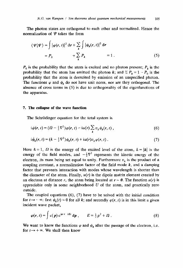
The photon states are orthogonal to each other and normalized. Hence the normalization of !P takes the form

P, is the probability that the atom is excited and no photon present; Pk is the probability that the atom has emitted the photon k; and C Pk = 1 - PO is the probability that the atom is deexcited by emission of an unspecified photon. The functions cp and $k do not have unit norm, nor are they orthogonal. The absence of cross terms in (5) is due to orthogonality the apparatus.

7. The collapse of the wave function

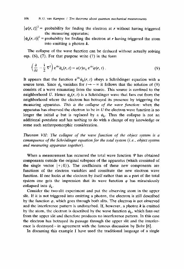
The Schrodinger equation for the total system is

@@, ‘) = (’ - iv2)(P@, t, - i”(r) T U,@k(rY t, ,

i$k(r, t) = (k - $V2)rCl,(r, t) + iu(r)u,cp(r, t) .

Here 6 = 1, 0 is the energy of the excited level of

of the eigenfunctions of

(6)

(7)

the atom, k = Ikl is the energy of the field modes, and - iv’ represents the kinetic energy of the electron, its mass being set equal to unity. Furthermore uk is the product of a coupling constant, a normalization factor of the field mode k, and a damping factor that prevents interaction with modes whose wavelength is shorter than the diameter of the atom. Finally, U(T) is the dipole matrix element created by an electron at distance r, the atom being located at r = 0. The function U(T) is appreciable only in some neighborhood U of the atom, and practically zero outside.

The coupled equations (6), (7) h ave to be solved with the initial condition for t+ - 03: first Gk(t) = 0 for all k; and secondly rp(r, t) is in this limit a given incident wave packet,

(P(I-, t) = I

c(p) eiP’r-iE’ dp ,

We want to know the functions cp for t+ + 00. We shall then know

E=ip2+t. (8)

and t+Qk after the passage of the electron, i.e.


1 cp(r, t)l* = probability for finding the electron at r without having triggered the measuring apparatus;

I&(‘, t)j2 = probability for finding the electron at r having triggered the atom into emitting a photon k.

The collapse of the wave function can be deduced without actually solving eqs. (6), (7). For that purpose write (7) in the form

It appears that the function eikt&(r, t) obeys a Schrodinger equation with a source term. Since & vanishes for t-+ - 00 it follows that the solution of (9) consists of a wave emanating from the source. This source is confined to the neighborhood U. Hence +Gk(r, t) is a Schrodinger wave that fans out from the neighborhood where the electron has betrayed its presence by triggering the measuring apparatus. This is the collapse of the wave function: when the apparatus has observed the electron to be in U the electron wave function is no longer the initial cp but is replaced by a J/k. Thus the collapse is not an additional postulate and has nothing to do with a change of my knowledge or some such anthropomorphic consideration.

Theorem VII: The collapse of the wave function of the object system is a consequence of the Schrtidinger equation for the total system (i.e., object system and measuring apparatus together).

When a measurement has occurred the total wave function P has obtained components outside the original subspace of the apparatus (which consisted of the single vector I+; 0)). The coefficients of these new components are functions of the electron variables and constitute the new electron wave function. If one looks at the electron by itself rather than as a part of the total system one gets the impression that its wave function cp has miraculously collapsed into ICI,.

Consider the two-slit experiment and put the observing atom in the upper slit. If it is not triggered into emitting a photon, the electron is still described by the function cp, which goes through both slits. The electron is not observed and the interference pattern is undisturbed. If, however, a photon k is emitted by the atom, the electron is described by the wave function &, which fans out from the upper slit and therefore produces no interference pattern. In this case the electron has betrayed its passage through the upper slit and the interference is destroyed - in agreement with the famous discussion by Bohr [6].

In discussing this example I have used the traditional language of a single


electron and its probability distribution. The same result can be formulated operationally in agreement with theorem III. The actual experiment consists in shooting a succession of electrons at the two slits. For each single electron I write down its position on the receiving screen and record whether or not a photon has been emitted. After finishing the experiment I sit down at my desk with my notes, collect the events without photon and mark their positions on a piece of paper. The marks will produce an interference pattern. When I do the same for the events that were accompanied by a photon no interference appears on the paper.

If the atom were absent the wave function of the electron would be the cp given by (8), modified by the boundary conditions on the two-slit screen. In the presence of the atom cp is the solution of the coupled equations (6), (7) with the same boundary conditions and with (8) as initial condition. These two functions cp are not quite the same; the apparatus influences the electron even without detecting it. The interference pattern we obtained by selecting the undetected electrons is not quite the same as the one obtained when no attempt is made to detect them. The physicist says that the atom is polarizable, or that it makes a virtual transition to the ground state. If one wants the electron to be able to act on the measuring apparatus one cannot avoid a reaction. Yet the fact that an apparatus affects the wave function of the object system even when the measurement is not successful has caused some debate

W921.

8. Probability and density matrix

The classical probability of some feature of a system is defined as the number of elementary states that have that feature, divided by the total number of possible elementary states. The elementary states are supposed to have equal probabilities, or else to have given a priori probabilities. Probability calculus is merely the technique of transforming one probability distribution into another. The physical input is the specification of the elementary states and their a priori probabilities. This input depends on my knowledge - or rather lack of knowledge - because actually the system can be in no more than one state. If I have cast two dice without looking, the probability that the total number of points equals 10 is &; the moment I look at one die the probability jumps to either 0 or a, depending on what I see; and once I have looked at both the probability is 0 or 1.

Quantum mechanical probabilities, however, are equal to I~/J[’ by definition, see section 2. They are not defined by means of an underlying set of possible states (which, by the way, would also require a postulate about a priori


probabilities). There is no cogent reason to insist that it should be possible to interpret them in this classical way. Obstinate attempts to construct such a “stochastic interpretation” have not met with success [17]. At any rate they are irrelevant for our purpose of understanding how quantum mechanics works in practice.

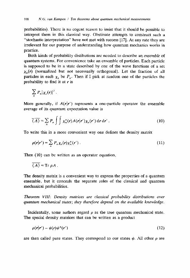
Both kinds of probability distibutions are needed to describe an ensemble of quantum systems. For convenience take an ensemble of particles. Each particle is supposed to be in a state described by one of the wave functions of a set x,(r) (normalized but not necessarily orthogonal). Let the fraction of all particles in each x, be P,,. Then if I pick at random one of the particles the probability to find it at r is

More generally, if A(rlr’) represents a one-particle operator the ensemble average of its quantum expectation value is

(A) = c P, /I xE(r)A(rlr’)x,(r’) dr dr’ . n (10)

To write this in a more convenient way one defines the density matrix

drlr’) = F P,x,(r)xE (4 . (11)

Then (10) can be written as an operator equation,

(A)=TrpA.

The density matrix is a convenient way to express the properties of a quantum ensemble, but it conceals the separate roles of the classical and quantum mechanical probabilities.

Theorem VIII: Density matrices are classical probability distributions over quantum mechanical states; they therefore depend on the available knowledge.

Incidentally, some authors regard p as the true quantum mechanical state. The special density matrices that can be written as a product

drlr’) = +WlCr*W (12)

are then called pure states. They correspond to our states I,!J. All other p are


mixed states, that is what we would call the states of an ensemble. These authors should not be surprised that their quantum systems have states that depend on the author’s knowledge.

9. Application to the measurement process

Suppose the measurement process of section 3 is applied to a particle in a state +(r). Before measurement the density matrix has the form (12). After the measurement is performed, but before I look at the result, the density matrix is

P, being given by (1). After I have looked and found a certain result A, the density matrix is reduced to p2(rlr’) = x,(r)xz(r’). This reduction of p1 to p2 is classical and not more mysterious than the reduction of the probability distribution of the dice upon looking at them.

The reduction of p into pl, however, is due to the collapse of the wave function caused by the interaction with the measuring apparatus. This can be shown explicitly for the model in section 6. Let A be an operator acting on the electron alone. Its expectation value in the state (4) is

(13)

This cannot be written as the expectation value of A in an electron wave function, but only by means of a density matrix in the electron space:

(WA1 W) = Tr 0,

where

This shows that after a measurement the object system cannot be described by a 1(1 but only by a p, as if it were an ensemble. The reason is that it is still part of the total system, which includes the apparatus whose state is here left unspecified.

If one does look at the apparatus and finds that no photon has been emitted, the electron does have a wave function, namely q(r); or properly normalized,

camp. (5)

110 N. G. van Kampen I Ten theorems about quantum mechanical measurements

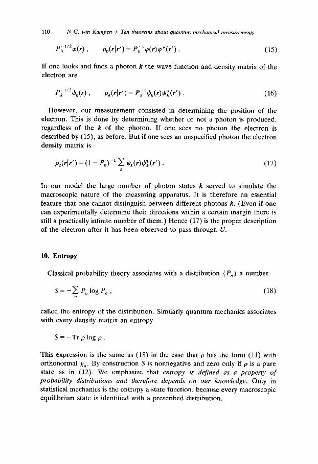
If one looks and finds a photon k the wave function and density matrix of the electron are

However, our measurement consisted in determining the position of the electron. This is done by determining whether or not a photon is produced, regardless of the k of the photon. If one sees no photon the electron is described by (15), as before. But if one sees an unspecified photon the electron density matrix is

(17)

In our model the large number of photon states k served to simulate the macroscopic nature of the measuring apparatus. It is therefore an essential feature that one cannot distinguish between different photons k. (Even if one can experimentally determine their directions within a certain margin there is still a practically infinite number of them.) Hence (17) is the proper description of the electron after it has been observed to pass through U.

10. Entropy

Classical probability theory associates with a distribution {P,} a number

s=-CPJogP,, n

(18)

called the entropy of the distribution. Similarly quantum mechanics associates with every density matrix an entropy

S=-Trplogp.

This expression is the same as (18) in the case that p has the form (11) with orthonormal x,. By construction S is nonnegative and zero only if p is a pure state as in (12). We emphasize that entropy is defined as a property of probability distributions and therefore depends on our knowledge. Only in statistical mechanics is the entropy a state function, because every macroscopic equilibrium state is identified with a prescribed distribution.


We apply the entropy concept to our model for the measuring process. First of all one sees immediately:

Theorem IX: The total system is described throughout by the wave vector W and

has therefore zero entropy at all times.

This ought to put an end to speculations about measurements being responsible for increasing the entropy of the universe. (It won’t, of course.)

Secondly, before the measuring operation the electron itself is described by a vector in its own Hilbert space, viz. (S), and has therefore also zero entropy. The apparatus has zero entropy as well since it is in the pure state I+ ; 0). (This is a special feature of our simple example; usually one does not have complete knowledge of the prepared state of the apparatus.)

After the measurements, if I do not look at the outcome, the entropy is the one associated with the density matrix (14). If I do look and find no photon the electron is in the pure state 9 with zero entropy. If I look and find an unspecified photon the entropy is the one associated with (17).

To compute this entropy we note that it can be expressed in the eigenvalues pu, of the matrix (17) by

s=-Cf-Ql~gPv. (19) Y

The equation for the eigenvalues p and corresponding eigenfunctions t(r) is

d(r) = _/ p,(rlr’)S(r’) dr’ = Cl- pJ1 T rclk(r) 1 Icr:(r’)Kr’> dr’ . (20)

Multiply this equation with @i,(r) and integrate

Here

ffk = rLi (Mr) dr

and

Mkfk = (1 - P,-,)r _/ $,,*,(r)ek(r) dr .

(21)

Thus the eigenvalues of (20) are also eigenvalues of M,.,. (This is not true for


those s(r) for which all (Ye vanish, but in that case the eigenvalue p of (20) is also zero and does not contribute to the entropy (10) anyway.) Hence the CL, in (19) may be taken to be the eigenvalues of M. Incidentally, it follows that one might write S = -Tr M log M.

We shall now prove that this is equal to the increase of the entropy of the measuring apparatus. We start from the density matrix of the total system after the emission of an unspecified photon has been observed:

The density matrix of the apparatus is obtained by taking the trace over the electron states,

This is an operator in the space of one-photon states. Its eigenvalues are easily obtained with the aid of the orthonormality of the photon states ( - ; k) . They turn out to be identical with the eigenvalues p,, of the matrix M found in (21).

Theorem X: The measurement operation increases the entropies of the object system and of the apparatus by equal amounts.

This increase is due to the incomplete specification of their final states. It is equal to the thermodynamic entropy difference between the stable and metastable macrostates of the apparatus.

References

[l] M. Jammer, The Philosophy of Quantum Mechanics (Wiley, New York, 1974), chap. 11.

B. d’Espagnat, Conceptual Foundations of Quantum Mechanics, 2nd ed. (Benjamin, Read-

ing, MA, 1976), part 4.

[2] Quantum Theory and Measurement, a collection of reprints edited by J.A. Wheeler and W.H. Zurek (Princeton University Press, Princeton, NJ, 1983).

L.E. Ballentine, Am. J. Phys. 55 (1987) 785.

[3] K. Baumann and R.U. Sexl, Die Deutungen der Quantentheorie (Vieweg, Braunschweig,

1984).

[4] J. Gribbin, In search of Schrodinger’s Cat. (Corgi Books, Transworld Publishers, London,

1984).

E. Squires, The Mystery of the Quantum World (Hilger, Bristol, 1986).

[5] H. Everett, Rev. Mod. Phys. 29 (1957) 454.

J.A. Wheeler, Rev. Mod. Phys. 29 (1957) 463.

B.S. de Witt, Physics Today 20, No. 9 (Sept., 1970) 30.


[6] N. Bohr, in: Albert Einstein, Philosopher-Scientist, I. P.A. Schilp, ed. (Harper and Row, New York, 1949). W. Heisenberg, in: Niels Bohr and the Development of Physics, W. Pauli, L. Rosenfeld and V. Weisskopf, eds. (Pergamon, London, 1955). H. Stapp, Am. .I. Phys. 40 (1972) 1098.

(71 J. von Neumann, Mathematische Grundlagen der Quantentheorie (Springer, Berlin, 1931). F. London and E. Bauer, La thtorie de l’observation en mecanique quantique (Hermann, Paris, 1939). C. Cohen-Tannoudji, B. Diu and F. Laloi, Mecanique quantique I (Hermann, Paris, 1973), p. 216.

[8] E.P. Wigner, Symmetries and Reflections (Indiana Univ. Press, Bloomington, 1967), p. 171. Reprinted in ref. [2].

[9] N.G. van Kampen, Physica 20 (1954) 603; Fortschritte der Physik 4 (1956) 405. [lo] G. Ludwig, Z. Phys. 150 (1958) 346; 152 (1958) 98.

A. Daneri, A. Loinger and G.M. Prosperi, Nucl. Phys. 33 (1962) 297. [ll] D. Bohm, Quantum Theory (Prentice-Hall, New York, 1951), chap. 4. [12] W. Heisenberg, Die physikalischen Prinzipien der Quantentheorie (Hirzel, Leipzig, 1930),

chap. II. [13] E. Schriidinger, Naturwissenschaften 23 (1935) 807, 823, 844. Reprinted in ref. [3], translated

in ref. [2]. A. Peres, Found. of Phys. 14 (1984) 1131. L.E. Ballentine, Am. J. Phys. 54 (1986) 947.

[14] N.G. van Kampen, Philips Res. Repts. 30 (1975) p. 65*; in: Quantum Measurement and Chaos,E.R. Pike and S. Sarkar, eds. (Plenum, New York, 1987).

[15] A. Peres, Am. J. Phys. 54 (1986) 688. [16] M. Renninger, Z. Phys. 136 (1953) 251; 158 (1960) 417. [17] D. Bohm, Phys. Rev. 85 (1952) 166, 180.

D. Bohm, B.J. Hiley, and P.N. Kaloyerou, Phys. Rep. 144 (1987) 321. L. de Broglie and J.P. Vigier, La theorie quantique restera-t-elle indeterministe? (Gauthier- Villars, Paris, 1953). E. Nelson, Quantum Fluctuations (Princeton Univ. Press, Princeton, NJ, 1985). F.J. Belinfante, A. Survey of Hidden-Variables Theories (Pergamon, Oxford, 1973).

TEN THEOREMS ABOUT QUANTUM MECHANICAL ...

Documents

Transcript of TEN THEOREMS ABOUT QUANTUM MECHANICAL ...