136 TRANSPORTATION RESEARCH RECORD 1297

Temporal Effects of Incidents on Transit Ridership in Orange County, California ERIK FERGUSON

Aggregate level transit ridership forecasting models often are based on time series data, with potential serial autocorrelation properties that can bias parameter estimates upward and error estimates downward , and skew forecasting confidence intervals and their resulting interpretation significantly. A combined time series and cross-sectional regression model of transit ridership is developed that incorporates temporal variations as well as supply, demand, and pricing characteristics of the market for transit ser­vices in Orange County, California, between 1973 and 1989. It was found that Orange County transit ridership exhibits signifi­cant serial and seasonal fluctuations, which were captured in the model. The temporary and lingering effects of incidents were also tested. The 1979 oil shortage was shown to have a large positive impact on transit ridership , which dwindled quite rapidly once the oil shortage ended . A work stoppage of 6 weeks' duration in 1981 had a large negative impact on transit ridership, which dwin­dled only slowly. A shorter work stoppage in 1986, during which limited service was provided by transit agency administrative pe r­sonnel, had a much smaller negalive imp::ic1 lhan the 1981 work stoppage, which dwindled much more rapidly . Trnnsit fare and gasoline pricing variables were found to have no significant effect on transit ridership in the preferred temporally based model. Transit fares did not increase much in real terms over the period covered, and did not reflect variations in transit service provided, being predicated on a simple county-wide flat fare basis. Over 70 percent of all Orange County transit riders were captive riders in 1987, having no car available to them for commuting or other travel purposes, making the price of gasoline basically irrelevant to the majority of such transit riders in the shorter term.

Many problem in urban and regional transportation analysis have imp rtant temporal dimensions. Foreca ·ting changes in employment, population, or travel behavior are just a few examples of ;ire;is where temporal processes and interactions may be important in identifying existing conditions, explain­ing past tr nds, or forecasting future outcome of urban and regional policies and planning. Time series analysis is one method of explicitly incorporating temporal phenomena in regression analysis for forecasting purposes. Time series anal­ysis often ili used as a projection me thod, based exclusively on the past performance f specific exogenous output varia­bles . Policy input variables, such as spatial or socioecon mic variations in demand, often are not included in time series models, because of lack of data, lack of analysis software, or both.

Cross-sectional models typically provide more opportuni­ties for testing policy sensitivity. However, pa_rameters and

nfidence interval estimated in cross-sectional mod ls may bia ed ·ignificantly, if serial amocorrelation i present.

mbined time series and cro · -s ctional models offer tbe

Graduate City Planning Program , College of Architecture , Georgia Institute of Technology , Atlanta, Ga. 30332-0158.

possibility of providing policy sensitivity and controlling for temporal estimation biases simultaneously. Simultaneous time-series and cross-sectional regression analysis are applied to transit ridership forecasting, assuming only first-order, se­rial autoregressive processes are involved (J). Three types of temporal variability are included in this analysis:

1. First-order serially autoregressive impacts; 2. First-order seasonally autoregressive impacts; and 3. Permanent, temporary, and lingering impacts of inci­

dents over time.

Quarterly transit ridership data are used to demonstrate how alternative model formulations can be evaluated in terms of descriptive ability (overall goodness of fit), serial autocor­relation (parameter estimation bias), and predictive ability (forecast error).

First, some of Lhe basic statistical and econometric princi­ples required to conduct an exploratory analysis of this type are described. Second, various transit ridership model vari­ations formulated to test these ideas using original data col­lected in Orange County, California, are compared and con­trasted. Finally, some of the policy and research implications derived from a comparative evaluation of the various model results are reported.

DATA

The data u ·ed in this analysi were taken from the Orange County Transit Di ·trict (0 D) aggregate, or system-wide transit ridership forecasting model. Variations on the tem­poral model discussed here were tested by the author while employed by OCTD from 1986 to 1988. A version of the model discussed here was developed independently by the Center for Economic Research at Chapman College (2), and is now in use by OCTD for transit ridership forecasting pur­poses. The Chapman College model is used to forecast transit ridership in Orange County 5 years in advance for financial and service planning purposes. In addition, the model is used to comply with the requirements of the regional transportation planning process, as administered by OCTD, the Southern

alifornia Association of Governments, the Orange ounty Tran ·portation Commission, the State of California Depart­ment of Transportation, and other responsible public agencies in the region .

OCTD has been in operation for close to 20 years, begin­ning in the fourth quarter of 1973, after the first Arab oil embargo occurred . Quarterly transit ridership data are de-

Ferguson

rived from a unique, stratified random sample of driver trip sheets, and adjusted using method of fare payment and fare data. The accuracy of this data is good, with an expected annual statistical measurement error of not more than ± 2 percent at the 95 percent confidence interval (3). Vehicle service miles, a supply measure, is even more accurate, as the length of all bus runs driven is known, and measured to within the nearest 10th of a vehicle-mile in service. Average county-wide employment figures, used in this analysis both as a reasonable and a reliable proxy measure of demand, are derived from Chapman College's annual forecast of Orange County employment, and are equally reliable in measure­ment. Over half of all person-trips made on the Orange County transit system are work-related trips, with a large part of the remainder school and recreational activities.

All other data used in this analysis are temporal in nature, and are not subject to sampling or measurement errors, at least not in the same sense that the cross-sectional variables just described might be .

METHODOLOGY

A variety of models are described, tested, and compared in this analysis. The principal types of models used include cross­sectional models, first-order autoregressive models (4), com­bined time series and cross-sectional models (5), seasonally adjusted combined models, and incident impact models. Eval­uation measures include the traditional cross-sectional mea­sures of overall goodness-of-fit and the magnitude and direc­tion of independent variable effects, as well as two measures of serial autocorrelation, Durbin-Watson's d (6), for models without lagged endogenous variables (7), and Durbin's h (8), for models with lagged endogenous variables (9) .

Basic Cross-Sectional and Time-Series Models

A traditional cross-sectional transit ridership forecasting model is as follows:

PAS, = b0 + b1 * VSM, + b2 • EMP, + e, (1)

where

PAS, = total transit ridership in time period I,

VSM, = total vehicle service miles in time period t, EMP, = average service area employment in time pe-

riod t, e, = error in prediction associated with the obser­

vation of total transit ridership in time period t, and

b0 , b1 , b2 = parameters to be estimated.

A slight modification of this equation results in the familiar double-log econometric regression model, which provides di­rect measures of the elasticity of demand for the dependent variable (total transit ridership) with respect to each indepen­dent variable (total vehicle service-miles and average quar­terly employment). The double-log model has proven to be useful for public and private policy sensitivity analysis in a variety of cases, and will be relied on throughout the re­mainder of this analysis :

137

ln(P AS,) = b0 + b, • ln(VSM,) + b2 • ln(EMP,) + e, (2)

If a time series variable, such as quarterly transit ridership, is subject to serial autocorrelation of the error terms in pre­diction , the resulting parameter estimates may be severely biased, with overall goodness of fit measures and parameter standard error terms similarly biased by the existence of serial autocorrelation. A commonly used and powerful test of serial autocorrelation in regression analysis is Durbin-Watson's d:

2: (e, - e,_, 2

d = L (e,)2 (3)

where

d = Durbin-Watson's d, and e, _ 1 = error in prediction associated with the observation

of total transit ridership in the preceding time pe­riod, t - 1.

Values of d around 2 indicate the existence of no significant serial autocorrelation. Values of d close to 0 suggest positive serial autocorrelation, whereas values of d close to 4 suggest negative serial autocorrelation. If significant serial autocor­relation is identified, a lagged endogenous variable may be used to estimate an autoregressive time series regression model, on the basis of a normal first order autoregressive process, as follows:

ln(PAS,) = b0 + b1 • ln(PAS,_ 1) (4)

where PAS, _ 1 is the total transit ridership in the immediately preceding time period, t - 1.

Such a model may still be biased by residual or higher order levels of serial autocorrelation. Durbin-Watson's d does not provide a reliable measure of serial autocorrelation in models that include lagged endogenous variables as independent var­iables. In such cases, Durbin's h may be used in place of Durbin-Watson's d, as a more reliable indicator of serial au­tocorrelation :

[ T ]

112

h = p * l - T • vaT (b.)

where

h = Durbin 's h; p = 1 - d/2;

(5)

T = total number of observations on which the regression model is based (not degrees of free­dom), i.e., sample size; and

var(b.) variance of b. , or square of the estimated stan­dard error term for b., where b. is the parameter estimate of the first-order lagged endogenous variable [In(PAS, _ 1)] , regardless of whether any other serially related exogenous or endogenous variables are included in the model.

A combined time series and cross-sectional transit ridership forecasting model would be as follows:

ln(PAS,) = b0 + b 1 * ln(VSM,) + b2 * ln(EMP,)

+ b3 * In(PAS,_ 1) + e, (6)

138

Other Types of Serial Processes

In addition to first-order autoregressive processes, many other types of serial autocorrelation are theoretically possible. Dif­ferenced models, in which the dependent variable is defined as the difference between ridership in time period t and ri­dership in some previous time period, t - n, may also be relevant in some cases, as are moving-average models, in which the dependent variable is hypothesized to be influenced by the weighted average of transit ridership over several time periods, which may include before and after time periods in estimation.

These analytically more complex types of models require the estimation of error terms in separate models are the use of instrumental variables in estimating final regression equa­tions ( 4). Such models are usually neither necessary nor rel­evant in practice, often do not require direct estimation in any case, and are not further considered here. This implies that the temporal processes influencing aggregate transit rid­ership are relatively simple and straightforward, an assump­tion that will be tested explicitly as part of the development of the final recommended transit ridership forecasting model.

Seasonal Models

A second type of direct serial autocorrelation is seasonal au­toregressivity. In this example, the length of seasonality is 4, because there are four quarters in each year. One formulation of such a seasonal model, which retains a first-order, lagged endogenous variable and cross-sectional variables as before, is as follows:

ln(PAS,) = b0 + b 1 * ln(VSM,) + b2 * ln(EMP,)

+ b, * ln(PAS,_ 1)

+ b4 * ln(PAS,_") + e,

where n is the length of seasonality.

(7)

Alternatively, seasonality may be included in the model through the use of dummy variables. Each seasonal dummy variable tests for differences in transit ridership betweeu Lhal season and an arbitrary reference season, which may be any of the four quarters, as follows:

ln(PAS,) = b0 + b, * ln(VSM,) + b2 • ln(EMP,)

+ b3 * ln(PAS,_ 1) + b4 *SEA,

+ b5 * SEA2 ... + bx* SEA"_, + e, (8)

where SEAx is 1 if the observed total transit ridership or.r.mred in season n, and is 0 otherwise.

The choice of which alternative seasonal model formulation to use may be influenced by the length of seasonality. When the number of seasons (quarters, months , weeks, days, hours, etc.) is relatively small, collinearity between the first-order autoregressive term and the seasonal term will tend to be higher, suggesting the use of seasonal dummy variables. When the number of seasons is relatively high, the loss of efficiency in model estimation because of the necessary inclusion of

TRANSPORTATION RESEARCH RECORD 1297

n - 1 independent variables will tend to be higher, suggesting the use of a seasonally differenced term as an independent variable.

Incident Models

An incident is any event that disturbs the observed relation­ships between a dependent variable and any or all of its as­sociated time-series and cross-sectional explanatory variables. Examples of incidents in the transit industry might include a large scale restructuring of transit services (the introduction of a new rail service, where before there was none, for ex­ample), significant fare restructuring, gas shortages, oil price increases, ambitious marketing programs, and perhaps the classic example, the transit work stoppage, or labor strike (JO). Such incidents may have transit ridership impacts which are positive or negative, abrupt or gradual, temporary or permanent, in nature. A simple model of any or all of these types of effects is as follows:

ln(PAS,) = b0 + b 1 * ln(VSM,) + b2 * ln(EMP,)

+ b1 * INCs * eCs - 1)•5 + e, (9)

where

IN Cs = 1 in time period s, during which the incident ac­tually occurred and in all subsequent time periods as well, 0 otherwise;

s time period, where s is measured in the standard time periods used in model construction, beginning with s = 1 in that time period during which the incident actually occurred; and

o exponential decay parameter, theoretically or em­pirically derived, which provides a measure of the (constant) rate at which an incident's effect changes over time (Table 1).

It is possible thrit ;in inr.in~nt m:iy h;we one level of impact in the time period during which it occurs, and an entirely different level of impact in subsequent time periods. A good example of this is the effect of a work stoppage on transit ridership. It is common knowledge in the transit industry that work stoppages can affect transit ridership long after a strike has ended. While the strike is in progress, no transit service is provided at all, and thus no one may ride transit anywhere in the affected service area. Transit riders must then seek out alternative means of transportation (automobile, walking, etc.), or forgo their customary travel behavior. After the strike ends, individuals may choose to take one or more of the following actions for different types of trips :

1. They may revert immediately to their former customary travel behavior (i.e., get back on the bus);

2. They may permanently change their travel behavior (i.e., purchase a private automobile for their own personal use; or

3. They may delay changing their behavior, but ultimately wind up reverting to their former customary travel behavior

Ferguson 139

TABLE I NUMERICAL RELATIONSHIP BETWEEN DELTA AND INCIDENT EFFECTS

Value of delta (decay factor) Effect of incident over time

Positive Permanent, and increasing over time.

0 Permanent, and constant over time.

Negative Temporary and lingering, that is, decreasing constantly over time.

Negative and very large i.e., negative infinity)

Temporary and abrupt, because the effect v~rnishes immediately, once the stimulus has been removed.

(e.g., to keep up their end of a carpool arrangement for a certain length of time).

Depending on the length and severity of the incident, indi­vidual travellers may wait longer or shorter periods of time before returning to their former customary behavior patterns. It is difficult if not impossible to model different kinds of temporal processes that occur simultaneously, explicitly in the context of time series analysis, just as the effects of separate incidents that occur at the same time cannot be isolated in a single aggregate forecasting model. It is possible to separate the temporary effect of one incident from the more or less permanent aftereffects of that same incident as follows:

ln(P AS,) = b0 + b1 * ln(VSM,) + b2 * ln(EMP,)

where

+ b3 * ln(PASr-1) + b4 *SEA,

+ b5 * SEA2 + b6 * SEA3

+ b7 * INCS + INCs+l * efS - l)•o + e, (10)

IN Cs = 1 in time period s only, when the incident ac­tually occurred, 0 otherwise; and

INCs+ 1 = 1 in time period s + 1, immediately after the incident occurred, and 1 in all subsequent time periods, 0 otherwise.

The analytical results of each of these types of transit ridership forecasting models will be compared in the next section, with conclusions drawn concerning model validity, and their po­tential utility in public policy analysis. The primary data used in the model are shown in Figure 1. Orange County employ­ment increased with few interruptions, from less than 500,000 in 1973 to well over 1,000,000 in 1989. OCTD transit service (VSM) expanded rapidly during the 1970s, but remained vir­tually constant during the 1980s. OCTD ridership nonetheless continued to increase in the 1980s, though at a much lower annual growth rate than in the 1970s.

RESULTS

Analytical results from a variety of model formulations are compared in terms of internal validity. Internal validity is composed of the statistical measures that explain the signif­icance of estimated parameters, and the existence of measure­ment errors associated with collinearity or serial autocorre-

9.2-----9-

8.8-8.6-8.4 -8 2 ~

o 8 ~

g 7.8 -~ 7.6-~ 7.4 -

7.2 .... I. 7 - I

6.8 .... I 6.6 - l

'

---... -

6.4 "'. / / 6. 2 -f, ~ r rrrm--nn-riTr-n-nTTTI' • rrr 11 n t t rrnrnTT1Tl"'Yrn-

1973 1975 1977 1979 198 1 1983 1985 1987 1989 QUARTERLY OBSERVATIONS

- RIDER SH IP VEHICLE SERVICE MILES - - EMPLOYMENT

FIGURE 1 Orange County, California, trends.

Iation. External validity could also be checked by comparing these model results with those from other transit ridership forecasting models, and actual transit performance in future time periods.

Basic Models

Table 2 presents results for basic cross-sectional, autoregres­sive time-series, and combined transit ridership forecasting models. All three models show significant serial autocorre­lation in the distribution of error terms, indicating that model parameters may be biased in terms of magnitude, confidence level, or both. Parameter estimates for the simple cross­sectional and time series models are clearly too high by in­dustry standards. Transit service elasticities generally range from + 0.3 to + 0. 7, whereas the estimated parameter for VSM in Model 1.1 is greater than + 1. The Model 1.2 results suggest that 90 percent of transit ridership is retained from one quarter to the next, but this is probably much too high as a measure of elasticity for individual transit riders . Model 1.3 is clearly preferred, with more appropriate parameter es­timates for all three of the included variables. However, serial autocorrelation appears to be a slight problem even in Model 1.3.

A few observations in each model indicate relatively high studentized residuals, identifying such observations as out­liers. Heteroskedasticity (ordinary dependent variable auto­correlation) does not appear to be a problem in any of the

140 TRANSPORTATION RESEARCH RECORD 1297

TABLE 2 BASIC CROSS-SECTIONAL, TIME SERIES, AND COMBINED TRANSIT RIDERSHIP FORECASTING MODELS

Alternative Model Formulations 1

Model 1.1 1.2 1.3

I ndependenl Cross- Time-Variables Sectiona12 Series3 Combined4

Intercept -4.708 0.926 -2.888 ln(VSM1) 1.037 (0.043) 0.678 (0.095) ln(EMP1) 0.740 (0.082) 0.511 (0.101) ln(PAS1_1) 0.896 (0.023) 0.304 (0.078)

Number of Observations 63 62 62 Degrees of Freedom 60 60 58 R2 0.9808 0.9633 0.9820 Durbin-Watson's d 0.89 Durbin's h 2.30 2.03

1. The dependent variable in each case is ln(PAS1).

2. Basic cross-sectional model, including measures of supply and cJern:mcJ. 3. Basic first order autoregressive time-series model. 4. Combined cross-sectional and time-series model.

Note: Standard errors for all independent variables are given in parentheses next to each parameter estimate. All parameter estimates listed in this table are significant at the 0.05 level of confidence or higher, using a one-tailed test.

models. Serial autocorrelation is indicated when error terms tend to stay on one side or another of the origin (0), rather than bouncing back and fo1 th 1 amlumly. All three models exhibit serial autocorrelation. An additional step would be necessary to correct for continued serial autocorrelation in the combined model. However, error models and instrumen­tal variables are to be avoided because of complexity and inconvenience in spreadsheet applications . Analysts might re­fer to more sophisticated application techniques and computer software programs in such cases.

Seasonal Models

Table 3 presents results from combined cross-sectional and time series models with additional seasonally autoregressive terms introduced . There are two methods for incorporating seasonal autoregressivity into regression analysis, one using seasonally differenced variables, the other using seasonal dummy variables. Model 2.1 uses a seasonally differenced variable with the combined transit ridership forecasting model. Parameter estimates are generally lower for combined model variables, though Durbin 's his extremely high. This model is overdifferenced; collinearity between the seasonally and non­seasonally differenced variables has biased parameter esti­mates severely. Model 2.7. uses three seasonal dummy vari­ables to account for ridership differences among quarters , with the fourth quarter as the implied baseline. Two of the three quarterly dummy variables are not significant, yet Dur­bin's h is less than 1.64, implying that serial autocorrelation in the distribution of error terms is no longer a significant problem in model estimation. Thus, Model 2.2 is preferred over Model 2.1.

Figures 2 and 3 show serial autocorrelation for Models 2.1 and 2.2. Figure 2 shows the effect of overdifferencing on error

terms in estimation. Figure 3 shows a notable reduction· in serial autocorrelation, but two observations associated with incidents clearly act as outliers in model estimation. In both graphs, error terms in prediction are shown in relation to the dependent variable on the x-axis, and temporally with a linear time path.

Incident Models: Theoretical Tests

Table 4 presents results from the combined model with sea­sonal dummy variables and incident effects included. Model 3.1 assumes the effects of all three incidents , the 1979 gas shortage and the 1981 and 1986 work stoppages, to be tem­porary and abrupt, that is, that all effects vanish as soon as thl:' incident is over. Model 3.3 asmme& that the effects of all three incidents are permanent and abrupt, that is, that each incident has the same effect in all subsequent quarters that it has in the quarter in which it actually occurs. Model 3.2 as­sumes that the effects of all three incidents are temporary but lingering, with the rate of decay (delta) arbitrarily set at -1, which assumes a constant decline in parameter significance of 68 percent per quarter. Signs are as expected for every variable in all three models, although the 1986 strike effect is not significant for either extreme case, nor is the 1979 gas shortage effect significant under a permanent effects scenario. The temporary, lingering effects scenario (Model 3.2) pro­vides the best overall goodness of fit, and the lowest Durbin's h value, with all variables significant and all signs as expected.

Incident Models: Empirical Tests

Table 5 presents results from the combined model based on empirically tested (or bootstrapped) best-fit identification of

Ferguson

(f) 20 a::: 18 I 0 a::: 16 a::: w z 14 0 12 i== 5:2 10 0 w 8 a::: 0... 6 0

4 w N i== 2 z w 0 0

2 -2

TABLE 3 SEASONAL TRANSIT RIDERSHIP FORECASTING MODELS

Model

Independent Variables

Intercept ln(VSM) ln(EMP) ln(PAS1_1)

ln(PAS1_4)

SEA1 SEA2 SEA3

Number of Observations Degrees of Freedom R2 Durbin's h

Alternative Model Formulations 1

2.1

Seasonal Difference Variable2

-1.530 0.467 (0.115) 0.521 (0.116) 0.106 (0.094 )® 0.233 (0.077)

59 54 0.9739 7.92

2.2

Seasonal Dummy Vnriables3

-2.252 0.535 (0.085) 0.430 (0.088) 0.423 (0.071)

0.022 (0.023)® 0.124 (0.025) 0.040 (0.024 )®

62 55 0.9880 1.30

1. Tiie dcpcmlent variable in each case is 111(1' AS1).

2. Including a seasonally differenced measure of 1ran. it ride rsh ip as an indepcmlem variable, in addition to the first orde r autoregressive term.

3. Including three dummy variables represe nting relative tra nsit ridersh ip diffe rences between the first ;111d rourth, second a nd fqurth, and third and fourth quaner. of the year, respectively.

Note: Standard errors for all independent variables are given in parentheses next to each parameter estimate. All parameter estimates listed in this table are significant at the 0.05 level of confidence or higher, using a one-tailed test. Those pa rameter estimates marked with an @ are not significant at the 0.05 level.

z 0

0 0

2

~ O+--+---'~--t'---\----.LJ''--~l~\-+--\--Jft~......-..11

0...

0 -1 w N i== -2 z w § - 3 ~ EVENT

141

(f)

- 4 -4~-~~~~~~~~~~~~~~~~~~---t

6.4 6.8 7.2 7.6 8 8.4 8.8 9.2 TRANSIT RIDERS HIP, In (000)

FIGURE 2 Serial autocorrelation, Model 2.1.

decay parameter values for each incident. Model 4.1 assumes exponential decay parameters to be the same for all incidents, whereas Model 4.2 relaxes this restriction, allowing all decay parameters to vary independently. Both of these models have higher R2 values, but also greater serial autocorrelation mea­sures, than Model 3.3. Without any guidance on how to com­bine these two model evaluation measures into one unique qualifier, modelers will have to choose between them when ambiguous results are achieved , as in this case.

6.4 6.8 7.2 7.6 8 8 .4 8.8 9.2 TRANSIT RIDER SHI P, In (000)

FIGURE 3 Serial autocorrelation, Model 2.2.

Incident Models: Abrupt and Lingering Effects Separated

Table 6 presents analytical results with temporary (abrupt) and lingering (permanent) effects of each incident modeled separately using independent variables for each such effect. Model 5.1 includes all available observations in estimation, whereas Model 5.2 excludes the first two observations in the temporal sequence of quarterly OCTD ridership that has oc-

TABLE 4 INCIDENT-RELATED TRANSIT RIDERSHIP FORECASTING MODELS: THEORETICALLY DERIVED COMBINED EFFECTS

Alternative Model Formulations 1

Model 3.1 3.2 3.3

Temporary Temporary, Constant, Independent Abrupt Lingering Permanent Variables EITects2 EITects3 EITects~

Intercept -1.853 -2.458 -4.500 Jn(VSM) 0.441 (0.072) 0.549 (0.067) 0.689 (0.077) Jn(EMP) 0.380 (0.070) 0.462 (0.069) 0.783 (0.137) ln(PAS1_1) 0.504 (0.060). 0.408 (0.056) 0.271 (0.067) SEA1 0.033 (0.019) 0.032 (0.018) 0.032 (0.019) SEA2 0.113 (0.020) 0.108 (0.019) 0.111 (0.021) SEA3 0.033 (0.019) 0.032 (0.018) 0.048 (0.020) GAS79 •. I 0.217 (0.053) 0.234 (0.049) 0.038 (0.032)® STR81 -0.253 (0.056) -0.192 (0.049) -0.146 (0.027) a,I STR86 •. 1 -0.073 (0.054)® -0.091 (0.050) -0.020 (0.029)®

Number of Observations 62 62 62 Degrees of Freedom 52 52 52 R2 0.9932 0.9935 0.9923 Durbin's h 0.42 0.16 1.61

1. The dependent variable in each cru;e is l11(PAS1).

2. Assuming that the exponential decay parameter for each independent lingering effect variable i equal to negative infinity. In essence, each incident affects transit ridership on ly in that quarter in which the incident actually occurs. Immediately thereafter, the incident's effect on transit ridership reduce to zero, and remains there.

3. A~suming that the exponential decay parameter for each independent lingering eCfect variable is equal to -1.0.

4. Assuming that the exponential decay parameter for each independent lingering effect vnrinhl~ i~ l'.x;irtly i:-qunl to zero. In essence, each incident uffccts transit ridership permanently by a given percentage, beginning in that quarter in which the incident actually occurs, and continuing forever arter.

Note: Standard errors for all independent variables are given in parentheses next to each parameter estimate. All parameter estimates listed in this table are significant at the 0.05 level of confidence or higher, using a one-tailed test. Those parameter estimates marked with an @ are not significant at the 0.05 level.

TABLE 5 INCIDENT-RELATED TRANSIT RIDERSHIP FORECASTING MODELS: EMPIRICALLY DERIVED COMBINED EFFECTS

Model

Independent Variables

Intercept ln(VSM) ln(EMP) ln(PAS1_1)

SEA1 SEA2 SEA3 GAS790 •1 STR8 l0 •1 STR860 ,1

Numher of Observations Degrees of Freedom R2 Durbin's h

Alternative Model Formulations 1

4.1

Equal Exponential Decay Paramelers2

-3.529 0.714 (0.064) 0.609 (0.073) 0.265 (0.054) 0.034 (0.016) 0.105 (0.017) 0.041 (0.017) 0.159 (0.031)

-0.191 (0.031) -0.094 (0.036)

62 52 0.9946 0.27

4.2

Varying Exponential Decay Paramctcrs3

-4.237 0.772 (0.059) 0.694 (0.0(i7) 0.229 (0.048) O.O:l2 (0.014) O.IJ95 (0.016) O.OJ9 (0.015) 0.200 (0.039)

-0.157 (0.024) -0.129 (0.033)

62 52 0.9957 1.47

1. The dependent viiriahle in each cusi: is ln(PAS ). 2. Assuming that the exponential decay parameter for each combined abrupt, lingering effect

variable is equal w -0.20. This as. umption maximizes goodness of fit (R 2), given that

the exponential decay parameters for all incident variahles must be exactly identical. Derived through iteration.

3. Assuming that the exponential decay parameter for the 1979 gas shortage variable is equal to -0.68. for the 1911 I work stoppage v:1riahlc is equal to -0.0(>, aml for the 1986 work stoppage variahle i~ equal to -0.21. These assumptions ma~imizc gonuncs.-of-fi t (R2), given tli~1t exponential decay parameters for incident vari11hlcs arc :tlluwc<.I to vary in<.lepen<.lently. This solution was arrive<.! at through an itera tive process, beginning with marginal adju. tmcn1s in the exponential decay parameters fo r each of the 1hree Incident v;1ri;ihles sequcniially, and enuing when no further exponential uccay parameter adjustment yielded an increase in R~. The itcrutive order in which :1Llj l1s t111ents were made did not affect the final oulcome in this example. Fuilure to converge to a unique solution, independent of the path taken, might have intlicat d model specification problems, which were not in evidence here.

Note: Standard errors for all independent variables are given in parentheses next to each parameter estimate. All parameter estimates listed in this table are significant at the 0.05 level of confidence or higher, using a one-tailed test.

144 TRANSPORTATION RESEARCH RECORD 1297

TABLE 6 INCIDENT-RELATED TRANSIT RIDERSHIP FORECASTING MODELS: ABRUPT AND LINGERING EFFECTS SEPARATED

Alternative Model Formulations1

Model S.l S.2

All First Two Independent Observations Observations Variables Employed2 Removed3

Intercept -4.215 -4.532 ln(VSM) 0.725 (0.072) 0.824 (0.072) ln(EMP) 0.707 (0.077) 0.707 (0.071) ln(PAS,_,) 0.262 (0.060) 0.207 (0.055) SEA1 0.040 (0.014) 0.030 (0.013) SE~ 0.101 (0.015) 0.094 (0.014) SEA3 0.039 (0.015) 0.038 (0.013) GAS798

0.187 (0.041) 0.192 (0.036) STR8l4

-0.227 (0.044) -0.197 (0.039) STR86A -0.073 (0.042) -0.068 (0.037) GAS791 0.110 (0.042) 0.119 (0.037) STR811 -0.131 (0.025) -0.152 (0.024) STR861 -0.151 (0.037) -0.154 (0.033)

Number of Observations 62 60 Degrees of Freedom 49 47 R2 0.9962 0.9957 Durbin's h 1.56 0.89

1. The dependent vari11hlc in each case is ln(PAS,). 2. The empirically derived exponential decay parameters which provided the best overall

goodness-of-fi t in Model 5.1 were -infinity for the 1979 gas shortage lingering effects variable, -0.040 for the 1981 work stoppage lingering cffe ts vari:1ble, and -0.32 for the 1986 work s10ppage lingering effects variable.

3. The empirically derived exponcutial uecay parameters which provided the best overall goodness-of-fit in Model 5.2 were -l.I ror the 1979 gas shortage lingering effects variable, -0.051 for the 1981 work stoppage lingering effects variable, and -0.32 for the 1986 work stoppage lingering effects variable.

Note: Standard errors for all independent variables are given in parentheses next to each paral'neter estima te. All parameter estim(lles listed in this table are significant at the 0.05 level of confidence or higher, using a one-tailed test. Those parameter estimates marked with an @ are not significant at the 0.05 level.

curred since 1973. In this case, Model 5.2 has lower serial autocorrelation, but al ·o a lower R2 , than Model 5.1. Figure 4 how erial autocorrelation for Model 5.1 , the theoretically least re. tric:l~rl . ::1nrl thu preferred mod I. with full incident effects, and all observations included . Although serial auto-

correlation is ace ptable (barely) and the independent effect of au three incident has been accounted for ucce sfully three new ob crvations appear a outlier ·, all three occurring rel,1livdy t:.arly in OCTD' history. 'I he. e three l>servation cannot be m deled ea ii as incident-, although they may be related to the 1973 oil crisis , or major service expansion . The primary reason for this inability to model uch incidents is lack of data. OCTD did not begin operations until 1973. It is thus impossible to know exactly what equilibrium transit rid­ership would have been in Orange County before start-up in 1973. Without prio r data , it is dangerous and sometimes highly inaccurate to try to model the aftereffects of specific incidents.

(/) a: 0 a: a: w z 0 f­u 0

2

~ o-1--~-1-~-+~-J:..-r.r--~-=---tf-!~<tll-~;Jlflll~llW1 (L

8 _, N

OBS 5 -3+---..---,.----.--.-~.=--.--,.~.,--.-----.~-.--.-----.~

6. 4 6.8 7.2 7.6 8 8.4 8.8 9. 2 TRANSIT RIDERSHIP, In (000)

FIGURE 4 Serial autocorrelation, Model S.l.

Another method of dealing with outlier observation. is to eliminate them from the analysis. In the case of time series analy ·is how ver, bservation cannot be plucked at random from lhe data ba e. A continuou stream of. data is required. Tbis suggests that ob ervations could le modified in valu to conform to model predicti ns (a omewhat dubious practice), or entire segments of data including outliers could be elimi­nated from the beginning or end of the contiguous time eries. Model 5.1 was ree timated with the first 2, 5, and 11 obser­vation. eliminated. With the first two ob ervations removed, R2 decreased burs did Durbin's h. It wa fe lt by the author

Ferguson

that the loss in R2 was more than made up for by the reduction in serial autocorrelation in Model 5.2. Removing additional observations from the data resulted in additional reductions in R2

, and also increasing serial autocorrelation in relationship to Model 5.2, and are not further considered.

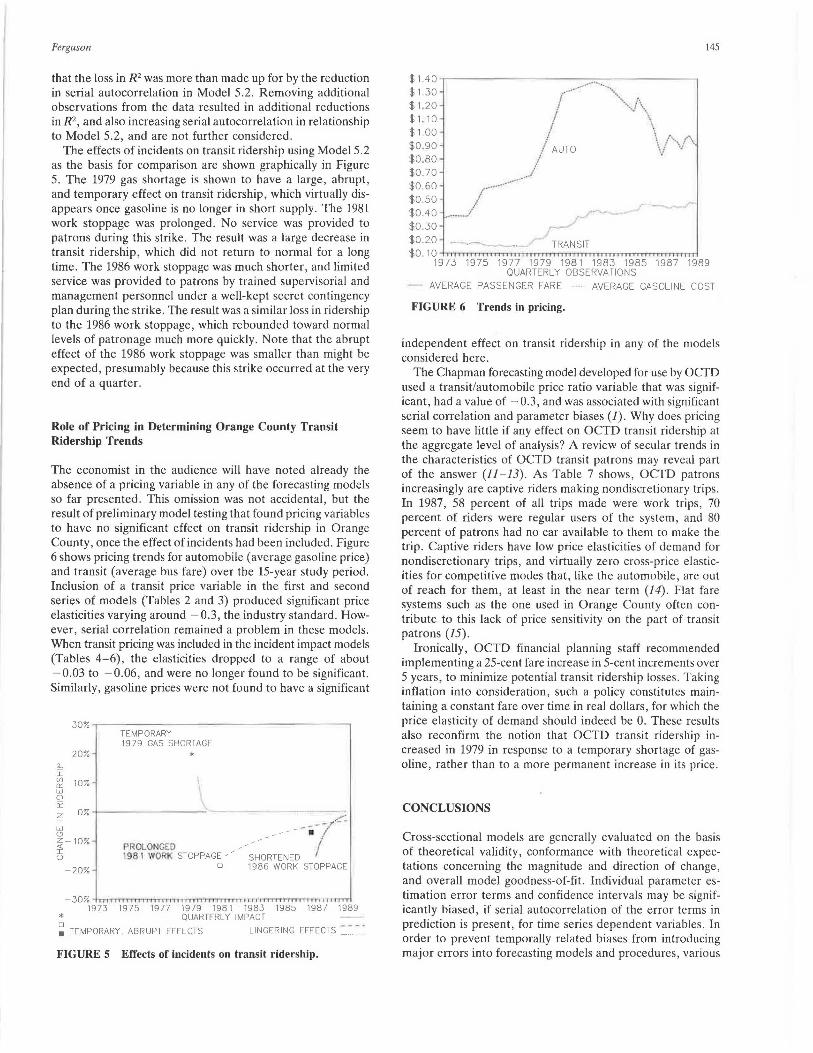
The effects of incidents on transit ridership using Model 5.2 as the basis for comparison are shown graphically in Figure 5. The 1979 gas shortage is shown to have a large, abrupt, and temporary effect on transit ridership, which virtually dis­appears once gasoline is no longer in short supply. The 1981 work stoppage was prolonged. No service was provided to patrons during this strike. The result was a large decrease in transit ridership, which did not return to normal for a long time. The 1986 work stoppage was much shorter, and limited service was provided to patrons by trained supervisorial and management personnel under a well-kept secret contingency plan during the strike. The result was a similar loss in ridership to the 1986 work stoppage, which rebounded toward normal levels of patronage much more quickly. Note that the abrupt effect of the 1986 work stoppage was smaller than might be expected, presumably because this strike occurred at the very end of a quarter.

Role of Pricing in Determining Orange County Transit Ridership Trends

The economist in the audience will have noted already the absence of a pricing variable in any of the forecasting models so far presented . This omission was not accidental, but the result of preliminary model testing that found pricing variables to have no significant effect on transit ridership in Orange County, once the effect of incidents had been included. Figure 6 shows pricing trends for automobile (average gasoline price) and transit (average bus fare) over the 15-year study period. Inclusion of a transit price variable in the first and second series of models (Tables 2 and 3) produced significant price elasticities varying around - 0.3, the industry standard. How­ever, serial correlation remained a problem in these models. When transit pricing was included in the incident impact models (Tables 4-6), the elasticities dropped to a range of about -0.03 to -0.06, and were no longer found to be significant. Similarly, gasoline prices were not found to have a significant

20%

I

~ 10% w 0 ii' ~ w 0 ~ - 103

u -203

TEMPORARY 1979 GAS SHORTAGE

*

-------·1--,re'.. PROLONGED _- -19.81 WORK STOPPAGE - , SHORTENED

o 1986 WORK STOPPAGE

-30% , ii ft jj I iJ I I 11iiIiIf1111tIiiIE111I1 I ii 41 I (I

1973 197 5 1977 1979 1981 1983 1985 1987 1989 * OUARTERL Y IMPACT

~ TEMPORARY, ABRUPT EFFECTS LINGERING EFFECTS ::_ ~.: .. :

FIGURE 5 Effects of incidents on transit ridership.

145

$1.40 ,----------.... -.--..-:::-~-...• -. - ----,

$1.30 -···· ' $1 .20 i ·· .. ·J\ $1 . 10 i \

I \ $1.00 / \/'-,.I\ $0.90 I AUTO \; ., $0 .80 I . $0.70 ; $0.60 ("_ ..• -·-·_.. .. ·

:~:~~ ........ / $0.30

$0.20 TRANSIT $ 0. 10 ..j...,...,....,.....,..M'TTTTTl'°"""ITTTTTTT-n'n"nTl'TTTTTTl'TTTnTTTTTl,.....,l'TTTm

1973 1975 1977 1979 1981 1983 1985 1987 1989 QUARTERLY OBSERVATIONS

AVERAGE PASSENGER FARE ...... AVERAGE GASOLINE COST

FIGURE 6 Trends in pricing.

independent effect on transit ridership in any of the models considered here.

The Chapman forecasting model developed for use by OCTD used a transit/automobile price ratio variable that was signif­icant, had a value of -0.3, and was associated with significant serial correlation and parameter biases (J) . Why does pricing seem to have little if any effect on OCTD transit ridership at the aggregate level of analysis? A review of secular trends in the characteristics of OCTD transit patrons may reveal part of the answer (11-13). As Table 7 shows, OCTD patrons increasingly are captive riders making nondiscretionary trips . In 1987, 58 percent of all trips made were work trips, 70 percent of riders were regular users of the system, and 80 percent of patrons had no car available to them to make the trip . Captive riders have low price elasticities of demand for nondiscretionary trips, and virtually zero cross-price elastic­ities for competitive modes that, like the automobile, are out of reach for them, at least in the near term (14) . Flat fare systems such as the one used in Orange County often con­tribute to this lack of price sensitivity on the part of transit patrons (15) .

Ironically, OCTD financial planning staff recommended implementing a 25-cent fare increase in 5-cent increments over 5 years, to minimize potential transit ridership losses . Taking inflation into consideration, such a policy constitutes main­taining a constant fare over time in real dollars , for which the price elasticity of demand should indeed be 0. These results also reconfirm the notion that OCTD transit ridership in­creased in 1979 in response to a temporary shortage of gas­oline, rather than to a more permanent increase in its price .

CONCLUSIONS

Cross-sectional models are generally evaluated on the basis of theoretical validity, conformance with theoretical expec­tations concerning the magnitude and direction of change, and overall model goodness-of-fit. Individual parameter es­timation error terms and confidence intervals may be signif­icantly biased, if serial autocorrelation of the error terms in prediction is present, for time series dependent variables. In order to prevent temporally related biases from introducing major errors into forecasting models and procedures, various

146 TRANSPORTATION RESEARCH RECORD 1297

TABLE 7 SECULAR TRENDS IN OCTD RIDER CHARACTERISTICS

Year of On-Board Survey OCTD Rider Characteristics 19761 19791 19822 19873

Regular Rider4 52% 63% 70% 70%

Trip Purpose 58%5 Work 35% 46% 46%

School 35% 25% 26% 18% Shopping 10% 11% 10% 7% Recreation 7% 5% 4% 5% Other 13% 13% 14% 12%

Age Under 16 12% 10% 8% 8% 16-64 79% 80% 82% 83% Over 65 9% 10% 10% 9%

Female 58% 58% 57% 54%

Low ~ncome6 74% 55% 51% 45%

No Car Available for Trip 76% 71% 74% 80%

Ethnicity White not not 64% 46% Hispanic asked asked 21% 34% Asian 8% 7% Black 5% 6%

Sample Size not 10,669 21,866 approx. available 17,000

1. DMJM and COMSIS Corp., 1981. 2. TRAM, 1983. 3. NuStats, Inc., 1988. 4. Rides five or more days per week. 5. This figure may be high, in that the 1987 system-wide on-board survey sampled bus trips

in the a.m. only, rather than all day. 6. Annual household income less than $15,000, in cu"ent dollar.r.

tech niques are available. Generally explicit rcpres ntation of the underlying theorelicaJ temporal proce es through tht: use of time series tran formation of the dependent variable , are required to reduce serial autocorrelation, absent the use of indirect estimation methods that are not discussed here. Ostram (4) provides an introduction to indirect estimation techniques, for those who might be interested.

Time series methods include the use of serial and seasonal autoregressive terms, djfferenced or integrated equation , moving average models , etc. If the independent variables u ed in the model are influenced by temporal processes, these should be considered, particularly if such "independent" temporal processes are related to those endogenou temporal proces es that are known or hypothe ized to infiuence the dependent variable.

Models of the type discussed in this paper may provide more reliable mea ures f policy sensitivity, as well as more accurate forecasts of future conditions with respect to the dependent variable. These improvem nts can be tested em­pirically using ex ante or ex post comparative evaluation mea­sures. Ex ante evaluation requires making a foreca t and waiting for the forecast period to expire before comparing foreca t and actual results. Ex post evaluation or backfore­casting, is done by excluding some of the most recently avail­able data from model estimation, and comparing this model

output with actual results. Technically, only information on exogenous variables that was available before the backfore­cast time period should be used in making ex post backfore­casts, for the sake ::if methodological consi tency. The model di cus ed here will probably increase in utility to planners and µulicy analy cs as time series analys1 technique and data become more readily available and understood. Rand m sam­ples of time series data can be used to lower data collection co ts, as long as sucb data are sampled systematically (16,17). The use of uch techniques in research and development eem to be increasing. Periodic updating, t tin , and valuati n of uch time series m del re ults a are in use by pra ticing planners will enhance under tanding and abi lity to use the e versatile methods in the future. Practical advantages of thi class of methods should include more accurate foreca ting abili ty, although this must await further testing of application. in the field for verification.

In terms of policy, the effects of incidents on transit rider­shlp can be modeled quite accurately to determine temporal variations in the lingering effect of such incident . The ability to measure pa t responses to incidents hould hel1 planner and decj ion makers in preparing for anticipated future hocks to transit performance, wheth r po itive or negative in nature. lr would be useful to know if the results reported here for incidents can be duplicated partially or wholly in other parts

Ferguson

of the country, with similar or different types of transit mar­kets in operation. A 1966 transit strike in New York City resulted in permanent regular ridership losses of only 2.1 percent for work trips, 2.6 percent for shopping trips, and 2.4 percent for all other trips, on the basis of an ex post travel behavior survey (18). Are the measured results for Orange County reported here much greater because of differences in sampling procedures, differences in modeling procedures, dif­ferences in the timing of work stoppage occurrence, differ­ences in the spatial configuration of transit markets, or other factors? Additional study using data from multiple transit agencies might assist in answering some of these questions.

ACKNOWLEDGMENTS

The author would like to thank Andrew Weiss of the Uni­versity of Southern California and Larry Hata of OCTD for their assistance. OCTD provided the original data, as well as valuable technical support. The Center for Economic Re­search of Chapman College provided an excellent modeling foundation on which to base this analysis.

REFERENCES

1. E. Ferguson and P. E. Patterson. CR TIME: Simultaneous Time-Series and Cross-Sectional Regrc ion Analysis. In Klos­terman, Richard, Richard Brail & Earl Broussard, eds., Spread­sheet Models for Urban 011d Regional Analysis, Rll!gers Univer­sity, Center for Urban Policy and Research , New Brunswick, N.J., 1991.

2. Center for Economic Research. Orange County Transit District Econometric Forecasting Model . Chapman College, Tustin, Calif., Aug. 19 9.

3. E . Ferguson. U.S. Transit Managcmcni and Performance: Local and National Priorities and the Impact of Technology. Trans­porlation Planning and Technology, Vol. 14, 1989, pp. 199- 215.

4. C. W. Ostrom. Jr. Time Series /\ 110/ysis: Regre.1·sion Techniques. Quantitative Applications in the Social Sciences, Vol. 9, Sage Publications, Beverly Hills, Calif., 1978.

147

5. T. Kina! and J. Ratner. A VAR Forecasting Model of a Regional Economy: Its Con truction and Comparative Accuracy. lnter-11atio11al Regional ScicnctJ Review, Vol. 10, No. 2, 1986, pp. 113-126.

6. J. Durbin and G. S. Watson. Testing for Serial Correlation in Least Squares Regression. Biometrika, Vol. 38, 1951, pp. 159-177.

7. H. Habibagahi and J. L. Pratschke. A omparison of the Power of the von Neumann Ra tio, Durbin-Wat on and Geary Tc ts. Re11iew of Economics am/ tmistics . May 1972, pp. 179- 1 5.

8. J, Durbin . Tc ·Ling for erial Autocorrclntion in Len t- ' qtiares Regression When omc of the Regre · ors are Lagged Dependent Vaiable . Econometrica Vol. 3 , No. 3, 1970, pp. 410- 421.

9. M. Nerlove and K. F. Wallis. Use of the Durbin-Watson Statistic in Inappropriate Situations. Econometrica, Vol. 34, No. 1, 1966, pp. 235 - 238.

10. M. Kyte, J. Stoner, and J. Cryer. A Time-Series Analysis of Public Transit Ridership in Portland, Oregon, 1971-1982. Trans­portation RI! earch A, Vol. 22, No . 5, 1988, pp. 345- 359.

11. Dnniel, Mann, Johnson, & Mendenhall and OM IS orp.1979 OCTD On-Board Survey. Orange County Transit District, Gar­den Grove, Calif., 1981.

12. TRAM. 1982 OCTD On-Board Survey. Orange County Transit District, Garden Grove, Calif., 1983.

13. NuStats, Inc. 1987 OCTD On-Board Survey. Orange County Transit District, Garden Grove, Calif., 1988.

14. A. M . Lago and P. D. Mayw rm. Transit Fare Elasticities by Fare Structure Elements and Ridership Submarkets. Transit Journal , Vol. 7, No. 2, 1981, pp. 5-14.

15. R. Ccrvero. Transit Cro s-Subsidies. Transportation Quarterly. Vol. '.36 No. 3, J982, pp. 377- 389.

16. A. A. Wei · . Systcmalic Sampl ing and T1.:111poral Aggrcgntion in Time eries Models. Jouma/ of Eco110111e1rics. 26:271 - 281 , 1984.

17. H. Lii1ke1 ohl. Forecn ling Vector ARMA Procc es With Sys-1enrn1ic;illy Mi ing Obscrvntions. Juurntil of JJ11slness & Eco­nomic Statistics. Vol. 4, No. 3, L9 6, pp. 375- 390.

18. Barrington & C mpany. The £}feet of tile 1966 ew York ity Transit Strike on tile Travel Behavior of Regular User , New York City Transit Authority, New York, 1967.

The author is solely responsible for any errors or omissions remaining in this paper.

Publication of this paper sponsored by Committee on Public Trans­portation Planning and Development.