TEMPORAL CORRELATION OF DEFAULTS IN SUBPRIME SECURITIZATION

ERIC HILLEBRAND, AMBAR N. SENGUPTA, AND JUNYUE XU

ABSTRACT. The securitization of subprime mortgages in instruments like mortgage-backedsecurities and collateralized debt obligations is one of the key ingredients to the current finan-cial crisis. During 2007 and 2008, subprime defaults increased sharply, displaying high serialcorrelation in their arrival. Subprime default events depend on house price changes. We estab-lish a link between the dynamics of house price changes and the dynamics of default rates inthe Gaussian copula framework by specifying a time series model for a common risk factor.We show analytically and in simulations that serial correlation propagates from the commonrisk factor to default rates. We simulate prices of mortgage-backed securities, which are secu-ritized from pools of mortgages using a waterfall structure. We find that subsequent vintagesof these securities inherit temporal correlation from the common risk factor. The findings inthis paper formalize one important dynamic of the subprime crisis: transmission of the declinein housing prices after 2006 into financial derivatives based on subprime mortgages.KEYWORDS: subprime mortgage, housing prices, mortgage-backed securities, collateralizeddebt obligations, financial crisis, vintage correlation, serial correlation, time series model,Gaussian copulaJEL Codes: C02, E44, G01, G13, G21

1. INTRODUCTION

From its beginning in the summer of 2007, the subprime crisis has plunged the world intoone of the worst recessions in history. At the center of the crisis is the subprime mortgagemarket, where lenders provide mortgages to borrowers with poor credit standing. During thecrisis, subprime mortgages created at different times have defaulted one after another. Thedefault arrivals of these mortgages were serially correlated. Figure 1, lower panel, shows thetime series of serious delinquency rates of subprime mortgages from 2002 to 2009.1 This seriesobviously displays very high serial correlation. Defaults of subprime mortgages are closelyconnected to house price fluctuations, as suggested, among others, by Gorton (2008).2 Most

Date: October 21, 2010.1By definition of the Mortgage Banker Association, seriously delinquent mortgages refer to mortgages that haveeither been delinquent for more than 90 days or are in the process of foreclosure.2For example, see also Bajari, Chu, and Park (2008), Daglish (2009), Hayre, Saraf, Young, and Chen (2008).

1

2 E. HILLEBRAND, A. SENGUPTA, AND J. XU

subprime mortgages are Adjustable-Rate Mortgages (ARM). This means that the interest rateon a subprime mortgage is fixed at a relatively low level for a “teaser” period, usually two tothree years, after which it increases substantially. Gorton (2008) points out that the interestrate usually resets to such a high level that it “essentially forces” a mortgage borrower torefinance or default after the teaser period. Therefore, whether the mortgage defaults or not islargely determined by the borrower’s access to refinancing. At the end of the teaser period, ifthe value of the house is much greater than the outstanding principal of the loan, the borroweris likely to be approved for a new loan since the house serves as collateral. On the other hand,if the value of the house is less than the outstanding principal of the loan, the borrower isunlikely to be able to refinance and has to default.

Gorton’s view is supported by data. Figure 1 displays two-year changes in the Case-Shillerindex (upper panel) and subprime ARM serious delinquency rates (lower panel) using quar-terly data from 2002 to 2009. It is clear that from 2002 to 2006, subprime delinquency ratesdeclined as home prices climbed steadily. The delinquency series reached its trough aroundthe same time the home price peaked. When the house price index started to drop in 2006,delinquency rates began to increase significantly, which triggered the subprime crisis.

Therefore, the hypothesis that this paper examines is that the dynamics of defaults are inher-ited from the dynamics of house prices. The aim of this paper is to formalize this relationshipusing the industry-standard framework of a Gaussian copula, which was routinely used toprice derivatives constructed from subprime mortgages. To this end, we introduce the notionof vintage correlation, which captures the correlation of default rates in mortgage pools is-sued at different times. Under certain assumptions, vintage correlation is the same as serialcorrelation. After showing that changes in a housing index can be regarded as a commonrisk factor of individual subprime mortgages, we specify a time series model for the commonrisk factor in the Gaussian copula framework. We show analytically and in simulations thatthe serial correlation of the common risk factor introduces vintage correlation into defaultrates of pools of subprime mortgages of subsequent vintages. In this sense, serial correlationpropagates from the common risk factor to default rates. In simulations of the price behaviorof Mortgage-Backed Securities (MBS) over different cohorts, we find that the price of MBSalso exhibits vintage correlation, which is inherited from the common risk factor of individualmortgages.

TEMPORAL CORRELATION OF DEFAULTS IN SUBPRIME SECURITIZATION 3

The main point of this paper is to provide a formal examination of one of the importantcauses of the current crisis.3 The crisis is understood as a pronounced deviation of the commonrisk factor from its unconditional mean, induced by its serial correlation, and the consequencesfor the instruments that depend on this factor.

Vintage correlation in default rates and MBS prices also has implications for asset pric-ing. To price some derivatives, for example forward starting Collateralized Debt Obligations(CDO), it is necessary to predict default rates of credit assets created at some future time.Knowing the serial correlation of default probabilities can improve the quality of prediction.For risk management in general, some credit asset portfolios may consist of credit derivativesof different cohorts. Vintage correlation of credit asset performance affects these portfolios’risks. For instance, suppose there is a portfolio consisting of two subsequent vintages of thesame MBS. If the vintage correlation of the MBS price is close to one, for example, the payoffof the portfolio has a variance almost twice as big as if there were no vintage correlation.

The outline of the paper is as follows. In Section 2, we introduce the concept of vintagecorrelation and give some examples to provide intuition. We then briefly describe the Gaussiancopula model. We show that changes in a house price index can be seen as a common riskfactor in the copula framework. Section 3 contains the main analytical results. It shows thelink between the serial correlation of the common risk factor and vintage correlation in defaultrates. Section 4 explores this link in two sets of simulations: First, a series of mortgagepools is simulated to illustrate our analytical results. Second, a waterfall structure is simulatedto study the propagation of serial correlation in MBS. In Section 5 we summarize the mainconclusions.

2. MODELING TEMPORAL CORRELATION IN SUBPRIME SECURITIZATION

In this section, we introduce the concept of vintage correlation and give some examples toprovide intuition. We outline the Gaussian copula model. We show that changes in a houseprice index can be seen as a common risk factor in the copula framework.

DEFINITION 1 (Vintage Correlation). Suppose we have a pool of mortgages created at each

time v = 1, 2, · · · , V . Denote the default rates of each vintage observed at a fixed time

3For different perspectives on the causes and effects of the subprime crisis, see also Caballero and Krishnamurthy(2009), Crouhy, Jarrow, and Turnbull (2008), Figlewski (2009), Gorton (2009), Murphy (2008), Reinhart andRogoff (2008), and Reinhart and Rogoff (2009).

4 E. HILLEBRAND, A. SENGUPTA, AND J. XU

T > V as p1, p2, · · · , pV , respectively. We define vintage correlation φj := Corr(p1, pj) for

j = 2, 3, · · · , V as the default correlation between the j − th vintage and the first vintage.

As an example of vintage correlation, consider wines of different vintages. Suppose thereare several wine producers that have produced wines of ten vintages from 2011 to 2020. Thewines are packaged according to vintages and producers, that is, one box contains one vintageby one producer. In the year 2022, all boxes are opened and the percentage of wines that havegone bad is obtained for each box. Consider the correlation of fractions of bad wines betweenthe first vintage and subsequent vintages. This correlation is what we call vintage correlation.

The definition of vintage correlation can be extended easily to the case where the base vin-tage is not the first vintage but any one of the other vintages. Obviously, vintage correlation isvery similar to serial correlation. There are two main differences. First, the consideration is ata specific time in the future. Second, in calculating the correlation between any two vintages,the expected values are averages over the cross-section. That is, in the wine example, expectedvalues are averages over producers. In mortgage pools, they are averages over different mort-gage pools. Only if we assume the same stochastic structure for the cross-section and for thetime series of default rates, vintage correlation and serial correlation are equivalent. We do nothave to make this assumption to obtain our main results. Making this assumption, however,does not invalidate any of the results either. Therefore, we use the terms “vintage correlation”and “serial correlation” interchangeably in our paper.

To model vintage correlation in subprime securitization, we resort to the copula approach.The Gaussian copula approach is widely used in industry to model default correlation acrossnames. A copula is a function that takes the marginal distribution functions of a set of variablesas arguments and returns the joint distribution of the variables. Thus, the copula approachprovides a general way to link univariate marginal distribution functions to their multivariatedistribution function. This feature makes it very useful for modeling multivariate correlations.Frees and Valdez (1998) explain in detail how to specify a copula, and how to simulate amultivariate distribution once its copula form is known.

The credit industry standard copula model was introduced by Li (2000) and is called default-time (or survival-time) Gaussian copula. This model is applicable to all types of CDO, MBS,and almost all other credit derivatives that are derived from multiple assets with credit risk.The idea behind Li’s model is that each credit asset has a default time (or survival time), afterwhich the mortgage defaults. Instead of modeling the correlation between default events ofmortgages, Li proposes a copula approach to capture the joint distribution of default times.

TEMPORAL CORRELATION OF DEFAULTS IN SUBPRIME SECURITIZATION 5

A copula in this case takes the marginal distribution of default times and returns their jointdistribution.

The literature on credit risk pricing with copulas and other models has grown substantiallyin recent years and an exhaustive review is beyond the scope of his paper. Bluhm, Overbeck,and Wagner (2002), Schonbucher (2003), Duffie and Singleton (2003), and Lando (2004)are standard monographs. Some modifications of the standard Gaussian copula model arediscussed. For example, Servigny and Renault (2002) and Das, Freed, Geng, and Kapadia(2006) provide empirical evidence that asset correlation may be stochastic. Andersen andSidenius (2005), Hull, Predescu, and White (2009), and Berd, Engle, and Voronov (2007)allow default correlation to vary over time. Copula models using distribution functions otherthan Gaussians have also been suggested. For example, Andersen, Sidenius, and Basu (2003)and Frey and McNeil (2003) consider the student t-copula. Schonbucher and Schubert (2001)and Laurent and Gregory (2005) discuss the Clayton copula. The Marshall-Olkin copula hasbeen considered by Lindskog and McNeil (2003) and Giesecke (2003). A recent study byBeare (2010) explicitly addresses the temporal correlation problem in copulas.

There are approaches to model default correlation other than default-time copulas. Onemethod relies on the so-called structural model, which goes back to Merton’s (1974) work onpricing corporate debt. An essential point of the structural model is that it links the defaultevent to some observable economic variables. Hull and White (2001) extend the model to amulti-issuer scenario, which can be applied to price corporate debt CDO. It is assumed thata firm defaults if its credit index hits a certain barrier. Therefore, correlation between creditindices determines the correlation of default events. The advantage of a structural model isthat it gives economic meaning to underlying variables. Other approaches to CDO pricing arefound, for example, in Graziano and Rogers (2009) and in Sidenius, Piterbarg, and Andersen(2008). Burtschell, Gregory, and Laurent (2009) provide a comparison of common CDOpricing models.

In this paper, we adopt Li’s (2000) default time copula approach and extend it by adding atime series model for a common risk factor. Each mortgage i of vintage v has a default timeτv,i, which is a random variable representing the time at which the mortgage defaults. If themortgage never defaults, this value is infinity. If we assume that the distribution of τv,i is thesame across all mortgages of vintage v, we have

Fv(s) = P[τv,i < s], ∀i = 1, 2, ..., N, (1)

6 E. HILLEBRAND, A. SENGUPTA, AND J. XU

where the index i denotes individual mortgages and the index v denotes vintages. We assumethat Fv is continuous and strictly increasing. Given this information, for each vintage v theGaussian copula approach provides a way to obtain the joint distribution of the τv,i across i.Generally, a copula is a joint distribution function

C (u1, u2, ..., uN) = P (U1 ≤ u1, U2 ≤ u2, ..., UN ≤ uN) ,

where u1, u2, ..., uN are N uniformly distributed random variables that may be correlated. Itcan be easily verified that the function

C [F1(x1), F2(x2), ..., FN(xN)] = G(x1, x2, ..., xN) (2)

is a multivariate distribution function with marginal distribution functions F1(x1), F2(x2), ...,

FN(xN). Sklar (1959) proved the converse. He showed that for an arbitrary multivari-ate distribution function G(x1, x2, ..., xN) with continuous marginal distributions functionsF1(x1), F2(x2), ..., FN(xN), there exists a unique C such that equation (2) holds. Therefore,in the case of default times, there is a Cv for each vintage v such that

Cv [Fv(τv,1), Fv(τv,2), ..., Fv(τv,N)] = Gv(τv,1, τv,2, ..., τv,N). (3)

The joint distribution function Gv on the right-hand side of equation (3) is the object we wantto obtain. Since we assume Fv to be continuous and strictly increasing, we can find a standardGaussian random variable Xv,i such that

Φ(Xv,i) = Fv(τv,i) ∀v = 1, 2, ..., V ; i = 1, 2, ..., N, (4)

or equivalently,

τv,i = F−1v (Φ(Xv,i)) ∀v = 1, 2, ..., V ; i = 1, 2, ..., N, (5)

where Φ is the standard normal distribution function. To see that this is correct, observe that

P[τv,i ≤ s] = P [Φ(Xv,i) ≤ Fv(s)]

= P[Xv,i ≤ Φ−1 (Fv(s))

]= Φ

[Φ−1 (Fv(s))

]= Fv(s).

Substituting equation (4) into the left-hand side of equation (3), we have

Cv [Φ(Xv,1),Φ(Xv,2), ...,Φ(Xv,N)] = Gv(τv,1, τv,2, ..., τv,N). (6)

TEMPORAL CORRELATION OF DEFAULTS IN SUBPRIME SECURITIZATION 7

Since Φ(·) is the marginal distribution function for all Xv,i, the left-hand side of equation (6)is equal to the joint distribution of Xv,i. The Gaussian copula approach assumes that this jointdistribution has a multivariate normal distribution function ΦN ,

Gv(τv,1, τv,2, ..., τv,N) = ΦN (Xv,1, Xv,2, ..., Xv,N) . (7)

Thus the joint distribution function of default times τv,i is obtained once the correlation matrixof theXv,i is known. A standard simplification in practice is to assume that the pairwise corre-lations between different Xv,i are the same across i. Suppose that the value of this correlationis ρv for each vintage v. Consider the following definition

Xv,i :=√ρvZv +

√1− ρvεi ∀i = 1, 2, . . . , N ; v = 1, 2, . . . , V, (8)

where εv,i are i.i.d. standard Gaussian random variables and Zv is a Gaussian random variableindependent of the εv,i. It can be shown easily that in each vintage v, the variablesXv,i definedin this way have the exact joint distribution function ΦN .

Using the information above, for each vintage v, the Gaussian copula approach obtains thejoint distribution function Gv for default times as follows. First, N Gaussian random variablesXv,i are generated according to equation (8). Second, from equation (5) a set of N defaulttimes τv,i is obtained, which has the desired joint distribution function Gv. In equation (8),the common factor Zv can be viewed as a latent variable that captures the default risk inthe economy, and εi is the idiosyncratic risk for each mortgage. The variable Xv,i can beviewed as a state variable for each mortgage. The parameter ρv is the correlation betweenany two individual state variables. It is obvious that the higher the value of ρv, the greater thecorrelation between the default times of different mortgages.

In pricing derivatives created on subprime mortgages, Monte Carlo simulations are em-ployed to study the default behavior of mortgages by the method described above. In eachsimulation, the default times for all mortgages are generated with the joint distribution Gv.Mortgage i is said to default before time T , if its simulated default time τv,i is less than T . Thevalue of ρv can then be calibrated to market data. The market-implied ρv may vary over time.Indeed, this is supported by empirical evidence provided by Servigny and Renault (2002) andDas, Freed, Geng, and Kapadia (2006). This time dependence may capture dynamic cor-relation between default events not explicitly captured in the default time copula approach.One way to explicitly model the dynamics of defaults is to specify a stochastic process fordefault correlation. This approach is called stochastic correlation (see for example Andersen

8 E. HILLEBRAND, A. SENGUPTA, AND J. XU

and Sidenius (2005) and Hull, Predescu, and White (2009)). Das, Freed, Geng, and Kapadia(2006) propose a model where the default intensity is determined by the state of the economy,which follows a Markov process.

In this paper, we propose a time series model for the common risk factor Zv in the copulaframework and show that its serial correlation propagates to the default rates. To illustratethe intuition behind our approach, we first give a structural interpretation for the common riskfactor Zv of subprime ARM.

Assume that we have a pool of N mortgages i = 1, . . . , N for each vintage v = 1, . . . , V .Each individual mortgage within a pool has the same initiation date v and interest adjustmentdate v′ > v. Let Yv,i be the change in the logarithm of the price Pv,i of borrower i’s (of vintagev) house during the teaser period [v, v′]. Consider

Yv,i := logPv′,i − logPv,i = Hv + ev,i, (9)

where Hv := log Iv′ − log Iv is the change in the logarithm of a housing market index Iv, andev,i are i.i.d. normal random variables for all i = 1, 2, ..., N , and v = 1, 2, ..., V . As outlinedin the introduction, default rates of subprime ARM depend on house price changes during theteaser period. If the house price fails to increase substantially or even declines, the mortgageborrower cannot refinance, absent other substantial improvements in income or asset position.They have to default shortly after the interest rate is reset to a high level. We assume that thedefault, if it happens, occurs at time v′. Therefore, we assume that a mortgage defaults if andonly if Yv,i < Y ∗, where Y ∗ is a predetermined threshold. For example, if we set Y ∗ = 0,we are implicitly assuming that if the house price increases, the mortgage borrower is able torefinance. Otherwise, they cannot be approved for a new loan and have to default. Supposewe have a portfolio of N mortgages, which satisfy the assumptions above. Now, if we assumea form of stationary stochastic process for Hv, say an ARMA(p,q) process, we can simulatethe default rates over time in the portfolio by Monte Carlo simulation.

We can now give a structural interpretation of the common risk factor Zv in the Gaussiancopula framework. Define

Z ′v :=Hv

σH, (10)

where σH is the unconditional standard deviation of Hv. Then we have

Yv,i = Z ′vσH + ev,i.

TEMPORAL CORRELATION OF DEFAULTS IN SUBPRIME SECURITIZATION 9

Further standardizing Yv,i, we have

X ′v,i :=Yv,iσY

=Z ′vσH + ev,i

σY

=σH√σ2H + σ2

e

Z ′v +σe√

σ2H + σ2

e

ε′v,i

where σe is the standard deviation of ev,i, and ε′v,i := ev,i/σe. The third equality follows fromthe fact that

σY =√σ2H + σ2

e .

Define

ρ′ :=σ2H

σ2H + σ2

e

.

ThenX ′v,i =

√ρ′Z ′v +

√1− ρ′ε′v,i ∀i = 1, 2, . . . , N ; t = 1, 2, . . . , T (11)

Note that equation (11) has exactly the same form as equation (8). The default event is definedas X ′v,i < X∗′ where

X∗′ :=Y ∗√σ2H + σ2

e

.

Letτ ′v,i := F−1v

(Φ(X ′v,i)

),

andτ ∗′v := F−1v (Φ(X∗′)) ,

then the default event can be defined equivalently as τ ′v,i ≤ τ ∗′. The comparison betweenequation (11) and (8) shows that the common risk factor Zv in the Gaussian copula model forsubprime mortgages can be interpreted as a standardized change in a house price index. Ofcourse, the interpretation of house prices depending on an index is but one possible viewpoint.The same argument could be applied, for example, to credit card debt that depends on the stateof the economy, which could be proxied by changes in gross domestic product.

In light of this structural interpretation, the common risk factor Zv is very likely to beserially correlated across subsequent vintages. In the example above, Z ′v is proportional to amoving average of monthly log changes in a housing price index. To see this, let v be the time

10 E. HILLEBRAND, A. SENGUPTA, AND J. XU

of origination and v′ be the end of the teaser period. Then,

Hv =

∫ v′

v

d log Iτ ,

where I is the house price index. For example, if we measure house price index changesquarterly, as in the case of the Case-Shiller housing index, we have

Hv =∑

τ∈[v,v′]

(log Iτ − log Iτ−1), (12)

where the unit of τ is a quarter. If we model this index by some random shock arriving eachquarter, equation (12) is a moving average process. Therefore, from equation (10) we knowthat Z ′v has positive serial correlation. That is, even though the stationary distribution of Zremains constant, the process can undergo long excursions away from the unconditional mean,depending on the degree of serial correlation. Figure 1 shows that in the case of the housingindex, this serial correlation is very pronounced. A pronounced excursion of the common riskfactor below the unconditional mean and its ramifications for the dependent instruments areour understanding of a crisis in this paper.

3. MAIN THEOREMS - VINTAGE CORRELATION IN DEFAULT RATES

Since the common risk factor is likely to be serially correlated, we examine the implicationsfor the stochastic properties of mortgage default rates. Most subprime ARM have a teaserperiod of two years, therefore equation (12) suggests that a two-year house index change canbe used as a common risk factor for these mortgages. Figure 1 compares two-year changes inthe Case-Shiller index with subprime ARM serious delinquency rates. The two variables arehighly and negatively correlated with each other. To study this observation analytically, wespecify a time series model for the common risk factor in the Gaussian copula approach. Wethen determine the relationship between the serial correlation of the default rates and that ofthe common risk factor.

PROPOSITION 1 (Default Probabilities and Numbers of Defaults). Let k = 1, 2, ..., N ,

Xk =√ρZ +

√1− ρ εk, and X ′k =

√ρ′Z ′ +

√1− ρ′ ε′k (13)

with

Z ′ = φZ +√

1− φ2 u, (14)

TEMPORAL CORRELATION OF DEFAULTS IN SUBPRIME SECURITIZATION 11

where ρ, ρ′ ∈ (0, 1), φ ∈ (−1, 1), and Z, ε1, ..., εN , ε′1, ..., ε′N , u are mutually independent

standard Gaussians. Consider next the number of Xk that fall below some threshold X∗, and

the number of X ′k below X ′∗:

A =N∑k=1

1{Xk≤X∗}, and A′ =N∑k=1

1{X′k≤X′∗}, (15)

where X∗ and X ′∗ are constants. Then

Cov(A,A′) = N2 Cov(p, p′), (16)

where

p = p(Z) := P[Xk ≤ X∗ |Z] = Φ

(X∗ −

√ρZ

√1− ρ

), and p′ = P[X ′k ≤ X ′∗ |Z ′] = p′(Z ′).

(17)Moreover, the correlation between A and A′ equals the correlation between p and p′, in the

limit as N →∞.

Proof. We first show that

E[AA′] = E [E[A |Z]E[A′ |Z ′]] . (18)

Note that A is a function of Z and ε = (ε1, . . . , εN), and A′ is a function (indeed, the samefunction as it happens) of Z ′ and ε′ = (ε′1, . . . , ε

′N). Now for any non-negative bounded Borel

functions f and g onRN , and any non-negative bounded Borel functions F andG onR×RN ,we have, on using self-evident notation,

E[f(Z)g(Z ′)F (Z, ε)G(Z ′, ε′)]

=

∫f(z)g(φz +

√1− φ2x︸ ︷︷ ︸z′

)F (z, y1, ..., yN)G(z′, y′1, ..., y′N) dΦ(z, x,y,y′)

=

∫f(z)g(z′)

[{∫F (z, y1, ..., yN) dΦ(y)

}{∫G(z′, y′1, ..., y

′N) dΦ(y′)

}]dΦ(z, x)

= E [f(Z)g(Z ′)E[F (Z, ε) |Z]E[G(Z ′, ε′) |Z ′]] .(19)

This says that

E [F (Z, ε)G(Z ′, ε′) |Z,Z ′] = E[F (Z, ε) |Z]E[G(Z ′, ε′) |Z ′]. (20)

12 E. HILLEBRAND, A. SENGUPTA, AND J. XU

Taking expectation on both sides of equation (20) with respect to Z and Z ′, we obtain

E [F (Z, ε)G(Z ′, ε′)] = E [E[F (Z, ε) |Z]E[G(Z ′, ε′) |Z ′]] . (21)

Substituting F (Z, ε) = A, and G(Z ′, ε′) = A′, we have equation (18) and

E[AA′] = E [E[A |Z]E[A′ |Z ′]]

= E[NpNp′] = N2E[pp′],(22)

The last line is due to the fact that conditional on Z, A is a sum of N independent indicatorvariables and follows a binomial distribution with parameters N and Ep. Applying (21) againwith F (Z, ε) = A, andG(Z ′, ε′) = 1, or indeed, much more directly by repeated expectations,we have

E[A] = NE[p], and E[A′] = NE[p′]. (23)

Hence we conclude that

Cov(A,A′) = E(AA′)− E[A]E[A′]

= N2E[pp′]−N2E[p]E[p′]

= N2 Cov(p, p′).

We have

Var(A) = E[E[A2 |Z]

]−N2(E[p])2

= E[Np+N(N − 1)p2]−N2(E[p])2

= NE[p(1− p)] +N2 Var(p).

(24)

Similarly,Var(A′) = NE[p′(1− p′)] +N2 Var(p′).

Putting everything together, we have for the correlations:

Corr(A,A′) =N2 Cov(p, p′)√

NE[p(1− p)] +N2 Var(p)√NE[p′(1− p′)] +N2 Var(p′)

=Corr(p, p′)√

1 + E[p(1−p)]N Var(p′)

√1 + E[p′(1−p′)]

N Var(p)

= Corr(p, p′) as N →∞.

(25)

�

TEMPORAL CORRELATION OF DEFAULTS IN SUBPRIME SECURITIZATION 13

THEOREM 1 (Vintage Correlation in Default Rates). Consider a pool ofN mortgages created

at each time v, where N is fixed. Suppose within each vintage v, defaults are governed by a

Gaussian copula model as in equations (1), (5), (7), and (8) with common risk factor Zvbeing a zero-mean stationary Gaussian process. Assume further that ρv = Corr(Xv,i, Xv,j),

the correlation parameter for state variables Xv,i of individual mortgages of vintage v, is

positive. Then, Av and Av′ , the numbers of defaults observed at time T within mortgage

vintages v and v′ are correlated if and only if φv,v′ = Corr(Zv, Zv′) 6= 0, where Zv is the

common Gaussian risk factor process. Moreover, in the large portfolio limit, Corr(Av, Av′)

approaches a limiting value determined by φv,v′ , ρv, and ρv′ .

Proof. Conditional on the common risk factor Zv, the number of defaults Av is a sum of Nindependent indicator variables and follows a binomial distribution. More specifically,

P(Av = k|Zv) =

(N

k

)pkv(1− pv)N−k (26)

where pv is the default probability conditional on Zv, i.e.,

pv = P(τv,i ≤ τ ∗|Zv) = P(Xv,i ≤ X∗v |Zv),

withX∗v = Φ−1(Fv(T )),

where Fv(T ) is the probability of default before the time T . Then

pv = P (Xv,i ≤ X∗v |Zv)

= P

(εi ≤

X∗v −√ρtZv√

1− ρv

)

=1√2π

∫ X∗v−√ρtZv√

1−ρv

−∞exp

(−x

2

2

)dx

= Φ (Z∗v ) ,

(27)

where

Z∗v =X∗v −

√ρvZv√

1− ρv. (28)

Similarly,pv′ = Φ (Z∗v′) , (29)

where

Z∗v′ =X∗v′ −

√ρv′Zv′√

1− ρv′. (30)

14 E. HILLEBRAND, A. SENGUPTA, AND J. XU

Note that if Zv and Zv′ are jointly Gaussian with correlation coefficient φv,v′ , we can write

Zv = φv,v′Zv′ +√

1− φ2v,v′ uv,v′ for t > j, (31)

where uv,v′ are standard Gaussians that are independent of Zv′ . Combining equation (28), (30)and (31), we have

Z∗v = aφv,v′Z∗v′ +

X∗t − bφjX∗v′√1− ρt

−

√ρv(1− φ2

v,v′)√

1− ρvuv,v′ , (32)

where

a =

√ρv(1− ρv′)ρv′(1− ρv)

, b =

√ρvρv′.

Therefore,

Cov(pv, pv′) = Cov (Φ(Z∗v ),Φ(Z∗v′))

= Cov

Φ

aφv,v′Z∗v′ + X∗v − bφv,v′X∗v′√1− ρv

−

√ρv(1− φ2

v,v′)√

1− ρvuv,v′

,Φ (Z∗v′)

.

(33)

Since a > 0 as ρv ∈ (0, 1), we know that the covariance and the correlation between pv andpv′ are determined by φv,v′ , ρv, and ρv′ . They are nonzero if and only if φv,v′ 6= 0. ApplyingProposition 1, we know that

Corr(Av, Av′) =Corr(pv, pv′)√

1 + E[pv(1−pv)]N Var(pv′ )

√1 +

E[pv′ (1−pv′ )]N Var(pv)

∀v 6= v′. (34)

Therefore, Av and Av′ have nonzero correlation as long as pv and pv′ do. �

Equations (33) and (34) provide closed-form expressions for the serial correlation of defaultrates pv of different vintages and the number of defaults Av. However, we cannot directlyread from equation (33) how the vintage correlation of default rates depends on the serialcorrelation parameter φv,v′ in the common risk factor. The theorem below shows that thisdependence is always positive.

THEOREM 2 (Dependence on Common Risk Factor). Under the same settings as in Theorem

1, assume that both the serial correlation φv,v′ of the common risk factor and the individual

state variable correlation ρv are always positive. Then the number Av of defaults in the

vintage-v cohort by time T is positively correlated with the number Av′ in the vintage-(v′)

TEMPORAL CORRELATION OF DEFAULTS IN SUBPRIME SECURITIZATION 15

cohort. Moreover, this correlation is an increasing function of the serial correlation parameter

φv,v′ in the common risk factor.

Proof. We will use the notation established in Proposition 1. We can assume that v 6= v′.Recall that in the Gaussian copula model, name i in the vintage-v cohort defaults by time Tif the standard Gaussian variable Xv,i falls below a threshold X∗v . The unconditional defaultprobability is

P[Xv,i ≤ X∗v ] = Φ(X∗v ).

For the covariance, we have

Cov(Av, Av′) =N∑

k,l=1

Cov(1[Xv,k≤X∗v ],1[Xv′,l≤X∗v′ ])

= N2Cov(1[X≤X∗v ],1[X′≤X∗v′ ]),

(35)

where X,X ′ are jointly Gaussian, each standard Gaussian, with mean zero and covariance

E[XX ′] = E[Xv,kXv′,l],

which is the same for all pairs k, l, since v 6= v′. This common value of the covariance arisesfrom the covariance between Zv and Zv′ along with the covariance between any Xv,k with Zv;it is

Cov(X,X ′) = φj√ρvρv′ . (36)

Now since X,X ′ are jointly Gaussian, we can express them in terms of two independentstandard Gaussians:

W1 := X,

W2 :=1√

1− ρvρv′φ2v,v′

[X ′ − φv,v′√ρvρv′X]. (37)

We can check readily that these are standard Gaussians with zero covariance, and

X = W1,

X ′ = φv,v′√ρvρv′W1 +

√1− ρvρv′φ2

v,v′W2.(38)

Letα = φv,v′

√ρvρv′ .

16 E. HILLEBRAND, A. SENGUPTA, AND J. XU

The assumption that ρ and φv,v′ are positive (and, of course, less than 1) implies that

0 < α < 1.

Note that the covariance between pv and pv′ can be expressed as

Cov(pv, pv′) = E(pvpv′)− E(pv)E(pv′)

= E[E[1{Xv,i≤X∗v}

∣∣Zv]E [1{Xv′,i≤X∗v′}∣∣∣Zv′]]− E(pv)E(pv′)

= E[1{Xv,i≤X∗v}1{Xv′,i≤X∗v′}

]− E(pv)E(pv′)

= P [Xv,i ≤ X∗v , Xv′,i ≤ X∗v ]− E(pv)E(pv′)

= P[W1 ≤ X∗v , αW1 +

√1− α2W2 ≤ X∗v′

]− E(pv)E(pv′)

=

∫ X∗v

−∞Φ

(X∗v′ − αw1√

1− α2

)ϕ(w1) dw1 − E(pv)E(pv′),

where ϕ(·) is the probability density function of the standard normal distribution. The thirdequality follows from equation (21). The fifth equality follows from equation (38). The un-conditional expectation of pv is independent of α, because

E(pv) = E (P(Xv,i ≤ X∗v |Zv))

= P(Xv,i ≤ X∗v )

= Φ(X∗v ).

(39)

It follows that

∂

∂αCov(pv, pv′) =

∫ X∗v

−∞ϕ

(X∗v′ − αw1√

1− α2

)ϕ(w1)

∂(X∗v′−αw1√1−α2

)∂α

dw1

=

∫ X∗v

−∞ϕ

(X∗v′ − αw1√

1− α2

)ϕ(w1)

−w1 + αX∗v′

(1− α2)32

dw1

= − 1

(1− α2)32

∫ X∗v

−∞(w1 − αX∗v′)ϕ

(X∗v′ − αw1√

1− α2

)ϕ(w1) dw1.

(40)

TEMPORAL CORRELATION OF DEFAULTS IN SUBPRIME SECURITIZATION 17

The last two terms in the integrand can be rewritten as

ϕ

(X∗v′ − αw1√

1− α2

)ϕ(w1) =

1

2πexp

[−(X∗v′ − αw1)

2

2(1− α2)− w2

1

2

]=

1

2πexp

[−X

∗v′2 − 2αX∗v′w1 + w2

1α2 + w2

1(1− α2)

2(1− α2)

]=

1

2πexp

[−w

21 − 2αX∗v′w1 + α2X∗v′

2 +X∗v′2(1− α2)

2(1− α2)

]=

1

2πexp

[−(w1 − αX∗v′)

2 +X∗v′2(1− α2)

2(1− α2)

].

(41)

Substituting equation (41) into (40), we have

∂

∂αCov(pv, pv′) = −

exp(−X∗

v′2

2

)2π (1− α2)

32

∫ X∗v

−∞(w1 − αX∗v′) exp

[−(w1 − αX∗v′)

2

2(1− α2)

]dw1.

Make a change of variable and let

y :=w1 − αX∗v′√

1− α2.

It follows that

∂

∂αCov(pv, pv′) = −

exp(−X∗

v′2

2

)2π√

1− α2

∫ X∗v−αX∗v′√

1−α2

−∞y exp

(−y

2

2

)dy

=exp

(−X∗

v′2

2

)2π√

1− α2exp

[−(X∗v − αX∗v′)

2

2(1− α2)

]

=1

2π√

1− α2exp

(−X

∗v2 − 2αX∗vX

∗v′ +X∗v′

2

2(1− α2)

)> 0.

Thus, we have shown that the partial derivative of the covariance with respect to α is positive.Since

α =√ρvρv′φv,v′ ,

with ρs and φv,v′ assumed to be positive, we know that the partial derivatives of the covariancewith respect to φv,v′ , ρv and ρv′ are also positive everywhere. Note that the unconditionalvariance of pv is independent of φv,v′ (although dependent of ρs), which can be seen fromequation (27). It follows that the serial correlation of pv has positive partial derivative withrespect to φv,v′ . Recall equation (33), which shows that the covariance of pv and pv′ is zero forany value of ρs when φv,v′ = 0. This result together with the positive partial derivatives of the

18 E. HILLEBRAND, A. SENGUPTA, AND J. XU

covariance with respect to φv,v′ ensure that the covariance and thus the vintage correlation ofpv and pv′ is always positive. From equation (34), noticing the fact that both the expectationand variance of pv are independent of φv,v′ , we know that the correlation between Av and Av′

must also be positive everywhere and monotonically increasing in φv,v′ . �

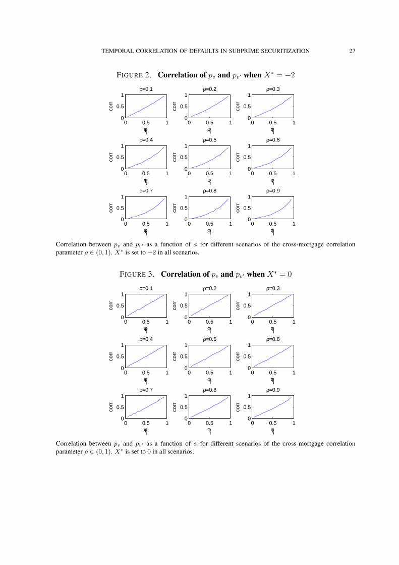
So far we have shown that the vintage correlation of pv and thusAt is positive and increasingin φv,v′ . Due to the complexity of the analytical form of the vintage correlation, we resort tonumerical methods to study its exact magnitude. We generate plots of the vintage correlationof pv as a function of φv,v′ . For simplicity, we assume ρv = ρv′ = ρ, and X∗v = X∗v′ = X∗.Different values of X∗v ranging from −3 to 3 are implemented. Two of these plots can be seenin Figures 2 and 3. Others are omitted for brevity as they look very similar. In all these plots,vintage correlation is always positive for φv,v′ ∈ (0, 1) and monotonically increasing in φv,v′ ,matching our theoretical findings. Moreover, the magnitude of vintage correlation is alwaysclose to φv,v′ , although when the absolute value of X∗v increases, the function becomes moreconvex.

4. MONTE CARLO SIMULATIONS

In this section, we study the link between serial correlation in a common risk factor andvintage correlation in pools of mortgages in two sets of simulations: First, a series of mortgagepools is simulated to illustrate the analytical results of Section 3. Second, a waterfall structureis simulated to study temporal correlation in MBS.

4.1. Vintage Correlation in Mortgage Pools. We conduct a Monte Carlo simulation to studyhow serial correlation of a common risk factor propagates into vintage correlation in defaultrates. We simulate default times for individual mortgages according to equations (1), (5), (7),and (8). From the simulated default times, the default rate of a pool of mortgages is calculated.

In each simulation, we construct a cohort of N = 100 homogeneous mortgages in everymonth v = 1, 2, . . . , 120. We simulate a monthly time series of the common risk factor Zv,which is assumed to have an AR(1) structure with unconditional mean zero and variance one,

Zv = φZv−1 +√

1− φ2 uv ∀v = 2, 3, . . . , 120. (42)

The errors uv are i.i.d. standard Gaussian. The initial observation Z1 is a standard normalrandom variable. We report the case where φ = 0.95. We choose φ close to one due to theobservation that the autocorrelation of the housing index is high.4 Each mortgage i issued at4Other values of φ are also tried, but not reported here. The results are all consistent with our theoretical findings.

TEMPORAL CORRELATION OF DEFAULTS IN SUBPRIME SECURITIZATION 19

time v has a state variable Xv,i assigned to it that determines its default time. The time seriesproperties of Xv,i follow equation (8). The error εi in equation (8) is independent of uv.

To simulate the actual default rates of mortgages, we need to specify the marginal distri-bution functions of default times F (·) as in equation (1). We define a function F(·), whichtakes a time period as argument and returns the default probability of a mortgage within thattime period since its initiation. We assume that this F(·) is fixed across different vintages,which means that mortgages of different cohorts have a same unconditional default probabil-ity in the next S periods from their initiation, where S = 1, 2, . . . . It is easy to verify thatFv(T ) = F(T − v). The values of the function F(·) are specified in Table 1, for both sub-prime and prime mortgages. Intermediate values of F(·) are linearly interpolated from thistable. While these values are in the same range as actual default rates of subprime and primemortgages in the last ten years, their specification is rather arbitrary as it has little impact onthe stochastic structure of the simulated default rates. We set the observation time T to be 144,which is two years after the creation of the last vintage, as we need to give the last vintagesome time window to have possible default events. For example, in each month from January1998 to December 2007, 100 mortgages are created. Then in December 2009, we examine thedefault rates of these mortgages within each vintage.

We need to consider two cases, subprime and prime. For the subprime case, every vintage isgiven a two-year window to default, so the unconditional default probability is constant acrossvintages. On the other hand, prime mortgages have decreasing default probability throughsubsequent vintages. For example, in our simulation, the first vintage has a time window of144 months to default, the second vintage has 143 months, the third has 142 months, and soon. Therefore, older vintages are more likely to default by observation time T than newervintages. This is why the fixed ex-post observation time of defaults is one difference thatdistinguishes vintage correlation from serial correlation.

We construct a time series τv,i of default times of mortgage i issued at time v according toequation (5).5 Time series of default rates Av are computed as:

Av(τ∗v ) =

#{mortgages for which τv,i ≤ τ ∗v }N

.

In the subprime case, τ ∗v = 24 is set to be constant. In the prime case, τ ∗v = T −v varies acrossvintages.

5Note that this is not a time series of default times for a single mortgage, since a single mortgage defaults onlyonce or never. Rather, the index i is a placeholder for a position in a mortgage pool. In this sense, τv,i is the timeseries of default times of mortgages in position i in the pool over vintages v.

20 E. HILLEBRAND, A. SENGUPTA, AND J. XU

The simulation is repeated 1000 times. For the subprime case, the average simulated defaultrates are plotted in Figure 4. For the prime case, average simulated default rates are plottedin Figure 5. Note that because of the decreasing time window to default, the default rates inFigure 5 have a decreasing trend.

In the subprime case, we can use the sample autocorrelation and partial autocorrelationfunctions to estimate vintage correlation, because the unconditional default probability is con-stant across vintages, so that averaging over different vintages and averaging over differentpools is the same. In the prime case, we have to calculate vintage correlation proper. Sincewe have 1000 Monte Carlo observations of default rates for each vintage, we can calculate thecorrelation between two vintages using those samples. For the partial autocorrelation func-tion, we simply demean the series of default rates and obtain the usual partial autocorrelationfunction.

We plot the estimated vintage correlation in the second rows of Figure 4 and 5 for subprimeand prime cases, respectively. As can be seen, the correlation of the default rates of the firstvintage with older vintages decreases geometrically. In both cases, the estimated first-ordercoefficient of default rates is close to but less than φ = 0.95, the AR(1) coefficient of thecommon risk factor. The partial autocorrelation functions are plotted in the third rows ofFigures 4 and 5. They are significant only at lag one. This phenomenon is also observedwhen we set φ to other values. Both the sample autocorrelation and partial autocorrelationfunctions indicate that the default rates follow a first-order autoregressive process, similar tothe specification of the common risk factor. However, compared with the subprime case, thedefault rates of prime mortgages seem to have longer memory.

The similarity between the magnitude of the autocorrelation coefficient of default rates andcommon risk factor can be explained by the following Taylor expansion. Taylor-expandingequation (27) at Z∗v = 0 to first order, we have

pv ≈1

2+

1√2πZ∗v (43)

Since pv is in this sense approximately a linear transformation of Z∗v , which is a linear transfor-mation of Zt, it approximately follows a stochastic process that has the same serial correlationas Zt.

4.2. Vintage Correlation in Waterfall Structures. Using the Gaussian copula approach,we have already shown that the time series of default rates in mortgage pools inherits vintagecorrelation from the serial correlation of the common risk factor. We now study how this

TEMPORAL CORRELATION OF DEFAULTS IN SUBPRIME SECURITIZATION 21

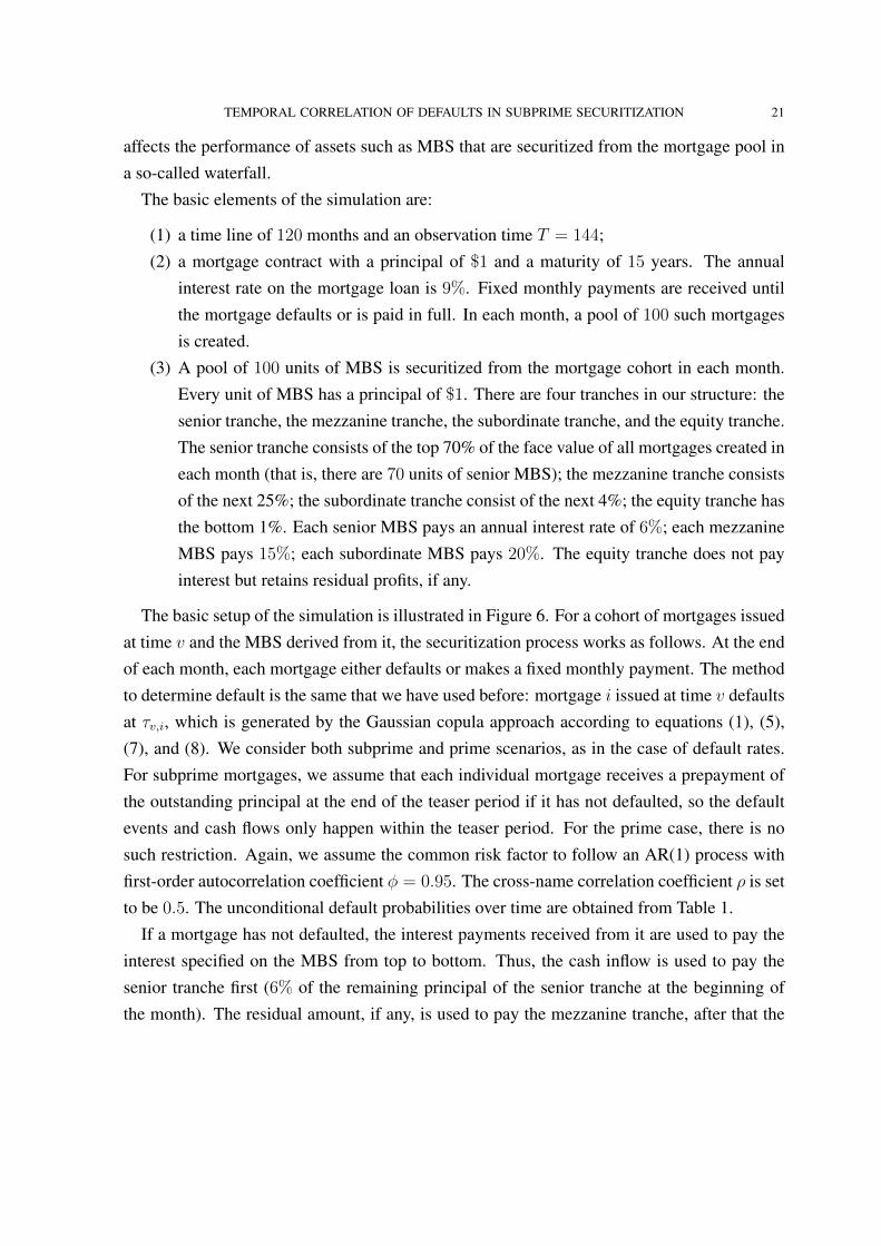
affects the performance of assets such as MBS that are securitized from the mortgage pool ina so-called waterfall.

The basic elements of the simulation are:

(1) a time line of 120 months and an observation time T = 144;(2) a mortgage contract with a principal of $1 and a maturity of 15 years. The annual

interest rate on the mortgage loan is 9%. Fixed monthly payments are received untilthe mortgage defaults or is paid in full. In each month, a pool of 100 such mortgagesis created.

(3) A pool of 100 units of MBS is securitized from the mortgage cohort in each month.Every unit of MBS has a principal of $1. There are four tranches in our structure: thesenior tranche, the mezzanine tranche, the subordinate tranche, and the equity tranche.The senior tranche consists of the top 70% of the face value of all mortgages created ineach month (that is, there are 70 units of senior MBS); the mezzanine tranche consistsof the next 25%; the subordinate tranche consist of the next 4%; the equity tranche hasthe bottom 1%. Each senior MBS pays an annual interest rate of 6%; each mezzanineMBS pays 15%; each subordinate MBS pays 20%. The equity tranche does not payinterest but retains residual profits, if any.

The basic setup of the simulation is illustrated in Figure 6. For a cohort of mortgages issuedat time v and the MBS derived from it, the securitization process works as follows. At the endof each month, each mortgage either defaults or makes a fixed monthly payment. The methodto determine default is the same that we have used before: mortgage i issued at time v defaultsat τv,i, which is generated by the Gaussian copula approach according to equations (1), (5),(7), and (8). We consider both subprime and prime scenarios, as in the case of default rates.For subprime mortgages, we assume that each individual mortgage receives a prepayment ofthe outstanding principal at the end of the teaser period if it has not defaulted, so the defaultevents and cash flows only happen within the teaser period. For the prime case, there is nosuch restriction. Again, we assume the common risk factor to follow an AR(1) process withfirst-order autocorrelation coefficient φ = 0.95. The cross-name correlation coefficient ρ is setto be 0.5. The unconditional default probabilities over time are obtained from Table 1.

If a mortgage has not defaulted, the interest payments received from it are used to pay theinterest specified on the MBS from top to bottom. Thus, the cash inflow is used to pay thesenior tranche first (6% of the remaining principal of the senior tranche at the beginning ofthe month). The residual amount, if any, is used to pay the mezzanine tranche, after that the

22 E. HILLEBRAND, A. SENGUPTA, AND J. XU

subordinate tranche, and any still remaining funds are collected in the equity tranche. If thecash inflow passes a tranche threshold but does not cover the following tranche, it is proratedto the following tranche. Any residual funds after all the non-equity tranches have been paidadd to the principal of the equity tranche. Principal payments are processed analogously. Weassume a recovery rate of 50% on the outstanding principal for defaulted mortgages. The 50%

loss of principal is deducted from the principal of the lowest ranked outstanding MBS. Thismeans that the equity tranche covers the principal loss first. If there is no principal left inthe equity tranche, the subordinate tranche covers the remaining loss and so on upwards. Inorder to capture MBS price performance through time, we calculate the present value of allcash flows received from each MBS tranche and average across 1000 simulations. This resultsin a time series of expected present values and can be viewed as a proxy for tranche priceevolution.

Before we examine the vintage correlation of the present value of MBS tranches, we look atthe time series of total principal loss across MBS tranches. In our simulations, no loss of prin-cipal occurred for the senior tranche. The series of expected principal losses of other tranchesand their sample autocorrelation and sample partial autocorrelation are plotted in Figures 7and 8 for subprime and prime scenarios respectively. We use the same method to obtain theautocorrelation functions for prime mortgages as in the case of default rates. The correlogramsshow that the expected loss of principal for each tranche follows an AR(1) process, althoughthe estimated coefficients are smaller than φ = 0.95, the first-order autocorrelation coefficientof Zv, in all cases.

The series of present values of cash flows for each tranche and their sample autocorrelationand partial autocorrelation functions are plotted in Figures 9 and 10 for subprime and primescenarios, respectively. The senior tranche displays a significant first-order autocorrelationcoefficient due to losses in interest payments although there are no losses in principal. Thepartial autocorrelation functions, which have significant positive values for more than one lag,suggest that the cash flows may not follow an AR(1) process due to the high non-linearity.However, the estimated vintage correlation still decreases over vintages, same as in an AR(1)process, which indicates that our findings for default rates can be extended to cash flows.

TEMPORAL CORRELATION OF DEFAULTS IN SUBPRIME SECURITIZATION 23

5. CONCLUSIONS

Default rates of subprime mortgages exhibit temporal correlation. Default events of subprime-mortgages depend on house price changes that are serially correlated, and this serial correla-tion is inherited by the sequence of defaults. We model a house price index by a common riskfactor in a Gaussian copula model. Analytical findings and simulations show that credit assetsinherit correlation of defaults across different vintages of initiation from serial correlation inthe common risk factor. The same is true in waterfall structures, used in mortgage-backedsecurities and collateralized debt obligations. Simulation results demonstrate that when thecommon risk factor of different cohorts of individual mortgages is serially correlated, theprice of the MBS securitized from these mortgages also displays serial correlation. Thesefindings are consistent with the view that the current financial crisis, which was triggered by alarge and serially correlated arrival of subprime mortgage defaults, has its origin in the declineof the housing market.

ACKNOWLEDGMENTS

Discussions with Darrell Duffie and Jean-Pierre Fouque helped improve the paper. Wethank seminar and conference participants at Stanford University, UC Merced, UC Riverside,UC Santa Barbara, and the 2010 Midwest Econometrics Group Meetings in St. Louis.

REFERENCES

ANDERSEN, L., AND J. SIDENIUS (2005): “Extensions to the Gaussian Copula: Random Recovery and Ran-dom Factor Loadings,” Journal of Credit Risk, 1(1), 29–70.

ANDERSEN, L., J. SIDENIUS, AND S. BASU (2003): “All your Hedges in One Basket,” Risk, November, 67–72.BAJARI, P., C. CHU, AND M. PARK (2008): “An Empirical Model of Subprime Mortgage Default From 2000to 2007,” Working Paper 14358, NBER.

BEARE, B. (2010): “Copulas and Temporal Dependence,” Econometrica, 78(1), 395–410.BERD, A., R. ENGLE, AND A. VORONOV (2007): “The Underlying Dynamics of Credit Correlations,” Journalof Credit Risk, 3(2), 27–62.

BLUHM, C., L. OVERBECK, AND C. WAGNER (2002): An Introduction to Credit Risk Modeling, FinancialMathematics Series. Chapman & Hall/CRC, London, UK.

BURTSCHELL, X., J. GREGORY, AND J.-P. LAURENT (2009): “A Comparative Analysis of CDO Pricing Mod-els,” Journal of Derivatives, 16(4), 9–37.

CABALLERO, R. J., AND A. KRISHNAMURTHY (2009): “Global Imbalances and Financial Fragility,” AmericanEconomic Review, 99(2), 584–588.

CROUHY, M. G., R. A. JARROW, AND S. M. TURNBULL (2008): “The Subprime Credit Crisis of 2007,”Journal of Derivatives, 16(1), 81–110.

24 E. HILLEBRAND, A. SENGUPTA, AND J. XU

DAGLISH, T. (2009): “What Motivates a Subprime Borrower to Default?,” Journal of Banking and Finance,33(4), 681–693.

DAS, S. R., L. FREED, G. GENG, AND N. KAPADIA (2006): “Correlated Default Risk,” Journal of FixedIncome, 16(2), 7–32.

DUFFIE, D., AND K. SINGLETON (2003): Credit Risk: Pricing, Measurement, and Management, PrincetonSeries in Finance. Princeton University Press, Princeton, NJ.

FIGLEWSKI, S. (2009): “Viewing the Crisis from 20,000 Feet Up,” Journal of Derivatives, 16(3), 53–61.FREES, E. W., AND E. A. VALDEZ (1998): “Understanding Relationships Using Copulas,” North AmericanActuarial Journal, 2(1), 1–25.

FREY, R., AND A. MCNEIL (2003): “Dependent Defaults in Models of Portfolio Credit Risk,” Journal of Risk,6(1), 59–92.

GIESECKE, K. (2003): “A Simple Exponential Model for Dependent Defaults,” Journal of Fixed Income, 13(3),74–83.

GORTON, G. (2008): “The Panic of 2007,” Working Paper 14358, NBER.(2009): “Information, Liquidity, and the (Ongoing) Panic of 2007,” American Economic Review, 99(2),

567–572.GRAZIANO, G. D., AND L. C. G. ROGERS (2009): “A Dynamic Approach to the Modeling of CorrelationCredit Derivatives Using Markov Chains,” International Journal of Theoretical and Applied Finance, 12(1),45–62.

HAYRE, L. S., M. SARAF, R. YOUNG, AND J. CHEN (2008): “Modeling of Mortgage Defaults,” Journal ofFixed Income, 17(4), 6–30.

HULL, J., M. PREDESCU, AND A. WHITE (2009): “The Valuation of Correlation-Dependent Credit DerivativesUsing a Structural Model,” Working paper.

HULL, J., AND A. WHITE (2001): “Valuing Credit Default Swaps II: Modeling Default Correlations,” Journalof Derivatives, 8(3), 12–22.

LANDO, D. (2004): Credit Risk Modeling: Theory and Applications, Princeton Series in Finance. PrincetonUniversity Press, Princeton, NJ.

LAURENT, J., AND J. GREGORY (2005): “Basket Default Swaps, CDOs and Factor Copulas,” Journal of Risk,7(4), 103–122.

LI, D. (2000): “On Default Correlation: A Copula Function Approach,” Journal of Fixed Income, 9(4), 43–54.LINDSKOG, F., AND A. MCNEIL (2003): “Common Poisson Shock Models: Applications to Insurance andCredit Risk Modelling,” ASTIN Bulletin, 33(2), 209–238.

MURPHY, D. (2008): “A Preliminary Enquiry into the Causes of the Credit Crunch,” Quantitative Finance, 8(5),435–451.

REINHART, C. M., AND K. S. ROGOFF (2008): “Is the US Sub-Prime Financial Crisis So Different? AnInternational Historical Comparison,” American Economic Review, 98(2), 339–344.

(2009): “The Aftermath of Financial Crises,” American Economic Review, 99(2), 466–472.SCHONBUCHER, P. (2003): Credit Derivatives Pricing Models: Models, Pricing and Implementation. Wiley,Chichester, UK.

TEMPORAL CORRELATION OF DEFAULTS IN SUBPRIME SECURITIZATION 25

SCHONBUCHER, P., AND D. SCHUBERT (2001): “Copula Dependent Default Risk in Intensity Models,” Work-ing paper, Bonn University.

SERVIGNY, A., AND O. RENAULT (2002): “Default Correlation: Empirical Evidence,” Working paper, Standardand Poor’s.

SIDENIUS, J., V. PITERBARG, AND L. ANDERSEN (2008): “A New Framework for Dynamic Credit PortfolioLoss Modelling,” International Journal of Theoretical and Applied Finance, 11(2), 163–197.

SKLAR, A. (1959): “Fonctions de Repartition a n Dimensions et Leurs Marges,” Publ. Inst. Stat. Univ. Paris, 8,229–231.

26 E. HILLEBRAND, A. SENGUPTA, AND J. XU

TABLE 1. Default Probabilities Through Time (F (τ)).

SubprimeTime (Month) 12 24 36 72 144Default Probability 0.04 0.10 0.12 0.13 0.14

PrimeTime (Month) 12 24 36 72 144Default Probability 0.01 0.02 0.03 0.04 0.05

FIGURE 1. Two-Year Changes in U.S. House Price and Subprime ARMSerious Delinquency Rates

2002 2003 2004 2005 2006 2007 2008 2009−100

−50

0

50US Home Price Index Changes (Two−Year Rolling Window)

2002 2003 2004 2005 2006 2007 2008 20090

10

20

30

40US Subprime Adjustable−Rate−Mortgage Serious Delinquency Rates (%)

“U.S. home price two-year rolling changes” are two-year overlapping changes in the S&P Case-Shiller U.S.National Home Price index. “Subprime ARM Serious Delinquency Rates” are obtained from the MortgageBanker Association. Both series cover the first quarter in 2002 to the second quarter in 2009.

TEMPORAL CORRELATION OF DEFAULTS IN SUBPRIME SECURITIZATION 27

FIGURE 2. Correlation of pv and pv′ when X∗ = −2

0 0.5 10

0.5

1ρ=0.1

φj

corr

0 0.5 10

0.5

1ρ=0.2

φj

corr

0 0.5 10

0.5

1ρ=0.3

φj

corr

0 0.5 10

0.5

1ρ=0.4

φj

corr

0 0.5 10

0.5

1ρ=0.5

φj

corr

0 0.5 10

0.5

1ρ=0.6

φj

corr

0 0.5 10

0.5

1ρ=0.7

φj

corr

0 0.5 10

0.5

1ρ=0.8

φj

corr

0 0.5 10

0.5

1ρ=0.9

φjco

rrCorrelation between pv and pv′ as a function of φ for different scenarios of the cross-mortgage correlationparameter ρ ∈ (0, 1). X∗ is set to −2 in all scenarios.

FIGURE 3. Correlation of pv and pv′ when X∗ = 0

0 0.5 10

0.5

1ρ=0.1

φj

corr

0 0.5 10

0.5

1ρ=0.2

φj

corr

0 0.5 10

0.5

1ρ=0.3

φj

corr

0 0.5 10

0.5

1ρ=0.4

φj

corr

0 0.5 10

0.5

1ρ=0.5

φj

corr

0 0.5 10

0.5

1ρ=0.6

φj

corr

0 0.5 10

0.5

1ρ=0.7

φj

corr

0 0.5 10

0.5

1ρ=0.8

φj

corr

0 0.5 10

0.5

1ρ=0.9

φj

corr

Correlation between pv and pv′ as a function of φ for different scenarios of the cross-mortgage correlationparameter ρ ∈ (0, 1). X∗ is set to 0 in all scenarios.

28 E. HILLEBRAND, A. SENGUPTA, AND J. XU

FIGURE 4. Serial Correlation in Default Rates of Subprime Mortgages

0 20 40 60 80 100 1200.08

0.1

0.12Default Rates Across Vintages

0 2 4 6 8 10 12 14 16 18 20−0.5

0

0.5

1

Lag

Vintage Correlation

0 2 4 6 8 10 12 14 16 18 20−0.5

0

0.5

1

Lag

Sample Partial Autocorrelation Function

FIGURE 5. Serial Correlation in Default Rates of Prime Mortgages

0 20 40 60 80 100 1200.02

0.04

0.06Default Rates Across Vintages

0 2 4 6 8 10 12 14 16 18 20−0.5

0

0.5

1

Lag

Vintage Correlation

0 2 4 6 8 10 12 14 16 18 20−0.5

0

0.5

1

Lag

Sample Partial Autocorrelation Function

TEMPORAL CORRELATION OF DEFAULTS IN SUBPRIME SECURITIZATION 29

FIGURE 6. Simulated Mortgages and MBS

M1

MortgagePool

M2

M3

M4

Principal: $1;Annual interestrate: 9%;Maturity: 15years.

A TypicalMortgage

M99

M100

Senior70%

Mezzanine25%

Subordinate4%

Equity1%

MBSInterest

Rate

6%

15%

20%

N/A

$$$

$$$

$$$

$$$

$$$

$$$

1 2 3 4 v V = 120 T = 144

30 E. HILLEBRAND, A. SENGUPTA, AND J. XU

FIGURE 7. Serial Correlation in Principal Losses of Subprime MBS

0 5 10−0.5

0

0.5

1

Vin

tage

Cor

r

Mezzanine Tranche

0 5 10−0.5

0

0.5

1

Par

tial A

utoc

orr

0 5 10−0.5

0

0.5

1Subordinate Tranche

0 5 10−0.5

0

0.5

1

0 5 10−0.5

0

0.5

1Equity Tranche

0 5 10−0.5

0

0.5

1

The first row plots the vintage correlation of the principal loss of each tranche. The correlation is estimated usingthe sample autocorrelation function. The second row plots the partial autocorrelation functions.

FIGURE 8. Serial Correlation in Principal Losses of Prime MBS

0 10 20−0.5

0

0.5

1

Vin

tage

Cor

r

Mezzanine Tranche

0 10 20−0.5

0

0.5

1

Par

tial A

utoc

orr

0 10 20−0.5

0

0.5

1Subordinate Tranche

0 10 20−0.5

0

0.5

1

0 10 20−0.5

0

0.5

1Equity Tranche

0 10 20−0.5

0

0.5

1

The first row plots the vintage correlation of the principal loss of each tranche. The correlation is estimated usingthe correlation between the first and subsequent vintages, each of which has a Monte Carlo sample size of 1000.The second row plots the partial autocorrelation functions of the demeaned series of principal losses.

TEMPORAL CORRELATION OF DEFAULTS IN SUBPRIME SECURITIZATION 31

FIGURE 9. Cash Flows from Subprime MBS

0 5 10−0.5

0

0.5

1

Vin

tage

Cor

r

Senior

0 5 10−0.5

0

0.5

1

Par

tial A

utoc

orr

0 5 10−0.5

0

0.5

1Mezzanine

0 5 10−0.5

0

0.5

1

0 5 10−0.5

0

0.5

1Subordinate

0 5 10−0.5

0

0.5

1

0 5 10−0.5

0

0.5

1Equity

0 5 10−0.5

0

0.5

1

The first row plots the vintage correlation of the cash flow received by each tranche. The correlation is estimatedusing the sample autocorrelation function. The second rows plot the partial autocorrelation functions.

FIGURE 10. Cash Flows from Prime MBS

0 10 20−0.5

0

0.5

1

Vin

tage

Cor

r

Senior

0 10 20−0.5

0

0.5

1

Par

tial A

utoc

orr

0 10 20−0.5

0

0.5

1Mezzanine

0 10 20−0.5

0

0.5

1

0 10 20−0.5

0

0.5

1Subordinate

0 10 20−0.5

0

0.5

1

The first row plots the vintage correlation of the cash flow received by each tranche. The correlation is estimatedusing the correlation between the first and subsequent vintages, each of which has a Monte Carlo sample size of1000. The second row plots the partial autocorrelation functions of the demeaned series of cash flow.

32 E. HILLEBRAND, A. SENGUPTA, AND J. XU

(E. Hillebrand) DEPARTMENT OF ECONOMICS, LOUISIANA STATE UNIVERSITY, BATON ROUGE, USA.E-mail address: erhil@lsu.edu

(A. Sengupta) DEPARTMENT OF MATHEMATICS, LOUISIANA STATE UNIVERSITY, BATON ROUGE, USA.E-mail address: ambarnsg@yahoo.com

(J. Xu) DEPARTMENT OF ECONOMICS, LOUISIANA STATE UNIVERSITY, BATON ROUGE, USA.E-mail address: jxu2@tigers.lsu.edu