TEMPORAL AGGREGATION OF AN ESTAR PROCESS: SOME IMPLICATIONS

FOR PURCHASING POWER PARITY ADJUSTMENT *

Ivan Payá and David A. Peel **

WP-AD 2004-25

Corresponding author: Ivan Payá, Departamento Fundamentos Análisis Económico, University of Alicante, 03080 Alicante, Spain. E-mail address: ivanpaya@merlin.fae.ua.es Tel.: +34 965903614. Fax: +34 965903898 Editor: Instituto Valenciano de Investigaciones Económicas, S.A. Primera Edición Junio 2004. Depósito Legal: V-3007-2004 IVIE working papers offer in advance the results of economic research under way in order to encourage a discussion process before sending them to scientific journals for their final publication.

* The authors are grateful for helpful and constructive comments to the editor and two anonymous referees. The authors are grateful to participants of the Understanding Evolving Macroeconomy Annual Conference, University College Oxford 15-16 September 2003. I. Payá acknowledges financial support from the Instituto Valenciano de Investigaciones Economicas (IVIE). David Peel gratefully acknowledges financial support by ESRC grant L/138/25/1004. ** I. Payá: Departamento Fundamento Analisis Economico, University of Alicante, 03080 Alicante, Spain E-mail address: ivanpaya@merlin.fae.ua.es Tel.: +34 965903614. Fax: +34 965903898. D. A. Peel: Lancaster University Management School, Lancaster, LA1 4YX, UK, United Kingdom.

2

TEMPORAL AGGREGATION OF AN ESTAR PROCESS: SOME IMPLICATIONS

FOR PURCHASING POWER PARITY ADJUSTMENT

Ivan Payá and David A. Peel

ABSTRACT

Nonlinear models of deviations from PPP have recently provided an important,

theoretically well motivated, contribution to the PPP puzzle. Most of these studies use

temporally aggregated data to empirically estimate the nonlinear models. As noted by Taylor

(2001), if the true DGP is nonlinear, the temporally aggregated data could exhibit misleading

properties regarding the adjustment speeds. We examine the effects of different levels of

temporal aggregation on\ estimates of ESTAR models of real exchange rates. Our Monte

Carlo results show that temporal aggregation does not imply the disappearance of nonlinearity

and that adjustment speeds are significantly slower in temporally aggregated data than in the

true DGP. Furthermore, the autoregressive structure of some monthly ESTAR estimates

found in the literature is suggestive that adjustment speeds are even faster than implied by the

monthly estimates.

Keywords: ESTAR, Real Exchange Rate, Purchasing Power Parity, Aggregation.

JEL classification: F31, C22, C51

1 Introduction

At the time of publication of Rogoff’s (1996) influential survey on PurchasingPower Parity (PPP), almost without exception, the vast amount of empir-ical work reported was based on a linear framework. The empirical resultsconcerning the mean-reverting properties of PPP deviations were contradic-tory. Whilst on the basis of standard unit root tests, the majority of studiesreported that real exchange rate deviations were mean reverting, I(0) pro-cesses, a significant number of studies reported that they were described bynon mean-reverting, I(1), processes. Other studies reported that PPP devi-ations were parsimoniously described by mean reverting fractional processesthat exhibited the long memory associated with this process (see e.g., Dieboldet al., 1991; and Cheung and Lai, 1993)2.Though the literature on this issue disagreed on the appropriate degree

of integration of PPP deviations it did have a common feature. Short runPPP deviations were undoubtedly very persistent. In his review, Rogoff(1996) concluded that, on balance, the implied speed of adjustment of PPPdeviations to shocks was “glacially slow”. This fact constituted a puzzlegiven the half life of shocks was some 3-5 years, seemingly far too long to beexplained by nominal rigidities.Since 1996 a number of papers have reported empirical results which pro-

vide some explanation of the contradictory empirical results obtained whenemploying the linear methodology. In these papers PPP deviations are par-simoniously modelled employing two nonlinear models, namely the thresholdmodel of Tong (1990), and the Exponential Smooth Autoregressive model(ESTAR) model of Ozaki (1985) (see e.g., Michael et al., 1997; Obstfeld andTaylor, 1997; Taylor et al., 2001; and Kilian and Taylor, 2003). Whilst glob-ally mean-reverting these nonlinear processes have the property of exhibitingnear unit root behavior for small deviations from PPP. This type of nonlin-ear adjustment process captures the adjustment derived in the theoreticalanalyses of PPP by a number of authors (see e.g., Dumas, 1992; Sercu etal., 1995; O’Connell, 1998; and Berka, 2002). These theoretical analyses of

2Fractional processes allow the degree of integration of a series to be non-integer.Standard unit root tests may exhibit low power against the fractional alternative. Thefractional processes are given by members of the class of ARFIMA(p, d, q) processes,xt(1− L)d = ut, where ut is a stationary ARMA(p, q) process, and d is non-integer. Theautocorrelations of the fractional process exhibit hyperbolic rather than geoemetric decay.For 0.5≤d<1 the process is non-stationary but mean reverting.

3

PPP demonstrate how transactions costs, transport costs or the sunk costsof international arbitrage induce nonlinear adjustment of the real exchangerate. Essentially small deviations from PPP are left uncorrected if they arenot large enough to cover the costs of international arbitrage.The nonlinear models can provide both an explanation of the contra-

dictory results reported on the integration properties of PPP deviations aswell as providing a different perspective on adjustment speeds. Taylor etal. (2001) and Pippenger and Goering (1993) demonstrate that the standardDickey Fuller unit root tests have low power against data simulated from anESTAR model. Byers and Peel (2000, 2003) show that data that is gener-ated from an ESTAR process can appear to exhibit the fractional property.That this would be the case was an early conjecture by Acosta and Granger(1995). Given that the ESTAR model has a theoretical rationale, whilst thefractional process is, from an economic perspective, a relatively non intuitiveprocess, the apparent fractional property of PPP deviations might reasonablybe interpreted as a misspecification of a linear model relative to the DGP.3

An important property of the nonlinear models is that the impulse re-sponse functions derived from them show that, whilst the speed of adjustmentfor small shocks around equilibrium can be extremely slow, larger shocksmean-revert much faster than the “glacial rates” obtained in the linear es-timates (see e.g., Taylor et al., 2001; and Paya et al., 2003). Consequentlynonlinear models provide a theoretically well motivated and therefore impor-tant contribution to explaining the PPP speed of adjustment puzzle outlinedin Rogoff (1996).One issue not discussed in previous analysis is how temporal aggregation

will impact on the adjustment speed obtained from estimates of non linearmodels. Taylor (2001) demonstrates that if the true data generating processis a nonlinear threshold process, and if the data employed in estimation istemporally aggregated, then linear estimates of adjustment speeds can besubstantially downward biased. He does not consider the implications oftemporal aggregation for estimates of adjustment speeds if the true datagenerating process is a nonlinear process but a nonlinear model is estimatedon the temporally aggregated data. This issue seems to be of interest fortwo reasons. First, as noted by Taylor (2001), much of the data employedin PPP empirical work is temporally aggregated. Second, in the recent PPPliterature estimates of nonlinear models have been reported employing data

3See Granger and Terasvirta (1999).

4

sampled at different levels of aggregation. For example, employing the ES-TAR form, Baum et al. (2001), and Taylor et al. (2001) report resultsemploying monthly data, Kilian and Taylor (2003) quarterly data whilstMichael et al. (1997), and Paya and Peel (2003a) report results employingannual data.4 If the true data generating process (DGP) is nonlinear, it isclearly of interest to examine the nature of the nonlinear models that occurin temporally aggregated data. Conditional on the assumed DGP the resultsobtained may shed light on the appropriate frequency of the adjustment pro-cess in actual data. In addition, we can compare and contrast the estimatedspeeds of adjustment obtained in the DGP and the temporally aggregatedprocess.5

These are the purposes in this article. We assume, based on a prioriconsiderations, that at the very highest data frequency the true DGP is givenby a particular, theoretically well motivated, ESTAR model. A Monte Carloanalysis is conducted where we estimate ESTAR models derived from thisDGP at various degrees of temporal aggregation. The important point toemerge is that, for the particular DGP assumed, temporal aggregation doesnot lead, in general, to the disappearance of nonlinearity. In addition, thetemporally aggregated models exhibit a different ESTAR form to that in theDGP and which is precisely that found in empirical estimates of quarterlyand annual data. Given that the DGP is as postulated we can infer fromestimates based on monthly data whether temporal aggregation has occurredwith consequent implications for adjustment speeds. We find that adjustmentspeeds implied in the temporally aggregated data are much slower than theadjustment speeds obtained in the true DGP and that true adjustment speedsmay be faster than those derived from monthly data, the highest frequencyavailable to us.The rest of the paper is organized as follows. In section 2 we set out

the DGP for highest frequency data, our Monte Carlo methodology, and theeffect of temporal aggregation on nonlinear estimates of an ESTAR model.Section 3 compares the Monte Carlo results with actual estimates. In section4 we examine, employing nonlinear impulse response functions, the speedsof adjustment to shocks obtained in the DGP and the estimated temporally

4In related work on the monetary model of exchange rate determination Taylor andPeel (2000) estimate an ESTAR model on quarterly data.

5Very little work has been done on the effects of aggregation on Non-linear time seriesmodels. Granger (1991), and Granger and Lee (1999) are notable exceptions. Howevertheir analysis does not consider nonlinear processes involving symmetric adjustment.

5

aggregated ESTAR models. Finally, section 5 summarizes our main conclu-sions.

2 The True Structural Model and the Effectof Time Aggregation on estimated nonlin-ear parameters

We assume that at the highest frequency the DGP is given by an ExponentialSmooth Autoregressive model (ESTAR) model of Ozaki (1985). A smoothrather than discrete adjustment mechanism is chosen for two reasons. First asmooth adjustment process is suggested by the theoretical analysis of Dumas(1992). Second, as postulated by Terasvirta (1994) and demonstrated theo-retically by Berka (2002), in aggregate data, regime changes may be smoothrather than discrete given that heterogeneous agents do not act simultane-ously even if they make dichotomous decisions.6 The relevant ESTAR modelwhich is, a priori, appropriate for modelling PPP deviations at the highestdata frequency has the simplest possible structure within the class of ESTARmodels and is given by

yt = e−γy2t−1yt−1 + ut (1)

where γ is a positive constant and ut is a white noise disturbance term.Figure 1 is a deterministic plot of the relationship between ∆y = yt−yt−1

and yt−1 obtained from (1). We observe in Figure 1 that for small deviationsfrom equilibrium, adjustment may be modelled as a unit root process - “theoptimality of doing nothing” - but for large deviations from equilibrium thereis mean reversion. If the process spends a significant proportion of time inor near the unit root region, it will exhibit strong persistence and near unitroot behavior. It is also interesting to note that the form of ESTAR modelwe assume is precisely that which has been found to provide a parsimoniousfit to many monthly data sets.

6Even in high frequency asset markets the idea of heteregeneous traders facing differentcapital constraints or percieved risk of arbitrage has been employed to rationalise employ-ment of the ESTAR model. See, e.g. Tse (2001) for arbitrage between stock and indexfutures.

6

We simulate data from the ESTARmodel (1) where the disturbance term,ut, is assumed to be normally distributed7.Following Taylor (2001) we create arithmetic temporal aggregates from

the simulated data as8

y∗t =(yt + yt−1 + yt−2 + ......+ yt−i)

i(2)

where i = 2, 3, 12.

Two different assumptions about the true DGP are made. First, weassume that the true DGP is a nonlinear ‘monthly’ ESTAR process andsimulate from this 120,000 observations. We replicate this experiment 1,000times.The range of standard deviations of the disturbance term is calibrated on

the monthly estimates of equation (1), the highest aggregate data frequencyavailable to researchers (see e.g., Taylor et al., 2001; and Venetis et al., 2002).These studies report standard deviations (σ) of around 0.035. For purposesof comparison we also simulate series with a much lower standard deviationthan found in the monthly data and employ values of σ of 0.01 and 0.035.The adjustment parameter is given the values of γ = 0.5, 1. The estimatesobtained in actual monthly data tend to fall in this range.Aggregating these observations three times, i = 3 (quarterly), or twelve

times, i = 12 (annual), yields 1,000 samples of 40,000 and 10,000 observa-tions respectively. These samples will be used to analyze the ‘large sample’behavior of aggregated nonlinear ‘monthly’ ESTAR models. To analyze thesmall sample properties, we employ the same method but limit the sample

7We also consider nonnormal disturbances such as t-Student with 18 degrees of freedomthat in previous research appears to match the nonnormality of residuals (see Paya andPeel 2003b). Results were qualitatively unchanged.

8If the data is in logarithmic form, then y∗t is the geometric mean instead of the arith-metic mean of the real exchange rates. We compared the correlation between the arith-metic and geometric means conditional on some price processes. The correlations wereclose to unity and the results qualitatively similar. Given this for simplicity we followTaylor (2001) and employ the arithmetic mean for the temporally aggregated data.

7

sizes to 120 for ‘quarterly’ (i = 3) aggregation and 200 for ‘annual’ (i = 12)as these span the most common used samples in the literature.9

The second assumption made is that the true DGP given by (1) is for datagenerated at either a fortnightly or ten days frequency that is aggregated tomonthly data (i = 2, or 3) respectively. Again 120,000 observations are sim-ulated from (1) 1,000 times. In this case the standard errors of the residualsin the true DGP are chosen as σ = 0.024, 0.028 so that the standard errorsof the residuals in the temporally aggregated data, i = 2, i = 3 match thosefound in actual monthly estimates. Values of γ = 0.3, 0.4 were employedwhich produced values of the speed of adjustment parameter in the aggre-gate data similar to those observed in empirical work. In this exercise, thelarge sample analysis was done with 10,000 observations of the aggregateddata10 and the small sample analysis with 360 observations matching thesample size of monthly data on real exchange rates available from the postBretton Woods period and around the length of sample that has typicallybeen employed in previous empirical analysis.On the aggregated data we estimate by nonlinear least squares the fol-

lowing model

y∗t = a+B(L)y∗t−1e

−γ(y∗t−1−a)2 + vt (3)

where B(L) is a polynomial lag operator of order up to five which ren-dered the disturbance term vt empirical white noise,11 and a is a constant.Empirical marginal significance levels of the estimated parameter γ has tobe obtained through Monte Carlo simulation as it is not defined under thenull. In particular, the model is assumed to follow a unit root linear autore-gressive process12 and then a nonlinear ESTAR specification (equation 3) isestimated, computing the appropriate confidence interval of significance forγ.

9Samples of real exchange rates of 120 at quarterly data are available for the postBretton-Woods period. At annual frequency the longest data set available is from 1792 inthe case of Dollar/Pound and Dollar/French Franc (see Lothian and Taylor 1996).10The results employing 60,000 or 40,000 appeared essentially the same than on a sample

using 10,000. We report results on samples of 10,000 as it was computationally much lesstime consuming.11On the basis of the LM test of Eitrheim and Terasvirta (1996).12The number of autoregressive terms and the calibration of the slope parameters and

variance were obtained through a first estimate of a linear autoregressive process (restrict-ing the parameters to add up to one).

8

First, we examine the results obtained in the case of the large samplesdescribed above. We observe in the results reported in Tables 1, 2a, 2b, and 3that time aggregation induces higher order autoregressive terms in the fittedmodels at lower frequencies than occur in the DGP. Moreover, the additionalautoregressive structure induced by time aggregation seems to have a limitingnumber of terms. The second order autoregressive term is always significant.Terms in an autoregressive process of order three are significant at least95% of the time except for i=2 when it falls to 59%. Higher order termsexhibit a steep fall in significance. The significance of the AR(4) parametervaries between 37% and 7% with that of the AR(5) parameter between 5-7%.The order of the autoregressive structure appears to be independent of therange of standard errors of the disturbance term and the speed of adjustmentparameters imposed in the true DGP in our simulations.The regression standard error and the point estimate of the speed of

adjustment parameter, γ, increase with the degree of aggregation. The speedof adjustment parameter is always significant in the large sample estimates.Another feature of the time aggregation is the finding of significant LM testfor ARCH. The greater the degree of aggregation and the higher the standarderror of the disturbance term in the DGP the more accentuated the finding ofa significant LM test for ARCH. Noting that the LM test for ARCH is a testfor model misspecification and that the errors in the DGP do not exhibitARCH, this suggests that specification (3) may become less parsimonious asan appropriate way of modelling the temporally aggregated process (1) as thedegree of aggregation increases. We also note that the lower the frequencyand the higher the standard error of the disturbance term the lower thegoodness of fit parameter R2.When the estimations are undertaken with smaller samples of observa-

tions of 120, 200 and 360,corresponding to quarterly, annual and monthlydata employed in empirical studies, the nonlinear estimates of (3) show thefollowing features. The fitted ESTAR exhibits significant AR(2) structurebetween 50 and 89 percent of the time for i=2,3,12 dependent upon the noiseand the speed of adjustment in the true DGP. Autoregressive terms of ordergreater than two are significant less than ten percent of times. SignificantLM tests for ARCH are not found in 90% of the fitted models. The esti-mated speed of adjustment parameter are higher than in the large samplesimulations with larger standard errors and approximately forty percent aresignificant at the 5% significance level. Consequently, small sample esti-mations of nonlinear ESTAR models on temporally aggregated data could

9

erroneously reject that the true DGP follows a nonlinear process.13

Nonlinear ESTAR models have been reported at various levels of aggre-gation and the reported empirical results conform with those obtained onthe simulated data. Kilian and Taylor (2003) report AR(2) structure in allESTAR models fitted to quarterly data for seven OECD economies. Michaelet al. (1997) report AR(2) structure employing annual data. No one has re-ported AR structure greater than two. Also significant LM tests for ARCHare rarely reported.

3 Further Comparison between SimulatedData and Empirical Estimates from ActualData

We now proceed to compare further the empirical results obtained from sim-ulated data with those obtained from actual data. Table 4 presents monthlyestimates of ESTAR models for seven bilateral real exchange rates againstthe Dollar in the post Bretton Woods era taken from Venetis et al. (2002).14

The estimated model corresponds to that of Equation (3). The estimates ofγ are between 0.16 and 0.8 and the standard deviation of the regressions isaround 0.033. We added the last column, where the p-value of the second ARterm in the estimates is included. For the majority of the cases, PPP devia-tions appear parsimoniously described by the simple ESTAR structure givenby equation (1). However, it appears that in the case of the Dollar/Yen atthe five percent, the Dollar/Pound and Dollar/Lira at the fifteen percent, thesecond AR term plays a significant role. Simulations presented above showthat time aggregation induces AR(2) structure in the estimated nonlinearprocess. The fact that some of the monthly models have significant secondAR terms could imply that the true ESTAR model is appropriate at evenhigher frequency than monthly. Of course, if there are already AR lags oforder two at the high-frequency DGP then this will not be the case. Howeverwe feel that AR lags of higher order than one at the high frequency DGP

13Granger and Lee (1999) examine the effects of time aggregation on nonlinearity testsdrawing a similar conclusion. Nonlinearity could be rejected when the model has beentemporally aggregated.14This represents the highest possible frequency on actual data on real exchange rates

as prices are provided monthly.

10

do not make apriori sense. The significance of this point will be ultimatelydetermined by whether higher order lags can be generated theoretically inthe DGP.Empirical results at different levels of aggregation (i = 3, i = 12) are

reported in Tables 5 and 6. The quarterly estimates are taken from Kil-ian and Taylor (2003) and we also present annual estimates of Equation(3) for Dollar/Pound and Dollar/Franc for two hundred years derived byLothian and Taylor (1996) and analyzed by Michael et al. (1997). The Dol-lar/Deutsche Mark is for the Gold Standard -data source- reported in Payaand Peel (2003a). We observe that the estimates of γ are higher than atmonthly frequency and similar to those suggested by the simulation exerciseabove. We also note that the autoregressive structures have a significantAR(2) component.15 This is interesting given our Monte Carlo showed thatin over fifty percent of simulations at “quarterly aggregation” and seventy fivepercent of simulations at “annual aggregation” gave rise to this specification.

4 Generalized impulse response functions

A number of properties of the impulse response functions of linear modelsdo not carry over to the nonlinear models. In particular, impulse responsesproduced by nonlinear models are; a) history dependent, so they depend oninitial conditions, b) dependent on the size and sign of the current shock, andc) they depend on future shocks as well. That is, nonlinear impulse responsescritically depend on the “past”, “present” and “future”.The Generalized Impulse Response Function (GIRF) introduced by Koop,

Pesaran and Potter (1996) successfully confronts the challenges that arise indefining impulse responses for nonlinear models. The impulse response isdefined as the average difference between two realizations of the stochasticprocess {yt+h} which start with identical histories up to time t − 1 (initialconditions) but one realization is “hit” by a shock at time t while for the other(the benchmark profile) no shock occurs. In a context similar to ours, Taylorand Peel (2000) conduct GIRF analysis on the deviations of real exchangerates from monetary fundamentals, and Baum et al. (2001), and Taylor et

15In the case of the Dollar/Franc the AR(2) term is insignificant but the residuals exhibitbetter properties. It is worth noting that these estimations span a long period of timewith different exchange rate regimes. However, those nonlinear estimates have recentlybeen proved to be robust (see Lothian and Taylor, 2004; and Paya and Peel, 2004).

11

al. (2001) use impulse response functions to gauge how long shocks survivein real exchange rate nonlinear models. The GIRF of Koop et al. (1996) isdefined as,

GIRFh(h, δ,ωt−1) = E(yt+h|ut = δ,ωt−1)−E(yt+h|ut = 0,ωt−1) (4)

where h = 1, 2, .., denotes horizon, ut = δ is an arbitrary shock occurringat time t and ωt−1 defines the history set of yt. Given that δ and ωt−1 aresingle realizations of random variables, expression (4) is considered to be arandom variable. In order to obtain sample estimates of (4), we averageout the effect of all histories ωt−1 that consist of every set (yt−1, ..., yt−p) fort ≥ p+1, where p is the autoregressive lag length, and we also average out theeffect of future shocks ut+h. In particular, for each available history we use300 repetitions to average out future shocks, where future shocks are drawnwith replacement from the models residuals, and then we average the resultacross all histories.16 We set the shocks on the log real exchange rate yt (equalto ln(1 + k/100) with k = 10, 20, 30) which correspond roughly to 10%, 20%and 30% shocks, respectively. The speed of real exchange rate convergencewill be measured with the half-life of shocks. In this case, the half-life ofshocks will be computed as the number of time periods that PPP deviationsneed to settle below 50% the size of the shock.17 Accordingly, we will reportthe half-lives of shocks defined as the time needed for GIRFh < 1

2δ.18

We examine the implied speeds of adjustment to shocks for the MonteCarlo experiments in Section 2 using the following procedure. First, wegenerate ESTAR DGP’s with given parameters γ, and standard deviationsof error term, se. These correspond to the highest frequency of the ‘true’process followed by PPP deviations. Following our discussion of the MonteCarlo simulations and empirical results in previous sections, we consider threecases: monthly, fortnightly and ten days. Parameters γ and se are fixedaccordingly. We estimate the models without aggregation and calculate theaverage half-life of shocks for those processes.

16We found out that the difference with using 500 repetitions was quantitatively in-significant. Without loss of generality, the impulse response horizon is set to max{h} = 48in the future.17For a full discussion on different measures of half-life shocks and estimating procedures

see Murray and Papell (2002) and Kilian and Zha (2002).18This is the same definition as in Taylor et al. (2001). However, please note that

half-life of shocks could also, in theory, be oscillatory.

12

Second, we aggregate the ‘true’ DGP at different levels: i = 3 and i = 12in the case of the ‘monthly’ true DGP; i = 2 in the case of ‘fortnight’ trueDGP; and i = 3 in the case of ‘ten days’ true DGP. We estimate the ESTARmodels as in Equation (3) and calculate the average half-life of shocks forthe cases where a significant estimate of γ is found.Table 7 reports the results of applying this procedure in the case of the

same large and small samples outlined above. For large samples, the halflife of shocks, for a 10% shock, is between 15 and 17 months for the trueDGP (lines 1, 4, and 6). However, the half-life of shocks of the temporallyaggregated data lie between 20 and 36 months (lines 2, 3, 5, and 7). Inthe case of small samples, for a 10% shock, the true DGPs exhibit half-livesbetween 6 and 13 months (lines 8, 11, and 13). The aggregated models showmuch lower adjustment responses, between 16 and 36 months (lines 9, 10,12, and 14).In order to compare our simulation results with actual estimates, Tables

8, 9 and 10 show the half-life shocks for the nonlinear models estimatedon actual data reported in Tables 4, 5 and 6. Employing the simulationsresults as a benchmark, we can then use these empirical estimates of half-lives of shocks to try to approximate the nature of the true DGP of PPPdeviations. We will concentrate on the speed of adjustment to shocks ofthe Dollar/Pound, Dollar/French Franc, and Dollar/Deutsche Mark. Thedifference between the speed of adjustment to shocks in the monthly andannual data is around twenty four months for the three different currencies.The difference between the adjustment at quarterly and annual data is eitherzero or twelve months. This pattern is the one followed by the Monte Carloresults when we aggregate a true DGP from monthly to quarterly and annualdata.

5 Conclusions

Taylor (2001) demonstrated that if the DGP is a nonlinear threshold pro-cess, and if the data employed in estimation is temporally aggregated, thenlinear estimates of adjustment speeds can be substantially downward biased.We have demonstrated in this article that a similar result holds for ESTARmodels estimated on temporally aggregated data when the true DGP is ES-TAR. In addition, if the true DGP is as postulated, the significance of morethan one autoregressive term in some monthly estimates raises the possibility

13

that adjustment speeds are even faster than obtained in monthly estimates.Consequently, temporal aggregation provides a further potential solution tothe speed of adjustment puzzle raised by Rogoff.

14

REFERENCES

Acosta, F.M. A., and C.W.J. Granger (1995), ‘A linearity test for nearfor near-unit root time series’. Discussion paper no. 95-12, University ofCalifornia San Diego, San Diego, CA.Baum, C.F., J.T. Barkoulas and M. Caglayan (2001), Nonlinear adjust-

ment to purchasing power parity in the post-Bretton Woods era’, Journal ofInternational Money and Finance, 20, 379-399.Berka, M. (2002), ‘General equilibrium model of arbitrage, trade and real

exchange rate persistence’. Mimeo. University of British Columbia.Byers, J.D., and D.A. Peel (2000), ‘Non-linear dynamics of inflation in

high inflation economies’, The Manchester School, 68, 23-37.Byers, J.D., and D.A. Peel (2003), ‘A nonlinear time series with mislead-

ing linear properties’, Applied Economics Letters, 10, 47-51Cheung, Y,W., and K.S. Lai (1993), ‘A fractional cointegration analysis

of purchasing power parity’, Journal of Business and Economic Statistics,11, 103-112.Diebold, F.X., S. Husted and M. Rush (1991), ‘Real exchange rates under

the gold standard’, Journal of Political Economy, 99, 1252-1271.Dumas, B. (1992), ‘Dynamic equilibrium and the real exchange rate in a

spatially separated world’, Review of Financial Studies, 5, 153-80.Eitrheim, O, and T. Terasvirta (1996), ‘Testing the adequacy of smooth

transition autoregressive models’, Journal of Econometrics, 74, 59-75.Granger, C.W.J. (1991), ‘Developments in the nonlinear analysis of eco-

nomic series’, Scandinavian Journal of Economics, 93, 263-272.Granger, C.W.J. and Lee (1999), ‘The effects of aggregation on nonlin-

earity’, In R,Mariano ed. Advances in Statistical Analysis and StatisaticalComputing, Greenwich JAI press.Granger, C.W.J. and T. Terasvirta (1999), ‘Ocasional structural breaks

and long memory’, UCSD Economics Discussion Paper 98-03.Kilian, L. and T. Zha (2002), ‘Quantifying the uncertainty about the half-

life of deviations from PPP’, Journal of Applied Econometrics, 17, 107-125.Kilian, L. and M.P. Taylor (2003), ‘Why is it so difficult to beat the

random walk for exchange rates?’, Journal of International Economics, 60,85-107Koop, G., M.H. Pesaran and S.M. Potter (1996), ‘Impulse response anal-

ysis in nonlinear multivariate models’, Journal of Econometrics, 74, 119-147

15

Lothian, J.R. and M.P. Taylor (1996), ‘Real exchange rate behavior: therecent float from the perspective of the past two centuries’. Journal of Po-litical Economy, 104, 488-509.Lothian, J.R., and M.P. Taylor (2004), ‘Real exchange rates over the past

two centuries: How important is the Harrod-Balassa-Samuelson effect?’.Michael, P., A.R. Nobay and D.A. Peel (1997), ‘Transactions costs and

nonlinear adjustment in real exchange rates: an empirical investigation’,Journal of Political Economy, 105, 862-879.Murray, C. and D. Papell (2002), ‘The purchasing power parity persis-

tence paradigm’, Journal of International Economics, 56, 1-19.Obstfeld, M. and A.M. Taylor (1997), ‘Nonlinear aspects of goods-market

arbitrage and adjustment : Hecksher’s commodity points revisited’, Journalof the Japanese and International Economies, 11, 441-479O’Connell, P. (1998), ‘Market frictions and real exchange rates’, Journal

of International Money and Finance, 17, 71-95.Ozaki, T. (1985), ‘Nonlinear time series models and dynamical systems’,

In E.J. Hannan, P.R. Krishnaiah, and M.M. Rao eds., Handbook of Statistics,V, Amsterdam, Elsevier, 25-83.Paya, I. and D.A. Peel (2003a), ‘Nonlinear PPP under the gold standard’,

Southern Economic Journal, forthcoming.Paya, I. and D.A. Peel (2003b), ‘On the relationship between nominal

exchange rates and domestic and foreign prices’, Mimeo, Cardiff BusinessSchool.Paya, I. and D.A. Peel (2004), ‘A new analysis of the determinants of

the real dollar-sterling exchange rate: 1871-1994’. Mimeo, Cardiff BusinessSchool.Paya, I., I.A. Venetis and D.A. Peel (2003), ‘Further evidence on PPP

adjusment speeds: The case of effective real exchange rates and the EMS’,Oxford Bulletin of Economics and Statistics, 65, 421-438.Pippenger, M.K. and G.Goering (1993), ‘A Note on the empirical power

of unit root tests under threshold processes’, Oxford Bulletin of Economicsand Statistics, 55, 473-81.Rogoff, K. (1996), ‘The purchasing power parity puzzle’, Journal of Eco-

nomic Literature, 34, 647-668Sercu,P., R. Uppal and C. Van Hull (1995), ‘The exchange rate in the

presence of transactions costs: Implications for tests of purchasing powerparity’, Journal of Finance, 50, 1309-1319.

16

Taylor, A.M. (2001), ‘Potential pitfalls for the purchasing power paritypuzzle? sampling and specification biases in mean-reversion tests of the lawof one price’, Econometrica, 69, 473-498.Taylor, M.P. and D.A. Peel (2000), ‘Nonlinear adjustment, long-run equi-

librium and exchange rate fundamentals’, Journal of International Moneyand Finance,19, 33-53Taylor, M.P., D.A. Peel, and L. Sarno (2001), ‘Nonlinear mean-reversion

in real exchange rates: Toward a solution to the purchasing power paritypuzzles’, International Economic Review, 42, 1015-1042.Terasvirta, T. (1994), ‘Specification, estimation and evaluation of smooth

transition autoregressive models’, Journal of the American Statistical Asso-ciation, 89, 208—218Tong, H. (1990), Non-linear time series: A dynamical system approach.

Oxford University Press.Tse, Y (2001), ‘Index arbitrage with heterogeneous investors: A smooth

transition error correction analysis’, Journal of Banking and Finance, 25,1829-1855.Venetis, I.A., I. Paya, I. and D.A. Peel (2002), ‘Do real exchange rates

’mean revert ’ to productivity? A nonlinear approach’, Mimeo, Cardiff Busi-ness School.

17

Table 1. Results for simulated aggregated data of ESTAR model

True DGP: yt = e−γy2t−1yt−1 + ut

Estimated model: y∗t = a+B(L)y∗t−1e

−γ(y∗t−1−a)2

Aggregation i=12 (annual aggregation)γ = 1 γ = 1se = 0.035 se = 0.01sample10, 000 sample 200 sample10, 000 sample 200

Mean γ 4.50 5.00 7.62 10.50sd γ 0.45 3.85 0.70 6.80t(γ) 1.000 0.240 1.000 0.370R2 0.60 0.60 0.86 0.85se 0.077 0.077 0.025 0.025LM Arch 1.000 0.183 0.300 0.070AR(2) 1.000 0.750 1.000 0.860AR(3) 0.995 0.095 0.990 0.120AR(4) 0.220 0.075 0.270 0.065AR(5) 0.070 0.070 0.060 0.060

γ = 0.50 γ = 0.50se = 0.035 se = 0.01sample10, 000 sample 200 sample10, 000 sample 200

Mean γ 2.78 3.30 4.07 5.95sd γ 0.24 2.00 0.38 4.58t(γ) 1.000 0.360 1.000 0.340R2 0.69 0.69 0.90 0.89se 0.082 0.082 0.026 0.026LM Arch 0.995 0.010 0.157 0.058AR(2) 1.000 0.770 1.000 0.840AR(3) 0.996 0.120 1.000 0.123AR(4) 0.220 0.080 0.290 0.067AR(5) 0.070 0.070 0.077 0.043Notes: sd denotes standard deviation of coefficient γ. t(γ) denotes ratio of significant γparameter where empirical significance level is obtained through Monte Carlo. se denotesstandard error of equation. LM Arch is the ratio of rejection of the Lagrange Multiplier testfor ARCH in the residuals. AR(p) denotes ratio of significant autoregressive termof order p

18

Table 2a. Results for simulated aggregated data of ESTAR model

True DGP: yt = e−γy2t−1yt−1 + ut

Estimated model: y∗t = a+B(L)y∗t−1e

−γ(y∗t−1−a)2

Aggregation i=3 (quarterly aggregation)γ = 1 γ = 1se = 0.035 se = 0.01sample 40, 000 sample 120 sample 40, 000 sample 120

Mean γ 2.14 3.50 2.37 13.80sd γ 0.09 3.00 0.17 19.50t(γ) 1.000 0.390 1.000 0.270R2 0.86 0.85 0.96 0.92se 0.047 0.047 0.013 0.013LM Arch 0.584 0.092 0.128 0.085AR(2) 1.000 0.460 1.000 0.510AR(3) 1.000 0.090 1.000 0.110AR(4) 0.370 0.066 0.350 0.083AR(5) 0.055 0.055 0.077 0.066

γ = 0.50 γ = 0.50se = 0.035 se = 0.01sample 40, 000 sample 120 sample 40, 000 sample 120

Mean γ 1.10 2.20 1.20 11.70sd γ 0.05 2.54 0.09 19.25t(γ) 1.000 0.375 1.000 0.240R2 0.90 0.88 0.97 0.92se 0.048 0.047 0.014 0.014LM Arch 0.310 0.070 0.127 0.087AR(2) 1.000 0.510 1.000 0.490AR(3) 1.000 0.100 1.000 0.090AR(4) 0.350 0.050 0.380 0.062AR(5) 0.070 0.070 0.068 0.078Notes: see notes in table 1

19

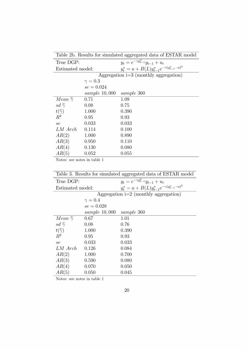
Table 2b. Results for simulated aggregated data of ESTAR model

True DGP: yt = e−γy2t−1yt−1 + ut

Estimated model: y∗t = a+B(L)y∗t−1e

−γ(y∗t−1−a)2

Aggregation i=3 (monthly aggregation)γ = 0.3se = 0.024sample 10, 000 sample 360

Mean γ 0.71 1.09sd γ 0.08 0.75t(γ) 1.000 0.390R2 0.95 0.93se 0.033 0.033LM Arch 0.114 0.100AR(2) 1.000 0.890AR(3) 0.950 0.110AR(4) 0.130 0.080AR(5) 0.052 0.055Notes: see notes in table 1

Table 3. Results for simulated aggregated data of ESTAR model

True DGP: yt = e−γy2t−1yt−1 + ut

Estimated model: y∗t = a+B(L)y∗t−1e

−γ(y∗t−1−a)2

Aggregation i=2 (monthly aggregation)γ = 0.4se = 0.028sample 10, 000 sample 360

Mean γ 0.67 1.01sd γ 0.08 0.76t(γ) 1.000 0.390R2 0.95 0.93se 0.033 0.033LM Arch 0.126 0.084AR(2) 1.000 0.700AR(3) 0.590 0.080AR(4) 0.070 0.050AR(5) 0.050 0.045Notes: see notes in table 1

20

Table 4. Results from ESTAR models of real exchange ratesmontly observations 1973-2001.

δ̂0 β̂1 β̂2 γ̂ s p AR(2)

FRF -0.025 1.037 β2 = 0 0.779 0.031 0.55(0.031) (0.022) (0.313)

BEF 0.005 1.018 β2 = 0 0.331 0.033 0.46(0.048) (0.020) (0.185)

DEM -0.027 1.033 β2 = 0 0.625 0.033 0.27(0.036) (0.021) (0.248)

ITL -0.045 1.017 β2 = 1− β1 0.336 0.030 0.15(0.043) (0.022) (0.194)

JPY 0.479 1.105 β2 = 1− β1 0.155 0.033 0.05(0.059) (0.053) (0.082)

NLG 0.041 1.022 β2 = 0 0.481 0.033 0.48(0.046) (0.022) (0.236)

GBP 0.109 1.094 β2 = 0 0.595 0.031 0.16(0.059) (0.069) (0.361)

Notes: Numbers in parentheses are Newey-West standard error estimates..

s denotes the residuals standard error. pAR(2) denotes p-value of secondautoregressive term.in the ESTAR estimation.

Source: Table from Venetis et al. (2002)

21

Table 5. Results from ESTAR models of real exchange ratesquarterly observations 1973.I-1998.IV

δ̂0 β̂1 β̂2 γ̂ s

FRF 0.095 1.32 β2 = 1− β1 0.964 0.047(0.033) (0.096) (0.152)

DEM 0.096 1.233 β2 = 1− β1 0.794 0.053(0.036) (0.099) (0.125)

CAN 0.00 1.181 β2 = 1− β1 0.706 0.019(0.078) (0.043)

ITL 0.00 1.154 β2 = 1− β1 0.909 0.054(0.113) (0.247)

JPY 0.00 1.350 β2 = 1− β1 0.725 0.057(0.103) (0.094)

SW 0.00 1.292 β2 = 1− β1 0.724 0.059(0.099) (0.139)

GBP 0.00 1.144 β2 = 1− β1 1.069 0.052(0.103) (0.324)

Notes: Numbers in parentheses are Newey-West standard error estimates..

s denotes the residuals standard errorSource: Table from Kilian and Taylor (2003)

Table 6. Results from ESTAR models of real exchange rateson annual data.

δ̂0 β̂1 β̂2 γ̂ s

Dollar/FrF -0.083 1.12 β2 = 1− β1 4.03 0.0761804-1992 (0.025) (0.15) (1.54)Dollar/Pound -0.210 1.18 β2 = 1− β1 2.43 0.0691792-1992 (0.019) (0.069) (0.54)Dollar/DM -0.033 1.09 β2 = 1− β1 2.52 0.0951795-1913 (0.032) (0.08) (0.60)

Notes: Numbers in parentheses are Newey-West standard error estimates..

s denotes the residuals standard error

22

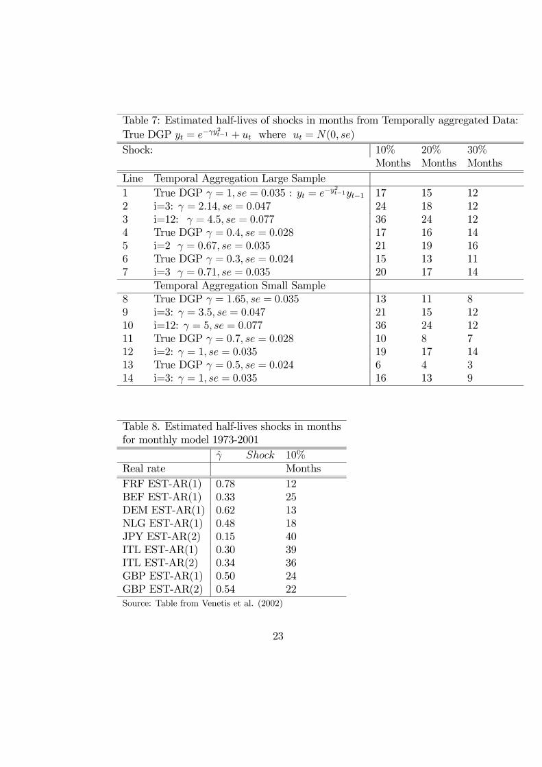
Table 7: Estimated half-lives of shocks in months from Temporally aggregated Data:True DGP yt = e−γy

2t−1 + ut where ut = N(0, se)

Shock: 10% 20% 30%Months Months Months

Line Temporal Aggregation Large Sample1 True DGP γ = 1, se = 0.035 : yt = e−y

2t−1yt−1 17 15 12

2 i=3: γ = 2.14, se = 0.047 24 18 123 i=12: γ = 4.5, se = 0.077 36 24 124 True DGP γ = 0.4, se = 0.028 17 16 145 i=2 γ = 0.67, se = 0.035 21 19 166 True DGP γ = 0.3, se = 0.024 15 13 117 i=3 γ = 0.71, se = 0.035 20 17 14

Temporal Aggregation Small Sample8 True DGP γ = 1.65, se = 0.035 13 11 89 i=3: γ = 3.5, se = 0.047 21 15 1210 i=12: γ = 5, se = 0.077 36 24 1211 True DGP γ = 0.7, se = 0.028 10 8 712 i=2: γ = 1, se = 0.035 19 17 1413 True DGP γ = 0.5, se = 0.024 6 4 314 i=3: γ = 1, se = 0.035 16 13 9

Table 8. Estimated half-lives shocks in monthsfor monthly model 1973-2001

γ̂ Shock 10%Real rate MonthsFRF EST-AR(1) 0.78 12BEF EST-AR(1) 0.33 25DEM EST-AR(1) 0.62 13NLG EST-AR(1) 0.48 18JPY EST-AR(2) 0.15 40ITL EST-AR(1) 0.30 39ITL EST-AR(2) 0.34 36GBP EST-AR(1) 0.50 24GBP EST-AR(2) 0.54 22Source: Table from Venetis et al. (2002)

23

Table 9. Estimated half-lives shocks in monthsfor quarterly model. 1973.I-1998.IV

γ̂ Shock 10%Real rate MonthsFRF EST-AR(2) 0.86 36DM EST-AR(2) 0.79 36CA EST-AR(2) 0.71 40IT EST-AR(2) 0.91 36JP EST-AR(2) 0.73 40SW EST-AR(2) 0.72 40GBP EST-AR(2) 1.07 36Source: Table from Kilian and Taylor (2003)

Table 10. Estimated half-lives shocks in monthsfor annual model

γ̂ Shock 10%Real rate MonthsFRF EST-AR(2) 1802-1992 4.04 36GBP EST-AR(2) 1792-1992 2.44 48DM EST-AR(2) 1794-1913 2.52 48

24

10.50-0.5-1

0.5

0.25

0

-0.25

-0.5

x

y

x

y

Deterministic plot of ∆ y (vertical axis), 1ty − (horizontal axis) from ESTAR with γ = 0.8.