
Tempered Particle Filtering - Yale University
75
Tempered Particle Filtering Edward Herbst Federal Reserve Board Frank Schorfheide * University of Pennsylvania PIER, CEPR, NBER July 21, 2017 Abstract The accuracy of particle filters for nonlinear state-space models crucially depends on the proposal distribution that mutates time t - 1 particle values into time t values. In the widely-used bootstrap particle filter, this distribution is generated by the state- transition equation. While straightforward to implement, the practical performance is often poor. We develop a self-tuning particle filter in which the proposal distribution is constructed adaptively through a sequence of Monte Carlo steps. Intuitively, we start from a measurement error distribution with an inflated variance, and then gradually reduce the variance to its nominal level in a sequence of tempering steps. We show that the filter generates an unbiased and consistent approximation of the likelihood function. Holding the run time fixed, our filter is substantially more accurate in two DSGE model applications than the bootstrap particle filter. JEL CLASSIFICATION: C11, C15, E10 KEY WORDS: Bayesian analysis, DSGE models, nonlinear filtering, Monte Carlo methods * Correspondence: E. Herbst: Board of Governors of the Federal Reserve System, 20th Street and Con- stitution Avenue N.W., Washington, D.C. 20551. Email: [email protected]. F. Schorfheide: Depart- ment of Economics, 3718 Locust Walk, University of Pennsylvania, Philadelphia, PA 19104-6297. We thank Sylvia Kaufmann (guest editor), three anonymous referees, Drew Creal, Andras Fulop, Juan Rubio-Ramirez, and participants at various seminars and conferences for helpful comments. Email: [email protected]. Schorfheide gratefully acknowledges financial support from the National Science Foundation under the grant SES 1424843. The views expressed in this paper are those of the authors and do not necessarily reflect the views of the Board of Governors or the Federal Reserve System.
Transcript of Tempered Particle Filtering - Yale University

Tempered Particle Filtering
Edward Herbst
Federal Reserve Board
Frank Schorfheide∗
University of Pennsylvania
PIER, CEPR, NBER
July 21, 2017
Abstract
The accuracy of particle filters for nonlinear state-space models crucially depends
on the proposal distribution that mutates time t− 1 particle values into time t values.
In the widely-used bootstrap particle filter, this distribution is generated by the state-
transition equation. While straightforward to implement, the practical performance is
often poor. We develop a self-tuning particle filter in which the proposal distribution is
constructed adaptively through a sequence of Monte Carlo steps. Intuitively, we start
from a measurement error distribution with an inflated variance, and then gradually
reduce the variance to its nominal level in a sequence of tempering steps. We show
that the filter generates an unbiased and consistent approximation of the likelihood
function. Holding the run time fixed, our filter is substantially more accurate in two
DSGE model applications than the bootstrap particle filter.
JEL CLASSIFICATION: C11, C15, E10
KEY WORDS: Bayesian analysis, DSGE models, nonlinear filtering, Monte Carlo methods
∗Correspondence: E. Herbst: Board of Governors of the Federal Reserve System, 20th Street and Con-
stitution Avenue N.W., Washington, D.C. 20551. Email: [email protected]. F. Schorfheide: Depart-
ment of Economics, 3718 Locust Walk, University of Pennsylvania, Philadelphia, PA 19104-6297. We thank
Sylvia Kaufmann (guest editor), three anonymous referees, Drew Creal, Andras Fulop, Juan Rubio-Ramirez,
and participants at various seminars and conferences for helpful comments. Email: [email protected].
Schorfheide gratefully acknowledges financial support from the National Science Foundation under the grant
SES 1424843. The views expressed in this paper are those of the authors and do not necessarily reflect the
views of the Board of Governors or the Federal Reserve System.

1
1 Introduction
Estimated dynamic stochastic general equilibrium (DSGE) models are now widely used by
academics to conduct empirical research in macroeconomics as well as by central banks to
interpret the current state of the economy, to analyze the impact of changes in monetary or
fiscal policies, and to generate predictions for macroeconomic aggregates. In most applica-
tions, the estimation uses Bayesian techniques, which require the evaluation of the likelihood
function of the DSGE model. If the model is solved with a (log)linear approximation and
driven by Gaussian shocks, then the likelihood evaluation can be efficiently implemented
with the Kalman filter. If, however, the DSGE model is solved nonlinearly, the resulting
state-space representation is nonlinear and the Kalman filter can no longer be used.
Fernandez-Villaverde and Rubio-Ramırez (2007) proposed using a particle filter to eval-
uate the likelihood function of a nonlinear DSGE model, and many other papers have since
followed this approach. However, configuring the particle filter so that it generates an ac-
curate approximation of the likelihood function remains a key challenge. The contribution
of this paper is to develop a self-tuning tempered particle filter that in our applications is
substantially more accurate than the widely-used bootstrap particle filter.
Our starting point is the state-space representation of a potentially nonlinear DSGE
model given by a measurement equation and a state-transition equation:
yt = Ψ(st; θ) + ut, ut ∼ N(0,Σu(θ)
)(1)
st = Φ(st−1, εt; θ), εt ∼ Fε(·; θ).
The functions Ψ(st; θ) and Φ(st−1, εt; θ) are generated numerically when solving the DSGE
model. Here yt is a ny× 1 vector of observables, ut is a ny× 1 vector of normally distributed
measurement errors, and st is an ns × 1 vector of hidden states.1 To obtain the likelihood
increments p(yt+1|Y1:t, θ), where Y1:t = {y1, . . . , yt}, it is necessary to integrate out the latent
states:
p(yt+1|Y1:t, θ) =
∫ ∫p(yt+1|st+1, θ)p(st+1|st, θ)p(st|Y1:t, θ)dst+1dst, (2)
which can be done recursively with a filter.
1In principle both Ψ(·) and Φ(·) could depend on the time period t in a deterministic manner. We omitthis dependency in our notation. The ut’s do not literally have to be measurement errors. They couldalso be innovations to fundamentals. All we require is a non-degenerate distribution of yt|st with a scalablecovariance matrix.
2
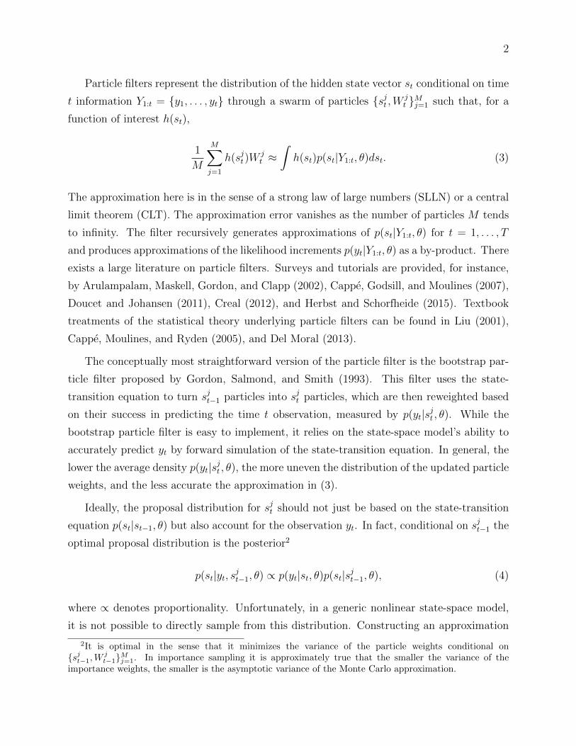
Particle filters represent the distribution of the hidden state vector st conditional on time
t information Y1:t = {y1, . . . , yt} through a swarm of particles {sjt ,W jt }Mj=1 such that, for a
function of interest h(st),
1
M
M∑j=1
h(sjt)Wjt ≈
∫h(st)p(st|Y1:t, θ)dst. (3)
The approximation here is in the sense of a strong law of large numbers (SLLN) or a central
limit theorem (CLT). The approximation error vanishes as the number of particles M tends
to infinity. The filter recursively generates approximations of p(st|Y1:t, θ) for t = 1, . . . , T
and produces approximations of the likelihood increments p(yt|Y1:t, θ) as a by-product. There
exists a large literature on particle filters. Surveys and tutorials are provided, for instance,
by Arulampalam, Maskell, Gordon, and Clapp (2002), Cappe, Godsill, and Moulines (2007),
Doucet and Johansen (2011), Creal (2012), and Herbst and Schorfheide (2015). Textbook
treatments of the statistical theory underlying particle filters can be found in Liu (2001),
Cappe, Moulines, and Ryden (2005), and Del Moral (2013).
The conceptually most straightforward version of the particle filter is the bootstrap par-
ticle filter proposed by Gordon, Salmond, and Smith (1993). This filter uses the state-
transition equation to turn sjt−1 particles into sjt particles, which are then reweighted based
on their success in predicting the time t observation, measured by p(yt|sjt , θ). While the
bootstrap particle filter is easy to implement, it relies on the state-space model’s ability to
accurately predict yt by forward simulation of the state-transition equation. In general, the
lower the average density p(yt|sjt , θ), the more uneven the distribution of the updated particle
weights, and the less accurate the approximation in (3).
Ideally, the proposal distribution for sjt should not just be based on the state-transition
equation p(st|st−1, θ) but also account for the observation yt. In fact, conditional on sjt−1 the
optimal proposal distribution is the posterior2
p(st|yt, sjt−1, θ) ∝ p(yt|st, θ)p(st|sjt−1, θ), (4)
where ∝ denotes proportionality. Unfortunately, in a generic nonlinear state-space model,
it is not possible to directly sample from this distribution. Constructing an approximation
2It is optimal in the sense that it minimizes the variance of the particle weights conditional on{sjt−1,W
jt−1}Mj=1. In importance sampling it is approximately true that the smaller the variance of the
importance weights, the smaller is the asymptotic variance of the Monte Carlo approximation.

3
for p(st|yt, sjt−1, θ) in a generic state-space model typically involves tedious model-specific
calculations that have to be executed by the user of the algorithm prior to its implementa-
tion.3 The innovation in this paper is to generate this approximation in a sequence of Monte
Carlo steps. The basic idea goes back to Godsill and Clapp (2001). Our starting point is
the observation that the larger the measurement error variance, the more accurate the filter
becomes, because holding everything else constant, the variance of the particle weights de-
creases. Building on this insight, in each period t, we generate sjt by forward simulation but
then update the particle weights based on a density p1(yt|st, θ) with an inflated measurement
error variance. In a sequence of tempering iterations we reduce this inflated measurement
error variance to its nominal level. These iterations mimic a sequential Monte Carlo (SMC)
algorithm designed for a static parameter. Such algorithms have been successfully used to
approximate posterior distributions for parameters of econometric models.4
We show that our proposed tempered particle filter produces a valid approximation of the
likelihood function and substantially reduces the Monte Carlo error relative to the bootstrap
particle filter, even after controlling for computational time. Our algorithm can be embedded
into particle Markov chain Monte Carlo (MCMC) algorithms that replace the true likelihood
by a particle-filter approximation; see, for instance, Fernandez-Villaverde and Rubio-Ramırez
(2007) for DSGE model applications and Andrieu, Doucet, and Holenstein (2010) for the
underlying statistical theory.
The idea of adding tempering steps to the particle filter dates back to Godsill and Clapp
(2001), but it has not been used in the DSGE model literature. Contemporaneously with our
paper, Johansen (2016) developed a particle filter that involves tempering iterations to track
p(st, st−1, . . . , st−L|Y1:t). While his algorithm allows for the mutation of particles representing
blocks of lagged states, no clear guidance is provided on how the algorithm should be tailored
in a specific application and whether the additional computational cost of mutating lagged
states is compensated by improvements in the accuracy of the likelihood approximation.
Moreover, the paper does not contain any theoretical results and the numerical illustration
is restricted to a univariate model rather than DSGE models with multidimensional state
spaces. In addition, in each time period t we are choosing the tempering schedule adaptively,
3Attempts include approximations based on the one-step Kalman filter updating formula applied to alinearized version of the DSGE model. Alternatively, one could use the updating step of an approximatefilter, e.g., the ones developed by Andreasen (2013) or Kollmann (2015).
4Chopin (2002) first showed how to use sequential Monte Carlo methods to conduct inference on aparameter that does not evolve over time. Applications to the estimation of DSGE model parametershave been considered in Creal (2007) and Herbst and Schorfheide (2014). Durham and Geweke (2014) andBognanni and Herbst (2015) provide applications to the estimation of other econometric time-series models.

4
building on work by Jasra, Stephens, Doucet, and Tsagaris (2011), Del Moral, Doucet,
and Jasra (2012), Schafer and Chopin (2013), Geweke and Frischknecht (2014), and Zhou,
Johansen, and Aston (2015).
There are essentially two methods of establishing theoretical properties of SMC approx-
imations. On the one hand, Del Moral (2004) and Del Moral (2013) use high-level random
field theory to establish theoretical properties of SMC methods through the lens of the
Feynman-Kac formula and its role in stochastic differential equations. While mathemati-
cally elegant, the approach relies on theory that is unfamiliar to most econometricians. On
the other hand, Chopin (2004) proves a CLT for SMC approximations recursively, using fa-
miliar (to econometricians) CLTs for non-identically and independently distributed random
variables. In a similar fashion, Pitt, Silva, Giordani, and Kohn (2012) show how one can
prove the unbiasedness of particle filter approximation without making use of the Feynman-
Kac formula. We follow this second route and show how the arguments in Chopin (2004)
and Pitt, Silva, Giordani, and Kohn (2012) can be extended to account for the tempering
iterations used in our algorithm. While the theoretical results in our paper are restricted
to a non-adaptive version of the filter, theoretical results for adaptive SMC algorithms have
recently been obtained by Beskos, Jasra, Kantas, and Thiery (2014).
The remainder of the paper is organized as follows. The proposed tempered particle
filter is presented in Section 2. We provide a SLLN for the particle filter approximation of
the likelihood function in Section 3 and show that the approximation is unbiased. Here we
are focusing on a version of the filter that is non-adaptive. The filter is applied to a small-
scale New Keynesian DSGE model and the Smets-Wouters model in Section 4 and Section 5
concludes. Theoretical derivations, computational details, DSGE model descriptions, and
data sources are relegated to the Online Appendix. To simplify the notation, we often drop
θ from the conditioning set of densities p(·|·).
2 The Tempered Particle Filter
A key determinant of the accuracy of a particle filter is the distribution of the normalized
weights
W jt =
wjtWjt−1
1M
∑Mj=1 w
jtW
jt−1
,

5
where W jt−1 is the (normalized) weight associated with the jth particle at time t − 1, wjt is
the incremental weight after observing yt, and W jt is the normalized weight accounting for
this new observation.5 For the bootstrap particle filter, the incremental weight is simply the
likelihood of observing yt given the jth particle, p(yt|sjt). It is approximately true that, all
else equal, the larger the variance of W jt ’s, the less accurate the Monte Carlo approximations
generated by the particle filter.
One can show that, as the measurement error variance increases, the variance of the
particle weights {Wt}Mj=1 decreases. Let Σu/φn, 0 < φn ≤ 1 be an inflated measurement
error covariance matrix. Then,
pn(yt|st) ∝ exp
{−1
2φn(yt −Ψ(st))
′Σ−1u (yt −Ψ(st))
}. (5)
Assuming that a resampling step equalized the particle weights W jt−1 = 1, it is straightfor-
ward to verify that
limφn−→0
W jt =
pn(yt|sjt)1M
∑Mj=1 pn(yt|sjt)
= 1. (6)
Thus, in the limit, the variance of the particle weights is equal to zero. With a bit more
algebra, it can be verified that the variance of the particle weights monotonically decreases as
φn −→ 0 (see the Online Appendix for details). We use this insight to construct a tempered
particle filter in which we generate proposed particle values sjt sequentially, by reducing the
measurement error variance from an inflated initial level Σu/φ1 to the nominal level Σu using
a sequence of scale factors 0 < φ1 < φ2 < . . . < φNφ = 1. The reduction of the measurement
error variance is achieved by a sequence of Monte Carlo steps that we borrow from the
literature of SMC approximations for posterior moments of static parameters.
By construction, pNφ(yt|st) = p(yt|st). Based on pn(yt|st), we can define the bridge
distributions
pn(st|yt, st−1) ∝ pn(yt|st)p(st|st−1). (7)
Integrating out st−1 under the distribution p(st−1|Y1:t−1) yields the bridge posterior density
5In the notation developed subsequently, the tilde on W jt indicates that this is the weight associated with
particle j before any resampling of the particles.

6
for st conditional on the observables:
pn(st|Y1:t) =
∫pn(st|yt, st−1)p(st−1|Y1:t−1)dst−1. (8)
In the remainder of this section, we describe the proposed tempered particle filter. Section 2.1
presents the main algorithm that iterates over periods t = 1, . . . , T to approximate the
likelihood increments p(yt|Y1:t−1) and the filtered states p(st|Y1:t). In Section 2.2, we focus
on the novel component of our algorithm, which in every period t uses Nφ steps to reduce the
measurement error variance from Σu/φ1 to Σu. We provide specific guidance for practitioners
on tuning the tempered particle filter in Section 2.3. Finally, in Section 2.4 we briefly discuss
the relationship between the tempered and the conditionally-optimal particle filter.
2.1 The Main Iterations
The tempered particle filter has the same structure as the bootstrap particle filter. In
every period t, we draw innovations εt and use the state-transition equation to simulate the
state vector forward; we update the particle weights; and we resample the particles. The
key difference is to start out with a fairly large measurement error variance, which is then
iteratively reduced to the nominal level Σu. During this tempering, we adjust the innovations
to the state-transition equation as well as the particle weights.
The tempering sequence and the number of tempering stages may differ for every time
period t. Thus, a concise notation takes the form
φ1,t < φ2,t < . . . < φNφt
= 1 instead of φ1 < φ2 < . . . < φNφ = 1.
Starting from the distribution p(st−1|Y1:t−1) and using a sequence of tempering iterations,
our filter tracks the bridge distributions pn(st|Y1:t) defined in (8) for n = 1, . . . , Nφt . As our
filter cycles through the tempering iterations and mutates the particle values sj,nt , it keeps
the particle values sj,Nφ
t−1
t−1 unchanged. The pairs (sj,nt , sj,Nφ
t−1
t−1 ) with their associated particle
weights approximate the distributions
pn(st, st−1|Y1:t) = pn(st|st−1, Y1:t)p(st−1|Y1:t) for n = 1, . . . , Nφt .
Because it is convenient for the implementation of the mutation steps, we will include εt
in the vector of particle values and track the triplet (st, εt, st−1) with the understanding

7
that this triplet always satisfies the state-transition equation st = Φ(st−1, εt). Algorithm 1
summarizes the iterations over periods t = 1, . . . , T . For now, it is assumed that the initial
scalings of the measurement error variances φ1,t, t = 1, . . . , T , are given. We use h(st, st−1)
to denote a generic integrable function of interest.
Algorithm 1 (Tempered Particle Filter)
1. Period t = 0 Initialization. Let Nφ0 = 1. Draw the initial particles from the distri-
bution sj0iid∼ p(s0), j = 1, . . . ,M . Let s
j,Nφ0
0 = sj0 and Wj,Nφ
00 = 1.
2. Period t Iterations. For t = 1, . . . , T :
(a) Particle Initialization.
i. Starting from {sj,Nφt−1
t−1 ,Wj,Nφ
t−1
t−1 }, generate εj,1t ∼ Fε(·) and define
sj,1t = Φ(sj,Nφ
t−1
t−1 , εj,1t ).
ii. Compute the incremental weights:
wj,1t = p1(yt|sj,1t ) ∝ exp
{− 1
2φ1,t
(yt −Ψ(sj,1t )
)′Σ−1u
(yt −Ψ(sj,1t )
)}. (9)
iii. Normalize the incremental weights:
W j,1t =
wj,1t Wj,Nφ
t−1
t−1
1M
∑Mj=1 w
j,1t W
j,Nφt−1
t−1
(10)
to obtain the particle swarm {sj,1t , εj,1t , sj,Nφ
t−1
t−1 , W j,1t }, which leads to
h1t =
1
M
M∑j=1
h(sj,1t , sj,Nφ
t−1
t−1 )W j,1t ≈
∫h(st, st−1)p1(st, st−1|Y1:t)dstdst−1. (11)
Moreover,
1
M
M∑j=1
wj,1t Wj,Nφ
t−1
t−1 ≈ p1(yt|Y1:t−1). (12)
iv. Resample the particles:
{sj,1t , εj,1t , sj,Nφ
t−1
t−1 , W j,1t } 7→ {sj,1t , εj,1t , s
j,Nφt−1
t−1 ,W j,1t },

8
to obtain the approximation
h1t =
1
M
M∑j=1
h(sj,1t , sj,Nφ
t−1
t−1 )W j,1t ≈
∫h(st, st−1)p1(st, st−1|Y1:t)dstdst−1. (13)
(b) Tempering Iterations: Execute Algorithm 2 (see next section) to
i. convert the particle swarm
{sj,1t , εj,1t , sj,Nφ
t−1
t−1 ,W j,1t } 7→ {sj,N
φt
t , εj,Nφ
tt , s
j,Nφt−1
t−1 ,Wj,Nφ
tt }
to approximate
hNφt
t =1
M
M∑j=1
h(sj,Nφ
tt , s
j,Nφt−1
t−1 )Wj,Nφ
tt (14)
≈∫h(st, st−1)p(st, st−1|Y1:t)dstdst−1;
ii. compute the approximation p(yt|Y1:t−1) of the likelihood increment.
3. Likelihood Approximation
p(Y1:T ) =T∏t=1
p(yt|Y1:t−1). � (15)
If one sets φ1,t = 1, Nφt = 1, and omits Step 2.(b) for all t, then Algorithm 1 is exactly
identical to the bootstrap particle filter: the sjt−1 particle values are simulated forward using
the state-transition equation; the weights are then updated based on how well the new state
sjt predicts the time t observations, measured by the predictive density p(yt|sjt); and finally
the particles are resampled using a standard resampling algorithm, such as multinominal
resampling, or systematic resampling.6 Once the resampling step has been executed, the
particle weights are equalized: W j,1t = 1 for j = 1, . . . ,M .
The drawback of the bootstrap particle filter is that the proposal distribution for the
innovation εjt ∼ Fε(·) is not adapted to the period t observation yt. This typically leads
to a large variance of wjt , which translates into inaccurate Monte Carlo approximations.
Taking the states {sjt−1}Mj=1 as given and assuming that a t−1 resampling step has equalized
6Detailed textbook treatments of resampling algorithms can be found in Liu (2001) and Cappe, Moulines,and Ryden (2005).

9
the particle weights, that is, W jt−1 = 1, the conditionally optimal choice for the proposal
distribution is p(εjt |sjt−1, yt). However, because of the nonlinearity in state-transition and
measurement equation, it is not possible to directly generate draws from this distribution.
Our algorithm sequentially adapts the proposal distribution for the innovations to the current
observation yt by raising φn from a small initial value to φNφ = 1. This is done in Step 2(b),
which is described in detail in Algorithm 2 in the next section.
2.2 Tempering the Measurement Error Variance
The idea of including tempering iterations into a particle filter dates back to Godsill and
Clapp (2001). These iterations build on Neal’s (1998) annealed importance sampling and
mimic the steps of SMC algorithms that have been developed for static parameters (e.g.,
Chopin (2002), Del Moral, Doucet, and Jasra (2006), Durham and Geweke (2014), and
Herbst and Schorfheide (2014, 2015)). SMC algorithms for static parameters generate draws
from a sequence of bridge posteriors pn(θ|Y ). These bridge posteriors can be generated
by tempering the likelihood function, i.e., pn(θ|Y ) ∝[p(Y |θ)
]φnp(θ), n = 1, . . . , Nφ with
φNφ = 1. At each iteration, the algorithm cycles through three stages: the particle weights
are updated in the correction step; the particles are being resampled and the particle weights
are equalized in the selection step; and the particle values are changed in the mutation step.
The analogue of[p(Y |θ)
]φnin our algorithm is pn(yt|st) given in (5), which reduces to p(yt|st)
for φn = 1. Algorithm 2 comprises of the correction, selection, and mutation steps. Note
that the sequence φn,t, n = 1, . . . , Nφt , and the number of stages, Nφ
t , is an output of the
algorithm that is determined in Step 1(a)iii. in conjunction with the termination condition
φn,t = 1 of the do-loop. Thus, the filter is adaptive with respect to the tempering schedule.
Algorithm 2 (Tempering Iterations) This algorithm receives as input the particle swarm
{sj,1t , εj,1t , sj,Nφ
t−1
t−1 ,W j,1t } and returns as output the particle swarm {sj,N
φt
t , εj,Nφ
tt , s
j,Nφt−1
t−1 ,Wj,Nφ
tt }
and the likelihood increment pNφt(yt|Y1:t−1). Set n = 1 and Nφ
t = 1.
1. Do until φn,t = 1:
(a) Correction: Let n = n+ 1. Then,

10
i. for j = 1, . . . ,M and given φn−1,t define the incremental weight function
wj,nt (φn) =pn(yt|sj,n−1
t )
pn−1(yt|sj,n−1t )
(16)
=
(φn
φn−1,t
)ny/2exp
{− 1
2
[yt −Ψ(sj,n−1
t )]′
×(φn − φn−1,t)Σ−1u
[yt −Ψ(sj,n−1
t )]}.
ii. Define the normalized weights
W j,nt (φn) =
wj,nt (φn)W j,n−1t
1M
∑Mj=1 w
j,nt (φn)W j,n−1
t
, (17)
(W j,n−1t = 1 because the resampling step was executed in iteration n−1), and
the inefficiency ratio
InEff(φn) =1
M
M∑j=1
(W j,nt (φn)
)2. (18)
iii. If InEff(1) ≤ r∗
let φn,t = 1, Nφt = n, and W j,n
t = W j,nt (1) (terminate do-loop after
iteration n);
else
let φn,t be the solution to InEff(φn,t) = r∗, W j,nt = W j,n
t (φn,t).
iv. The particle swarm {sj,n−1t , εj,n−1
t , sj,Nφ
t−1
t−1 , W j,nt } approximates
hnt =1
M
M∑j=1
h(sj,n−1t , s
j,Nφt−1
t−1 )W j,nt (19)
≈∫h(st, st−1)pn(st, st−1|Y1:t)dstdst−1.
(b) Selection: Resample the particles:
{sj,n−1t , εj,n−1
t , sj,Nφ
t−1
t−1 , W j,nt } 7→ {sj,nt , εj,nt , s
j,Nφt−1
t−1 ,W j,nt },
which leads to W j,nt = 1 for j = 1, . . . ,M . Keep track of the correct ancestry infor-
mation such that sj,nt = Φ(sj,Nφ
t−1
t−1 , εj,nt ) for each j. This leads to the approximation

11
hnt =1
M
M∑j=1
h(sj,nt , sj,Nφ
t−1
t−1 )W j,nt ≈
∫h(st, st−1)pn(st, st−1|Y1:t)dstdst−1. (20)
(c) Mutation: Use a Markov transition kernel Kn(st|st; st−1) with the invariance
property
pn(st|yt, st−1) =
∫Kn(st|st; st−1)pn(st|yt, st−1)dst (21)
to mutate the particle values (see Algorithm 3 for an implementation). This leads
to the particle swarm {sj,nt , εj,nt , sj,Nφ
t−1
t−1 ,W j,nt }, which approximates
hnt =1
M
M∑j=1
h(sj,nt , sj,Nφ
t−1
t−1 )W j,nt ≈
∫h(st, st−1)pn(st, st−1|Y1:t)dstdst−1. (22)
2. Approximate the likelihood increment:
p(yt|Y1:t−1) = pNφt(yt|Y1:t−1) =
Nφt∏
n=1
(1
M
M∑j=1
wj,nt W j,n−1t
)(23)
with the understanding that W j,0t = W
j,Nφt−1
t−1 . �
Correction. The correction step adapts the stage n − 1 particle swarm to the reduced
measurement error variance in stage n by reweighting the particles. The incremental weights
in (16) capture the change in the measurement error variance from Σu/φn−1,t to Σu/φn and
yield an importance sampling approximation of pn(st|Y1:t) based on the stage n− 1 particle
values. We choose φn,t to achieve a targeted inefficiency ratio r∗ > 1. This approach of
adaptively choosing the tempering schedule has been used in the SMC literature by Jasra,
Stephens, Doucet, and Tsagaris (2011), Del Moral, Doucet, and Jasra (2012), Schafer and
Chopin (2013), and Zhou, Johansen, and Aston (2015). It also has proven useful in the
context of global optimization of nonlinear functions; see Geweke and Frischknecht (2014).
To relate the inefficiency ratio to φn, we begin by defining
ej,t =1
2(yt −Ψ(sj,n−1
t ))′Σ−1u (yt −Ψ(sj,n−1
t )).

12
Assuming that the particles were resampled in iteration n− 1 and W j,n−1t = 1, we can then
express the inefficiency ratio as
InEff(φn) =1
M
M∑j=1
(W j,nt (φn)
)2=
1M
∑Mj=1 exp[−2(φn − φn−1,t)ej,t](
1M
∑Mj=1 exp[−(φn − φn−1,t)ej,t]
)2 . (24)
For φn = φn−1,t the inefficiency ratio is InEff(φn) = 1 < r∗. We show in the Online Ap-
pendix that the function is monotonically increasing on the interval [φn−1,t, 1], which is the
justification for Step 1(a)iii of Algorithm 3. Thus, we are raising φn as closely to one as we
can without exceeding a user-defined bound on the variance of the particle weights. We use
the same approach to set the initial scaling factor φ1 in Algorithm 1.
Selection. The selection step is executed in every iteration n to ensure that we can find a
unique φn,t based on the function InEff(φn) in (24) in the correction step. Thus, W j,nt = 1
and in principle we could drop the weights from the formulas.
Mutation. In the mutation step, we are using a Markov transition kernel to change the
particle values from (sj,nt , εj,nt ) to (sj,nt , εj,nt ), maintaining an approximation of pn(st, st−1|Y1:t).
It can be implemented with a random walk Metropolis-Hastings (RWMH) algorithm; see
Algorithm 3 below. In the absence of the mutation step, the initial particle values (sj,1t , εj,1t )
would never change and we would essentially reproduce the bootstrap particle filter by
computing p(yt|sjt) as the limit of a sequence of measurement error covariance matrices that
converges to Σu. Unlike in the algorithm proposed by Johansen (2016), we do not mutate
the particle values sj,Nφ
t−lt−l , l = 1, . . . , L. The advantage is that the state vector that we are
mutating has a smaller dimension, which tends to increase the probability that a particle
value changes during the mutation step. Thus, our algorithm should be able to attain a
desired probability of mutating the particle values with fewer steps of the RWMH algorithm
and therefore be faster. A potential disadvantage is that we are not adapting as well to the
joint distribution pn(st, st−1, . . . , st−L|Y1:t).
Algorithm 3 (RWMH Mutation Step) This algorithm receives as input the particle swarm
{sj,nt , εj,nt , sj,Nφ
t−1
t−1 ,W j,nt } and returns as output the particle swarm {sj,nt , εj,nt , s
j,Nφt−1
t−1 ,W j,nt }.
1. Execute NMH Metropolis-Hastings Steps for Each Particle: For j = 1, . . .M :
(a) Set εj,n,0t = εj,nt . Then, for l = 1, . . . , NMH :
i. Generate a proposed innovation: ejt ∼ N(εj,n,l−1t , c2
nInε).

13
ii. Compute the acceptance rate:
α(ejt |εj,n,l−1t ) = min
1,pn(yt|ejt , s
j,Nφt−1
t−1 )pε(ejt)
pn(yt|εj,n,l−1t , s
j,Nφt−1
t−1 )pε(εj,n,l−1t )
.
iii. Update particle values:
εj,n,lt =
{ejt with prob. α(ejt |εj,n,l−1
t )
εj,n,l−1t with prob. 1− α(ejt |εj,n,l−1
t )
(b) Define εj,nt = εj,n,NMH
t and sj,nt = Φ(sj,Nφ
t−1
t−1 , εj,nt ). �
As the covariance matrix for the proposal distribution in the RWMH algorithm we use
the identity matrix Inε scaled by cn.7 We set cn adaptively to achieve a desired acceptance
rate. We compute the average empirical rejection rate Rn−1(cn−1) across the NMH RWMH
steps of the mutation phase in iteration n− 1. We set c1 = c∗ and let
cn = cn−1f(1− Rn−1(cn−1)
), f(x) = 0.95 + 0.10
e20(x−0.40)
1 + e20(x−0.40), n ≥ 2. (25)
Thus, we increase (decrease )the scaling factor by 5 percent if the acceptance rate is well above
(below) 0.40. For acceptance rates near 0.40, the increase (or decrease) of cn is attenuated
by the logistic component of f(x). In our empirical applications, the performance of the
filter was robust to variations of the rule.
2.3 Tuning of the Algorithm
In order to run Algorithm 3, the user has to specify the number of particles M , the initial
measurement error precision scalings φ1,t in Algorithm 1, the targeted inefficiency ratio
r∗, the initial scaling of the proposal covariance matrix c∗, and the number of Metropolis-
Hastings steps NMH . In principle, the user can also adjust the target acceptance rate (and
potentially the speed of adjustment) in (25). Each of these tuning parameters affects the
statistical properties of the filter, and can potentially affect the computational cost associated
with the filter. We now discuss some issues in selecting each of these parameters.
7Herbst and Schorfheide (2014) use the particle approximation of the posterior covariance matrix fromthe selection step to specify the stage-n proposal covariance matrix. In the tempered particle filter, the costof computing this object tends to outweigh the gains from adapation, so we instead use the identity matrix.

14
The selection of M is an issue for any particle filter. A higher M is associated with
a more precise approximation at the cost of a longer run time of the filter. In practice,
this is usually done through experimentation. If the particle filter is embedded in a MCMC
algorithm, a heuristic suggested by Pitt, Silva, Giordani, and Kohn (2012), is to increase M
until the standard deviation of the filter’s log likelihood estimate at some parameter value is
less than one. Particle filter approximations typically satisfy a CLT according to which the
variance is proportional to 1/M .
The initial measurement error precisions φ1,t can either be user-specified or determined
adaptively by targeting a desired variance of particle weights as in Step 1(a)iii of Algorithm 2.
The targeted inefficiency ratio, r∗ ∈ (1,∞) controls the targeted degree of “unevenness” of
the distribution of particle weights that pins down the particular φn,t sequences. If r∗ is close
to 1, loosely speaking, φn,t will be “close” to φn−1,t and generally there will be many stages
(Nφt will be large.) In contrast, if r∗ is very large, bridge distributions can be very different,
and in general Nφt will be small. In the limit, as r∗ −→ ∞, the algorithm converges to the
resample-move variant of the bootstrap particle filter, where Nφt = 1 for all t. The particles
are mutated at each time t, but there are no intermediate bridge distributions.
A low r∗ delivers weighted particles with low variance, which all else equal are associated
with more precise Monte Carlo estimates. Of course, a low r∗ is also associated with many
bridge distributions, which increases the run time of the filter. At some point increasing
the number of tempering iterations further could in principle result in less precise estimates
because of the variability induced by the additional resampling and mutation steps. In
practice, we don’t find this to be an issue, and so r∗ works as a complement to M , with
both having a trade-off between statistical precision and computational cost. In Section 4
we examine the effects of different choices of M and r∗ in two DSGE models.
The other two tuning parameters, namely, the initial scaling of the proposal covariance
matrix c∗ and the number of RWMH steps NMH , are less important. If there are many
bridge distributions, the influence of the initial scaling factor c∗ is diminished because it is
adjusted in each subsequent iteration. While many intermediate RWMH steps help to ensure
that the particles are both diverse and well-adapted to any given bridge distribution, often
this effect can be achieved by choosing a lower r∗. Of course, this is not to say that c∗ and
NMH do not affect the variance of the Monte Carlo estimates. In any particular application,
experimentation with these parameters may enhance the performance of the algorithm.
Finally, we could replace the draws of εj,1t from the innovation distribution Fε(·) in
15
Step 2(a)i of Algorithm 1 with draws from a tailored distribution with density g1t (ε
j,1t |s
j,Nφt−1
t−1 )
and then adjust the incremental weight ωj,1t by the ratio pε(εj,1t )/g1
t (εj,1t |s
j,Nφt−1
t−1 ), as it is done
in the generalized version of the particle filter. Here the gt(·) density might be constructed
based on a linearized version of the DSGE model or be obtained through the updating steps
of a conventional nonlinear filter, such as an extended Kalman filter, unscented Kalman fil-
ter, or a Gaussian quadrature filter; see Herbst and Schorfheide (2015). Thus, the proposed
tempering steps can be used either to relieve the user from the burden of having to construct
a g1t (ε
j,1t |s
j,Nφt−1
t−1 ) in the first place, or it could be used to improve upon the accuracy obtained
with a readily available g1t (ε
j,1t |s
j,Nφt−1
t−1 ).
2.4 Relationship to Conditionally-Optimal Particle Filter
We mentioned in the introduction that conditional on the sjt−1 particles it is optimal to
generate draws from the proposal distribution p(st|yt, st−1) given in (4). The tempered
particle filter generates a sequence of approximations pn(st, st−1|yt, Y1:t−1) that converge to
p(st, st−1|yt, Y1:t−1) as n −→ Nφ. This raises the question to what extent this filter can
achieve conditional optimality. Because p(st|yt, st−1) and pn(st, st−1|yt, Y1:t−1) are not the
same objects, we provide a comparison of the two approaches by embedding the conditionally-
optimal proposal distribution into Algorithm 1.
Suppose in Step 2(a)i we draw sj,1t,∗ (we are using the ∗ subscript to indicate draws and
weights associated with the conditionally-optimal proposal) from
p1(st|yt, sj,Nφ
t−1
t−1 ) ∝ p1(yt|st)p(st|sj,Nφ
t−1
t−1 ), (26)
where p1(yt|st) is based on scaling the precision of the measurement errors by φ1,t.8 The
incremental weights for sj,1t,∗ are given by
wj,1t,∗ = p1(yt|sj,1t,∗)p(sj,1t,∗|s
j,Nφt−1
t−1 )
p1(sj,1t,∗|yt, sj,Nφ
t−1
t−1 )= p1(yt|s
j,Nφt−1
t−1 ). (27)
For every choice φ1 of the measurement error precision, the variance of the wj,1t,∗ weights is
smaller than the variance of the weights wj,1t obtained under the bootstrap proposal, because
8If one can sample from the conditionally-optimal proposal for φn,t = 1, then it is reasonable to assumethat one can sample from this density for 0 < φn,t ≤ 1. This is certainly true for normally distributedmeasurement errors.

16
the conditionally-optimal proposal is designed to minimize the variance of the particle weights
conditional on the swarm {sj,Nφt−1
t−1 ,Wj,Nφ
t−1
t−1 }. Moreover, we know from (24) that the variance
of the particle weights is an increasing function of φ1,t. Thus, if we choose φ1,t adaptively
according to Step 1(a)iii of Algorithm 2 by targeting a specific variance of the particle weights
(or a particular inefficiency ratio), then it has to be the case that the precision chosen under
the conditionally-optimal proposal, say φ∗1,t, is larger (and closer to one) than the precision
φ1,t chosen under the bootstrap proposal.
This leads to the following conclusions: (i) if the variance of the wj,1t,∗ is sufficiently small,
then φ∗1,t = 1 and the tempering iterations become obsolete. (ii) If the variance of the wj,1t,∗ is
large enough such that φ∗1,t < 1, then, because φ∗1,t ≥ φ1,t, the tempered particle filter with
the conditionally-optimal proposal distribution will be more accurate than the tempered
particle filter based on the bootstrap proposal. The former will either use fewer iterations
to bridge the discrepancy between p1(st, st−1|Y1:t) and p(st, st−1|Y1:t) or it will use the same
number of iterations with smaller gaps between pn−1(st, st−1|Y1:t) and pn(st, st−1|Y1:t).
The implementation of the conditionally-optimal particle filter is typically infeasible in
practice. Thus, the tempered particle filter is meant to be a feasible alternative that domi-
nates the widely-used bootstrap particle filter. However, the discussion emphasizes an impor-
tant point made at the end of Section 2.3: if a better proposal than p(st|sj,Nφ
t−1
t−1 ) is available,
then it should be used along with the tempering iterations.
3 Theoretical Properties of the Filter
We will now examine the asymptotic (with respect to the number of particles M) and finite
sample properties of the particle filter approximation of the likelihood function. Section 3.1
provides a SLLN, and Section 3.2 shows that the likelihood approximation is unbiased.
Detailed proofs are provided in the Online Appendix. Throughout this section, we will focus
on a version of the filter that is non-adaptive9, replacing Algorithm 2 by Algorithm 4 and
Algorithm 3 by Algorithm 5:
Algorithm 4 (Tempering Iterations – Non-Adaptive) This algorithm is identical to
Algorithm 2, with the exception that the tempering schedule {φn}Nφ
n=1 is pre-determined. The
9To simplify notation, we also assume that the tempering schedule is the same for all t. This assumptioncan be easily relaxed as long as the tempering schedule remains predetermined. Asymptotic results foradaptive SMC algorithms are available in the literature, e.g., Herbst and Schorfheide (2014) and Beskos,Jasra, Kantas, and Thiery (2014).

17
Do until φn,t = 1-loop is replaced by a For n = 1 to Nφ-loop and Step 1(a)iii is eliminated.
�
Algorithm 5 (RWMH Mutation Step – Non-Adaptive) This algorithm is identical
to Algorithm 3 with the exception that the sequence {cn}Nφ
n=1 is pre-determined. �
3.1 Asymptotic Properties
Under suitable regularity conditions, the Monte Carlo approximations generated by a particle
filter satisfy a SLLN and a CLT. Proofs for a generic particle filter are provided in Chopin
(2004). We will subsequently establish a SLLN for the tempered particle filter by modifying
the recursive proof developed by Chopin (2004) to account for the tempering iterations of
Algorithm 4. In this paper, we are primarily interested in establishing an almost-sure limit
for the Monte Carlo approximation of the likelihood function:
p(Y1:T ) =T∏t=1
p(yt|Y1:t−1)a.s.−→
T∏t=1
p1(yt|Y1:t−1)Nφ∏n=2
pn(yt|Y1:t−1)
pn−1(yt|Y1:t−1)
= p(Y1:T ). (28)
Here we used pNφ(yt|Y1:t−1) = p(yt|Y1:t−1). The limit is obtained by letting the number of
particles M −→∞. We assume that the length of the sample T is fixed. We use C <∞ to
denote a generic finite constant.
As a by-product, we also derive an almost-sure limit for Monte Carlo approximations of
moments of the filtered states:
hnt =1
M
M∑j=1
h(sj,nt , sj,Nφ
t−1 )W j,nt
a.s.−→∫ ∫
h(st, st−1)pn(st, st−1|Y1:t)dstdst−1, (29)
where
pn(st, st−1|Y1:t) =pn(yt|st)p(st|st−1)p(st−1|Y1:t−1)∫ ∫
pn(yt|st)p(st|st−1)p(st−1|Y1:t−1)dst−1dstdst−1
.
By integrating over st−1 we recover∫pn(st, st−1|Y1:t)dst−1 = pn(st|Y1:t),
where pn(st|Y1:t) was previously introduced in (8). For technical reasons that will be ex-
plained below, we consider expectations of generic functions h(st, st−1) that may vary with

18
both st and st−1.10 A special case is a function that is constant with respect to st−1. We
simply denote such a function by h(st).
To guarantee the almost-sure convergence, we need to impose some regularity conditions
on the functions h(st, st−1). We define the following classes of functions:
H1t =
{h(st, st−1)
∣∣∣∣ ∫ Ep(st|st−1)[|h(st, st−1)|]p(st−1|Y1:t−1)dst−1 <∞, (30)
∃δ > 0 s.t. fδ(st−1) = Ep(st|st−1)
[∣∣h(st, st−1)− Ep(st|st−1)[h(st, st−1)]∣∣1+δ
]< C,
g(st−1) = Ep(st|st−1)[h(st, st−1)] ∈ HNφ
t−1
}and for n = 2, . . . , Nφ:
Hnt =
{h(st, st−1)
∣∣∣∣h(st, st−1) ∈ Hn−1t , ∃δ > 0 s.t. (31)
fδ(st, st−1) = EKn(st|st;st−1)
[∣∣h(st, st−1)− EKn(st|st,st−1)[h(st, st−1)]∣∣1+δ
]< C,
g(st, st−1) = EKn(st|st;st−1)[h(st, st−1)] ∈ Hn−1t
}.
Here Ep(st|st−1)[·] and EKn(st|st,st−1)[·] are conditional expectations under the density p(st|st−1)
and the Markov transition kernel Kn(st|st; st−1). By definition, Hnt ⊆ Hn
t for n > n. The
classes Hnt are chosen such that the moment bounds that guarantee the almost sure con-
vergence of Monte Carlo averages of h(sj,nt , sj,Nφ
t−1 ) are satisfied. The key assumption here is
that there exists a uniform bound for the centered 1 + δ conditional moment of the function
h(st, st−1) under the state-transition density p(st|st−1) and the transition kernel of the muta-
tion step of Algorithm 5, Kn(st|st; st−1). This will allow us to apply a SLLN to the particles
generated by the forward simulation of the model and the mutation step in the tempering
iterations.
For the class H11 to be properly defined according to (30), we need to define HNφ
0 . Let
H0 = HNφ
0 and note that Ep(s1|s0)[h(s1, s0)] is a function of s0 only. Thus, we define
H0 =
{h(s0)
∣∣∣∣ ∫ |h(s0)|p(s0)ds0 <∞}. (32)
10Spoiler alert: we need the st−1 because the Markov transition kernel generated by Algorithm 4 (orAlgorithm 2) is invariant under the distribution pn(st|yt, st−1), which is conditioned on st−1, instead of thedistribution pn(st|Y1:t).

19
Under the assumption that the initial particles are generated by i.i.d. sampling from p(s0),
the integrability conditions ensure that we can apply Kolmogorov’s SLLN. Notice that any
bounded function |h(·)| < C is an element of Hnt for all t and n. Under the assumption that
the measurement errors have a multivariate normal distribution, the densities pn(yt|st) and
the density ratios pn(yt|st)/pn−1(yt|st) are bounded uniformly in st, which means that these
functions are elements of all Hnt .
By changing the definition of the classesHnt and requiring moments of order 2+δ to exist,
the subsequent theoretical results can be extended to a CLT following arguments in Chopin
(2004) and Herbst and Schorfheide (2014). The CLT provides a justification for computing
numerical standard errors from the variation of Monte Carlo approximations across multiple
independent runs of the filter.
3.1.1 Algorithm 1
To prove the convergence of the Monte Carlo approximations generated in Step 2(a) of
Algorithm 1, we can use well established arguments for the bootstrap particle filter, which we
adapt from the presentation in Herbst and Schorfheide (2015). We usea.s.−→ to denote almost-
sure convergence as M −→∞. The starting point is the following recursive assumption:
Assumption 1 The particle swarm {sj,Nφ
t−1 ,Wj,Nφ
t−1 } generated by the period t−1 iteration of
Algorithm 1 approximates:
hNφ
t−1 =1
M
M∑j=1
h(sj,Nφ
t−1 )W j,Nφ
t−1a.s.−→
∫h(st−1)p(st−1|Y1:t−1)dst−1 (33)
for functions h(st−1) ∈ HNφ
t−1.
In our statement of the recursive assumption, we only consider functions that vary with
st−1, which is why we write h(st−1) (instead of h(st−1, st−2)). As discussed previously, if the
filter is initialized by direct sampling from p(s0), then the recursive assumption is satisfied
for t = 1. We obtain the following convergence results:

20
Lemma 1 Suppose that Assumption 1 is satisfied. Then for h ∈ H1t :
h1t|t−1 =
1
M
M∑j=1
h(sj,1t , sj,Nφ
t−1 )W j,Nφ
t−1a.s.−→
∫ ∫h(st, st−1)p1(st, st−1|Y1:t−1)dstdst−1(34)
h1t =
1M
∑Mj=1 h(sj,1t , s
j,Nφ
t−1 )wj,1t Wj,Nφ
t−1
1M
∑Mj=1 w
j,1t W
j,Nφ
t−1
a.s.−→∫ ∫
h(st, st−1)p1(st, st−1|Y1:t)dstdst−1 (35)
h1t =
1
M
M∑j=1
h(sj,1t , sj,Nφ
t−1 )W j,1t
a.s.−→∫ ∫
h(st, st−1)p1(st, st−1|Y1:t)dstdst−1. (36)
Moreover,
p1(yt|Y1:t−1) =1
M
M∑j=1
wj,1t Wj,Nφ
t−1a.s.−→
∫p1(yt|st)p1(st|Y1:t−1)dst. (37)
3.1.2 Algorithm 4
The convergence results for the tempering iterations rely on the following recursive assump-
tion, which according to Lemma 1 is satisfied for n = 2.
Assumption 2 For n ≥ 2, the particle swarm {sj,n−1t , sj,N
φ
t−1 ,Wj,n−1t } generated by iteration
n− 1 of Algorithm 4 approximates:
hn−1t =
1
M
M∑j=1
h(sj,n−1t , sj,N
φ
t−1 )W j,n−1t
a.s.−→∫ ∫
h(st, st−1)pn−1(st, st−1|Y1:t)dstdst−1 (38)
for functions h ∈ Hn−1t .
The convergence results are stated in the following lemma:
Lemma 2 Suppose that Assumption 2 is satisfied. Then for n ≥ 2 and h ∈ Hn−1t :
hnt =1M
∑Mj=1 h(sj,n−1
t , sj,Nφ
t−1 )wj,nt W j,n−1t
1M
∑Mj=1 w
j,nt W j,n−1
t
(39)
a.s.−→∫ ∫
h(st, st−1)pn(st, st−1|Y1:t)dstdst−1
hnt =1
M
M∑j=1
h(sj,nt , sj,Nφ
t−1 )W j,nt
a.s.−→∫ ∫
h(st, st−1)pn(st, st−1|Y1:t)dstdst−1. (40)

21
Moreover,
1
M
M∑j=1
wj,nt W j,n−1t
a.s.−→ pn(yt|Y1:t−1)
pn−1(yt|Y1:t−1)(41)
and for h ∈ Hnt ,
hnt =1
M
M∑j=1
h(sj,nt , sj,Nφ
t−1 )W j,nt
a.s.−→∫ ∫
h(st, st−1)pn(st, st−1|Y1:t)dstdst−1. (42)
The convergence in (42) implies that the recursive Assumption 2 is satisfied for iteration
n+1 of Algorithm 4. Thus, we deduce that the convergence in (42) holds for n = Nφ. This, in
turn, implies that if the recursive Assumption 2 for Algorithm 1 is satisfied at the beginning
of period t, it will also be satisfied at the beginning of period t+ 1. Thus, Lemmas 1 and 2
yield almost-sure approximations of the likelihood increment for every period t = 1, . . . , T .
Because T is fixed and pNφ(yt|Y1:t−1) = p(yt|Y1:t−1), we obtain the following theorem:
Theorem 1 Consider the nonlinear state-space model (1) with Gaussian measurement er-
rors. Suppose that the initial particles are generated by i.i.d. sampling from p(s0). Then
the Monte Carlo approximation of the likelihood function generated by Algorithms 1, 4, 5 is
consistent in the sense of (28).
3.2 Unbiasedness
Particle filter approximations of the likelihood function are often embedded into posterior
samplers for the parameter vector θ, e.g., a Metropolis-Hastings algorithm or a SMC algo-
rithm; see Herbst and Schorfheide (2015) for a discussion and further references in the context
of DSGE models. A necessary condition for the convergence of the posterior sampler is that
the likelihood approximation of the particle filter is unbiased.
Theorem 2 Suppose that the tempering schedule is deterministic and that the number of
stages Nφ is the same for each time period t ≥ 1. Then, the particle filter approximation of
the likelihood generated by Algorithm 1 is unbiased:
E[p(Y1:T )
]= E
T∏t=1
Nφ∏n=1
(1
M
M∑j=1
wj,nt W j,n−1t
) = p(Y1:T ). (43)

22
Our proof of Theorem 2 (see Online Appendix) exploits the recursive structure of the
algorithm and extends the proof by Pitt, Silva, Giordani, and Kohn (2012) to account for
the tempering iterations.
4 DSGE Model Applications
We now assess the performance of the tempered particle filter (TPF) and the bootstrap par-
ticle filter (BSPF) based on the accuracy of the likelihood approximation.11 We consider two
models in the subsequent analysis. The first is a small-scale New Keynesian DSGE model
that comprises a consumption Euler equation, a New Keynesian Phillips curve, a monetary
policy rule, and three exogenous shock processes. The second model is the medium-scale
DSGE model by Smets and Wouters (2007), which is the core of many of the models that
are used in academia and at central banks. Detailed model descriptions are provided in the
Online Appendix. While the presentation of the algorithms has focused on the nonlinear
state-space model (1), the numerical illustrations are based on linearized versions of the
DSGE models. Linearized DSGE models (with normally distributed innovations) lead to a
linear Gaussian state-space representation. This allows us to use the Kalman filter to com-
pute the exact values of the likelihood function p(Y1:T |θ) and the filtered states E[st|Y1:t, θ].
We assess the accuracy of the particle filter approximations by studying the sampling
distribution of their output across Nrun independent runs. We focus on the distribution of
the log likelihood approximation error
∆ = ln p(Y1:T |θ)− ln p(Y1:T |θ). (44)
Because the particle filter approximation of the likelihood function is unbiased (see Theo-
rem 2), Jensen’s inequality applied to the concave logarithmic transformation implies that
the expected value of ∆ is negative. Because there is always a trade-off between accuracy
and speed, we also assess the run-time of the filters.12 The run-time of any particle filter
is sensitive to the exact computing environment used. Thus, we provide some information
about the implementation in the Online Appendix. In this regard, it is important to note
11Some results on each filter’s ability to track the filtered states are reported in the Online Appendix.12The run-times reported below do not account for the fact that the user of the TPF might experiment
with the choice of tuning constants. Moreover, the computing times for both filters will increase if the linearsolution is replaced by a nonlinear solution. The larger the time it takes to solve the model, the smaller thepercentage reduction in combined run-time for solution and filter attainable by the TPF.

23
that the tempered particle filter is designed to work with a small number of particles (i.e., on
a desktop computer). Therefore, we restrict the computing environment to a single machine,
and we do not try to leverage large-scale parallelism via a computing cluster, as in Gust,
Herbst, Lopez-Salido, and Smith (2017).
As described in Section 2.3, implementing the bootstrap particle filter requires choosing
the number of particles M , while the tempered particle filter requires additionally choosing
the tuning parameters r∗, c∗, and NMH . We discuss these choices and their effect on the
accuracy of the filters below. Results for the small-scale New Keynesian DSGE model are
presented in Section 4.1 and results for the Smets-Wouters model appear in Section 4.2.
4.1 A Small-Scale DSGE Model
We first use the BSPF and the TPF to evaluate the likelihood function associated with the
small-scale New Keynesian DSGE model used in Herbst and Schorfheide (2015). From the
perspective of the particle filter, the key feature of the model is that it has three observables
(output growth, inflation, and the federal funds rate). To facilitate the use of particle filters,
we augment the measurement equations by independent measurement errors, whose standard
deviations we set to be 20% of the standard deviation of the observables.13
Great Moderation Sample. The data span is 1983Q1 to 2002Q4, for a total of 80 obser-
vations for each series. We assess the performance of the particle filters for two parameter
vectors, which are denoted by θm and θl and tabulated in Table 1. The value θm is chosen as
a high likelihood point, close to the posterior mode of the model. The log likelihood at θm
is ln p(Y |θm) = −306.49. The second parameter value, θl, is chosen to be associated with a
lower log-likelihood value. Based on our choice, ln p(Y |θl) = −313.36. The sample and the
parameter values are identical to those used in Chapter 8 of Herbst and Schorfheide (2015).
We compare the BSPF with two variants of the TPF, which differ with respect to the
targeted inefficiency ratio: r∗ = 2 and r∗ = 3. For the BSPF, we use M = 40, 000 particles,
and for the TPF, we consider M = 4, 000 and M = 40, 000 particles, respectively. In
Algorithm 3, we use NMH = 1 Metropolis-Hastings steps and set the initial scale of the
proposal covariance matrix to c∗ = 0.3. We also report results for two related algorithms.
The first algorithm is the resample-move variant of the bootstrap particle filter (RMPF)
described in Section 2.3 which sets r∗ = ∞. This algorithm does not utilize any bridge
13The measurement error standard deviations are 0.1160 for output growth, 0.2942 for inflation, and 0.4476for the interest rates.

24
Table 1: Small-Scale Model: Parameter Values
Parameter θm θl Parameter θm θl
τ 2.09 3.26 κ 0.98 0.89ψ1 2.25 1.88 ψ2 0.65 0.53ρr 0.81 0.76 ρg 0.98 0.98ρz 0.93 0.89 r(A) 0.34 0.19π(A) 3.16 3.29 γ(Q) 0.51 0.73σr 0.19 0.20 σg 0.65 0.58σz 0.24 0.29 ln p(Y |θ) -306.5 -313.4
distributions, but unlike the BSPF it involves a mutation step that changes the particle
values. The second algorithm is the conditionally-optimal particle filter (COPF). While the
implementation of the COPF is generally infeasible for nonlinear DSGE models, in case of
a linearized model we can directly sample from p(st|yt, sjt−1) using a Kalman filter updating
step and compare the accuracy of the proposed TPF to this infeasible benchmark.
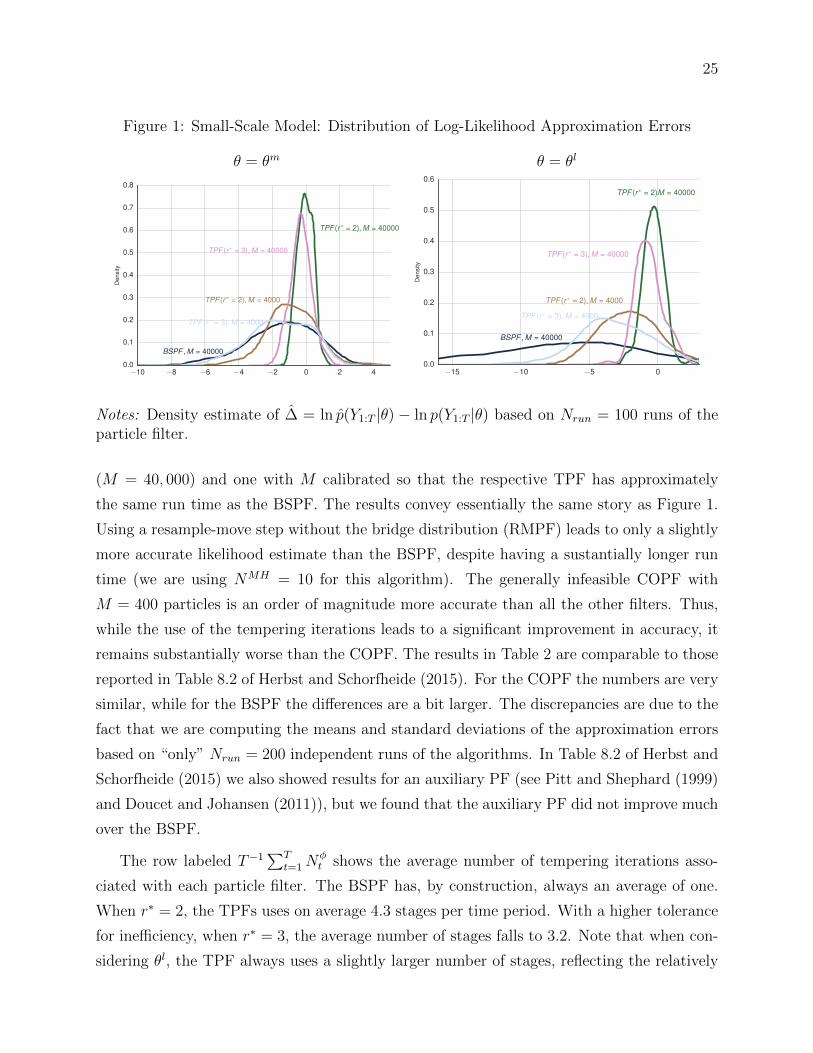
Figure 1 displays density estimates based on Nrun = 100 for the sampling distribution of
∆ associated with the BSPF and the four variants of the TPF for θ = θm (left panel) and
θ = θl (right panel). For θ = θm, the TPF (r∗ = 2) with M = 40, 000 (the green line) is
the most accurate of all the filters considered, with ∆ distributed tightly around zero. The
distribution of ∆ associated with TPF (r∗ = 3) with M = 40, 000 is slightly more disperse,
with a larger left tail, as the higher tolerance for particle inefficiency translates into a higher
variance for the likelihood estimate. Reducing the number of particles to M = 4, 000 for
both of these filters results in a higher variance estimate of the likelihood. The most poorly
performing TPF (with r∗ = 3 and M = 4, 000) is associated with a distribution for ∆ that
is similar to the one associated with the BSPF that uses M = 40, 000. Overall, the TPF
compares favorably with the BSPF when θ = θm. The performance differences become even
more stark when we consider θ = θl; depicted in the right panel of Figure 1. While the
sampling distributions indicate that the likelihood estimates are less accurate for all the
particles filters, the BSPF deteriorates by the largest amount. The TPF, by targeting an
inefficiency ratio, adaptively adjusts to account for the relatively worse fit of θl.
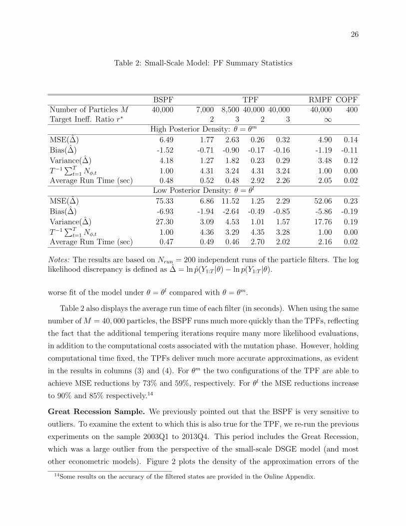
Table 2 displays summary statistics for the likelihood approximation errors as well as
information about the average number of stages and run time of each filter. We compute
the mean-squared error (MSE), the bias, and the variance of ∆ across Nrun = 200 runs. For
each r∗, we run two versions of the TPF: one with same number of particles as the BSPF
25
Figure 1: Small-Scale Model: Distribution of Log-Likelihood Approximation Errors
θ = θm θ = θl
−10 −8 −6 −4 −2 0 2 40.0
0.1
0.2
0.3
0.4
0.5
0.6
0.7
0.8
Den
sity
TPF (r ∗ = 2), M = 40000
TPF (r ∗ = 2), M = 4000
TPF (r ∗ = 3), M = 40000
TPF (r ∗ = 3), M = 4000
BSPF , M = 40000
−15 −10 −5 00.0
0.1
0.2
0.3
0.4
0.5
0.6
Den
sity
TPF (r ∗ = 2)M = 40000
TPF (r ∗ = 2), M = 4000
TPF (r ∗ = 3), M = 40000
TPF (r ∗ = 3), M = 4000
BSPF , M = 40000
Notes: Density estimate of ∆ = ln p(Y1:T |θ) − ln p(Y1:T |θ) based on Nrun = 100 runs of theparticle filter.
(M = 40, 000) and one with M calibrated so that the respective TPF has approximately
the same run time as the BSPF. The results convey essentially the same story as Figure 1.
Using a resample-move step without the bridge distribution (RMPF) leads to only a slightly
more accurate likelihood estimate than the BSPF, despite having a sustantially longer run
time (we are using NMH = 10 for this algorithm). The generally infeasible COPF with
M = 400 particles is an order of magnitude more accurate than all the other filters. Thus,
while the use of the tempering iterations leads to a significant improvement in accuracy, it
remains substantially worse than the COPF. The results in Table 2 are comparable to those
reported in Table 8.2 of Herbst and Schorfheide (2015). For the COPF the numbers are very
similar, while for the BSPF the differences are a bit larger. The discrepancies are due to the
fact that we are computing the means and standard deviations of the approximation errors
based on “only” Nrun = 200 independent runs of the algorithms. In Table 8.2 of Herbst and
Schorfheide (2015) we also showed results for an auxiliary PF (see Pitt and Shephard (1999)
and Doucet and Johansen (2011)), but we found that the auxiliary PF did not improve much
over the BSPF.
The row labeled T−1∑T
t=1Nφt shows the average number of tempering iterations asso-
ciated with each particle filter. The BSPF has, by construction, always an average of one.
When r∗ = 2, the TPFs uses on average 4.3 stages per time period. With a higher tolerance
for inefficiency, when r∗ = 3, the average number of stages falls to 3.2. Note that when con-
sidering θl, the TPF always uses a slightly larger number of stages, reflecting the relatively
26
Table 2: Small-Scale Model: PF Summary Statistics
BSPF TPF RMPF COPFNumber of Particles M 40,000 7,000 8,500 40,000 40,000 40,000 400Target Ineff. Ratio r∗ 2 3 2 3 ∞
High Posterior Density: θ = θm
MSE(∆) 6.49 1.77 2.63 0.26 0.32 4.90 0.14
Bias(∆) -1.52 -0.71 -0.90 -0.17 -0.16 -1.19 -0.11
Variance(∆) 4.18 1.27 1.82 0.23 0.29 3.48 0.12
T−1∑T
t=1 Nφ,t 1.00 4.31 3.24 4.31 3.24 1.00 0.00Average Run Time (sec) 0.48 0.52 0.48 2.92 2.26 2.05 0.02
Low Posterior Density: θ = θl
MSE(∆) 75.33 6.86 11.52 1.25 2.29 52.06 0.23
Bias(∆) -6.93 -1.94 -2.64 -0.49 -0.85 -5.86 -0.19
Variance(∆) 27.30 3.09 4.53 1.01 1.57 17.76 0.19
T−1∑T
t=1 Nφ,t 1.00 4.36 3.29 4.35 3.28 1.00 0.00Average Run Time (sec) 0.47 0.49 0.46 2.70 2.02 2.16 0.02
Notes: The results are based on Nrun = 200 independent runs of the particle filters. The loglikelihood discrepancy is defined as ∆ = ln p(Y1:T |θ)− ln p(Y1:T |θ).
worse fit of the model under θ = θl compared with θ = θm.
Table 2 also displays the average run time of each filter (in seconds). When using the same
number ofM = 40, 000 particles, the BSPF runs much more quickly than the TPFs, reflecting
the fact that the additional tempering iterations require many more likelihood evaluations,
in addition to the computational costs associated with the mutation phase. However, holding
computational time fixed, the TPFs deliver much more accurate approximations, as evident
in the results in columns (3) and (4). For θm the two configurations of the TPF are able to
achieve MSE reductions by 73% and 59%, respectively. For θl the MSE reductions increase
to 90% and 85% respectively.14
Great Recession Sample. We previously pointed out that the BSPF is very sensitive to
outliers. To examine the extent to which this is also true for the TPF, we re-run the previous
experiments on the sample 2003Q1 to 2013Q4. This period includes the Great Recession,
which was a large outlier from the perspective of the small-scale DSGE model (and most
other econometric models). Figure 2 plots the density of the approximation errors of the
14Some results on the accuracy of the filtered states are provided in the Online Appendix.

27
Figure 2: Small-Scale Model: Distribution of Log-Likelihood Approximation Errors, GreatRecession Sample
θ = θm θ = θl
−350 −300 −250 −200 −150 −100 −50 00.00
0.05
0.10
0.15
0.20
0.25
0.30
Den
sity
TPF (r ∗ = 2), M = 40000
TPF (r ∗ = 2), M = 4000
TPF (r ∗ = 3), M = 40000
TPF (r ∗ = 3), M = 4000
BSPF , M = 40000
−350 −300 −250 −200 −150 −100 −50 00.00
0.05
0.10
0.15
0.20
0.25
Den
sity
TPF (r ∗ = 2), M = 40000
TPF (r ∗ = 2), M = 4000
TPF (r ∗ = 3), M = 40000
TPF (r ∗ = 3), M = 4000BSPF , M = 40000
Notes: Density estimate of ∆ = ln p(Y1:T |θ) − ln p(Y1:T |θ) based on Nrun = 100 runs of theparticle filters.
log likelihood estimates associated with each of the filters. The difference in the distribution
of approximation errors between the BSPF and the TPFs is massive. For θ = θm and
θ = θl, the approximation errors associated with the BSPF are concentrated in the range of
−200 to −300, almost two orders of magnitude larger than the errors associated with the
TPFs. This happens because the large drop in output in 2008Q4 is not predicted by the
forward simulation in the BSPF. In turn, the filter collapses, in the sense that the likelihood
increment in that quarter is estimated using essentially only one particle.
Table 3 tabulates the results for each of the filters. Consistent with Figure 2, the MSEs
associated with the log-likelihood estimate of the BSPF are 47, 534 and 79, 473 for θ = θm and
θ = θl, respectively, compared to 85 and 150 for the better of the two TPF configurations,
holding computational time fixed. If we increase the number of particles to M = 40, 000,
then for θ = θm the TPF (r∗ = 2) with has an MSE of 33, which is about 1,425 times smaller
than the BSPF and only raises the computational time by a factor of 10. A key driver of
this result is the adaptive nature of the TPF. While the average number of stages used is
about 5 for r∗ = 2 and 4 for r∗ = 3, for t = 2008Q4 – the period with the largest outlier –
the TPF uses about 15 stages, on average.
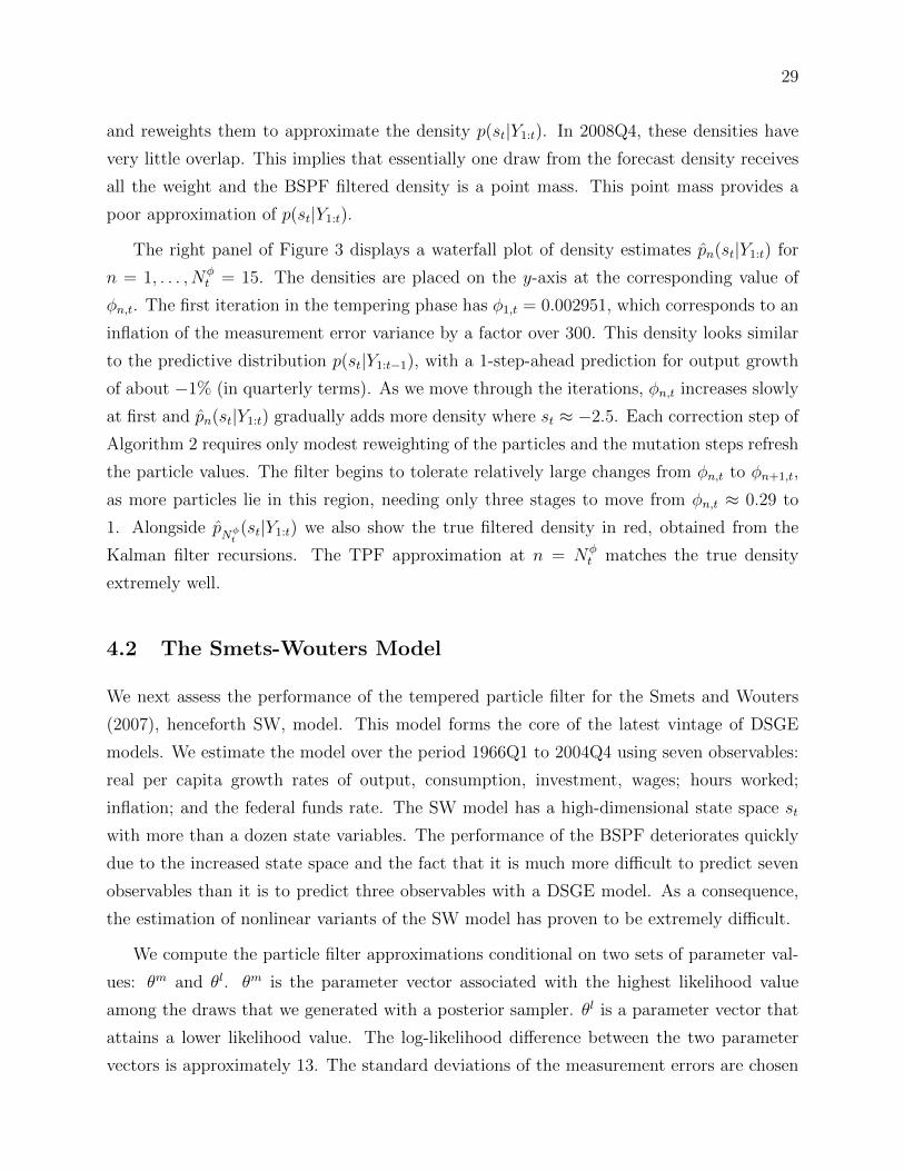
Figure 3 provides an illustration of why the TPF provides much more accurate approxima-
tions than the BSPF. We focus on one particular state, namely model-implied output growth,
which is observed output growth minus its measurement error. We focus on t = 2008Q4. The

28
Table 3: Small-Scale Model: PF Summary Statistics – The Great Recession
BSPF TPFNumber of Particles M 40,000 5,500 7,000 40,000 40,000Target Ineff. Ratio r∗ 2 3 2 3
High Posterior Density: θ = θm
MSE(∆) 47,533.80 85.02 143.88 33.37 66.99
Bias(∆) -215.22 -8.54 -11.49 -5.33 -7.74
Variance(∆) 1,215.88 12.08 11.78 4.94 7.08
T−1∑T
t=1Nφ,t 1.00 5.13 3.88 5.10 3.86Average Run Time (sec) 0.26 0.27 0.27 2.02 1.42
Low Posterior Density: θ = θl
MSE(∆) 79,473.19 150.63 244.44 64.03 116.84
Bias(∆) -278.88 -11.72 -15.14 -7.62 -10.47
Variance(∆) 1,700.42 13.25 15.14 5.92 7.20
T−1∑T
t=1Nφ,t 1.00 5.36 4.06 5.32 4.04Average Run Time (sec) 0.27 0.29 0.28 2.12 1.49
Notes: The results are based on Nrun = 200 independent runs of the particle filters. The loglikelihood discrepancy is defined as ∆ = ln p(Y1:T |θ)− ln p(Y1:T |θ).
Figure 3: Small-Scale Model: BSPF versus TPF in 2008Q4
BSPF TPF
4 3 2 1 0 1 20.0
0.5
1.0
1.5
2.0
2.5
3.0
3.5Forecast DensityBSPF Filtered DensityTrue Filtered Density
−4 −3 −2 −1 0 1 2φn
0.00.2
0.40.6
0.81.0
0.0
0.5
1.0
1.5
2.0
2.5
3.0
3.5
Notes: Here t = 2008Q4 and st equals model-implied output growth. Left panel: forecastdensity p(st|Y1:t−1), BSPF filtered density p(st|Y1:t), and true filtered density p(st|Yt−1).Right panel: forecast density p(st|Y1:t−1) (blue), waterfall plot of density estimates pn(st|Y1:t)for n = 1, . . . , Nφ
t , and true filtered density p(st|Y1:t) (red).
left panel depicts the BSPF approximations p(st|Y1:t−1) and p(st|Y1:t) as well as the “true”
density p(st|Y1:t). The BSPF essentially generates draws from the forecast density p(st|Y1:t−1)
29
and reweights them to approximate the density p(st|Y1:t). In 2008Q4, these densities have
very little overlap. This implies that essentially one draw from the forecast density receives
all the weight and the BSPF filtered density is a point mass. This point mass provides a
poor approximation of p(st|Y1:t).
The right panel of Figure 3 displays a waterfall plot of density estimates pn(st|Y1:t) for
n = 1, . . . , Nφt = 15. The densities are placed on the y-axis at the corresponding value of
φn,t. The first iteration in the tempering phase has φ1,t = 0.002951, which corresponds to an
inflation of the measurement error variance by a factor over 300. This density looks similar
to the predictive distribution p(st|Y1:t−1), with a 1-step-ahead prediction for output growth
of about −1% (in quarterly terms). As we move through the iterations, φn,t increases slowly
at first and pn(st|Y1:t) gradually adds more density where st ≈ −2.5. Each correction step of
Algorithm 2 requires only modest reweighting of the particles and the mutation steps refresh
the particle values. The filter begins to tolerate relatively large changes from φn,t to φn+1,t,
as more particles lie in this region, needing only three stages to move from φn,t ≈ 0.29 to
1. Alongside pNφt(st|Y1:t) we also show the true filtered density in red, obtained from the
Kalman filter recursions. The TPF approximation at n = Nφt matches the true density
extremely well.
4.2 The Smets-Wouters Model
We next assess the performance of the tempered particle filter for the Smets and Wouters
(2007), henceforth SW, model. This model forms the core of the latest vintage of DSGE
models. We estimate the model over the period 1966Q1 to 2004Q4 using seven observables:
real per capita growth rates of output, consumption, investment, wages; hours worked;
inflation; and the federal funds rate. The SW model has a high-dimensional state space st
with more than a dozen state variables. The performance of the BSPF deteriorates quickly
due to the increased state space and the fact that it is much more difficult to predict seven
observables than it is to predict three observables with a DSGE model. As a consequence,
the estimation of nonlinear variants of the SW model has proven to be extremely difficult.
We compute the particle filter approximations conditional on two sets of parameter val-
ues: θm and θl. θm is the parameter vector associated with the highest likelihood value
among the draws that we generated with a posterior sampler. θl is a parameter vector that
attains a lower likelihood value. The log-likelihood difference between the two parameter
vectors is approximately 13. The standard deviations of the measurement errors are chosen

30
Figure 4: Smets-Wouters Model: Distribution of Log-Likelihood Approximation Errors
θ = θm θ = θl
−700 −600 −500 −400 −300 −200 −100 0 1000.000
0.002
0.004
0.006
0.008
0.010
0.012
0.014
0.016
0.018
Den
sity
TPF (r ∗ = 2), M = 40000
TPF (r ∗ = 2), M = 4000
TPF (r ∗ = 3), M = 40000
TPF (r ∗ = 3), M = 4000
BSPF , M = 40000
−600 −500 −400 −300 −200 −100 0 100 2000.000
0.002
0.004
0.006
0.008
0.010
0.012
0.014
0.016
Den
sity
TPF (r ∗ = 2), M = 40000
TPF (r ∗ = 2), M = 4000
TPF (r ∗ = 3), M = 40000
TPF (r ∗ = 3), M = 4000
BSPF , M = 40000
Notes: Density estimate of ∆ = ln p(Y1:T |θm) − ln p(Y1:T |θm) based on Nrun = 100 runs ofthe particle filters and NMH = 10.
to be approximately 20% of the sample standard deviation of the time series.15 For compar-
ison purposes, the parameter values and the data are identical to the ones used in Chapter
8 of Herbst and Schorfheide (2015) and their values are tabulated in the Online Appendix.
For the small-scale New Keynesian model we only used one mutation step at each tem-
pering stage, i.e., NMH = 1, which worked well. After some experimentation with the SW
model, we increased the number of mutation steps to NMH = 10. This allows the particles
to better adapt to the current density because it increases the probability that their values
change. The subsequently-reported results are based on NMH = 10, whereas results for
NMH = 1 are relegated to the Online Appendix.
Figure 4 displays density estimates of the approximation errors associated with the log-
likelihood estimates under θ = θm and θ = θl. We use M = 40, 000 particles for the BSPF.
For the TPF, we use M = 4, 000 or M = 40, 000, consider r∗ = 2 and r∗ = 3 and set c∗ = 0.3
in the mutation step. Under both parameter values, the BSPF exhibits the most bias, with
its likelihood estimates substantially below the true likelihood value. The distribution of the
bias falls mainly between −400 and −100. Thus, drawing from the posterior distribution
of the SW model using a particle MCMC algorithm based on the BSPF, would be nearly
impossible. The TPFs perform better, although they also underestimate the likelihood by a
15The standard deviations for the measurement errors are 0.1731 (output growth), 0.1394 (consumptiongrowth), 0.4515 (investment growth), 0.1128 (wage growth), 0.5838 (log hours), 0.1230 (inflation), and 0.1653(interest rates).

31
Table 4: SW Model: PF Summary Statistics
BSPF TPFNumber of Particles M 40,000 2,000 2,800 40,000 40,000Target Ineff. Ratio r∗ 2 3 2 3
High Posterior Density: θ = θm
MSE(∆) 63,881.68 1,164.15 1,135.35 57.79 93.05
Bias(∆) -245.64 -30.94 -30.41 -6.55 -8.51
Variance(∆) 3,543.79 206.58 210.51 14.92 20.56
T−1∑T
t=1Nφ,t 1.00 6.12 4.69 6.07 4.68Average Run Time (sec) 3.33 3.00 3.49 62.57 48.85
Low Posterior Density: θ = θl
MSE(∆) 69,612.88 1,489.59 1,993.62 108.39 191.56
Bias(∆) -255.06 -36.20 -41.66 -9.36 -12.36
Variance(∆) 4,559.09 179.24 258.30 20.82 38.88
T−1∑T
t=1Nφ,t 1.00 6.18 4.76 6.14 4.71Average Run Time (sec) 3.28 3.34 3.33 63.98 49.56
Notes: Results are based on Nrun = 200 independent runs of the particle filters and NMH =10. The log likelihood discrepancy is defined as ∆ = ln p(Y1:T |θ)− ln p(Y1:T |θ).
large amount.
Table 4 underscores the results in Figure 4. The best-performing TPF reduces the MSE
in the log-likelihood approximation for θm from 63,881.68 to 58 for θm. This increased
performance comes at a computational cost: the TPF (r∗ = 2),M = 40, 000 filter takes
about 62 seconds, while the BSPF takes only about 3 seconds. However, even if we reduce
the number of particles for the TPFs to achieve approximately the same run time as the
BSPF (see columns 3 and 4), the TPFs come out ahead by a wide margin. Across the two
parameter values and the two filter specifications, the TPF still is able to reduce the MSE
by a factor of at least 35. We conclude that holding computational time fixed, tempering
leads to a significant improvement in the accuracy of the likelihood approximation.
5 Conclusion
We developed a particle filter that automatically adapts the proposal distribution for the
particles sjt to the current observation yt. We start with a forward simulation of the state-
transition equation under an inflated measurement error variance and then gradually reduce

32
the variance to its nominal level. In each step, the particle values and weights change so
that the distribution slowly adapts to p(sjt |yt, sjt−1). We demonstrate in two DSGE model
applications that controlling for run time the algorithm generates significantly more accurate
approximations than the standard bootstrap particle filter, in particular in instances in
which the model generates very inaccurate one-step-ahead predictions of yt. The tempering
iterations can also be used to improve a particle filter with a more general initial proposal
distribution than the BSPF. Moreover, our filter can be easily embedded in particle MCMC
algorithms.
References
Andreasen, M. M. (2013): “Non-Linear DSGE Models and the Central Difference Kalman
Filter,” Journal of Applied Econometrics, 28(6), 929–955.
Andrieu, C., A. Doucet, and R. Holenstein (2010): “Particle Markov Chain Monte
Carlo Methods,” Journal of the Royal Statistical Society Series B, 72(3), 269–342.
Arulampalam, S., S. Maskell, N. Gordon, and T. Clapp (2002): “A Tutorial on
Particle Filters for Online Nonlinear/Non-Gaussian Bayesian Tracking,” IEEE Transac-
tions on Signal Processing, 50(2), 174–188.
Beskos, A., A. Jasra, N. Kantas, and A. H. Thiery (2014): “On the Convergence of
Adaptive Sequential Monte Carlo Methods,” arXiv Working Paper.
Bognanni, M., and E. P. Herbst (2015): “Estimating (Markov-Switching) VAR Models
without Gibbs Sampling: A Sequential Monte Carlo Approach,” Finance and Economics
Discussion Paper Series, Board of Governors, 2015-116(116), 154.
Cappe, O., S. J. Godsill, and E. Moulines (2007): “An Overview of Existing Methods
and Recent Advances in Sequential Monte Carlo,” Proceedings of the IEEE, 95(5), 899–
924.
Cappe, O., E. Moulines, and T. Ryden (2005): Inference in Hidden Markov Models.
Springer Verlag, New York.
Chopin, N. (2002): “A Sequential Particle Filter for Static Models,” Biometrika, 89(3),
539–551.
(2004): “Central Limit Theorem for Sequential Monte Carlo Methods and Its
Application to Bayesian Inference,” Annals of Statistics, 32(6), 2385–2411.

33
Creal, D. (2007): “Sequential Monte Carlo Samplers for Bayesian DSGE Models,”
Manuscript, University Chicago Booth.
(2012): “A Survey of Sequential Monte Carlo Methods for Economics and Finance,”
Econometric Reviews, 31(3), 245–296.
Del Moral, P. (2004): Feynman-Kac Formulae. Springer Verlag.
(2013): Mean Field Simulation for Monte Carlo Integration. Chapman & Hall/CRC,
Boca Raton.
Del Moral, P., A. Doucet, and A. Jasra (2006): “Sequential Monte Carlo Samplers,”
Journal of the Royal Statistical Society, Series B, 68(Part 3), 411–436.
(2012): “An AdaptiveSequential Monte Carlo Method for Approximate Bayesian
Computation,” Statistical Computing, 22, 1009–1020.
Doucet, A., and A. M. Johansen (2011): “A Tutorial on Particle Filtering and Smooth-
ing: Fifteen Years Later,” in Handook of Nonlinear Filtering, ed. by D. Crisan, and B. Ro-
zovsky. Oxford University Press, Oxford.
Durham, G., and J. Geweke (2014): “Adaptive Sequential Posterior Simulators for
Massively Parallel Computing Environments,” in Advances in Econometrics, ed. by I. Jeli-
azkov, and D. Poirier, vol. 34, chap. 6, pp. 1–44. Emerald Group Publishing Limited, West
Yorkshire.
Fernandez-Villaverde, J., and J. F. Rubio-Ramırez (2007): “Estimating Macroeco-
nomic Models: A Likelihood Approach,” Review of Economic Studies, 74(4), 1059–1087.
Geweke, J., and B. Frischknecht (2014): “Exact Optimization By Means of Sequen-
tially Adaptive Bayesian Learning,” Mimeo.
Godsill, S. J., and T. Clapp (2001): “Improvement Strategies for Monte Carlo Particle
Filters,” in Sequential Monte Carlo Methods in Practice, ed. by A. Doucet, N. De Freitas,
and N. Gordon, pp. 139–158. Springer Verlag, New York.
Gordon, N., D. Salmond, and A. F. Smith (1993): “Novel Approach to Nonlinear/Non-
Gaussian Bayesian State Estimation,” Radar and Signal Processing, IEE Proceedings F,
140(2), 107–113.
Gust, C., E. Herbst, D. Lopez-Salido, and M. E. Smith (2017): “The Empirical
Implications of the Interest-Rate Lower Bound,” American Economic Review, forthcoming.

34
Herbst, E., and F. Schorfheide (2014): “Sequential Monte Carlo Sampling for DSGE
Models,” Journal of Applied Econometrics, 29(7), 1073–1098.
(2015): Bayesian Estimation of DSGE Models. Princeton University Press, Prince-
ton.
Jasra, A., D. A. Stephens, A. Doucet, and T. Tsagaris (2011): “Inference for Levy-
Driven Stochastic Volatility Models via Adaptive Sequential Monte Carlo,” Scandinavian
Journal of Statistics, 38, 1–22.
Johansen, A. M. (2016): “On Blocks, Tempering and Particle MCMC for Systems Iden-
tification,” Manuscript, University of Warwick.
Kollmann, R. (2015): “Tractable Latent State Filtering for Non-Linear DSGE Models
Using a Second-Order Approximation and Pruning,” Computational Economics, 45(2),
239–260.
Liu, J. S. (2001): Monte Carlo Strategies in Scientific Computing. Springer Verlag, New
York.
Neal, R. M. (1998): “Annealed Importance Sampling,” Technical Report, Department of
Statistics, University of Toronto, 9805.
Pitt, M. K., and N. Shephard (1999): “Filtering via Simulation: Auxiliary Particle
Filters,” Journal of the American Statistical Association, 94(446), 590–599.
Pitt, M. K., R. d. S. Silva, P. Giordani, and R. Kohn (2012): “On Some Properties
of Markov Chain Monte Carlo Simulation Methods Based on the Particle Filter,” Journal
of Econometrics, 171(2), 134–151.
Schafer, C., and N. Chopin (2013): “Sequential Monte Carlo on Large Binary Sampling
Spaces,” Statistical Computing, 23, 163–184.
Smets, F., and R. Wouters (2007): “Shocks and Frictions in U.S. Business Cycles: A
Bayesian DSGE Approach,” American Economic Review, 97(3), 586–608.
White, H. (2001): Asymptotic Theory For Econometricians. Academic Press, New York.
Zhou, Y., A. M. Johansen, and J. A. Aston (2015): “Towards Automatic Model
Comparison: An Adaptive Sequential Monte Carlo Approach,” arXiv Working Paper,
1303.3123v2.

Online Appendix A-1
Online Appendix for
Tempered Particle Filtering
Edward Herbst and Frank Schorfheide
A Theoretical Derivations
A.1 Monotonicity of Inefficiency Ratio
Recall the definitions
ej,t =1
2(yt −Ψ(sj,n−1
t ))′Σ−1u (yt −Ψ(sj,n−1
t ))
and
wj,nt (φn) =
(φnφn−1
)ny/2exp[−(φn − φn−1)ej,t].
Provided that the particles had been resampled and W j,n−1t = 1, the inefficiency ratio can
be manipulated as follows:
InEff(φn) =1M
∑Mj=1
(wj,nt (φn)
)2(1M
∑Mj=1 w
j,nt (φn)
)2
=
1M
∑Mj=1
(φnφn−1
)nyexp[−2(φn − φn−1)ej,t](
1M
∑Mj=1
(φnφn−1
)ny/2exp[−(φn − φn−1)ej,t]
)2
=1M
∑Mj=1 exp[−2(φn − φn−1)ej,t](
1M
∑Mj=1 exp[−(φn − φn−1)ej,t]
)2
=A1(φn)
A2(φn).
Note that for φn = φn−1, we obtain ESS(φn) = 1. We now will show that the inefficiency
ratio is monotonically increasing on the interval φn ∈ [φn−1, 1]. Differentiating with respect

Online Appendix A-2
to φn yields (we use the superscript (1) to denote first derivatives):
InEff(1)(φn) =A
(1)1 (φn)A2(φn)− A1(φn)A
(1)2 (φn)
[A2(φn)]2,
where
A(1)1 (φn) = − 2
M
M∑j=1
ej,t exp[−2(φn − φn−1)ej,t]
A(1)2 (φn) =
(2
M
M∑j=1
exp[−(φn − φn−1)ej,t]
)(− 1
M
M∑j=1
ej,t exp[−(φn − φn−1)ej,t]
).
The denominator in InEff(1)(φn) is always non-negative and strictly different from zero. Thus,
we can focus on the numerator:
A(1)1 (φn)A2(φn)− A1(φn)A
(1)2 (φn)
=
(− 2
M
M∑j=1
ej,t exp[−2(φn − φn−1)ej,t]
)(1
M
M∑j=1
exp[−(φn − φn−1)ej,t]
)2
−(
1
M
M∑j=1
exp[−2(φn − φn−1)ej,t]
)(2
M
M∑j=1
exp[−(φn − φn−1)ej,t]
)
×(− 1
M
M∑j=1
ej,t exp[−(φn − φn−1)ej,t]
)
= 2
(1
M
M∑j=1
exp[−(φn − φn−1)ej,t]
)
×[(
1
M
M∑j=1
exp[−2(φn − φn−1)ej,t]
)(1
M
M∑j=1
ej,t exp[−(φn − φn−1)ej,t]
)
−(
1
M
M∑j=1
ej,t exp[−2(φn − φn−1)ej,t]
)(1
M
M∑j=1
exp[−(φn − φn−1)ej,t]
)].
To simplify the notation, we now write ej instead of ej,t, let λ = φn − φn−1 ≥ 0, and
define
xj = exp[−(φn − φn−1)ej] =1
exp[λej].

Online Appendix A-3
Note that 0 < xj ≤ 1 and ej ≥ 0. We scale the numerator of InEff(1)(φn) by M3/2, which
leads to
M3
2
[A(1)(φn)A2(φn)− A1(φn)A
(1)2 (φn)
]=
(M∑j=1
xj
)[(M∑j=1
x2j
)(M∑j=1
ejxj
)−(
M∑j=1
ejx2j
)(M∑j=1
xj
)].
Thus, the sign of InEff(1)(φn) is determined by the sign of
∆M =
(M∑j=1
ejxj
)(M∑j=1
x2j
)−(
M∑j=1
ejx2j
)(M∑j=1
xj
).
Consider the special case of M = 2:
∆M = +e1x1x21 + e1x1x
22 + e2x2x
21 + e2x2x
22
−e1x21x1 − e1x
21x2 − e2x
22x1 − e2x
22x2
= e1x1x2(x2 − x1) + e2x1x2(x1 − x2)
= x1x2(x2 − x1)(e1 − e2)
= x1x2
(1
exp[λe2]− 1
exp[λe1]
)(e1 − e2)
≥ 0,
because for any λ ≥ 0
sign
(1
exp[λe2]− 1
exp[λe1]
)= sign(e1 − e2).

Online Appendix A-4
Now consider the general case:
∆M =M∑j=1
M∑l=1
ejxjx2l −
M∑j=1
M∑l=1
ejx2jxl
=M∑j=1
∑l 6=j
ejxjx2l −
M∑j=1
∑l 6=j
ejx2jxl
=M∑j=1
∑l 6=j
ejxjxl(xl − xj)
=M∑j=1
∑l<j
ejxjxl(xl − xj) +M∑l=1
∑j<l
ejxjxl(xl − xj)
=M∑j=1
∑l<j
ejxjxl(xl − xj) +M∑j=1
∑l<j
elxlxj(xj − xl)
=M∑j=1
∑l<j
ejxjxl(xl − xj)(ej − el)
The manipulations are similar to the case of M = 2. The first equality is obtained from the
definition of ∆M . The second equality is obtained by noticing that the j = l terms cancel.
In the third equality we combine the terms that arise in the two double summations. Now
imagine that the right-hand-side terms are arranged in a matrix where j is the row index
and l the column index:0 e1x1x2(x2 − x1) e1x1x3(x3 − x1)
e2x2x1(x1 − x2) 0 e2x2x3(x3 − x2)
e3x3x1(x1 − x3) e3x3x2(x2 − x3) 0
The fourth equality is obtained by separately summing the terms below and above the di-
agonal. The fifth equality is obtained by switching the j and the l index in the second
summation. Finally, the last equality is obtained by combining the two double sums. Be-
cause,
sign
(1
exp[λel]− 1
exp[λej]
)= sign(ej − el),

Online Appendix A-5
we can deduce that
∆M ≥ 0
and conclude that the inefficiency ratio InEff(φn) is increasing in φn. �
A.2 Proofs for Section 3.1
The proofs in this section closely follow Chopin (2004) and Herbst and Schorfheide (2014).
Throughout this section, we will assume that h(·) is scalar and we use absolute values |h|instead of a general norm ‖h‖. Extensions to vector-valued-h functions are straightforward.
We use C to denote a generic constant. We will make repeated use of the following moment
bound for r > 1
E[∣∣X − E[X]
∣∣r] ≤ Cr(E[∣∣X∣∣r]+
∣∣E[X]∣∣r) (A.1)
≤ 2CrE[∣∣X∣∣r],
where Cr = 1 for r = 1 and Cr = 2r−1 for r > 1. The first inequality follows from the Cr
inequality and the second inequality follows from Jensen’s inequality.
We will make use of the following SLLN (Markov, see White (2001) p. 33): Let {Zj} be
a sequence of independent random variables with finite means µj = E[Zj]. If for some δ > 0,∑∞j=1 E
[|Zj − µj|1+δ
]/j1+δ < ∞, then 1
M
∑Mj=1 Zj − µj
a.s−→ 0. Note that E[|Zj − µj|1+δ
]<
C <∞ implies that the summability condition is satisfied because∑∞
j=1(1/j)1+δ <∞.
Recall that under a multivariate Gaussian measurement error distribution, the density
pn(yt|st) can be bounded from above. Thus, pn(yt|st) ∈ Hnt
and ωj,nt ∈ Hnt
for any t and n.
Moreover, for any h(st, st−1) ∈ Hnt , we can deduce that h(·) = h(·)ωj,nt ∈ Hn
t .
Proof of Lemma 1.
Part (i). The forward iteration of the state-transition equation amounts to drawing sjt
from the density p(st|sj,Nφ
t−1 ). Use Ep(st|sj,N
φ
t−1 )[·] to denote expectations under this density and

Online Appendix A-6
consider the decomposition:
h1t|t−1 −
∫ ∫h(st, st−1)p(st, st−1|Y1:t−1)dstdst−1 (A.2)
=1
M
M∑j=1
(h(sj,1t , s
Nφ
t−1)− Ep(st|sj,N
φ
t−1 )[h(st, s
j,Nφ
t−1 )]
)W j,Nφ
t−1
+1
M
M∑j=1
(Ep(st|sj,N
φ
t−1 )[h(st, s
j,Nφ
t−1 )]W j,Nφ
t−1 −∫ ∫
h(st, st−1)p(st, st−1|Y1:t−1)dstdst−1
)= I + II.
We now show that terms I and II in (A.2) converge to zero. According to the above
definition
I =1
M
M∑j=1
(h(sjt , s
j,Nφ
t−1 )− Ep(·|sj,N
φ
t−1 )[h]
)W j,Nφ
t−1 .
Here we used the abbreviation
Ep(·|st−1)[h] = Ep(st|st−1)[h(st, st−1)].
Conditional on the particles {sj,Nφ
t−1 ,Wj,Nφ
t−1 } the summands in term I form a triangular array
of mean-zero random variables that within each row are independently distributed. In Al-
gorithm 4 the particles were resampled during the t − 1 tempering iteration Nφ, such that
WNφ
t−1 = 1. Using the bound
Ep(st|st−1)
[∣∣h(st, st−1)− Ep(·|st−1)[h]∣∣1+δ
]< C <∞
implied by the definition of H1t , we can apply the SLLN to deduce that term I
a.s.−→ 0.
The second term in (A.2) takes the form
II =1
M
M∑j=1
(Ep(·|sjt−1)[h]−
∫ ∫h(st, st−1)p(st, st−1|Y1:t−1)dstdst−1
).
The definition of H1t implies that Ep(·|st−1)[h] ∈ HNφ
t−1. The almost-sure convergence to zero of
term II can now be deduced from the recursive Assumption 1. By combining the convergence

Online Appendix A-7
results for terms I and II we have established (34).
Part (ii). The convergences in (35) and (37) follow immediately from the fact that p1(yt|st) ∈H1t . Moreover, if h(st, st−1) ∈ H1
t , then h(st, st−1)p1(yt|st) ∈ H1t . Finally, p1(yt|st) > 0, which
implies that the almost-sure limit of the denominator in (35) is strictly positive.
Part (iii). To verify (36), let Ft,1,M denote the σ-algebra generated by the particles {sj,1t , sj,Nφ
t−1 ,Wj,1t }.
Moreover, define
E[h|Ft,1,M ] =1
M
M∑j=1
h(sj,1t , sj,Nφ
t−1 )W j,1t ,
and write
h1t −
∫h(st, st−1)p1(st, st−1|Y1:t)dst (A.3)
=1
M
M∑j=1
(h(sj,1t , s
j,Nφ
t−1 )− E[h|Ft,1,M ])
+
(1
M
M∑j=1
h(sj,1t , sNφ
t−1)W j,1t −
∫ ∫h(st, st−1)p1(st, st−1|Y1:t)dstdst−1
)
=1
M
M∑j=1
(h(sj,1t , s
j,Nφ
t−1 )− E[h|Ft,1,M ])
+
(h1t −
∫ ∫h(st, st−1)p1(st, st−1|Y1:t)dstdst−1
)= I + II.
From (35), we can immediately deduce that term II converges to zero almost surely. Re-
call that we are resampling the pairs (sj,nt , sj,Nφ
t−1 ). Thus, under multinomial resampling the
h(sj,1t , sj,Nφ
t )’s form a triangular array of i.i.d. random variables conditional on Ft,1,M . Using
Kolmogorov’s SLLN for i.i.d. sequences, it suffices to verify for that
E[∣∣h(sj,1t , s
j,Nφ
t )∣∣ ∣∣∣∣ Ft,1,M] <∞.
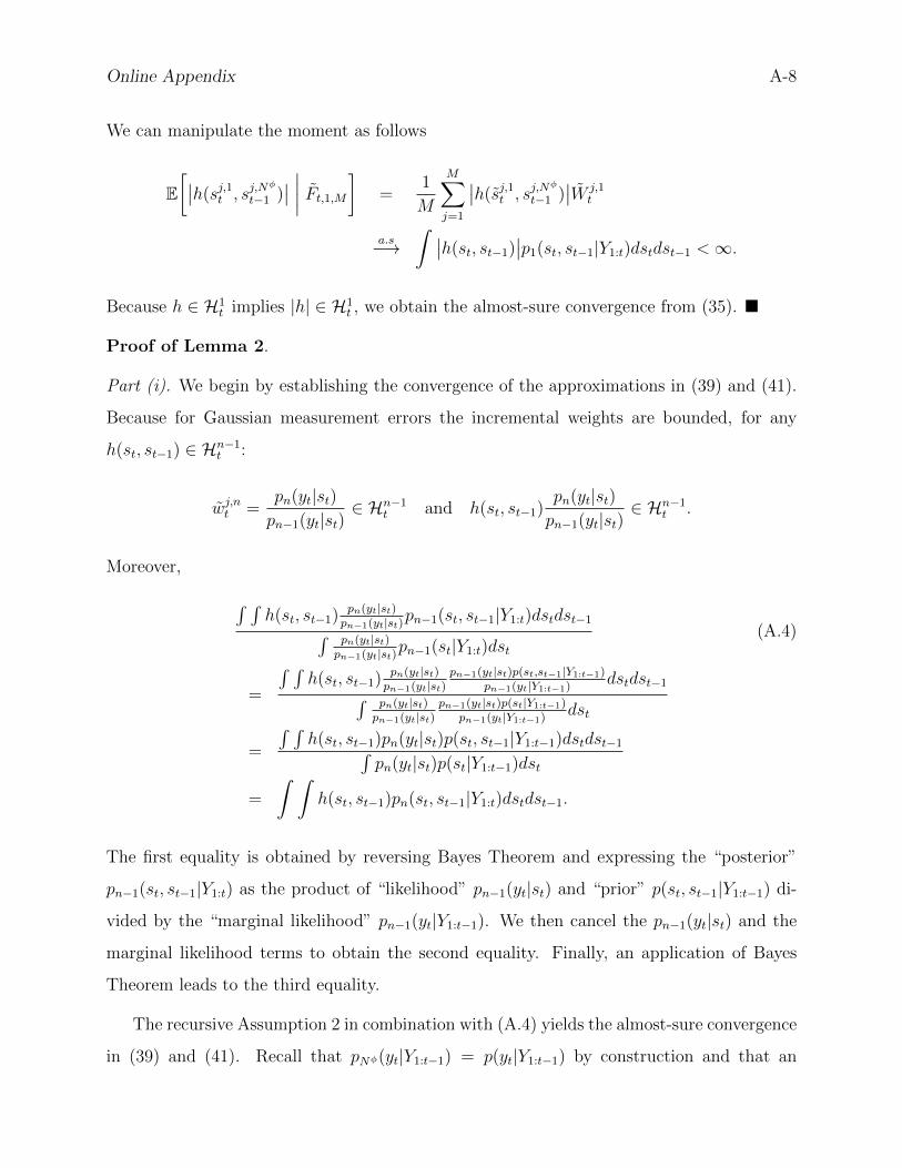
Online Appendix A-8
We can manipulate the moment as follows
E[∣∣h(sj,1t , s
j,Nφ
t−1 )∣∣ ∣∣∣∣ Ft,1,M] =
1
M
M∑j=1
∣∣h(sj,1t , sj,Nφ
t−1 )∣∣W j,1
t
a.s−→∫ ∣∣h(st, st−1)
∣∣p1(st, st−1|Y1:t)dstdst−1 <∞.
Because h ∈ H1t implies |h| ∈ H1
t , we obtain the almost-sure convergence from (35). �
Proof of Lemma 2.
Part (i). We begin by establishing the convergence of the approximations in (39) and (41).
Because for Gaussian measurement errors the incremental weights are bounded, for any
h(st, st−1) ∈ Hn−1t :
wj,nt =pn(yt|st)pn−1(yt|st)
∈ Hn−1t and h(st, st−1)
pn(yt|st)pn−1(yt|st)
∈ Hn−1t .
Moreover,
∫ ∫h(st, st−1) pn(yt|st)
pn−1(yt|st)pn−1(st, st−1|Y1:t)dstdst−1∫ pn(yt|st)pn−1(yt|st)pn−1(st|Y1:t)dst
(A.4)
=
∫ ∫h(st, st−1) pn(yt|st)
pn−1(yt|st)pn−1(yt|st)p(st,st−1|Y1:t−1)
pn−1(yt|Y1:t−1)dstdst−1∫ pn(yt|st)
pn−1(yt|st)pn−1(yt|st)p(st|Y1:t−1)
pn−1(yt|Y1:t−1)dst
=
∫ ∫h(st, st−1)pn(yt|st)p(st, st−1|Y1:t−1)dstdst−1∫
pn(yt|st)p(st|Y1:t−1)dst
=
∫ ∫h(st, st−1)pn(st, st−1|Y1:t)dstdst−1.
The first equality is obtained by reversing Bayes Theorem and expressing the “posterior”
pn−1(st, st−1|Y1:t) as the product of “likelihood” pn−1(yt|st) and “prior” p(st, st−1|Y1:t−1) di-
vided by the “marginal likelihood” pn−1(yt|Y1:t−1). We then cancel the pn−1(yt|st) and the
marginal likelihood terms to obtain the second equality. Finally, an application of Bayes
Theorem leads to the third equality.
The recursive Assumption 2 in combination with (A.4) yields the almost-sure convergence
in (39) and (41). Recall that pNφ(yt|Y1:t−1) = p(yt|Y1:t−1) by construction and that an

Online Appendix A-9
approximation of p1(yt|Y1:t−1) is generated in Step 2(a)iii of Algorithm 1. Together, this
leads to the approximation of the likelihood increment p(yt|Y1:t−1) in (23).
Part (ii). Resampling preserves the SLLN obtained for the correction step. Formally, the
convergence in (40) can be established with an argument similar to the one used in Step (iii)
of the proof of Lemma 1.
Part (iii). We begin with an outline of how to prove the convergence in (42) and will
subsequently provide some initially-omitted details. Abbreviate
EKn(·|st;st−1)[h] = EKn(st|st;st−1)[h(st, st−1)] =
∫h(st, st−1)Kn(st|st; st−1)dst,
which is a function of (st, st−1). We can decompose the Monte Carlo approximation from
the mutation step as follows:
1
M
M∑j=1
h(sj,nt , sj,Nφ
t−1 )W j,nt −
∫ ∫h(st, st−1)pn(st, st−1|Y1:t)dstdst−1 (A.5)
=1
M
M∑j=1
(h(sj,nt , sj,N
φ
t−1 )− EKn(·|sj,nt ;sj,N
φ
t−1 )[h]
)W j,nt
+1
M
M∑j=1
(EKn(·|sj,nt ;sj,N
φ
t−1 )[h]−
∫ ∫h(st, st−1)pn(st, st−1|Y1:t)dstdst−1
)W j,nt
= I + II, say.
By construction, conditional on the particles {sj,nt , sj,Nφ
t−1 ,Wj,nt }, term I is an average of
independent mean-zero random variables, which converges to zero.
The analysis of term II is more involved for two reasons. First, as previously highlighted,
EKn(·|sj,nt ;sj,N
φ
t−1 )[h] is a function not only of st but also of st−1. Second, while the invariance

Online Appendix A-10
property (21) implies that
∫EKn(·|st;st−1)[h]pn(st|yt, st−1)dst (A.6)
=
∫ (∫h(st, st−1)Kn(st|st; st−1)dst
)pn(st|yt, st−1)dst
=
∫h(st, st−1)
(∫Kn(st|st; st−1)pn(st|yt, st−1)dst
)dst
=
∫h(st, st−1)pn(st|yt, st−1)dst,
the summation over (sj,nt , sj,Nφ
t−1 ,Wj,nt ) generates an integral with respect to pn(st, st−1|Y1:t)
instead of pn(st|yt, st−1); see (40).
To obtain the expected value of EKn(·|st;st−1)[h] under the distribution pn(st, st−1|Y1:t),
notice that
pn(st, st−1|Y1:t) = pn(st, st−1|yt, Y1:t−1) (A.7)
= pn(st|st−1, yt, Y1:t−1)p(st−1|yt, Y1:t−1)
= pn(st|st−1, yt)p(st−1|yt, Y1:t−1).
The last equality holds because, using the first-order Markov structure of the state-space
model, we can write
pn(st|yt, st−1, Y1:t−1) =pn(yt|st, st−1, Y1:t−1)p(st|st−1, Y1:t−1)∫pn(yt|st, st−1, Y1:t−1)p(st|st−1, Y1:t−1)dst
=pn(yt|st)p(st|st−1)∫pn(yt|st)p(st|st−1)dst
= pn(st|yt, st−1).

Online Appendix A-11
Therefore, we obtain
∫ ∫EKn(·|st;st−1)[h]pn(st, st−1|Y1:t)dstdst−1 (A.8)
=
∫ (∫EKn(·|st;st−1)[h]pn(st|yt, st−1)dst
)pn(st−1|yt, Y1:t−1)dst−1
=
∫ (∫h(st, st−1)pn(st|yt, st−1)dst
)pn(st−1|yt, Y1:t−1)dst−1
=
∫ ∫h(st, st−1)pn(st, st−1|Y1:t)dstdst−1.
The first equality uses (A.7). The second equality follows from the invariance property (A.6).
For the third equality, we used (A.7) again. Thus, under suitable regularity conditions, term
II also converges to zero almost surely, which leads to the convergence in (42).
To complete the proof, we need to construct moment bounds for the terms I and II
that appear in (A.5). Under the assumption that the resampling step is executed at every
iteration n, term I takes the form:
I =1
M
M∑j=1
(h(sj,nt , sj,N
φ
t−1 )− EKn(·|sj,nt ;sj,N
φ
t−1 )[h]
).
Conditional on the σ-algebra generated by the particles of the selection step, term I is an
average of independently distributed mean-zero random variables. By virtue of h ∈ Hnt , we
can deduce that, omitting the j and n superscripts,
EKn(·|st;st−1)
[∣∣h(st, st−1)− EKn(·|st;st−1)[h]∣∣1+δ]
< C <∞.
Therefore, the SLLN implies that Ia.s.−→ 0. For term II, we have
II =1
M
M∑j=1
(EKn(·|sj,nt ;sj,N
φ
t−1 )[h]−
∫ ∫h(st, st−1)pn(st, st−1|Y1:t)dstdst−1
).
Now define
ψ(st, st−1) = EKn(·|st;st−1)[h].

Online Appendix A-12
The definition of Hnt implies that ψ(st, st−1) ∈ Hn−1
t . Thus, we can deduce from (40) that
IIa.s.−→ 0. �
A.3 Proofs for Section 3.2
The subsequent proof of the unbiasedness of the particle filter approximation uses Lemmas 3
and 5 below. Throughout this section, we use the convention that W j,0t = W j,Nφ
t−1 . Moreover,
we often use the j subscript to denote a fixed particle as well as a running index in a sum-
mation. That is, we write aj/∑M
j=1 aj instead of aj/
∑Ml=1 a
l. We also define the information
set
Ft−1,n,M ={
(sj,Nφ
0 ,W j,Nφ
0 ), (sj,11 ,W j,11 ), . . . , (sj,N
φ
1 ,W j,Nφ
1 ), . . . , (A.9)
(sj,1t−1,Wj,1t−1), . . . , (sj,nt−1,W
j,nt−1)}Mj=1.
A.3.1 Additional Lemmas
Lemma 3 Suppose that the incremental weights wj,nt are defined as in (9) and (16) and that
there is no resampling. Then
Nφ∏n=1
(1
M
M∑j=1
wj,nT W j,n−1T
)=
1
M
M∑j=1
Nφ∏n=1
wj,nT
W j,Nφ
T−1 (A.10)
and
W j,Nφ
T−h−1
Nφ∏n=1
(1
M
M∑j=1
wj,nT−h−1Wj,n−1T−h−1
)=
Nφ∏n=1
wj,nT−h−1
W j,Nφ
T−h−2. (A.11)
Proof of Lemma 3. The lemma can be proved by induction. If there is no resampling,
then W j,nt = W j,n
t .
Part 1. The inductive hypothesis to show (A.10) takes the form
Nφ∏n=n∗
(1
M
M∑j=1
wj,nT W j,n−1T
)=
1
M
M∑j=1
Nφ∏n=n∗
wj,nT
W j,n∗−1T . (A.12)

Online Appendix A-13
If the hypothesis is correct, then
Nφ∏n=n∗−1
(1
M
M∑j=1
wj,nT W j,n−1T
)(A.13)
=
1
M
M∑j=1
Nφ∏n=n∗
wj,nT
W j,n∗−1T
( 1
M
M∑j=1
wj,n∗−1T W j,n∗−2
T
)
=
1
M
M∑j=1
Nφ∏n=n∗
wj,nT
wj,n∗−1T W j,n∗−2
T
1M
∑Mj=1 w
j,n∗−1T W j,n∗−2
T
( 1
M
M∑j=1
wj,n∗−1T W j,n∗−2
T
)
=1
M
M∑j=1
Nφ∏n=n∗−1
wj,nT
W j,n∗−2T .
The first equality follows from (A.12), and the second equality is obtained by using the
definition of W j,n∗−1T .
It is straightforward to verify that the inductive hypothesis (A.12) is satisfied for n∗ = Nφ.
Setting n∗ = 1 in (A.12) and noticing that W j,0T = W j,Nφ
T−1 leads the desired result.
Part 2. To show (A.11), we can use the inductive hypothesis
W j,Nφ
T−h−1
Nφ∏n=n∗
(1
M
M∑j=1
wj,nT−h−1Wj,n−1T−h−1
)=
Nφ∏n=n∗
wj,nT−h−1
W j,n∗−1T−h−1. (A.14)
If the inductive hypothesis is satisfied, then
W j,Nφ
T−h−1
Nφ∏n=n∗−1
(1
M
M∑j=1
wj,nT−h−1Wj,n−1T−h−1
)(A.15)
= W j,Nφ
T−h−1
Nφ∏n=n∗
(1
M
M∑j=1
wj,nT−h−1Wj,n−1T−h−1
)(1
M
M∑j=1
wj,n∗−1T−h−1W
j,n∗−2T−h−1
)
=
Nφ∏n=n∗
wj,nT−h−1
wj,n∗−1T−h−1W
j,n∗−2T−h−1
1M
∑Mj=1 w
j,n∗−1T−h−1W
j,n∗−2T−h−1
(1
M
M∑j=1
wj,n∗−1T−h−1W
j,n∗−2T−h−1
)
=
Nφ∏n=n∗−1
wj,nT−h−1
W j,n∗−2T−h−1.

Online Appendix A-14
For n∗ = Nφ the validity of the inductive hypothesis can be verified as follows:
W j,Nφ
T−h−1
(1
M
M∑j=1
wj,Nφ
T−h−1Wj,Nφ−1T−h−1
)(A.16)
=wj,N
φ
T−h−1Wj,Nφ−1T−h−1
1M
∑Mj=1 w
j,Nφ
T−h−1Wj,Nφ−1T−h−1
(1
M
M∑j=1
wj,Nφ
T−h−1Wj,Nφ−1T−h−1
)= wj,N
φ
T−h−1Wj,Nφ−1T−h−1 .
Setting n∗ = 1 in (A.14) leads to the desired result. �
The following lemma simply states that the expected value of a sum is the sum of the
expected values, but it does so using a notation that we will encounter below.
Lemma 4 Suppose sj, j = 1, . . . ,M , is a sequence of random variables with density∏M
j=1 p(sj),
then
∫· · ·∫ (
1
M
M∑j=1
f(sj)
)( M∏j=1
p(sj)
)ds1 · · · dsM =
1
M
M∑j=1
∫f(sj)p(sj)dsj.
Proof of Lemma 4. The statement is trivially satisfied for M = 1. Suppose that it is true
for M − 1, then
∫· · ·∫ (
1
M
M∑j=1
f(sj)
)( M∏j=1
p(sj)
)ds1 · · · dsM (A.17)
=
∫· · ·∫ (
1
Mf(sM) +
M − 1
M
1
M − 1
M−1∑j=1
f(sj)
)(p(sM)
M−1∏j=1
p(sj)
)ds1 · · · dsM
=
(1
M
∫f(sM)p(sM)dsM
)M−1∏j=1
∫p(sj)dsj
+
(M − 1
M
1
M − 1
M−1∑j=1
∫f(sj)p(sj)dsj
)∫p(sM)dsM
=1
M
M∑j=1
∫f(sj)p(sj)dsj, (A.18)
which verifies the claim for all M by induction. �
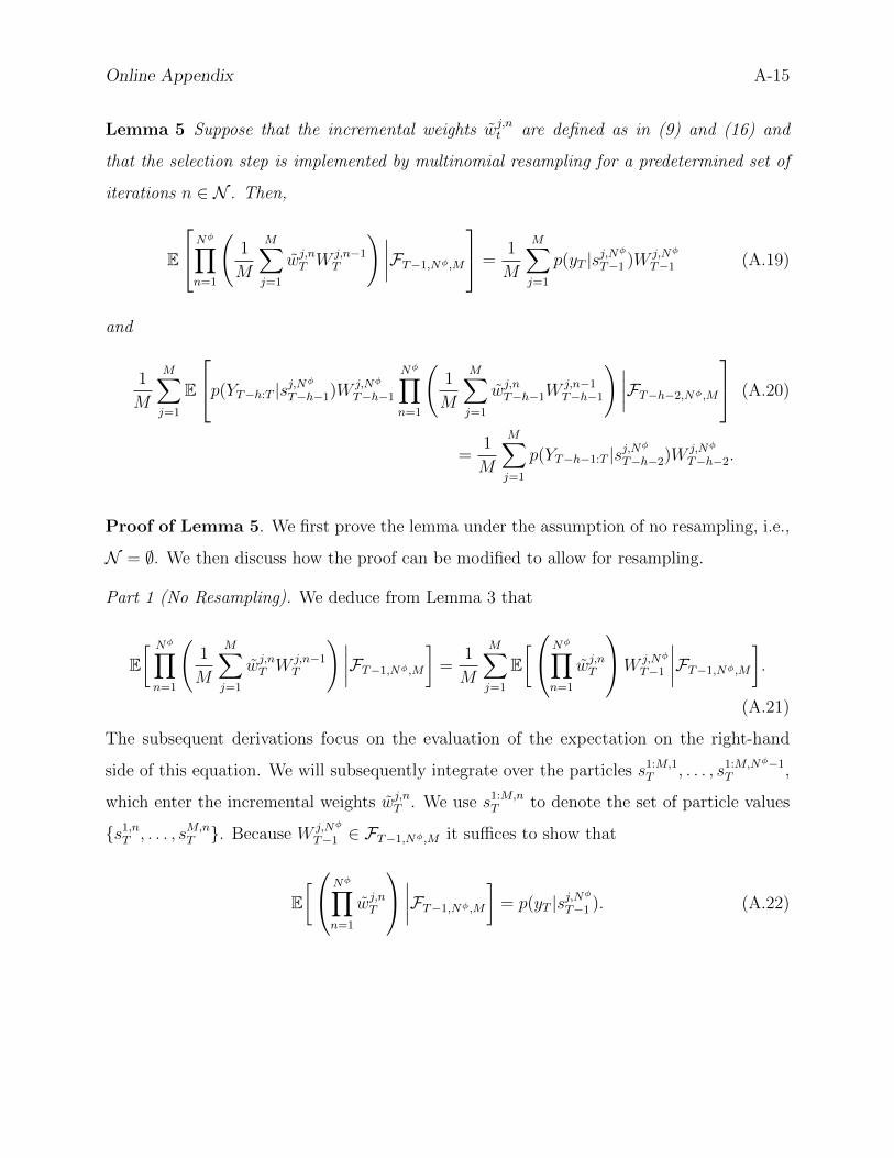
Online Appendix A-15
Lemma 5 Suppose that the incremental weights wj,nt are defined as in (9) and (16) and
that the selection step is implemented by multinomial resampling for a predetermined set of
iterations n ∈ N . Then,
E
Nφ∏n=1
(1
M
M∑j=1
wj,nT W j,n−1T
)∣∣∣∣FT−1,Nφ,M
=1
M
M∑j=1
p(yT |sj,Nφ
T−1 )W j,Nφ
T−1 (A.19)
and
1
M
M∑j=1
E
p(YT−h:T |sj,Nφ
T−h−1)W j,Nφ
T−h−1
Nφ∏n=1
(1
M
M∑j=1
wj,nT−h−1Wj,n−1T−h−1
)∣∣∣∣FT−h−2,Nφ,M
(A.20)
=1
M
M∑j=1
p(YT−h−1:T |sj,Nφ
T−h−2)W j,Nφ
T−h−2.
Proof of Lemma 5. We first prove the lemma under the assumption of no resampling, i.e.,
N = ∅. We then discuss how the proof can be modified to allow for resampling.
Part 1 (No Resampling). We deduce from Lemma 3 that
E[ Nφ∏n=1
(1
M
M∑j=1
wj,nT W j,n−1T
)∣∣∣∣FT−1,Nφ,M
]=
1
M
M∑j=1
E[Nφ∏
n=1
wj,nT
W j,Nφ
T−1
∣∣∣∣FT−1,Nφ,M
].
(A.21)
The subsequent derivations focus on the evaluation of the expectation on the right-hand
side of this equation. We will subsequently integrate over the particles s1:M,1T , . . . , s1:M,Nφ−1
T ,
which enter the incremental weights wj,nT . We use s1:M,nT to denote the set of particle values
{s1,nT , . . . , sM,n
T }. Because W j,Nφ
T−1 ∈ FT−1,Nφ,M it suffices to show that
E[Nφ∏
n=1
wj,nT
∣∣∣∣FT−1,Nφ,M
]= p(yT |sj,N
φ
T−1 ). (A.22)

Online Appendix A-16
Recall that the initial state particle sj,1T is generated from the state-transition equation
p(sT |sj,Nφ
T−1 ). The first incremental weight is defined as
wj,1T = p1(yT |sj,1T ).
The incremental weight in tempering iteration n is given by
wj,nT =pn(yT |sj,n−1
T )
pn−1(yT |sj,n−1T )
.
Because we are omitting the selection step, the new particle value is generated in the mutation
step by sampling from the Markov transition kernel
sj,nT ∼ Kn(snT |sj,n−1T , sj,N
φ
T−1 ), (A.23)
which has the invariance property
pn(sT |yT , sT−1) =
∫Kn(sT |sT ; sT−1)pn(sT |yT , sT−1)dsT . (A.24)
Using the previous notation, we can write
E
Nφ∏n=1
wj,nT
∣∣∣∣FT−1,Nφ,M
(A.25)
=
∫· · ·∫ Nφ∏
n=3
pn(yT |sj,n−1T )
pn−1(yT |sj,n−1T )
Kn−1(sj,n−1T |sj,n−2
T , sj,Nφ
T−1 )
×p2(yT |sj,1T )
p1(yT |sj,1T )p1(yT |sj,1T )p(sj,1T |sj,N
φ
T−1 )dsj,1T · · · dsj,Nφ−1
T .
The bridge posterior densities were defined as
pn(st|yt, st−1) =pn(yt|st)p(st|st−1)
pn(yt|st−1), pn(yt|st−1) =
∫pn(yt|st)p(st|st−1)dst. (A.26)

Online Appendix A-17
Using the invariance property of the transition kernel in (A.24) and the definition of the
bridge posterior densities, we deduce that
∫Kn−1(sj,n−1
T |sj,n−2T , sj,N
φ
T−1 )pn−1(yT |sj,n−2T )p(sj,n−2
T |sj,Nφ
T−1 )dsj,n−2T (A.27)
=
∫Kn−1(sj,n−1
T |sj,n−2T , sj,N
φ
T−1 )pn−1(sj,n−2T |yT , sj,N
φ
T−1 )pn−1(yT |sj,Nφ
T−1 )dsj,n−2T
= pn−1(sj,n−1T |yT , sj,N
φ
T−1 )pn−1(yT |sj,Nφ
T−1 )
= pn−1(yT |sj,n−1T )p(sj,n−1
T |sj,Nφ
T−1 ).
The first equality follows from Bayes Theorem in (A.26). The second equality follows from
the invariance property of the transition kernel. The third equality uses Bayes Theorem
again.
We can now evaluate the integrals in (A.25). Consider the terms involving sj,1T :
∫K2(sj,2T |sj,1T , sj,N
φ
T−1 )p2(yT |sj,1T )
p1(yT |sj,1T )p1(yT |sj,1T )p(sj,1T |sj,N
φ
T−1 )dsj,1T (A.28)
=
∫K2(sj,2T |sj,1T , sj,N
φ
T−1 )p2(yT |sj,1T )p(sj,1T |sj,Nφ
T−1 )dsj,1T
= p2(yT |sj,2T )p(sj,2T |sj,Nφ
T−1 ).
Thus,
E
Nφ∏n=1
wj,nT
∣∣∣∣FT−1,Nφ,M
(A.29)
=
∫· · ·∫ Nφ∏
n=4
pn(yT |sj,n−1T )
pn−1(yT |sj,n−1T )
Kn−1(sj,n−1T |sj,n−2
T , sj,Nφ
T−1 )
×p3(yT |sj,2T )
p2(yT |sj,2T )p2(yT |sj,2T )p(sj,2T |sj,N
φ
T−1 )dsj,2T · · · dsj,Nφ−1
T
=
∫pNφ(yT |sj,N
φ−1T )
pNφ−1(yT |sj,Nφ−1
T )pNφ−1(yT |sj,N
φ−1T )p(sj,N
φ−1T |sj,Nφ
T−1 )dsj,Nφ−1
T
= p(yT |sj,Nφ
T−1 ).

Online Appendix A-18
The first equality follows from (A.28). The second equality is obtained by sequentially
integrating out sj,2T , . . . , sj,Nφ−2
T , using a similar argument as for sj,1T . This proves the first
part of the lemma.
Part 2 (No Resampling). Using Lemma 3, we write
E[p(YT−h:T |sj,N
φ
T−h−1, θ)Wj,Nφ
T−h−1
Nφ∏n=1
(1
M
M∑j=1
wj,nT−h−1Wj,n−1T−h−1
)∣∣∣∣FT−h−2,Nφ,M
]
= E[p(YT−h:T |sj,N
φ
T−h−1, θ)
Nφ∏n=1
wj,nT−h−1
W j,Nφ
T−h−2
∣∣∣∣FT−h−2,Nφ,M
](A.30)
To prove the second part of the lemma, we slightly modify the last step of the integration
in (A.29):
E
p(YT−h:T |sj,Nφ
T−h−1)
Nφ∏n=1
wj,nT−h−1
∣∣∣∣FT−2,Nφ,M
(A.31)
=
∫p(YT−h:T |sj,N
φ
T−h−1)pNφ(yT−h−1|sj,Nφ−1
T−h−1)p(sj,Nφ−1
T−h−1 |sj,Nφ
T−h−2)dsj,Nφ−1
T−h−1
= p(YT−h−1:T |sj,Nφ
T−h−2),
as required.
Part 1 (Resampling in tempering iteration n). We now assume that the selection step is
executed once, in iteration n, i.e., N = {n}. For reasons that will become apparent subse-
quently, we will use i subscripts for particles in stages n = 1, . . . , n− 1. Using Lemma 3, we
deduce that it suffices to show:
E[( n−1∏
n=1
(1
M
M∑i=1
wi,nT W i,n−1T
))(1
M
M∑j=1
wj,nT W j,n−1T
)(A.32)
×(
1
M
M∑j=1
( Nφ∏n=n+1
wj,nT
)W j,nT
)∣∣∣∣FT−1,Nφ,M
]
=1
M
M∑j=1
p(yT |sj,Nφ
T−1 )W j,Nφ
T−1 .

Online Appendix A-19
To evaluate the expectation, we need to integrate over the particles s1:M,1T , . . . , s1:M,Nφ
T as well
as the particles s1:M,nT generated during the selection step. We have to distinguish two cases:
Case 1, n 6= n : sj,nT ∼ Kn(sj,nT |sj,n−1T , sj,N
φ
T ), j = 1, . . . ,M
Case 2, n = n : sj,nT ∼ Kn(sj,nT |sj,nT , sj,Nφ
T ), j = 1, . . . ,M ;
sj,nT ∼MN(s1:M,n−1T , W 1:M,n
T
), j = 1, . . . ,M
where MN(·) here denotes the multinomial distribution.
In a preliminary step, we are integrating out the particles s1:M,nT . These particles enter the
Markov transition kernel Kn(sj,nT |sj,nT , sj,Nφ
T−1 ) as well as the conditional density p(sj,nT |s1:M,n−1T ).
Under the assumption that the resampling step is executed using multinomial resampling,
p(sj,nT |s1:M,n−1T ) =
1
M
M∑i=1
W j,nT δ(sj,nT − si,n−1
T ),
where δ(x) is the Dirac function with the property that δ(x) = 0 for x 6= 0 and∫δ(x)dx = 1.
Integrating out the resampled particles yields
p(s1:M,nT |s1:M,n−1
T ) (A.33)
=
∫ M∏j=1
Kn(sj,nT |sj,nT , sj,Nφ
T−1 )
[1
M
M∑i=1
W i,nT δ(sj,nT − si,n−1
T )
]ds1:M,n
T
=M∏j=1
∫Kn(sj,nT |sj,nT , sj,N
φ
T−1 )
[1
M
M∑i=1
W i,nT δ(sj,nT − si,n−1
T )
]dsj,nT
=M∏j=1
[1
M
M∑i=1
W i,nT Kn(sj,nT |si,n−1
T , si,Nφ
T−1)
].
In the last equation, the superscript for sT−1 changes from j to i because during the resam-
pling, we keep track of the history of the particle. Thus, if for particle j = 1 the value s1,nT
is set to s3,n−1T , we also use s3,Nφ
T−1 for this particle.

Online Appendix A-20
We can now express the expected value, which we abbreviate as E , as the following
integral:
E = E[( n−1∏
n=1
(1
M
M∑i=1
wi,nT W i,n−1T−1
))(1
M
M∑j=1
wj,nT W j,n−1T
)(A.34)
×(
1
M
M∑j=1
( Nφ∏n=n+1
wj,nT
)W j,nT
)∣∣∣∣FT−1,Nφ,M
]
=
∫· · ·∫ ( n−1∏
n=1
(1
M
M∑i=1
wi,nT W i,n−1T−1
))(1
M
M∑j=1
wj,nT W j,n−1T
)(1
M
M∑j=1
( Nφ∏n=n+1
wj,nT
))
×( n−1∏n=1
M∏j=1
Kn(si,nT |si,n−1T , si,N
φ
T−1)
)( M∏j=1
[1
M
M∑i=1
W i,nT Kn(sj,nT |si,n−1
T , si,Nφ
T−1)
])
×( Nφ−1∏n=n+1
M∏j=1
Kn(sj,nT |sj,n−1T , sj,N
φ
T−1 )
)ds1:M,1
T · · · ds1:M,Nφ−1T .
For the second equality, we used the fact that W j,nT = 1.
Using Lemma 4, we can write
∫· · ·∫ (
1
M
M∑j=1
( Nφ∏n=n+1
wj,nT
)( Nφ−1∏n=n+1
M∏j=1
Kn(sj,nT |sj,n−1T , sj,N
φ
T−1 )
)ds1:M,n+1
T · · · ds1:M,Nφ−1T
=1
M
M∑j=1
∫· · ·∫ ( Nφ∏
n=n+1
wj,nT
)( Nφ−1∏n=n+1
Kn(sj,nT |sj,n−1T , sj,N
φ
T−1 )
)dsj,n+1
T · · · dsj,Nφ−1T
=1
M
M∑j=1
F (sj,nT , sj,Nφ
T−1 ). (A.35)
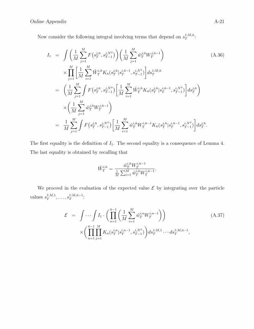
Online Appendix A-21
Now consider the following integral involving terms that depend on s1:M,nT :
I1 =
∫ (1
M
M∑j=1
F(sj,nT , sj,N
φ
T−1
))( 1
M
M∑j=1
wj,nT W j,n−1T
)(A.36)
×M∏j=1
[1
M
M∑i=1
W i,nT Kn(sj,nT |si,n−1
T , si,Nφ
T−1)
]ds1:M,n
T
=
(1
M
M∑j=1
∫F(sj,nT , sj,N
φ
T−1
)[ 1
M
M∑i=1
W i,nT Kn(sj,nT |si,n−1
T , si,Nφ
T−1)
]dsj,nT
)
×(
1
M
M∑j=1
wj,nT W j,n−1T
)
=1
M
M∑j=1
∫F(sj,nT , sj,N
φ
T−1
)[ 1
M
M∑i=1
wi,nT W i,n−1T Kn(sj,nT |si,n−1
T , si,Nφ
T−1)
]dsj,nT .
The first equality is the definition of I1. The second equality is a consequence of Lemma 4.
The last equality is obtained by recalling that
W i,nT =
wi,nT W i,n−1T
1M
∑Mi=1 w
i,nT W i,n−1
T
.
We proceed in the evaluation of the expected value E by integrating over the particle
values s1:M,1T , . . . , s1:M,n−1
T :
E =
∫· · ·∫I1 ·( n−1∏n=1
(1
M
M∑i=1
wi,nT W i,n−1T
))(A.37)
×( n−1∏n=1
M∏j=1
Kn(si,nT |si,n−1T , si,N
φ
T−1)
)ds1:M,1
T · · · ds1:M,n−1T ,

Online Appendix A-22
where
I1 ·( n−1∏n=1
(1
M
M∑i=1
wi,nT W i,n−1T
))
=
(1
M
M∑j=1
∫F(sj,nT , sj,N
φ
T−1
)[ 1
M
M∑i=1
wi,nT W i,n−1T Kn(sj,nT |si,n−1
T , si,Nφ
T−1)
]dsj,nT
)
×( n−1∏n=1
(1
M
M∑i=1
wi,nT W i,n−1T
))
=1
M
M∑j=1
∫F(sj,nT , sj,N
φ
T−1
)[ 1
M
M∑i=1
wi,nT W i,n−1T
( n−1∏n=1
(1
M
M∑i=1
wi,nT W i,n−1T
))×Kn(sj,nT |si,n−1
T , si,Nφ
T−1)
]dsj,nT
=1
M
M∑j=1
∫F(sj,nT , sj,N
φ
T−1
)[ 1
M
M∑i=1
wi,nT
( n−1∏n=1
wi,nT
)W i,Nφ
T−1
×Kn(sj,nT |si,n−1T , si,N
φ
T−1)
]dsj,nT .
The last equality follows from the second part of Lemma 3. Notice the switch from j to i
superscript for functions of particles in stages n < n. Thus,
E =1
M
M∑j=1
∫F(sj,nT , sj,N
φ
T−1
) ∫· · ·∫ [
1
M
M∑i=1
wi,nT
( n−1∏n=1
wi,nT
)W i,Nφ
T−1 (A.38)
×Kn(sj,nT |si,n−1T , si,N
φ
T−1)
]( n−1∏n=1
M∏i=1
Kn(si,nT |si,n−1T , si,N
φ
T−1)
)ds1:M,1
T · · · ds1:M,n−1T dsj,nT
=1
M
M∑j=1
∫F(sj,nT , sj,N
φ
T−1
)[ 1
M
M∑i=1
∫· · ·∫ ( n∏
n=1
wi,nT
)W i,Nφ
T−1
×Kn(sj,nT |si,n−1T , si,N
φ
T−1)n−1∏n=1
Kn(si,nT |si,n−1T , si,N
φ
T−1)dsi,1T · · · dsi,n−1T
]dsj,nT .
The second equality follows from Lemma 4. The calculations in (A.29) imply that
∫· · ·∫ ( n∏
n=1
wi,nT
)W i,Nφ
T−1
n−1∏n=1
Kn(si,nT |si,n−1T , si,N
φ
T−1)dsi,1T · · · dsi,n−2T (A.39)
= pn−1(yT |si,n−1T )p(si,n−1
T |si,Nφ
T−1)W i,Nφ
T−1 .

Online Appendix A-23
In turn,
E =1
M
M∑j=1
∫F(sj,nT , sj,N
φ
T−1
)[ 1
M
M∑i=1
∫Kn(sj,nT |si,n−1
T , si,Nφ
T−1)
×pn(yT |si,n−1T )p(si,n−1
T |si,Nφ
T−1)W i,Nφ
T−1 dsi,n−1T
]dsj,nT
=1
M
M∑i=1
[1
M
M∑j=1
∫F(sj,nT , sj,N
φ
T−1
)Kn(sj,nT |si,n−1
T , si,Nφ
T−1)dsj,nT (A.40)
×pn(yT |si,n−1T )p(si,n−1
T |si,Nφ
T−1)W i,Nφ
T−1 dsi,n−1T
]=
1
M
M∑i=1
∫F(si,nT , s
i,Nφ
T−1
)pn(yT |si,nT )p(si,nT |si,N
φ
T−1)W i,Nφ
T−1 dsi,nT
=1
M
M∑j=1
∫· · ·∫ ( Nφ∏
n=n+1
wj,nT
)( Nφ−1∏n=n+1
Kn(sj,nT |sj,n−1T , sj,N
φ
T−1 )
)×pn(yT |sj,nT )p(sj,nT |sj,N
φ
T−1 )W j,Nφ
T−1 dsj,n+1T · · · dsj,Nφ−1
T pn(yT |sj,nT )p(sj,nT |sj,Nφ
T−1 )dsj,nT
=1
M
M∑j=1
p(yT |sj,Nφ
T−1 )W j,Nφ
T−1 .
The second equality is obtained by changing the order of two summations. To obtain the
third equality, we integrate out the si,n−1T terms along the lines of (A.27). Notice that the
value of the integral is identical for all values of the j superscript. Thus, we simply set j = i
and drop the average. For the fourth equality, we plug in the definition of F(si,nT , s
i,Nφ
T−1
)and
replace the i index with a j index. The last equality follows from calculations similar to
those in (A.29). This completes the analysis of Part 1.
Part 2 (Resampling in tempering iteration n). A similar argument as for Part 1 can be used
to extend the result for Part 2.
Resampling in multiple tempering iterations. The previous analysis can be extended to the
case in which the selection step is executed in multiple tempering iterations n ∈ N , assuming
that the set N does not itself depend on the particle system. �

Online Appendix A-24
A.3.2 Proof of Main Theorem
Proof of Theorem 2. Suppose that for any h such that 0 ≤ h ≤ T − 1
E[p(YT−h:T |Y1:T−h−1, θ)|FT−h−1,Nφ,M
]=
1
M
M∑j=1
p(YT−h:T |sj,Nφ
T−h−1, θ)Wj,Nφ
T−h−1, (A.41)
where
p(YT−h:T |Y1:T−h−1, θ) =T∏
t=T−h
Nφ∏n=1
(1
M
M∑j=1
wj,nt W j,n−1t
) .
Then, by setting h = T − 1, we can deduce that
E[p(Y1:T |θ)|F0,Nφ,M
]=
1
M
M∑j=1
p(Y1:T |sj,Nφ
0 , θ)W j,Nφ
0 . (A.42)
Recall that for period t = 0, we adopted the convention that Nφ = 1 and assumed that the
states were initialized by direct sampling: sj,Nφ
0 ∼ p(s0) and W j,Nφ
0 = 1. Thus,
E[p(Y1:T |θ)
]= E
[E[p(Y1:T |θ)|F0,Nφ,M
]](A.43)
= E[
1
M
M∑j=1
p(Y1:T |sj,Nφ
0 , θ)W j,Nφ
0
]=
∫p(Y1:T |s0, θ)p(s0)ds0
= p(Y1:T |θ),
as desired.
In the remainder of the proof, we use an inductive argument to establish (A.41). If (A.41)

Online Appendix A-25
holds for h, it also has to hold for h+ 1:
E[p(YT−h−1:T |Y1:T−h−2, θ)|FT−h−2,Nφ,M
]= E
[E[p(YT−h:T |Y1:T−h−1, θ)
∣∣FT−h−1,Nφ,M
]p(yT−h−1|Y1:T−h−2, θ)
∣∣∣∣FT−h−2,Nφ,M
]=
1
M
M∑j=1
E[p(YT−h:T |sj,N
φ
T−h−1, θ)Wj,Nφ
T−h−1p(yT−h−1|Y1:T−h−2, θ)∣∣FT−h−2,Nφ,M
]=
1
M
M∑j=1
E
p(YT−h:T |sj,Nφ
T−h−1, θ)Wj,Nφ
T−h−1
Nφ∏n=1
(1
M
M∑j=1
wj,nT−h−1Wj,n−1T−h−1
)∣∣∣∣FT−h−2,Nφ,M
=
1
M
M∑j=1
p(YT−h−1:T |sj,Nφ
T−h−2, θ)Wj,Nφ
T−h−2.
Note that FT−h−2,Nφ,M ⊂ FT−h−1,Nφ,M . Thus, the first equality follows from the law of
iterated expectations. The second equality follows from the inductive hypothesis (A.41).
The third equality uses the definition of the period-likelihood approximation in (23) of Al-
gorithm 2. The last equality follows from the second part of Lemma 5.
We now verify that the inductive hypothesis (A.41) holds for h = 0. Using the definition
of p(yT |Y1:T−1, θ), we can write
E[p(yT |Y1:T−1, θ)|FT−1,Nφ,M
]= E
Nφ∏n=1
(1
M
M∑j=1
wj,nT W j,n−1T
)∣∣∣∣FT−1,Nφ,M
(A.44)
=1
M
M∑j=1
p(yT |sj,Nφ
T−1 )W j,Nφ
T−1 .
The second equality follows from the first part of Lemma 5. Thus, we can deduce that (A.41)
holds for h = T − 1 as required. This completes the proof. �

Online Appendix A-26
B DSGE Models and Data Sources
B.1 Small-Scale DSGE Model
B.1.1 Equilibrium Conditions
We write the equilibrium conditions by expressing each variable in terms of percentage
deviations from its steady state value. Let xt = ln(xt/x) and write
1 = βEt[e−τ ct+1+τ ct+Rt−zt+1−πt+1
](A.45)
0 =(eπt − 1
) [(1− 1
2ν
)eπt +
1
2ν
](A.46)
−βEt[(eπt+1 − 1
)e−τ ct+1+τ ct+yt+1−yt+πt+1
]+
1− ννφπ2
(1− eτ ct
)ect−yt = e−gt − φπ2g
2
(eπt − 1
)2(A.47)
Rt = ρRRt−1 + (1− ρR)ψ1πt (A.48)
+(1− ρR)ψ2 (yt − gt) + εR,t
gt = ρggt−1 + εg,t (A.49)
zt = ρz zt−1 + εz,t. (A.50)
Log-linearization and straightforward manipulation of Equations (A.45) to (A.47) yield
the following representation for the consumption Euler equation, the New Keynesian Phillips
curve, and the monetary policy rule:
yt = Et[yt+1]− 1
τ
(Rt − Et[πt+1]− Et[zt+1]
)(A.51)
+gt − Et[gt+1]
πt = βEt[πt+1] + κ(yt − gt)
Rt = ρRRt−1 + (1− ρR)ψ1πt + (1− ρR)ψ2 (yt − gt) + εR,t

Online Appendix A-27
where
κ = τ1− ννπ2φ
. (A.52)
To construct a likelihood function, we have to relate the model variables to a set of ob-
servables yt. We use the following three observables for estimation: quarter-to-quarter per
capita GDP growth rates (YGR), annualized quarter-to-quarter inflation rates (INFL), and
annualized nominal interest rates (INT). The three series are measured in percentages, and
their relationship to the model variables is given by the following set of equations:
Y GRt = γ(Q) + 100(yt − yt−1 + zt) (A.53)
INFLt = π(A) + 400πt
INTt = π(A) + r(A) + 4γ(Q) + 400Rt.
The parameters γ(Q), π(A), and r(A) are related to the steady states of the model economy
as follows:
γ = 1 +γ(Q)
100, β =
1
1 + r(A)/400, π = 1 +
π(A)
400.
The structural parameters are collected in the vector θ. Since in the first-order approximation
the parameters ν and φ are not separately identifiable, we express the model in terms of κ,
defined in (A.52). Let
θ = [τ, κ, ψ1, ψ2, ρR, ρg, ρz, r(A), π(A), γ(Q), σR, σg, σz]
′.
B.1.2 Data Sources
1. Per Capita Real Output Growth Take the level of real gross domestic product,
(FRED mnemonic “GDPC1”), call it GDPt. Take the quarterly average of the Civilian
Non-institutional Population (FRED mnemonic “CNP16OV” / BLS series “LNS10000000”),
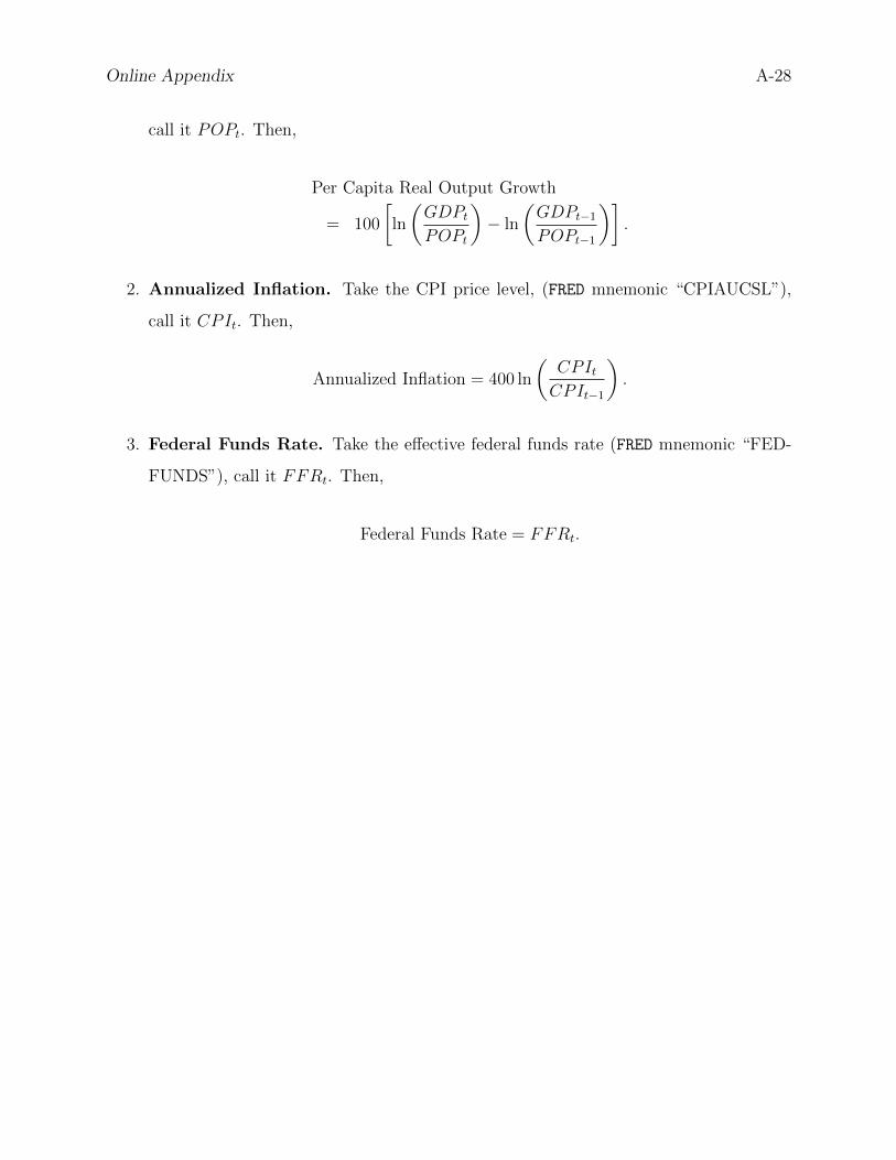
Online Appendix A-28
call it POPt. Then,
Per Capita Real Output Growth
= 100
[ln
(GDPtPOPt
)− ln
(GDPt−1
POPt−1
)].
2. Annualized Inflation. Take the CPI price level, (FRED mnemonic “CPIAUCSL”),
call it CPIt. Then,
Annualized Inflation = 400 ln
(CPItCPIt−1
).
3. Federal Funds Rate. Take the effective federal funds rate (FRED mnemonic “FED-
FUNDS”), call it FFRt. Then,
Federal Funds Rate = FFRt.

Online Appendix A-29
B.2 The Smets-Wouters Model
B.2.1 Equilibrium Conditions
The log-linearized equilibrium conditions of the Smets and Wouters (2007) model take the
following form:
yt = cy ct + iy it + zyzt + εgt (A.54)
ct =h/γ
1 + h/γct−1 +
1
1 + h/γEtct+1 (A.55)
+wlc(σc − 1)
σc(1 + h/γ)(lt − Etlt+1)
− 1− h/γ(1 + h/γ)σc
(rt − Etπt+1)− 1− h/γ(1 + h/γ)σc
εbt
it =1
1 + βγ(1−σc)it−1 +
βγ(1−σc)
1 + βγ(1−σc)Etit+1 (A.56)
+1
ϕγ2(1 + βγ(1−σc))qt + εit
qt = β(1− δ)γ−σcEtqt+1 − rt + Etπt+1 (A.57)
+(1− β(1− δ)γ−σc)Etrkt+1 − εbtyt = Φ(αkst + (1− α)lt + εat ) (A.58)
kst = kt−1 + zt (A.59)
zt =1− ψψ
rkt (A.60)
kt =(1− δ)γ
kt−1 + (1− (1− δ)/γ)it (A.61)
+(1− (1− δ)/γ)ϕγ2(1 + βγ(1−σc))εit
µpt = α(kst − lt)− wt + εat (A.62)
πt =βγ(1−σc)
1 + ιpβγ(1−σc)Etπt+1 +
ιp1 + βγ(1−σc)
πt−1 (A.63)
− (1− βγ(1−σc)ξp)(1− ξp)(1 + ιpβγ(1−σc))(1 + (Φ− 1)εp)ξp
µpt + εpt

Online Appendix A-30
rkt = lt + wt − kst (A.64)
µwt = wt − σl lt −1
1− h/γ (ct − h/γct−1) (A.65)
wt =βγ(1−σc)
1 + βγ(1−σc)(Etwt+1 (A.66)
+Etπt+1) +1
1 + βγ(1−σc)(wt−1 − ιwπt−1)
−1 + βγ(1−σc)ιw1 + βγ(1−σc)
πt
− (1− βγ(1−σc)ξw)(1− ξw)
(1 + βγ(1−σc))(1 + (λw − 1)εw)ξwµwt + εwt
rt = ρrt−1 + (1− ρ)(rππt + ry(yt − y∗t )) (A.67)
+r∆y((yt − y∗t )− (yt−1 − y∗t−1)) + εrt .
The exogenous shocks evolve according to
εat = ρaεat−1 + ηat (A.68)
εbt = ρbεbt−1 + ηbt (A.69)
εgt = ρgεgt−1 + ρgaη
at + ηgt (A.70)
εit = ρiεit−1 + ηit (A.71)
εrt = ρrεrt−1 + ηrt (A.72)
εpt = ρrεpt−1 + ηpt − µpηpt−1 (A.73)
εwt = ρwεwt−1 + ηwt − µwηwt−1. (A.74)

Online Appendix A-31
The counterfactual no-rigidity prices and quantities evolve according to
y∗t = cy c∗t + iy i
∗t + zyz
∗t + εgt (A.75)
c∗t =h/γ
1 + h/γc∗t−1 +
1
1 + h/γEtc∗t+1 (A.76)
+wlc(σc − 1)
σc(1 + h/γ)(l∗t − Etl∗t+1)
− 1− h/γ(1 + h/γ)σc
r∗t −1− h/γ
(1 + h/γ)σcεbt
i∗t =1
1 + βγ(1−σc)i∗t−1 +
βγ(1−σc)
1 + βγ(1−σc)Eti∗t+1
+1
ϕγ2(1 + βγ(1−σc))q∗t + εit (A.77)
q∗t = β(1− δ)γ−σcEtq∗t+1 − r∗t (A.78)
+(1− β(1− δ)γ−σc)Etrk∗t+1 − εbty∗t = Φ(αks∗t + (1− α)l∗t + εat ) (A.79)
ks∗t = k∗t−1 + z∗t (A.80)
z∗t =1− ψψ
rk∗t (A.81)
k∗t =(1− δ)γ
k∗t−1 + (1− (1− δ)/γ)it (A.82)
+(1− (1− δ)/γ)ϕγ2(1 + βγ(1−σc))εit
w∗t = α(ks∗t − l∗t ) + εat (A.83)
rk∗t = l∗t + w∗t − k∗t (A.84)
w∗t = σl l∗t +
1
1− h/γ (c∗t + h/γc∗t−1). (A.85)

Online Appendix A-32
The steady state (ratios) that appear in the measurement equation or the log-linearized
equilibrium conditions are given by
γ = γ/100 + 1 (A.86)
π∗ = π/100 + 1 (A.87)
r = 100(β−1γσcπ∗ − 1) (A.88)
rkss = γσc/β − (1− δ) (A.89)
wss =
(αα(1− α)(1−α)
Φrkssα
) 11−α
(A.90)
ik = (1− (1− δ)/γ)γ (A.91)
lk =1− αα
rksswss
(A.92)
ky = Φl(α−1)k (A.93)
iy = (γ − 1 + δ)ky (A.94)
cy = 1− gy − iy (A.95)
zy = rkssky (A.96)
wlc =1
λw
1− αα
rksskycy
. (A.97)
The measurement equations take the form:
Y GRt = γ + yt − yt−1 (A.98)
INFt = π + πt
FFRt = r + Rt
CGRt = γ + ct − ct−1
IGRt = γ + it − it−1
WGRt = γ + wt − wt−1
HOURSt = l + lt.

Online Appendix A-33
B.2.2 Data
The data cover 1966Q1 to 2004Q4. The construction follows that of Smets and Wouters
(2007). Output data come from the NIPA; other sources are noted in the exposition.
1. Per Capita Real Output Growth. Take the level of real gross domestic prod-
uct (FRED mnemonic “GDPC1”), call it GDPt. Take the quarterly average of the
Civilian Non-institutional Population (FRED mnemonic “CNP16OV” and BLS series
“LNS10000000”) normalized so that its 1992Q3 value is 1 and call it POPt. Then,
Per Capita Real Output Growth
= 100
[ln
(GDPtPOPt
)− ln
(GDPt−1
POPt−1
)].
2. Per Capita Real Consumption Growth. Take the level of personal consumption
expenditures (FRED mnemonic “PCEC”), call it CONSt. Take the level of the GDP
price deflator (FRED mnemonic “GDPDEF”) and call it GDPPt. Then,
Per Capita Real Consumption Growth
= 100
[ln
(CONSt
GDPPtPOPt
)− ln
(CONSt−1
GDPPt−1POPt−1
)].
3. Per Capita Real Investment Growth. Take the level of fixed private investment
(FRED mnemonic “FPI”) and call it INVt. Then,
Per Capita Real Investment Growth
= 100
[ln
(INVt
GDPPtPOPt
)− ln
(INVt−1
GDPPt−1POPt−1
)].
4. Per Capita Real Wage Growth. Take the BLS measure of compensation per
hour for the nonfarm business sector (FRED mnemonic “COMPNFB” / BLS series

Online Appendix A-34
“PRS85006103”) and call it Wt. Then,
Per Capita Real Wage Growth
= 100
[ln
(Wt
GDPPt
)− ln
(Wt−1
GDPPt−1
)].
5. Per Capita Hours Index. Take the index of average weekly nonfarm business hours
(FRED mnemonic / BLS series “PRS85006023”) and call it HOURSt. Take the number
of employed civilians (FRED mnemonic “CE16OV”), normalized so that its 1992Q3 value
is 1 and call it EMPt. Then,
Per Capita Hours = 100 ln
(HOURStEMPt
POPt
).
The series is then demeaned.
6. Inflation. Take the GDP price deflator, then
Inflation = 100 ln
(GDPPtGDPPt−1
).
7. Federal Funds Rate. Take the effective federal funds rate (FRED mnemonic “FED-
FUNDS”) and call it FFRt. Then,
Federal Funds Rate = FFRt/4.

Online Appendix A-35
C Computational Details
The code for this project is available at http://github.com/eph/tempered_pf. The appli-
cations in Section 4 were coded in Fortran and compiled using the Intel Fortran Compiler
(version: 13.0.0), including the math kernel library. The calculations in Algorithm 1, part
2(a)ii, Algorithm 2, part 1(a)i, and Algorithm 2, part 2(c) were implemented using OpenMP
(shared memory) multithreading.

Online Appendix A-36
D Additional Numerical Results
D.1 Filtered States for Small-Scale DSGE Model
To document the accuracy of the filtered state, we consider the latent government spending
shock as a prototypical hidden state. Using the Kalman filter, we can compute E[gt|Y1:T ],
which we compare to the particle filter approximation, denoted by E[gt|Y1:T ]. Figure A-1 plots
root-mean-squared errors (RMSEs) for E[gt|Y1:T ]. The ranking of the filters is consistent with
the ranking based on the accuracy of the likelihood approximations. The BSPF performs
the worst. Using the TPF with M = 40, 000 particles reduces the RMSE roughly by a factor
of three.
Figure A-1: Small-Scale Model: Accuracy of Filtered State
1984 1989 1994 19990.0
0.5
1.0
1.5
2.0
2.5
3.0
3.5
BSPF, M=40kTPF(r*=2), M=40kTPF(r*=3), M=40k
TPF(r*=2), M=4kTPF(r*=3), M=4k
Notes: The figure depicts RMSEs associated with E[gt|Y1:t]. Results are based on Nrun = 100independent runs of the particle filters.
D.2 Smets-Wouters Model
The parameters used for the likelihood evaluation of the SW model are summarized in
Table A-1.
In Table A-2 we report the accuracy statistics for the TPF with NMH = 1. Holding the
number of particles fixed at M = 40, 000 and reducing the number of mutation steps from
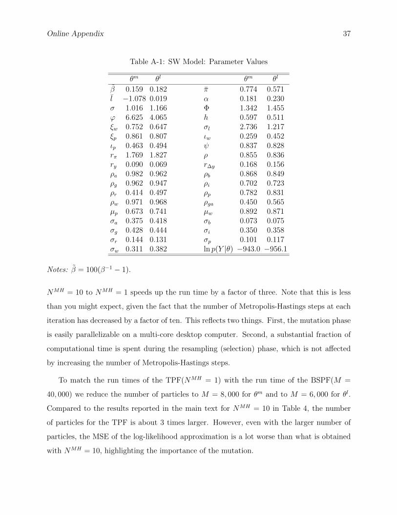
Online Appendix 37
Table A-1: SW Model: Parameter Values
θm θl θm θl
β 0.159 0.182 π 0.774 0.571l −1.078 0.019 α 0.181 0.230σ 1.016 1.166 Φ 1.342 1.455ϕ 6.625 4.065 h 0.597 0.511ξw 0.752 0.647 σl 2.736 1.217ξp 0.861 0.807 ιw 0.259 0.452ιp 0.463 0.494 ψ 0.837 0.828rπ 1.769 1.827 ρ 0.855 0.836ry 0.090 0.069 r∆y 0.168 0.156ρa 0.982 0.962 ρb 0.868 0.849ρg 0.962 0.947 ρi 0.702 0.723ρr 0.414 0.497 ρp 0.782 0.831ρw 0.971 0.968 ρga 0.450 0.565µp 0.673 0.741 µw 0.892 0.871σa 0.375 0.418 σb 0.073 0.075σg 0.428 0.444 σi 0.350 0.358σr 0.144 0.131 σp 0.101 0.117σw 0.311 0.382 ln p(Y |θ) −943.0 −956.1
Notes: β = 100(β−1 − 1).
NMH = 10 to NMH = 1 speeds up the run time by a factor of three. Note that this is less
than you might expect, given the fact that the number of Metropolis-Hastings steps at each
iteration has decreased by a factor of ten. This reflects two things. First, the mutation phase
is easily parallelizable on a multi-core desktop computer. Second, a substantial fraction of
computational time is spent during the resampling (selection) phase, which is not affected
by increasing the number of Metropolis-Hastings steps.
To match the run times of the TPF(NMH = 1) with the run time of the BSPF(M =
40, 000) we reduce the number of particles to M = 8, 000 for θm and to M = 6, 000 for θl.
Compared to the results reported in the main text for NMH = 10 in Table 4, the number
of particles for the TPF is about 3 times larger. However, even with the larger number of
particles, the MSE of the log-likelihood approximation is a lot worse than what is obtained
with NMH = 10, highlighting the importance of the mutation.

Online Appendix 38
Table A-2: SW Model: PF Summary Statistics
BSPF TPFTarget Ineff. Ratio r∗ 2 3 2 3
High Posterior Density: θ = θm
Number of Particles M 40,000 8,000 8,000 40,000 40,000
MSE(∆) 63,881.68 11,349.01 18,676.99 3,858.63 5,911.39
Bias(∆) -245.64 -100.65 -128.98 -57.71 -72.92
Variance(∆) 3,543.79 1,219.55 2,041.44 527.94 594.46
T−1∑T
t=1 Nφ,t 1.00 6.17 4.75 6.13 4.72Average Run Time (sec) 3.33 3.97 3.01 22.41 17.54
Low Posterior Density: θ = θl
Number of Particles M 40,000 6,000 6,000 40,000 40,000
MSE(∆) 69,612.88 22,052.28 30,372.77 5,578.91 7,155.54
Bias(∆) -255.06 -142.43 -167.17 -71.37 -80.58
Variance(∆) 4,559.09 1,766.12 2,426.31 485.38 661.68
T−1∑T
t=1 Nφ,t 1.00 6.26 4.81 6.22 4.77Average Run Time (sec) 3.28 3.35 2.35 22.69 18.19
Notes: Results are based on Nrun = 100 independent runs of the particle filters and NMH =1. The log likelihood discrepancy is defined as ∆ = ln p(Y1:T |θ)− ln p(Y1:T |θ).

Frank Schorfheide
Professor of Economics
University of Pennsylvania
July 21, 2017
Dr. Sylvia Kaufmann
Journal of Econometrics, Guest Editor
Study Center Gerzensee
VIA EMAIL
RE: Revision Tempered Particle Filtering
Dear Sylvia:
We are very grateful for the conditional acceptance of our paper Tempered Particle Filtering
in the special issue of the Journal of Econometrics. Many thanks for your careful reading of
the draft and your suggestions on how to improve the manuscript.
We reduced the length of the paper from 41 pages to 34 pages (keeping the formatting
the same). Foremost, the reduction was achieved by moving some material from the theory
section (Section 3) as well as some tables and figures from the empirical section (Section 4)
into the Online Appendix. We also condensed the exposition throughout the manuscript. In
response to your specific comments, here is what we did.
Notation:
1. We now make use of t subscripts, writing φn,t and Nφ,t, except in parts where the
notation gets too cumbersome or where it is assumed that the tempering schedule is
fixed (Section 3).
2. We removed the M subscripts.
3. We re-wrote the description of Algorithm 2. In particular, we changed the termination
condition to φn,t = 1 as you suggested and re-wrote/re-formatted Step 1(a)iii, which
describes when the do-loop is terminated.
Typos:
1. We corrected the typos flagged in line items 1. – 10.

Online Appendix 2
11. We harmonized the use of the h(·) notation with and without arguments.
12. Lemma 1: we now refer to the first Monte Carlo average as h1t|t−1, emphasizing that
this is an expectation given t−1 information. We also explicitly write in Lemma 2 that
the convergence results hold for n ≥ 2. The main issue is that the order of correction,
selection, and mutation is slightly different for n = 1.
13. We removed the ratio on the left-hand-side (it was essentially a labeling of the Monte
Carlo average). The notation did not look particularly nice and it was not used else-
where in the paper.
14. Done.
15. We fixed the notation. We meant to use A(1)2 to denote the first derivative of A2 with
respect to φn.
Finally, we adjusted the number of particles in columns 3 and 4 of Tables 2, 3, and 4 to
approximately equalize the run times of the TPFs and the BSPF(M = 40, 000). We feel
that the suggested edits led to an improved exposition and hope that we addressed your
comments in a satisfactory manner.
With best wishes,
Edward Herbst
Frank Schorfheide