RESEARCH ARTICLE

Temperature and evaporative water loss of leaf-sitting frogs therole of reflection spectraFrancisco Herrerıas-Azcue Chris Blount and Mark Dickinson

ABSTRACTThe near infrared reflection peak in some frogs has been speculatedto be either for enhancing crypticity or to help them withthermoregulation The theoretical background for the thermoregulatoryprocesses has been established before but little consideration hasbeen given to the contribution from the frogsrsquo reflection spectradifferences In this investigation the reflection spectra from a rangeof different species of frogs were taken and combined with precisesurface area measurements of frogs and an approximation to themass transfer coefficient of agar frogmodels Thesewere then used tosimulate the temperature and water evaporation in anurans with andwithout the near infrared reflective peak We have shown that thepresence of the near infrared reflection peak can contributesignificantly to the temperature and evaporative water loss of a frogThe significance of the steady-state temperature differences betweenfrogs with and without the near infrared reflection peak is discussed ina realistic and an extreme scenario Temperature differences of up to32degC were found and the rehydration period was increased by up to167 although this does not reduce the number of rehydrationevents between dawn and dusk

KEY WORDS Frogs Thermoregulation Reflection InfraredModelling Spectrum

INTRODUCTIONSince the discovery of pterorhodin in the skin of Agalychnisdachnicolor (formerly Pachymedusa dachnicolor) (Emerson et al1990) which replaces melanin and produces a characteristic peak inthe near infrared (NIR) part of the reflection spectrum the relevanceof NIR-enhanced reflection on different frog species has been anopen questionThe leaves these frogs often sit on also show a reflective peak in

the near infrared similar to that from frogs containing pterorhodinwhich would suggest that crypticity plays an important role(Schwalm et al 1977) However there are no reports of leaf-sitting frog predators that can see in that part of the spectrum whichmakes IR crypticity seemingly unimportantA reduction in the amount of light absorbed by an animal will

decrease the amount of energy gained and therefore there could be alink to thermoregulation Emerson et al (1990) briefly mention an

estimated 2degC temperature difference between frogs with andwithout NIR-enhanced reflectance but they only use a very roughcalculation and only take a single absorptance difference Here wereport on a detailed program to simulate the thermoregulatoryprocesses in frogs taking into account the reflection spectradifferences to analyse whether there is in fact a temperaturedifference and how it could reflect on the water balance of the frog

SIMULATION RESULTSFully exposed horizontal frogAn example of the output generated for a fully exposed horizontalfrog is shown in Fig 1 Note the scale of the temperature as well asthe shape of the temperature profile

In this scenario the C craspedopus reached a maximumtemperature of 283degC the black frog reached a maximum of305degC and the black IR-reflecting frog reached 277degC (the lattertwo are taken from separate simulations not shown in Fig 1) Whenrun for different frog species the difference between the highest andlowest maximum temperatures was 17degC

The mass of the frog versus time of day is shown in Fig 2 whereit can be seen that a completely black frog would need to rehydrateafter about 43 h of sun exposure whereas the black IR-reflectingfrog would need rehydration after 54 h The difference between themaximum exposure times before rehydration in real spectrasimulations was 06 h

Partially occluded frogAn example of the output generated for a partially occluded frog isshown in Fig 3 Note the scale of the temperature as well as theshape of the temperature profile and how this differs to that in Fig 1The shape is mainly due to the projected area of the frog changingthroughout the day

In this scenario the maximum temperature of the Cruziohylacalcarifer frog was 250degC for the black frog 255degC and for theblack IR-reflecting frog 247degCWhen run for different frog speciesthe difference between the highest and lowest maximumtemperatures was 05degC Fig 4 shows the temperature profile forall seven frogs used in the simulation

The shape of the temperature profile for all the frogs modelled areclearly very similar and at dawn and dusk they can all be seen toconverge to the same point as no solar radiation is being absorbed

In this scenario a completely black frog would need to rehydrateafter about 59 h and the black IR-reflecting frog would needrehydration after 68 h In the case of the real frogs the timedifference between the maximum exposure times before rehydrationis necessary was 06 h

DISCUSSIONAs can be seen in Fig 4 the temperature of the completelyabsorbing frog (black) and the one built to absorb all but the nearinfrared light (black IR-reflecting) serve as an envelope to theReceived 4 August 2016 Accepted 25 October 2016

Photon Science Institute School of Physics and Astronomy The University ofManchester Manchester M13 9PL UK

Author for correspondence (franciscoherreriasazcuepostgradmanchesteracuk)

FH-A 0000-0002-5906-221x

This is an Open Access article distributed under the terms of the Creative Commons AttributionLicense (httpcreativecommonsorglicensesby30) which permits unrestricted usedistribution and reproduction in any medium provided that the original work is properly attributed

1799

copy 2016 Published by The Company of Biologists Ltd | Biology Open (2016) 5 1799-1805 doi101242bio021113

BiologyOpen

temperatures of the real frogs This indicates that it is safe to assumethat these spectra serve as the limiting valuesFor the completely exposed scenario the differences in

temperature (at most 28degC) and in maximum exposure time beforerehydration (at most 227) suggest that the changes in the spectrumcan contribute significantly to the thermoregulation processInterestingly although the temperature difference between frogs

with the IR reflective peak and without it reduces drastically in thepartially occluded scenario the difference in the time that they canbe exposed before rehydration is necessary does not diminish asmuch The difference in temperature between the black and blackIR-reflecting reference frogs only accounts for a maximum of 08degCOn the other hand this is reflected as a 142 prolongation of thetime they can be exposed which still suggests a significant increasein their water holding efficiencyIn the real frogs these reduce to a maximum 05degC temperature

difference and an 93 prolongation of the time they can beexposed which could still be a relevant factor to avoid movementduring the dayHowever the difference in rehydration time is not enough to

change the number of times the frog would need to rehydratebetween dawn and dusk which again makes the role of IRreflectance in thermoregulation unclear There are still otherpossibilities that could explain the purpose of IR reflectance andthese need to be explored further before any single evolutionarytrigger can be selected

CONCLUSIONSResults are presented for two scenarios (fully exposed and partiallyoccluded) and suggest that the infrared reflection spectrum doesgenerate changes in the thermoregulatory processes and thesediscrete changes can directly affect the water balance of the frogsAlthough the resulting temperature difference appears to benegligible (at most 08degC in a realistic scenario) it is accompanied

by a larger difference between rehydration periods (up to 142in the same circumstances) which although significant does notreduce the number of rehydration events needed between dawnand dusk

Whether the effect on steady-state temperature or waterconservation are enough to trigger the evolution of infraredreflectivity or not remains unclear and further studies on its role incrypticity have to be made before a final conclusion is reached

An accurate and complete simulator for predicting temperatureand water loss for anurans with different reflection spectra has beendeveloped and tested on a range of species with and without the nearinfrared reflection peak

MATERIALS AND METHODSAnimal handlingAnimal handling was performed by the trained staff of the Vivarium at TheManchester Museum and conformed to all regulations and animal welfarelaws

Thermoregulation modelThe theory behind thermoregulation has not developed significantly sinceevaporative water loss (EWL) was introduced by Richard Tracy (Tracy1976 1982) onto the model presented by Porter and Gates (1969) It hassince been considered that the main factors affecting the steady-statetemperature of a frog are absorbed radiation emitted radiation conductionconvection and evaporative water loss Since frogs are ectotherms theirmetabolism does not contribute significantly to the power balance and it isusually considered to even out with the power lost through respiratory waterevaporation (Tracy 1976) For this reason it is neglected in this study

Absorbed radiation is the main heat input and since this is directlydependent on the specific absorption spectra of the frog being modelled itshould be standard practice to include absorption spectra in anythermoregulation model However reflection spectra differences have notbeen directly taken into account in the literature Since we aim to clarify thepurpose of infrared reflectance including the absorption and reflectionspectra becomes even more relevant

Fig 1 Sample simulation result in fully exposed scenario Power contributions (left axis) and the resulting steady-state frog temperature (right axis) plottedagainst time The plot corresponds to C craspedopus (with pterorhodin) sitting flat and with no cover

Fig 2 Mass of the frogs through the simulated period in the fullyexposed scenario It is assumed that water evaporation is the onlysource of change Rehydration threshold was set at 43 g

1800

RESEARCH ARTICLE Biology Open (2016) 5 1799-1805 doi101242bio021113

BiologyOpen

It is important to note that neo-tropical tree frogs sleep during the day onor under leaves from which no water intake is available and therefore weassume no water intake by the frog during the simulation period

Absorbed radiationThe main contribution to absorbed radiation is usually direct solar radiationbut also includes diffuse and reflected light The amount of radiationabsorbed by the frog depends greatly on its dorsal area how exposed it isand on the overlap of its absorption spectra and the emission spectra of thesun This is where the differences in reflection spectra between frogs need tobe taken into account It is assumed that all radiation not being reflected isabsorbed ie that there are no other processes occurring and that thepenetration depth is small enough that transmission can be neglected

The solar spectrum was simulated using a simplified version ofGueymardrsquos lsquoSimple Model of the Atmospheric Radiative Transfer ofSunshinersquo (SMARTS) (Gueymard 1995) and it takes the global positioninto account by using the PSA algorithm (Blanco-Muriel et al 2001) Bothcodes were translated into MATLAB (The MathWorks Inc) to run nativelyand work swiftly with the rest of the simulator This results in the generationof a vector that contains the solar irradiance spectrum for the direct radiation(Rdir

) and another for the diffuse and reflected radiation (Rdiff

) which canthen be used to calculate the power absorbed (Psol) as

Psol frac14 Adetheth~a RdiffTHORN thorn peth1 6THORNeth~a Rdir

THORNTHORN eth1THORN

where ~a is the frogrsquos absorption spectrum Ad is its dorsal area p is aprojection factor that changes with the solar position and ς is a shade factorthat goes from 0 (completely exposed) to 1 (fully shaded)

Emitted radiationThe simulation assumes that the frog radiates energy as

Prad frac14 1AdsethT 4f T4

envTHORN eth2THORN

where Prad is the power radiated by the frog ε is its emissivity (in anuransusually reported around 096 Tracy 1982) σ is the StephanndashBoltzmannconstant Tf is the temperature of the frog and Tenv is the temperature of itssurrounding environment both in K

ConductionFor big animals the time that heat takes to be conducted from the core to theintegument and vice versa has to be taken into account (Tracy 1976 Porterand Gates 1969) because it adds a thermal inertia to the system In smallanimals however the core and outer shell can be treated as one because theirsmall mass provides negligible inertia (Christian et al 2006) Conduction tothe substrate takes place only through the ventral area (Av) of the frog andthe heat transfer is simulated as a flat slab of cross sectional area equal to AvAs such the power that the frog gains through conduction (Pcond) isdescribed by

Pcond frac14 Av

hktethTs Tf THORN eth3THORN

where h is the thickness of the frog kt is the thermal conductivity (this can beof the frog or of the substrate in simulations the lowest value is taken) andTs is the temperature of the substrate on which the frog is sitting

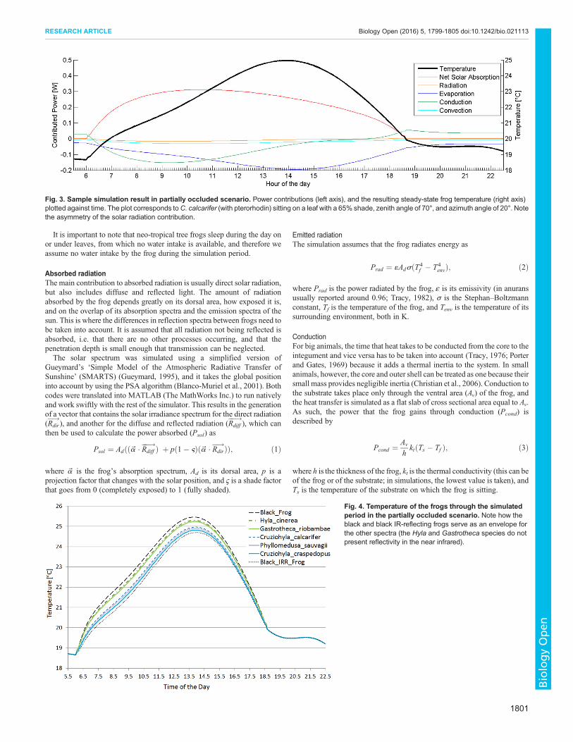
Fig 3 Sample simulation result in partially occluded scenario Power contributions (left axis) and the resulting steady-state frog temperature (right axis)plotted against time The plot corresponds toC calcarifer (with pterorhodin) sitting on a leaf with a 65 shade zenith angle of 70deg and azimuth angle of 20deg Notethe asymmetry of the solar radiation contribution

Fig 4 Temperature of the frogs through the simulatedperiod in the partially occluded scenario Note how theblack and black IR-reflecting frogs serve as an envelope forthe other spectra (the Hyla and Gastrotheca species do notpresent reflectivity in the near infrared)

1801

RESEARCH ARTICLE Biology Open (2016) 5 1799-1805 doi101242bio021113

BiologyOpen

ConvectionThe heat that the air surrounding the frog takes away is simulated as

Pconv frac14 hcAdethTf TaTHORN eth4THORNwhere Pconv is the power the frog loses through convection hc is a heattransfer coefficient which has been approximated in the past as a function ofwind speed (Porter and Gates 1969 Mitchell 1976) and Ta is thetemperature of the air surrounding the frog

Evaporative water loss (EWL)Water evaporation through the skin is one of the main elements controllingthe cooling process in most anurans (Bartelt and Peterson 2005) Tree frogsusually sit in a water-conserving posture that creates a water-tight sealaround their ventral area limiting the evaporation surface to their dorsalarea The rate at which water is being evaporated will vary greatly betweenspecies due to skin properties (Tracy et al 2010) and it will also changedepending on the water vapour pressure difference between the frog and theair around it and of course also on wind velocities (Tracy and Christian2005) The evaporation rate for most anurans can be simulated using afree water surface (Tracy 1976) and as such the frogrsquos water vapourdensity (ρs) can be directly imputed from the saturation value which can befound in tables (httpwwwengineeringtoolboxcomwater-vapor-saturation-pressure-air-d_689html) The surrounding air will have a water vapourdensity (ρa) equal to the product of the saturation value and the relativehumidity (RH)The power exchanged through EWL is given by

PEWL frac14 LhDAdethrs raTHORN eth5THORNwhere L is the latent heat of water (L=2260 kJkg) and hD is the masstransfer coefficient which accounts for the variation in evaporation rates dueto species shape and wind speed

The mass transfer coefficient was measured in agar models following theexperimental method described by Tracy (1976) Five differently shapedmodels were measured at five different wind velocities and two orientationsrelative to the wind direction Two of the models were based on Cruziohylacalcarifer frogs of snout-vent lengths of 61 cm and 43 cm two were basedon Cruziohyla craspedopus frogs of 48 cm and 31 cm and the last modelwas a hemisphere of 31 cm diameter

A total of seven parameters were measured mass time dorsal area windspeed temperature of the frog air temperature and relative humidity Foreach experiment the wind tunnel was set at a speed and left to stabilizeThen a model or group of models were introduced to thewind tunnel and setat an angle of either 0deg or 90deg relative to the wind direction Once thetemperature change stabilized the modelrsquos mass and temperature as well asthe airrsquos temperature and relative humidity were monitored at regular

intervals for a set period of time The frog models had to be momentarilyremoved from the wind tunnel to be weighed each time

The experiments took place in the facilities of the School of MechanicalAerospace and Civil Engineering at the University of Manchester where thelsquoArmfield Tunnelrsquo was chosen for its capacity to produce steady low windspeeds (1 ms to 5 ms) needed for this experiment The speed was measuredwith a precision of 01 ms The frog models were weighed using a KernEMB500-1 precision scale with an accuracy of 01 g The surface area of themodels was the same as the moulds printed for them for which accuracysimilar to that of the 3D rendering technique is expected ie an error of25 The temperature of the frog was measured with an 8889 IRthermometer with an accuracy of 05degC The air temperature and relativehumidity were monitored with an HTD-625 hygrometer-thermometer withan accuracy of 05degC and 2 respectively Measurements were taken every5 min for wind speeds around 5 ms every 75 min for velocities around 3and 4 ms and every 10 min for speeds around 1 and 2 ms The orientationof the models was only measured qualitatively

A total of 80 complete measurements were acquired at 146 ms 212 ms282 ms 38 ms and 463 ms All five differently shaped models weretested at a 0deg orientation (with the head pointing towards the wind) At 90deg(perpendicular to the wind) only the models of the twoC calcarifer and thebigger C craspedopus were tested

It is difficult to maintain wind speeds lower than the ms level in windtunnels and therefore low velocity measurements are very difficult toobtain Since in tropical forests wind speeds are usually of the order cmsbeing able to extrapolate values of the mass transfer coefficient is necessary

It is important to note that hD should have a positive and non-zerointercept which represents the water being evaporated from the frog whenthere is no wind Also since with no wind the evaporation rate would notdepend on shape but only on dorsal area the data for all models shouldconverge to a single intercept On the other side as wind velocities increasethe mass transfer coefficients should diverge between different shapes asTracy (1976) suggests

Cussler (2009) proposes a relationship between the mass transfercoefficient and the wind velocity of the form hdsimv12 but when applied toour data negative intercepts were found A linear or a quadratic relationshipresult in positive intercepts but with a very wide spread

To emphasize the low wind speed interpolation and taking into accountthe divergence between different shapes at higher wind velocities anexperimental fit is proposed (see Fig 5) which follows a relationship of theform

hD frac14 Aek vp eth6THORNwhere v is the wind speed in ms and A k and p are experimentallydetermined constants

Avalue of P=039 was found bymaximizing R2 in a fit for all models andthe other two parameters were allowed to change between frog models

Fig 5 Mass transfer coefficient plotted against the windspeed to the power of 039 Dashed lines are fitted curvesfor single models and the thick red line includes all the dataAll fitted lines are of the form described in Eqn 6 Note that theintercept points converge and diverges for different shapes athigher wind speeds

1802

RESEARCH ARTICLE Biology Open (2016) 5 1799-1805 doi101242bio021113

BiologyOpen

It is important to note that neo-tropical tree frogs sleep during the day onor under leaves from which no water intake is available and therefore weassume no water intake by the frog during the simulation period

Absorbed radiationThe main contribution to absorbed radiation is usually direct solar radiationbut also includes diffuse and reflected light The amount of radiationabsorbed by the frog depends greatly on its dorsal area how exposed it isand on the overlap of its absorption spectra and the emission spectra of thesun This is where the differences in reflection spectra between frogs need tobe taken into account It is assumed that all radiation not being reflected isabsorbed ie that there are no other processes occurring and that thepenetration depth is small enough that transmission can be neglected

The solar spectrum was simulated using a simplified version ofGueymardrsquos lsquoSimple Model of the Atmospheric Radiative Transfer ofSunshinersquo (SMARTS) (Gueymard 1995) and it takes the global positioninto account by using the PSA algorithm (Blanco-Muriel et al 2001) Bothcodes were translated into MATLAB (The MathWorks Inc) to run nativelyand work swiftly with the rest of the simulator This results in the generationof a vector that contains the solar irradiance spectrum for the direct radiation(Rdir

) and another for the diffuse and reflected radiation (Rdiff

) which canthen be used to calculate the power absorbed (Psol) as

Psol frac14 Adetheth~a RdiffTHORN thorn peth1 6THORNeth~a Rdir

THORNTHORN eth1THORN

where ~a is the frogrsquos absorption spectrum Ad is its dorsal area p is aprojection factor that changes with the solar position and ς is a shade factorthat goes from 0 (completely exposed) to 1 (fully shaded)

Emitted radiationThe simulation assumes that the frog radiates energy as

Prad frac14 1AdsethT 4f T4

envTHORN eth2THORN

where Prad is the power radiated by the frog ε is its emissivity (in anuransusually reported around 096 Tracy 1982) σ is the StephanndashBoltzmannconstant Tf is the temperature of the frog and Tenv is the temperature of itssurrounding environment both in K

ConductionFor big animals the time that heat takes to be conducted from the core to theintegument and vice versa has to be taken into account (Tracy 1976 Porterand Gates 1969) because it adds a thermal inertia to the system In smallanimals however the core and outer shell can be treated as one because theirsmall mass provides negligible inertia (Christian et al 2006) Conduction tothe substrate takes place only through the ventral area (Av) of the frog andthe heat transfer is simulated as a flat slab of cross sectional area equal to AvAs such the power that the frog gains through conduction (Pcond) isdescribed by

Pcond frac14 Av

hktethTs Tf THORN eth3THORN

where h is the thickness of the frog kt is the thermal conductivity (this can beof the frog or of the substrate in simulations the lowest value is taken) andTs is the temperature of the substrate on which the frog is sitting

Fig 3 Sample simulation result in partially occluded scenario Power contributions (left axis) and the resulting steady-state frog temperature (right axis)plotted against time The plot corresponds toC calcarifer (with pterorhodin) sitting on a leaf with a 65 shade zenith angle of 70deg and azimuth angle of 20deg Notethe asymmetry of the solar radiation contribution

Fig 4 Temperature of the frogs through the simulatedperiod in the partially occluded scenario Note how theblack and black IR-reflecting frogs serve as an envelope forthe other spectra (the Hyla and Gastrotheca species do notpresent reflectivity in the near infrared)

1801

RESEARCH ARTICLE Biology Open (2016) 5 1799-1805 doi101242bio021113

BiologyOpen

ConvectionThe heat that the air surrounding the frog takes away is simulated as

Pconv frac14 hcAdethTf TaTHORN eth4THORNwhere Pconv is the power the frog loses through convection hc is a heattransfer coefficient which has been approximated in the past as a function ofwind speed (Porter and Gates 1969 Mitchell 1976) and Ta is thetemperature of the air surrounding the frog

Evaporative water loss (EWL)Water evaporation through the skin is one of the main elements controllingthe cooling process in most anurans (Bartelt and Peterson 2005) Tree frogsusually sit in a water-conserving posture that creates a water-tight sealaround their ventral area limiting the evaporation surface to their dorsalarea The rate at which water is being evaporated will vary greatly betweenspecies due to skin properties (Tracy et al 2010) and it will also changedepending on the water vapour pressure difference between the frog and theair around it and of course also on wind velocities (Tracy and Christian2005) The evaporation rate for most anurans can be simulated using afree water surface (Tracy 1976) and as such the frogrsquos water vapourdensity (ρs) can be directly imputed from the saturation value which can befound in tables (httpwwwengineeringtoolboxcomwater-vapor-saturation-pressure-air-d_689html) The surrounding air will have a water vapourdensity (ρa) equal to the product of the saturation value and the relativehumidity (RH)The power exchanged through EWL is given by

PEWL frac14 LhDAdethrs raTHORN eth5THORNwhere L is the latent heat of water (L=2260 kJkg) and hD is the masstransfer coefficient which accounts for the variation in evaporation rates dueto species shape and wind speed

The mass transfer coefficient was measured in agar models following theexperimental method described by Tracy (1976) Five differently shapedmodels were measured at five different wind velocities and two orientationsrelative to the wind direction Two of the models were based on Cruziohylacalcarifer frogs of snout-vent lengths of 61 cm and 43 cm two were basedon Cruziohyla craspedopus frogs of 48 cm and 31 cm and the last modelwas a hemisphere of 31 cm diameter

A total of seven parameters were measured mass time dorsal area windspeed temperature of the frog air temperature and relative humidity Foreach experiment the wind tunnel was set at a speed and left to stabilizeThen a model or group of models were introduced to thewind tunnel and setat an angle of either 0deg or 90deg relative to the wind direction Once thetemperature change stabilized the modelrsquos mass and temperature as well asthe airrsquos temperature and relative humidity were monitored at regular

intervals for a set period of time The frog models had to be momentarilyremoved from the wind tunnel to be weighed each time

The experiments took place in the facilities of the School of MechanicalAerospace and Civil Engineering at the University of Manchester where thelsquoArmfield Tunnelrsquo was chosen for its capacity to produce steady low windspeeds (1 ms to 5 ms) needed for this experiment The speed was measuredwith a precision of 01 ms The frog models were weighed using a KernEMB500-1 precision scale with an accuracy of 01 g The surface area of themodels was the same as the moulds printed for them for which accuracysimilar to that of the 3D rendering technique is expected ie an error of25 The temperature of the frog was measured with an 8889 IRthermometer with an accuracy of 05degC The air temperature and relativehumidity were monitored with an HTD-625 hygrometer-thermometer withan accuracy of 05degC and 2 respectively Measurements were taken every5 min for wind speeds around 5 ms every 75 min for velocities around 3and 4 ms and every 10 min for speeds around 1 and 2 ms The orientationof the models was only measured qualitatively

A total of 80 complete measurements were acquired at 146 ms 212 ms282 ms 38 ms and 463 ms All five differently shaped models weretested at a 0deg orientation (with the head pointing towards the wind) At 90deg(perpendicular to the wind) only the models of the twoC calcarifer and thebigger C craspedopus were tested

It is difficult to maintain wind speeds lower than the ms level in windtunnels and therefore low velocity measurements are very difficult toobtain Since in tropical forests wind speeds are usually of the order cmsbeing able to extrapolate values of the mass transfer coefficient is necessary

It is important to note that hD should have a positive and non-zerointercept which represents the water being evaporated from the frog whenthere is no wind Also since with no wind the evaporation rate would notdepend on shape but only on dorsal area the data for all models shouldconverge to a single intercept On the other side as wind velocities increasethe mass transfer coefficients should diverge between different shapes asTracy (1976) suggests

Cussler (2009) proposes a relationship between the mass transfercoefficient and the wind velocity of the form hdsimv12 but when applied toour data negative intercepts were found A linear or a quadratic relationshipresult in positive intercepts but with a very wide spread

To emphasize the low wind speed interpolation and taking into accountthe divergence between different shapes at higher wind velocities anexperimental fit is proposed (see Fig 5) which follows a relationship of theform

hD frac14 Aek vp eth6THORNwhere v is the wind speed in ms and A k and p are experimentallydetermined constants

Avalue of P=039 was found bymaximizing R2 in a fit for all models andthe other two parameters were allowed to change between frog models

Fig 5 Mass transfer coefficient plotted against the windspeed to the power of 039 Dashed lines are fitted curvesfor single models and the thick red line includes all the dataAll fitted lines are of the form described in Eqn 6 Note that theintercept points converge and diverges for different shapes athigher wind speeds

1802

RESEARCH ARTICLE Biology Open (2016) 5 1799-1805 doi101242bio021113

BiologyOpen

ConvectionThe heat that the air surrounding the frog takes away is simulated as

Pconv frac14 hcAdethTf TaTHORN eth4THORNwhere Pconv is the power the frog loses through convection hc is a heattransfer coefficient which has been approximated in the past as a function ofwind speed (Porter and Gates 1969 Mitchell 1976) and Ta is thetemperature of the air surrounding the frog

Evaporative water loss (EWL)Water evaporation through the skin is one of the main elements controllingthe cooling process in most anurans (Bartelt and Peterson 2005) Tree frogsusually sit in a water-conserving posture that creates a water-tight sealaround their ventral area limiting the evaporation surface to their dorsalarea The rate at which water is being evaporated will vary greatly betweenspecies due to skin properties (Tracy et al 2010) and it will also changedepending on the water vapour pressure difference between the frog and theair around it and of course also on wind velocities (Tracy and Christian2005) The evaporation rate for most anurans can be simulated using afree water surface (Tracy 1976) and as such the frogrsquos water vapourdensity (ρs) can be directly imputed from the saturation value which can befound in tables (httpwwwengineeringtoolboxcomwater-vapor-saturation-pressure-air-d_689html) The surrounding air will have a water vapourdensity (ρa) equal to the product of the saturation value and the relativehumidity (RH)The power exchanged through EWL is given by

PEWL frac14 LhDAdethrs raTHORN eth5THORNwhere L is the latent heat of water (L=2260 kJkg) and hD is the masstransfer coefficient which accounts for the variation in evaporation rates dueto species shape and wind speed

The mass transfer coefficient was measured in agar models following theexperimental method described by Tracy (1976) Five differently shapedmodels were measured at five different wind velocities and two orientationsrelative to the wind direction Two of the models were based on Cruziohylacalcarifer frogs of snout-vent lengths of 61 cm and 43 cm two were basedon Cruziohyla craspedopus frogs of 48 cm and 31 cm and the last modelwas a hemisphere of 31 cm diameter

A total of seven parameters were measured mass time dorsal area windspeed temperature of the frog air temperature and relative humidity Foreach experiment the wind tunnel was set at a speed and left to stabilizeThen a model or group of models were introduced to thewind tunnel and setat an angle of either 0deg or 90deg relative to the wind direction Once thetemperature change stabilized the modelrsquos mass and temperature as well asthe airrsquos temperature and relative humidity were monitored at regular

intervals for a set period of time The frog models had to be momentarilyremoved from the wind tunnel to be weighed each time

The experiments took place in the facilities of the School of MechanicalAerospace and Civil Engineering at the University of Manchester where thelsquoArmfield Tunnelrsquo was chosen for its capacity to produce steady low windspeeds (1 ms to 5 ms) needed for this experiment The speed was measuredwith a precision of 01 ms The frog models were weighed using a KernEMB500-1 precision scale with an accuracy of 01 g The surface area of themodels was the same as the moulds printed for them for which accuracysimilar to that of the 3D rendering technique is expected ie an error of25 The temperature of the frog was measured with an 8889 IRthermometer with an accuracy of 05degC The air temperature and relativehumidity were monitored with an HTD-625 hygrometer-thermometer withan accuracy of 05degC and 2 respectively Measurements were taken every5 min for wind speeds around 5 ms every 75 min for velocities around 3and 4 ms and every 10 min for speeds around 1 and 2 ms The orientationof the models was only measured qualitatively

A total of 80 complete measurements were acquired at 146 ms 212 ms282 ms 38 ms and 463 ms All five differently shaped models weretested at a 0deg orientation (with the head pointing towards the wind) At 90deg(perpendicular to the wind) only the models of the twoC calcarifer and thebigger C craspedopus were tested

It is difficult to maintain wind speeds lower than the ms level in windtunnels and therefore low velocity measurements are very difficult toobtain Since in tropical forests wind speeds are usually of the order cmsbeing able to extrapolate values of the mass transfer coefficient is necessary

It is important to note that hD should have a positive and non-zerointercept which represents the water being evaporated from the frog whenthere is no wind Also since with no wind the evaporation rate would notdepend on shape but only on dorsal area the data for all models shouldconverge to a single intercept On the other side as wind velocities increasethe mass transfer coefficients should diverge between different shapes asTracy (1976) suggests

Cussler (2009) proposes a relationship between the mass transfercoefficient and the wind velocity of the form hdsimv12 but when applied toour data negative intercepts were found A linear or a quadratic relationshipresult in positive intercepts but with a very wide spread

To emphasize the low wind speed interpolation and taking into accountthe divergence between different shapes at higher wind velocities anexperimental fit is proposed (see Fig 5) which follows a relationship of theform

hD frac14 Aek vp eth6THORNwhere v is the wind speed in ms and A k and p are experimentallydetermined constants

Avalue of P=039 was found bymaximizing R2 in a fit for all models andthe other two parameters were allowed to change between frog models

Fig 5 Mass transfer coefficient plotted against the windspeed to the power of 039 Dashed lines are fitted curvesfor single models and the thick red line includes all the dataAll fitted lines are of the form described in Eqn 6 Note that theintercept points converge and diverges for different shapes athigher wind speeds

1802

RESEARCH ARTICLE Biology Open (2016) 5 1799-1805 doi101242bio021113

BiologyOpen

reaching an average of A=00041 ms and k=140 (sm)p It is imperative tostress however that this relationship is only proposed to fit the data with anemphasis on the intercept point which is essential in the simulation butthere is no theoretical basis for it

Surface areasAll the thermoregulatory processes are affected by the surface area of thefrogs whether it is ventral area or dorsal area During the simulation theseareas can be approximated in different ways One method is to model thefrog as a hemisphere of a given radius estimated from the mass of the frogor inferred from the snout-vent length Alternatively actual surface areasrelated to a specific frog species can be used if these are known

To address this issue a non-invasive technique to measure the surfacearea of the frogs was developed by rendering a 3D model of the specimenfrom a series of photographs taken at different angles The technique wastested in the two different species of the Criziohyla genus and was found tobe accurate to 12 in snout-vent measurements and 25 in surface andvolume measurements

In collaboration with the Vivarium at the Manchester Museum a total of23 C craspeopus and 20 C calcarifer of different sizes and at differentstages of development were photographed and their 3D models rendered inorder to measure their surface areas and volume

TheC craspedopus specimens ranged from 31 cm snout-vent and 2 g to58 cm snout-vent and 15 g This covers sizes from frogs a few weeks afterhatching to nearly fully grown adults The C calcarifer specimens rangedfrom 33 cm snout-vent and 3 g to 64 cm snout-vent and 23 g which also

covers from very young froglets up to fully developedmale adults which areusually a bit smaller than adult females

The specimens were placed on a turn table and slowly rotated whilephotographs were taken at no more than 15deg intervals and from two differentheights (sim20 and 40 cm) Animal handling was performed by the trainedstaff of the Vivarium at TheManchester Museum conform to all regulationsand animal welfare laws

The 3D models were rendered using Smart3DCapture 311 (httpscommunityacute3dcomsmart3dcapture-free-edition) which accepts aseries of photographs from different angles as input reconstructs thephotographed object and outputs a mesh The mesh was further cleanedand corrected using Blender 273 (httpwwwblenderorg) The finalizedmesh is a series of triangles with vertices spatially localized and so it iseasy to calculate areas of very complex shapes The surface and volumeof the mesh was computed using NeuroMorph toolkit (Jorstad et al2014)

The accuracy of the technique was evaluated either by comparing therendered size of objects with regular shapes known density or with printed3D models in which case the mesh size of the pre-print and the post-printversion were compared In all cases the absolute average error was under12 for linear measurements (ie snout-vent) and 25 for surface andvolume measurements See Herreriacuteas-Azcueacute (2015) for further detail

Mass inferenceInterpolation of surface area from mass has already been reported in theliterature (Tracy 1976 Hutchison et al 1968 McClanahan and

Fig 6 Surface areas plotted against the mass of the frog Fittedlines follow the power function described in Eqn 7 Note how closelyoverlapped the fitted lines are which suggests very similar surfacearea in both species

Fig 7 Surface areas plotted against the snout-vent lengthsquared Fitted lines follow the function described in Eqn 8 Notehow the lines are clearly separated which suggests clearly distinctsurface area between species

1803

RESEARCH ARTICLE Biology Open (2016) 5 1799-1805 doi101242bio021113

BiologyOpen

Baldwin 1969) often by fitting the surface area to a power function ofthe mass (w)

Ad frac14 aethwbTHORNAv frac14 cethwdTHORN eth7THORNThe constants a b c and d are determined experimentally by fitting a

curve to the experimental data Fig 6 shows the acquired measurements ofthe two species with masses ranging from 2 g to 23 g and the power fitcorresponding to each of them For C calcarifer the coefficients werefound to be a=480 b=065 c=308 and d=066 For C craspedopus thecoefficients were found to be a=504 b=063 c=292 and d=070

Snout-vent inferenceIt is natural to expect a relationship between the snout-vent length of a frog ameasure of its size and its surface area Furthermore it is a measurementthat is usually gathered in any observation of a species so it is a veryconvenient datum from which to start

As can be seen in Fig 7 there is a clear link between the snout-vent lengthsquared and the surface areas for which the interpolation proposed is simply

Ad frac14 SdethLsvTHORN2Av frac14 SvethLsvTHORN2 eth8THORNwhere Lsv is the snout-vent length and the constants Sd and Sv aredetermined with the linear fit The coefficients found for C calcarifer wereSd=081 and Sv=053 whereas for C craspedopus they were found to beSd=085 and Sv=058

Simulation scenariosThe simulator receives inputs that will determine the heat transfermechanisms already described and finds the equilibrium temperature ofthe frog at set intervals for the whole simulation period Since the airtemperature wind speed and humidity are very likely to change in a longsimulation an ambient profile can be introduced to yield more accurateresults The ambient profile used for the simulations reported here is shownin Fig 8 and was obtained from interpolated meteorological reports fromAmazonian forests (Lowman and Rinker 2004) combined with the wind

speed differences between substrate level and at the canopies described in(Baynton et al 1965)

Two different scenarios were simulated One of them proposes the mostextreme circumstances for a frog where it is fully exposed to the sun andsitting flat on the ground The other one is perhaps a more realistic scenarioand it represents a partially occluded frog The shade factor was setto ς=065 it was perched on a leaf at an angle of 70deg from the vertical leaningto the NNE All other inputs were the same in both scenarios which meansthat the only difference between the frogs simulated is their reflectionspectra

The sample spectra shown in Fig 9 were measured from specimens beingheld at TheManchesterMuseumrsquosVivarium using anOceanOptics USB4000-VIS-NIR spectrometer Due to the lack of accuracy of the spectrometer outsideof the 450-950 nm range the measurements were truncated at 450 nm and950 nm and an exponential fall off (eminus5) was added at the edges Most of theradiated energy of the sun that is available for absorption by the frog falls withinthis range and spectra of different species has been found to be very similar outof it (Emerson et al 1990) for which changes in temperature between speciesdue to absorption out of that range would be even less relevant

The depicted spectra are the result of the average of five measurementssmoothed with a 10 wide boxcar method Water absorption bands are notvisible due to the truncation and exponential fall-off

Three species with the characteristic IR reflectance peak (C calcariferC craspedopus and Phyllomedusa sauvagii) and two without it(Gastrotheca riobambae and Hyla cinerea) were considered as well as acompletely absorbent (black) spectrum (α=1) and a black IRR-reflectivespectrum (α=0 if 700 nmleλle1500 mm and α=1 in any other case) used asreferences

The program internally converts these reflection spectra (~Y) to absorptionspectra (~a) using

~a frac14 1 ~Y eth9THORN

The frogsrsquo size global position and thermal properties were fixed for allspectra

Fig 8 Ambient profile used in the simulations Ambienttemperature wind speed and relative humidity throughout thesimulated day The relative humidity was divided by a factor of10 so that it could be shown next to the wind speed

Fig 9 Examples of reflectionspectra of frogs Note how some ofthe used spectra show the near infra-red reflection peak at sim700 nm andsome do not The dotted and dashedlines are extreme reference spectrabuilt for a completely black frog and ablack infrared reflective frog Anexponential fall of was forced after1000 nm

1804

RESEARCH ARTICLE Biology Open (2016) 5 1799-1805 doi101242bio021113

BiologyOpen

The significance of the temperature differences in the frogs was evaluatedalso through its effect on water conservation as previously suggested inTracy et al (2010) As the simulation progresses the mass of the frogdecreases due to EWL Since they can hold up to 20 of their weight in theirbladder (Shoemaker et al 1989) a lsquorehydration boundaryrsquowas set at 80 oftheir weight and the time elapsed before this limit is reached is quoted Afterthat the frog would necessarily need to rehydrate which implies movingand being exposed while water is being absorbed We refer to this as arehydration event

AcknowledgementsThe authors would like to thank Andrew Gray Adam Bland and Matthew OrsquoDonnell(Manchester Museumrsquos Vivarium) for their support in providing and handling the livefrog specimens used in this study

Competing interestsThe authors declare no competing or financial interests

Data availabilityAll measurements simulation data and the simulator code can be obtained byrequest to the corresponding author or at the University of Manchester datarepository under ESCHOLARPID uk-ac-man-scw305404 (httpswwwescholarmanchesteracukuk-ac-man-scw305404)

Author contributionsFHA designed and performed researched analysed data and wrotemanuscript C B contributed with frog spectra measurements and data analysisMD designed research and wrote manuscript

FundingThis work was partially funded by the Mexican National Council for Science andTechnology (Consejo Nacional de Ciencia y Tecnologıa CONACyT) [grantnumbers 327566 and 381923] in partnership with the University of Manchester

ReferencesBartelt P E and Peterson C R (2005) Physically modeling operativetemperatures and evaporation rates in amphibians J Therm Biol 30 93-102

Baynton H W Biggs W G Hamilton H L Jr Sherr P E and Worth J B(1965) Wind structure in and above a tropical forest J Appl Meteorol 4 670-675

Blanco-Muriel M Alarcon-Padilla D C Lopez-Moratalla T and Lara-CoiraM (2001) Computing the solar vector Sol Energy 70 431-441

Christian K A Tracy C R and Tracy C R (2006) Evaluating thermoregulationin reptiles an appropriate null model Am Nat 168 421-430

Cussler E L (2009)Diffusion Mass Transfer in Fluid Systems 3rd edn NewYorkCambridge University Press

Emerson S B Cooper T A and Ehleringer J R (1990) Convergence inreflectance spectra among treefrogs Funct Ecol 4 47-51

Gueymard C (1995) SMARTS2 A simple Model of the Atmospheric RadiativeTransfer of Sunshine Algorithms and Performance Assessment Florida FloridaSolar Energy CenterUniversity of Central Florida

Herrerıas-Azcue F (2015) Thermoregulation in Neo-Tropical Tree Frogs MPhilthesis University of Manchester Manchester UK

Hutchison V H Whitford W G and Kohl M (1968) Relation of body size andsurface area to gas exchange in anurans Physiol Zool 41 65-85

Jorstad A Nigro B Cali C Wawrzyniak M Fua P and Knott G (2014)NeuroMorph a toolset for the morphometric analysis and visualisation of 3Dmodels derived from electron microscopy image stacks Neuroinformatics 1383-92

Lowman M and Rinker H B (2004) Forest Canopies 2nd edn ElsevierAcademic Press

McClanahan L J and Baldwin R (1969) Rate of water uptake through theintegument of the desert toad Bufo punctatus Comp Biochem Physiol 28381-389

Mitchell J W (1976) Heat transfer from spheres and other animal forms BiophysJ 16 561-569

Porter W P and Gates D M (1969) Thermodynamic equilibria of animals withenvironment Ecol Monogr 39 227-244

Schwalm P A Starrett P H and McDiarmid R W (1977) Infrared reflectancein leaf-sitting neotropical frogs Science 196 3-4

Shoemaker V H Baker M A and Loveridge J P (1989) Effect of waterbalance on thermoregulation in waterproof frogs (Chiromantis andPhyllomedusa) Physiol Zool 62 133-146

Tracy C R (1976) A model of the dynamic exchanges of water and energybetween a terrestrial amphibian and its environment Ecol Monogr 46293-326

Tracy C R (1982) Biophysical Modeling in Reptilian Physiology and Ecology InBiology of the Reptilia (ed C Gans and F Harvey Pough) 2nd edn pp 275-321Academic Press

Tracy C R and Christian K A (2005) Preferred temperature correlates withevaporative water loss in hylid frogs from northern Australia Physiol BiochemZool 78 839-846

Tracy C R Christian K A and Tracy C R (2010) Not just small wet and coldeffects of body size and skin resistance on thermoregulation and arboreality offrogs Ecology 91 1477-1484

1805

RESEARCH ARTICLE Biology Open (2016) 5 1799-1805 doi101242bio021113

BiologyOpen

The significance of the temperature differences in the frogs was evaluatedalso through its effect on water conservation as previously suggested inTracy et al (2010) As the simulation progresses the mass of the frogdecreases due to EWL Since they can hold up to 20 of their weight in theirbladder (Shoemaker et al 1989) a lsquorehydration boundaryrsquowas set at 80 oftheir weight and the time elapsed before this limit is reached is quoted Afterthat the frog would necessarily need to rehydrate which implies movingand being exposed while water is being absorbed We refer to this as arehydration event

AcknowledgementsThe authors would like to thank Andrew Gray Adam Bland and Matthew OrsquoDonnell(Manchester Museumrsquos Vivarium) for their support in providing and handling the livefrog specimens used in this study

Competing interestsThe authors declare no competing or financial interests

Data availabilityAll measurements simulation data and the simulator code can be obtained byrequest to the corresponding author or at the University of Manchester datarepository under ESCHOLARPID uk-ac-man-scw305404 (httpswwwescholarmanchesteracukuk-ac-man-scw305404)

Author contributionsFHA designed and performed researched analysed data and wrotemanuscript C B contributed with frog spectra measurements and data analysisMD designed research and wrote manuscript

FundingThis work was partially funded by the Mexican National Council for Science andTechnology (Consejo Nacional de Ciencia y Tecnologıa CONACyT) [grantnumbers 327566 and 381923] in partnership with the University of Manchester

ReferencesBartelt P E and Peterson C R (2005) Physically modeling operativetemperatures and evaporation rates in amphibians J Therm Biol 30 93-102

Baynton H W Biggs W G Hamilton H L Jr Sherr P E and Worth J B(1965) Wind structure in and above a tropical forest J Appl Meteorol 4 670-675

Blanco-Muriel M Alarcon-Padilla D C Lopez-Moratalla T and Lara-CoiraM (2001) Computing the solar vector Sol Energy 70 431-441

Christian K A Tracy C R and Tracy C R (2006) Evaluating thermoregulationin reptiles an appropriate null model Am Nat 168 421-430

Cussler E L (2009)Diffusion Mass Transfer in Fluid Systems 3rd edn NewYorkCambridge University Press

Emerson S B Cooper T A and Ehleringer J R (1990) Convergence inreflectance spectra among treefrogs Funct Ecol 4 47-51

Gueymard C (1995) SMARTS2 A simple Model of the Atmospheric RadiativeTransfer of Sunshine Algorithms and Performance Assessment Florida FloridaSolar Energy CenterUniversity of Central Florida

Herrerıas-Azcue F (2015) Thermoregulation in Neo-Tropical Tree Frogs MPhilthesis University of Manchester Manchester UK

Hutchison V H Whitford W G and Kohl M (1968) Relation of body size andsurface area to gas exchange in anurans Physiol Zool 41 65-85

Jorstad A Nigro B Cali C Wawrzyniak M Fua P and Knott G (2014)NeuroMorph a toolset for the morphometric analysis and visualisation of 3Dmodels derived from electron microscopy image stacks Neuroinformatics 1383-92

Lowman M and Rinker H B (2004) Forest Canopies 2nd edn ElsevierAcademic Press

McClanahan L J and Baldwin R (1969) Rate of water uptake through theintegument of the desert toad Bufo punctatus Comp Biochem Physiol 28381-389

Mitchell J W (1976) Heat transfer from spheres and other animal forms BiophysJ 16 561-569

Porter W P and Gates D M (1969) Thermodynamic equilibria of animals withenvironment Ecol Monogr 39 227-244

Schwalm P A Starrett P H and McDiarmid R W (1977) Infrared reflectancein leaf-sitting neotropical frogs Science 196 3-4

Shoemaker V H Baker M A and Loveridge J P (1989) Effect of waterbalance on thermoregulation in waterproof frogs (Chiromantis andPhyllomedusa) Physiol Zool 62 133-146

Tracy C R (1976) A model of the dynamic exchanges of water and energybetween a terrestrial amphibian and its environment Ecol Monogr 46293-326

Tracy C R (1982) Biophysical Modeling in Reptilian Physiology and Ecology InBiology of the Reptilia (ed C Gans and F Harvey Pough) 2nd edn pp 275-321Academic Press

Tracy C R and Christian K A (2005) Preferred temperature correlates withevaporative water loss in hylid frogs from northern Australia Physiol BiochemZool 78 839-846

Tracy C R Christian K A and Tracy C R (2010) Not just small wet and coldeffects of body size and skin resistance on thermoregulation and arboreality offrogs Ecology 91 1477-1484

1805

RESEARCH ARTICLE Biology Open (2016) 5 1799-1805 doi101242bio021113

BiologyOpen
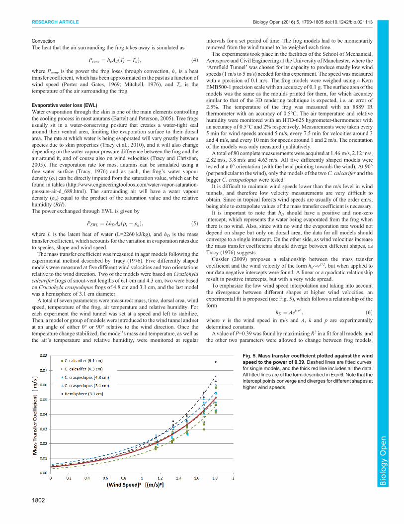