Teletraffic & Queueing Theory Telecommunications Networks1 ELE 511 – TELECOMMUNICATIONS NETWORKS...
33
Teletraffic & Qu eueing Theory Telecommunications Networ ks 1 ELE 511 – TELECOMMUNICATIONS NETWORKS Lecturer: Dr. Thomas Afullo, Department of Electrical Engineering, University of Botswana, Gaborone, Botswana. Tel: 267-3554342; E-mail: [email protected]
-
Upload
naomi-dean -
Category
Documents
-
view
240 -
download
1
Transcript of Teletraffic & Queueing Theory Telecommunications Networks1 ELE 511 – TELECOMMUNICATIONS NETWORKS...
Teletraffic & Queueing Theory
Telecommunications Networks 1
ELE 511 – TELECOMMUNICATIONS NETWORKS
Lecturer: Dr. Thomas Afullo,
Department of Electrical Engineering,
University of Botswana,
Gaborone, Botswana.
Tel: 267-3554342; E-mail: [email protected]
Teletraffic & Queueing Theory
Telecommunications Networks 2
ELE 511 – TELECOMMUNICATIONS NETWORKS
• References:
• 1. R.L. Freeman: Telecommunications Transmission Handbook, Wiley, ISBN 0-471-51816-6.
• 2. J.E. Flood: Telecommunications Switching, Traffic, and Networks, Prentice-Hall, ISBN 0-13-033309-3.
• 3. L. Kleinrock: Queuing Systems Volume 1, Wiley.
Teletraffic & Queueing Theory
Telecommunications Networks 3
TELETRAFFIC & QUEUEING THEORY• INTRODUCTION• Queues and queuing systems have been the subject of considerable research
since the appearance of the first telephone systems.• The widespread use of computers in communication systems has introduced
new results on queuing networks in studies of large communication networks.• The methods of queuing networks have therefore been a basic component of
telecommunication networks. Most problems involving modeling computer systems or data transmission networks deal with systems having multiple resources (central processing units, channels, memories, communication circuits, etc) to be taken into account. This complex structure leads to the study of queuing networks rather than simple queues with a single server.
• We study queues in order to be able to predict the effect of changes on the system before we can actually implement changes on various parameters, like a) pattern of arrivals, b) mean length of service, and c) the number of servers.
• Then we determine how these changes will affect: a) The average time customers have to wait for service; b) The average number of waiting customers; c) The proportion of time the facility is used.
Teletraffic & Queueing Theory
Telecommunications Networks 4
TELETRAFFIC & QUEUEING THEORY• INTRODUCTION
• There are three basic elements in a queuing system:
• 1. The arrivals:
• To describe the arrivals to a queuing system, we need to consider the statistical patterns of the arrivals.
• Possibilities include regular arrivals or irregular arrivals, with the inter-arrival times having some specified distribution. In such cases, we can define the arrival rate, or the average number of arrivals per second.
• 2. The service mechanism:
• To describe this, we need to know the number of servers and the average duration of service time.
• 3. The service discipline:
• Generally, the discipline is first-in-first-out (FIFO), but others are possible in which certain customers get priority. An obvious example is accident victims who are very seriously injured – they would jump the queue to get fast treatment.

Teletraffic & Queueing Theory
Telecommunications Networks 5
TELETRAFFIC & QUEUEING THEORY
• INTRODUCTORY PROBABILITY THEORY
• If A and B are two arbitrary events, then from the set identity:
• Then, probability of A or B is given by:
• Also we get:
• Then, from the above two equations, we have:
• If A and B are independent events, and for n mutually independent events, we have:
)(AcomplementA
BAABA
BAPAPBAP
BAPABPBPBAABB
ABPBPAPBAP
nn APAPAPAAAP
BPAPABP
...,...,, 2121
Teletraffic & Queueing Theory
Telecommunications Networks 6
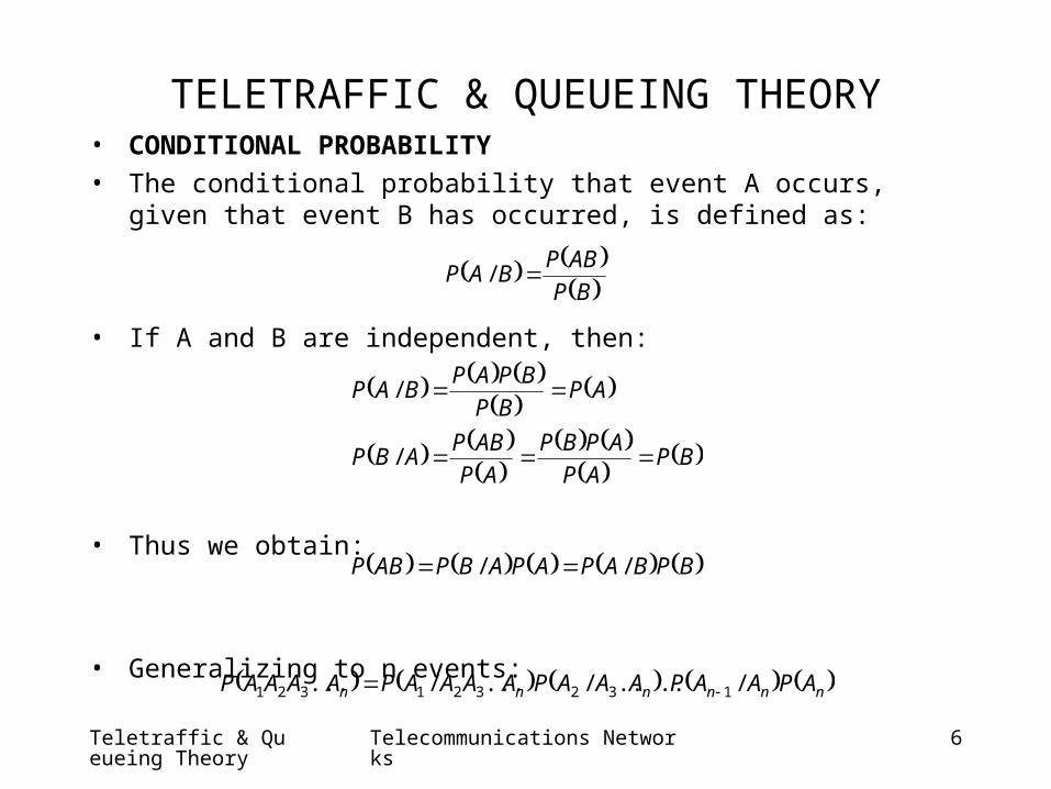
TELETRAFFIC & QUEUEING THEORY• CONDITIONAL PROBABILITY
• The conditional probability that event A occurs, given that event B has occurred, is defined as:
• If A and B are independent, then:
• Thus we obtain:
• Generalizing to n events:
BP
ABPBAP /
BPAP
APBP
AP
ABPABP
APBP
BPAPBAP
/
/
BPBAPAPABPABP //
nnnnnn APAAPAAAPAAAAPAAAAP /..../.../... 132321321
Teletraffic & Queueing Theory
Telecommunications Networks 7
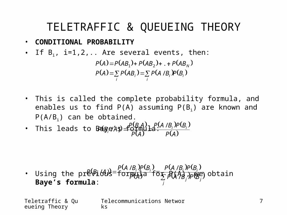
TELETRAFFIC & QUEUEING THEORY• CONDITIONAL PROBABILITY
• If Bi, i=1,2,.. Are several events, then:
• This is called the complete probability formula, and enables us to find P(A) assuming P(Bi) are known and P(A/Bi) can be obtained.
• This leads to Baye’s formula:
• Using the previous formula for P(A), we obtain Baye’s formula:
i
ii
ii
N
BPBAPABPAP
ABPABPABPAP
/
..21
AP
BPBAP
AP
ABPABP iii
i
/)/
jjj
iiiii BPBAP
BPBAP
AP
BPBAPABP
/
//)/
Teletraffic & Queueing Theory
Telecommunications Networks 8
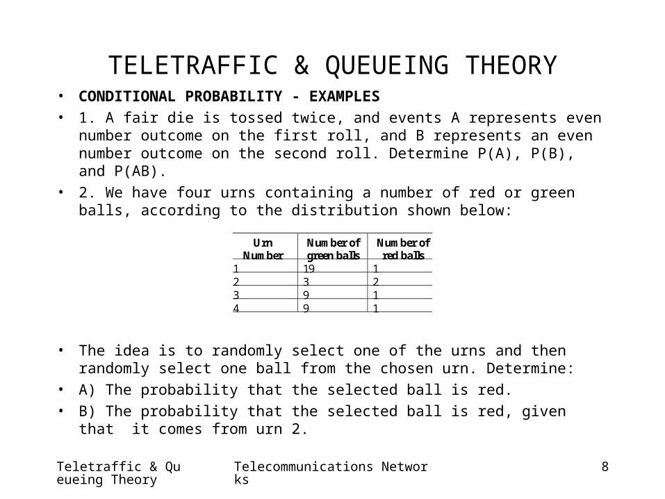
TELETRAFFIC & QUEUEING THEORY• CONDITIONAL PROBABILITY - EXAMPLES
• 1. A fair die is tossed twice, and events A represents even number outcome on the first roll, and B represents an even number outcome on the second roll. Determine P(A), P(B), and P(AB).
• 2. We have four urns containing a number of red or green balls, according to the distribution shown below:
• The idea is to randomly select one of the urns and then randomly select one ball from the chosen urn. Determine:
• A) The probability that the selected ball is red.
• B) The probability that the selected ball is red, given that it comes from urn 2.
Urn Number
Number of green balls
Number of red balls
1 19 1 2 3 2 3 9 1 4 9 1

Teletraffic & Queueing Theory
Telecommunications Networks 9
TELETRAFFIC & QUEUEING THEORY• RANDOM VARIABLES
• It is often required to consider the behavior of functions defined on a sample space and whose values are real numbers.
• These functions are called random variables, where the term random refers to the fact that the value of the function is known only after the experiment has been performed.
• The probability that a random variable, X, takes a value which does not exceed a given number, x, is called the cumulative distribution function (CDF) of X, denoted by F(x). Thus:
•
• The CDF of any random variable has the following properties:
xxXPxF ,
1,
1,0
,
lim
ixFxF
FF
yxforyFxF
ii

Teletraffic & Queueing Theory
Telecommunications Networks 10
TELETRAFFIC & QUEUEING THEORY• RANDOM VARIABLES
• If a and b are two real numbers such that a<b, then the probability that X takes on a value in the interval [a,b] is given by:
• If a=b, then:
• For a continuous random variable X, F(x) is a continuous function of x; we define the probability density function, f(x) as:
• According to the definition of a derivative,
aFbFbxaP
0
0
aFbFbaaP
aFbFba
dx
xdFxf
)()(
x
xxXxP
x
xFxxFxf
xx
limlim
00)(

Teletraffic & Queueing Theory
Telecommunications Networks 11
TELETRAFFIC & QUEUEING THEORY• RANDOM VARIABLES
• Then, when x is small, f(x)x is the probability that the random variable, X, takes a value in the interval [x, x].
• Thus, given a probability density function, f(x), the corresponding cumulative distribution function F(x), is given by:
• In order to ensure that F()=1, we have:
• To find the probability that X falls in the interval [a,b], we have:
x
duufxF )(
1)( duufF
b
a
dxxfbxaP )(
Teletraffic & Queueing Theory
Telecommunications Networks 12
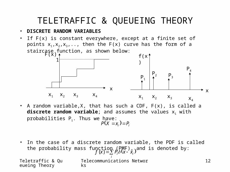
TELETRAFFIC & QUEUEING THEORY• DISCRETE RANDOM VARIABLES
• If F(x) is constant everywhere, except at a finite set of points x1,x2,x3,.., then the F(x) curve has the form of a staircase function, as shown below:
• A random variable,X, that has such a CDF, F(x), is called a discrete random variable; and assumes the values xi with probabilities Pi. Thus we have:
• In the case of a discrete random variable, the PDF is called the probability mass function (PMF), and is denoted by:
x
F(x)
x1 x2 x3 x4
1
x1 x2 x3 x4
x
f(x)
P1
P2 P3
P4
ii PxXP
i
ii xxPxf )(

Teletraffic & Queueing Theory
Telecommunications Networks 13
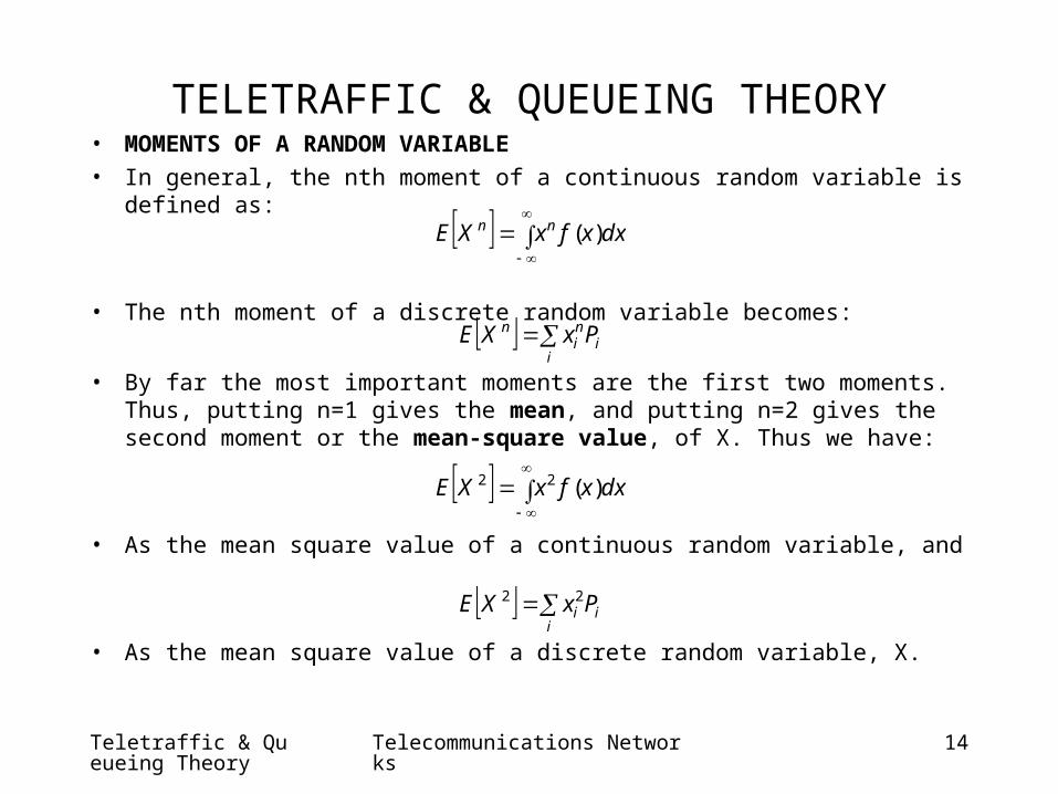
TELETRAFFIC & QUEUEING THEORY• MOMENTS OF A RANDOM VARIABLE
• Although a random variable is characterized completely by either its CDF or PDF/PMF, such a characterization is not always possible to obtain.
• Luckily, it is not always necessary to obtain a full characterization in that it is usually sufficient to describe a random variable by a set of numbers known as moments, that summarize the essential attributes of the random variable.
• These moments are defined in terms of the CDF, but can usually be determined directly without the knowledge of that function.
• The first moment, which is called the mean or the expectation of a random variable, X, denoted by E[X], is defined as:
• For a corresponding discrete random variable, X, taking values x1,x2,.. With probabilities P1,P2,.., respectively, the mean becomes a weighted sum:
dxxxfxE )(
ii
iPxxE
Teletraffic & Queueing Theory
Telecommunications Networks 14
TELETRAFFIC & QUEUEING THEORY• MOMENTS OF A RANDOM VARIABLE
• In general, the nth moment of a continuous random variable is defined as:
• The nth moment of a discrete random variable becomes:
• By far the most important moments are the first two moments. Thus, putting n=1 gives the mean, and putting n=2 gives the second moment or the mean-square value, of X. Thus we have:
• As the mean square value of a continuous random variable, and
• As the mean square value of a discrete random variable, X.
dxxfxXE nn )(
ii
ni
n PxXE
dxxfxXE )(22
ii
i PxXE 22

Teletraffic & Queueing Theory
Telecommunications Networks 15
TELETRAFFIC & QUEUEING THEORY• CENTRAL MOMENTS OF A RANDOM VARIABLE• We also define central moments, which are simply the moments of the
difference between a random variable, X, and its mean value E[X]. Thus the nth central moment is, for a continuous random variable X,
• For a discrete random variable, X, the nth central moment becomes:
• The second central moment, called the variance, is extremely important in characterizing a random variable in that it gives a measure of the spread of the random variable around its mean. For a continuous random variable,X, the variance is defined as:
• In the discrete case, the variance becomes:
dxxfXExXEXE nn )(
ii
ni
n PXExXEXE
dxxfXExXEXEXVar )(22
ii
i PXExXEXEXVar 22

Teletraffic & Queueing Theory
Telecommunications Networks 16
TELETRAFFIC & QUEUEING THEORY• CENTRAL MOMENTS OF A RANDOM VARIABLE
• The square root of the variance is called the standard deviation, xof X.
• By specifying the variance, we essentially define the effective width of the PDF or the PMF of the random variable, X, about its mean E[X].
• A precise statement of this is due to Chebyshev, where the Chebyshev inequality states that for any positive number , we have:
• From this inequality, therefore, we see that the mean and variance of a random variable give a partial description of its CDF.
• Note that:
2
2
xXEXP
2XEXEXVarX
Teletraffic & Queueing Theory
Telecommunications Networks 17
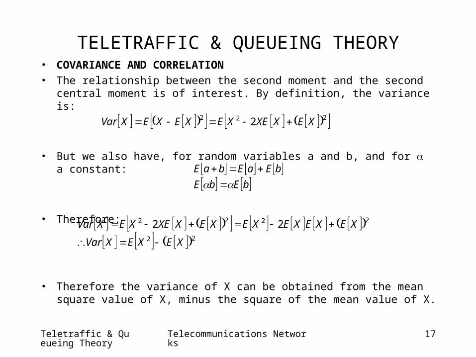
TELETRAFFIC & QUEUEING THEORY• COVARIANCE AND CORRELATION
• The relationship between the second moment and the second central moment is of interest. By definition, the variance is:
• But we also have, for random variables a and b, and for a constant:
• Therefore:
• Therefore the variance of X can be obtained from the mean square value of X, minus the square of the mean value of X.
222 2 XEXXEXEXEXEXVar
bEbE
bEaEbaE
22
2222 22
XEXEXVar
XEXEXEXEXEXXEXEXVar
Teletraffic & Queueing Theory
Telecommunications Networks 18
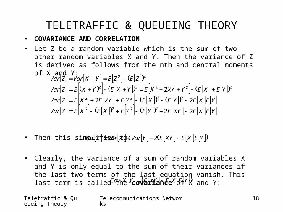
TELETRAFFIC & QUEUEING THEORY• COVARIANCE AND CORRELATION
• Let Z be a random variable which is the sum of two other random variables X and Y. Then the variance of Z is derived as follows from the nth and central moments of X and Y:
• Then this simplifies to:
• Clearly, the variance of a sum of random variables X and Y is only equal to the sum of their variances if the last two terms of the last equation vanish. This last term is called the covariance of X and Y:
YEXEXYEYEYEXEXEZVar
YEXEYEXEYEXYEXEZVar
YEXEYXYXEYXEYXEZVar
ZEZEYXVarZVar
22
22
2
2222
2222
22222
22
YEXEXYEYVarXVarZVar 2
YEXEXYEYXCov ,

Teletraffic & Queueing Theory
Telecommunications Networks 19
TELETRAFFIC & QUEUEING THEORY• COVARIANCE AND CORRELATION
• The covariance is a measure of the extent to which the corresponding random variables are correlated.
• We therefore find that:
• That means that if the covariance between X and Y is zero, then X and Y are uncorrelated.
• If X and Y are independent random variables, then they are uncorrelated.
YEXEXYEYXCov 0,

Teletraffic & Queueing Theory
Telecommunications Networks 20
TELETRAFFIC & QUEUEING THEORY• GENERATING FUNCTIONS
• There are many instances in practice when the quantity of interest is a sum of independent random variables.
• The mean and variance of such a sum can be obtained, as already shown, by adding together the means and variances, respectively, of the constituent variables.
• To find the CDF or PDF of a sum of random variables is, however, a more difficult task.
• If we have a sequence of numbers {f0,f1,f2,..fk,..}, the sequence can be converted into a single function to facilitate arithmetic manipulations. This process of converting a sequence of numbers into a single function is called z-transformation, and the resultant sequence is called the z-transform of the original sequence of numbers.
• The z-transform is commonly known as the generating function in probability theory.

Teletraffic & Queueing Theory
Telecommunications Networks 21
TELETRAFFIC & QUEUEING THEORY• GENERATING FUNCTIONS
• The z-transform of a sequence{fi} is defined as:
• The z-transform possesses some interesting properties which greatly facilitate the evaluation of parameters of a random variable. Let X and Y be two independent random variables with respective probability mass functions fk and gk; and let their corresponding z-transforms be F(z) and G(z). Then we have:
• Convolution property:
• If we define another random variable, H=F+G, with a probability mass function hk, then the z-transform H(z) of hk is given by:
0)(
k
kk zfzF
)()( zbGzaFbgaf kk
)()()( zGzFzH
Teletraffic & Queueing Theory
Telecommunications Networks 22
TELETRAFFIC & QUEUEING THEORY
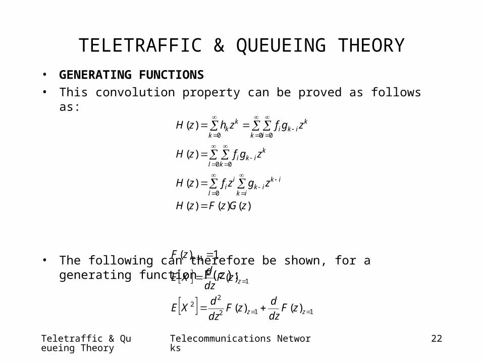
• GENERATING FUNCTIONS
• This convolution property can be proved as follows as:
• The following can therefore be shown, for a generating function F(z):
)()()(
)(
)(
)(
0
0 0
0 00
zGzFzH
zgzfzH
zgfzH
zgfzhzH
ik
ikik
l
ii
kik
l ki
kik
k ii
k
kk
112
22
1
1
)()(
)(
1)(
zz
z
z
zFdz
dzF
dz
dXE
zFdz
dXE
zF

Teletraffic & Queueing Theory
Telecommunications Networks 23
TELETRAFFIC & QUEUEING THEORY• PROBABILITY DISTRIBUTION FUNCTIONS
• Uniform Distribution
• Consider a continuous random variable, X, that is equally likely to take any value in a specified range. Such a variable is said to be uniformly distributed within that range.
• Also, since:
elsewhere
bxaforcxf
,0
,)(
abc
cdxdxxfb
a
1
1)(

Teletraffic & Queueing Theory
Telecommunications Networks 24
TELETRAFFIC & QUEUEING THEORY• PROBABILITY DISTRIBUTION FUNCTIONS
• Uniform Distribution
• The CDF is:
• The mean and variance of X are given by:
bxfor
bxaforab
ax
axfor
xF
duufxFx
,1
,
,0
)(
)()(
122
)(
2)((
222
222
abbadxxcXVar
XEXEdxxfXExXVar
badxxfxXE
b
a
Teletraffic & Queueing Theory
Telecommunications Networks 25
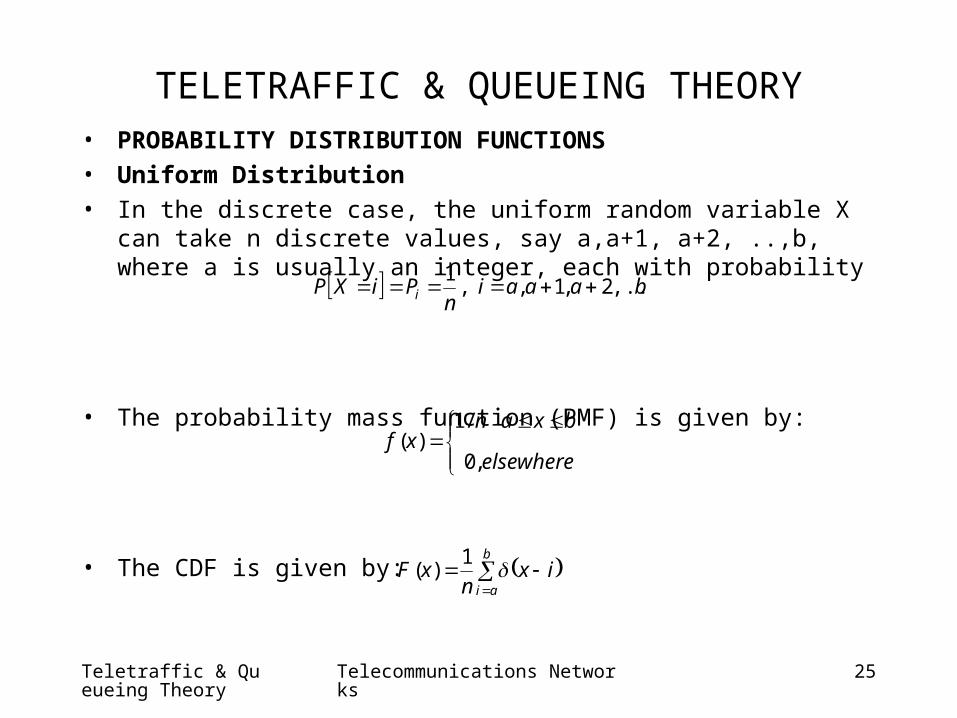
TELETRAFFIC & QUEUEING THEORY• PROBABILITY DISTRIBUTION FUNCTIONS
• Uniform Distribution
• In the discrete case, the uniform random variable X can take n discrete values, say a,a+1, a+2, ..,b, where a is usually an integer, each with probability
• The probability mass function (PMF) is given by:
• The CDF is given by:
baaain
PiXP i ,..,2,1,,1
elsewhere
bxanxf
,0
/1)(
b
aiix
nxF 1)(

Teletraffic & Queueing Theory
Telecommunications Networks 26
TELETRAFFIC & QUEUEING THEORY• PROBABILITY DISTRIBUTION FUNCTIONS
• To evaluate the mean and variance of the discrete uniformly distributed random variable, we note that the generating function is defined by:
• The variance is:
2
)1(
2
)1()(
..211)(
..11
)(/1
)(
1
1
2
1
0
n
n
nn
dz
zdFXE
nzzndz
zdF
zzzn
zn
zFnp
zpzF
z
n
nn
k
kk
k
kk
12
1
)1(..)3)(2(21
)(
)()(
2
22
2
112
22
22
nXVar
znnzn
zFdz
d
zFdz
dzF
dz
dXE
XEXEXVar
n
zz
Teletraffic & Queueing Theory
Telecommunications Networks 27
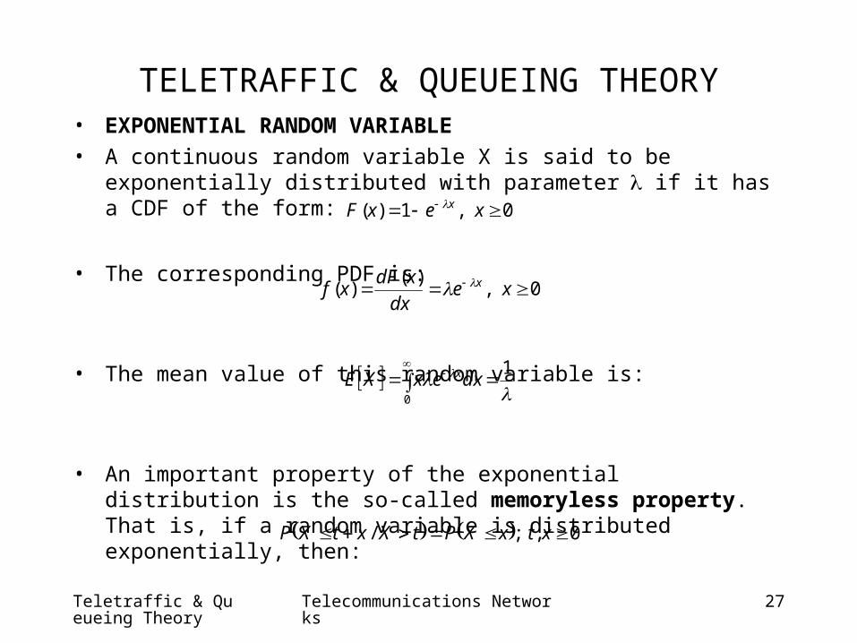
TELETRAFFIC & QUEUEING THEORY• EXPONENTIAL RANDOM VARIABLE
• A continuous random variable X is said to be exponentially distributed with parameter if it has a CDF of the form:
• The corresponding PDF is:
• The mean value of this random variable is:
• An important property of the exponential distribution is the so-called memoryless property. That is, if a random variable is distributed exponentially, then:
0,1)( xexF x
0,)(
)( xedx
xdFxf x
1
0
dxexXE x
0,;/ xtxXPtXxtXP
Teletraffic & Queueing Theory
Telecommunications Networks 28
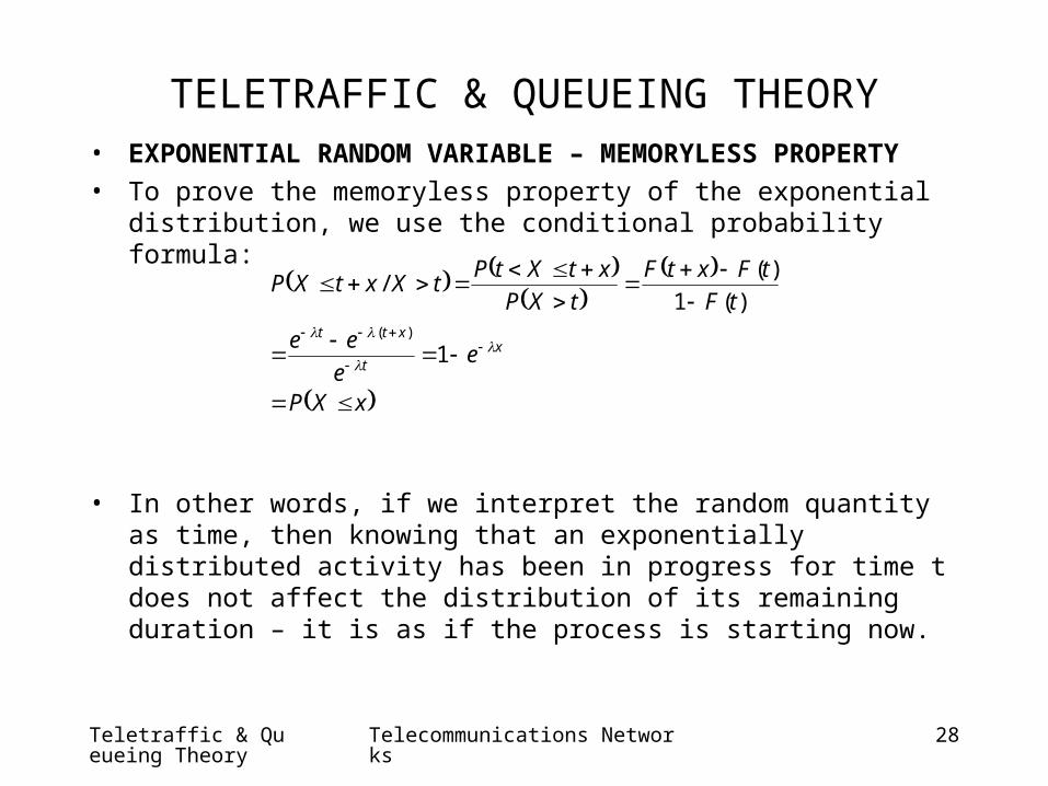
TELETRAFFIC & QUEUEING THEORY• EXPONENTIAL RANDOM VARIABLE – MEMORYLESS PROPERTY
• To prove the memoryless property of the exponential distribution, we use the conditional probability formula:
• In other words, if we interpret the random quantity as time, then knowing that an exponentially distributed activity has been in progress for time t does not affect the distribution of its remaining duration – it is as if the process is starting now.
xXP
ee
ee
tF
tFxtF
tXP
xtXtPtXxtXP
xt
xtt
1
)(1
)(/
)(
Teletraffic & Queueing Theory
Telecommunications Networks 29
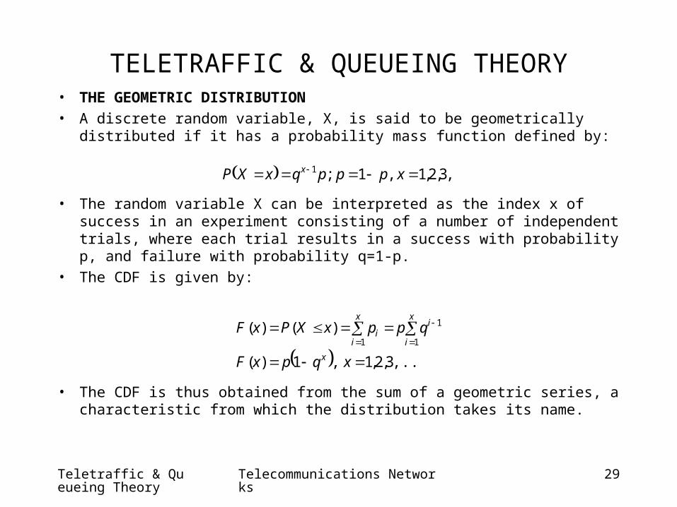
TELETRAFFIC & QUEUEING THEORY• THE GEOMETRIC DISTRIBUTION
• A discrete random variable, X, is said to be geometrically distributed if it has a probability mass function defined by:
• The random variable X can be interpreted as the index x of success in an experiment consisting of a number of independent trials, where each trial results in a success with probability p, and failure with probability q=1-p.
• The CDF is given by:
• The CDF is thus obtained from the sum of a geometric series, a characteristic from which the distribution takes its name.
,..3,2,1,1;1 xpppqxXP x
,..3,2,1,1)(
)()(1
1
1
xqpxF
qppxXPxF
x
x
i
ix
ii

Teletraffic & Queueing Theory
Telecommunications Networks 30
TELETRAFFIC & QUEUEING THEORY• THE GEOMETRIC DISTRIBUTION• The generating function of the random variable can be evaluated as:
• Then we can determine the mean and variance of X as:
• Just as the exponential distribution is the only continuous distribution that has the memoryless property, the geometric distribution is the only discrete distribution that has this same property. Because of this, both the geometric and exponential distributions have profound importance in queueing theory, especially in discrete and continuous Markov chains..
qz
pzzp
qzq
pqz
q
pzpqzp
i
i
i
ii
1)(
11
1)(
11
1
2
1
1
p
pXVar
pXE

Teletraffic & Queueing Theory
Telecommunications Networks 31
TELETRAFFIC & QUEUEING THEORY• BINOMIAL DISTRIBUTION
• A random variable X has a binomial distribution of order n if it takes the value 0,1,2,..,n with probability:
• The corresponding cumulative distribution function is a staircase in the interval [0,n], given by:
• The generating function of this random variable is:
• From this, we obtain the mean and variance of the binomial distribution as:
1;
qpqp
k
npkXP knk
k
1;)(0
mxmqpk
nxF
n
k
knk
nzpzR )1(1)(
)1( pnpXVar
npXE
Teletraffic & Queueing Theory
Telecommunications Networks 32
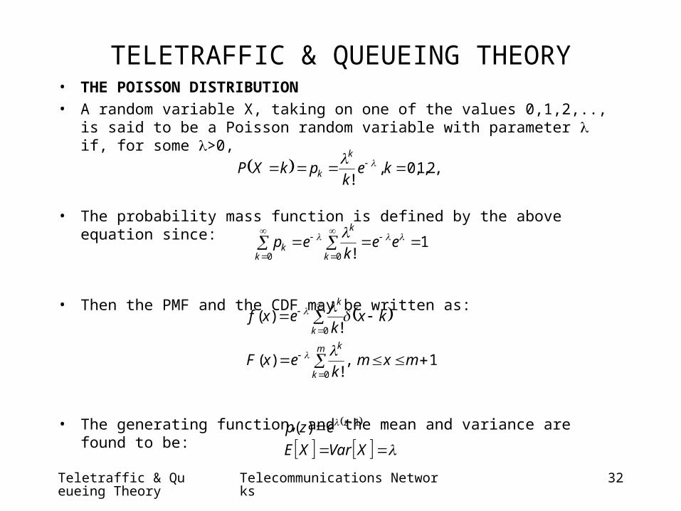
TELETRAFFIC & QUEUEING THEORY• THE POISSON DISTRIBUTION
• A random variable X, taking on one of the values 0,1,2,.., is said to be a Poisson random variable with parameter if, for some >0,
• The probability mass function is defined by the above equation since:
• Then the PMF and the CDF may be written as:
• The generating function, and the mean and variance are found to be:
,..2,1,0,!
kek
pkXPk
k
1!0 0
ee
kep
k k
k
k
1,!
)(
!)(
0
0
mxmk
exF
kxk
exf
m
k
k
k
k
XVarXE
ezp z 1)(
Teletraffic & Queueing Theory
Telecommunications Networks 33
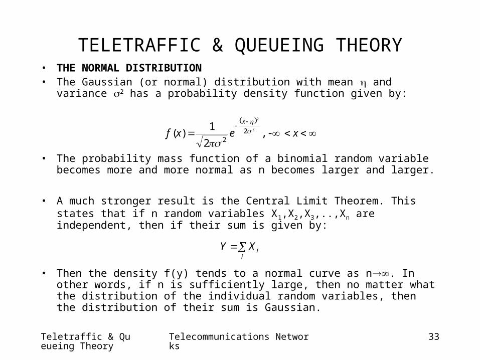
TELETRAFFIC & QUEUEING THEORY• THE NORMAL DISTRIBUTION• The Gaussian (or normal) distribution with mean and variance 2 has a
probability density function given by:
• The probability mass function of a binomial random variable becomes more and more normal as n becomes larger and larger.
• A much stronger result is the Central Limit Theorem. This states that if n random variables X1,X2,X3,..,Xn are independent, then if their sum is given by:
• Then the density f(y) tends to a normal curve as n. In other words, if n is sufficiently large, then no matter what the distribution of the individual random variables, then the distribution of their sum is Gaussian.
xexfx
,2
1)(
2
2
22
i
iXY