Tekoa Wastewater Treatment Plant Dissolved Oxygen, pH, …

Publication xx-xx-xxx i Month Year

Tekoa Wastewater Treatment Plant Dissolved Oxygen, pH, and Nutrients Receiving Water Study

May 2020

Publication 20-03-006

Publication Information This report is available on the Department of Ecology’s website at: https://fortress.wa.gov/ecy/publications/SummaryPages/2003006.html.

Data for this project are available in Ecology’s EIM Database. Study ID: tist0002.

The Activity Tracker Code for this study is 17-010.

Suggested Citation Stuart, T. 2020. Tekoa Wastewater Treatment Plant Dissolved Oxygen, pH, and Nutrients Receiving Water Study. Publication 20-03-006. Washington State Department of Ecology, Olympia. https://fortress.wa.gov/ecy/publications/SummaryPages/2003006.html.

Water Resource Inventory Area (WRIA) and 8-digit Hydrologic Unit Code (HUC) for the study area: WRIA 56; HUC 17010306.

Contact Information Publications Coordinator Environmental Assessment Program Washington State Department of Ecology P.O. Box 47600 Olympia, WA 98504-7600 Phone: 360-407-6764

Washington State Department of Ecology – https://ecology.wa.gov • Headquarters, Olympia 360-407-6000 • Northwest Regional Office, Bellevue 425-649-7000 • Southwest Regional Office, Olympia 360-407-6300 • Central Regional Office, Union Gap 509-575-2490 • Eastern Regional Office, Spokane 509-329-3400

Cover photo: Hangman Creek looking downstream from Lone Pine Rd., near Tekoa Wastewater Treatment Plant. Photo credit: Joe Joy.

Any use of product or firm names in this publication is for descriptive purposes only and does not imply endorsement by the author or the Department of Ecology.

To request ADA accommodation for disabilities, or printed materials in a format for the visually impaired, call the Ecology ADA Coordinator at 360-407-6831 or visit https://ecology.wa.gov/accessibility. People with impaired hearing may call Washington Relay Service at 711. People with speech disability may call 877-833-6341.

.

https://fortress.wa.gov/ecy/publications/SummaryPages/2003006.html

https://www.ecology.wa.gov/Research-Data/Data-resources/Environmental-Information-Management-database


https://ecology.wa.gov/

https://ecology.wa.gov/accessibility

Tekoa Wastewater Treatment Plant Dissolved Oxygen, pH, and Nutrients

Receiving Water Study

by

Tighe Stuart

Environmental Assessment Program Washington State Department of Ecology

Eastern Regional Office Spokane, Washington

This page is purposely left blank.

Tekoa WWTP DO, pH, and Nutrients Receiving Water Study Page 1

Table of Contents Page

List of Figures ...............................................................................................................2

List of Tables ................................................................................................................3

Acknowledgments ........................................................................................................4

Abstract .........................................................................................................................5

Introduction ..................................................................................................................6 Background ..............................................................................................................6 Study area description ..............................................................................................7 Beneficial uses and water quality standards ..........................................................11

Tekoa WWTP recommended nutrient limits ..........................................................12

Field Methods and Data Sources ..............................................................................13 Ecology data collection ..........................................................................................13 Non-Ecology data sources .....................................................................................18 Data quality ............................................................................................................18

Data Results and Discussion .....................................................................................19 pH, dissolved oxygen, and phytoplankton .............................................................19 Nutrients .................................................................................................................27 Streamflow, turbidity, and temperature .................................................................33

Modeling Analysis ......................................................................................................35 Analytical framework ............................................................................................35 Model calibration and assessment .........................................................................37 Model application ..................................................................................................40 Calculation of recommended effluent load limits ..................................................43

Conclusions and Recommendations .........................................................................45 Conclusions ............................................................................................................45 Recommendations ..................................................................................................45

References ...................................................................................................................46

Glossary, Acronyms, and Abbreviations .................................................................49

Appendices ..................................................................................................................53 Appendix A. Summary of data not available in EIM ............................................53 Appendix B. Data quality ......................................................................................60 Appendix C. Model inputs and calibration parameters .........................................72 Appendix D. Shade model .....................................................................................76 Appendix E. Determination of seasonal window for proposed effluent limits......78


List of Figures Page

Figure 1. Tekoa receiving water study area within the Hangman Creek watershed. ...........7

Figure 2. USGS stream-gage monthly flow statistics between 2007 and 2019 for Hangman Creek at state line (Gage ID 12422990). ............................................9

Figure 3. Land use patterns in and around the Tekoa receiving water study area. ............10

Figure 4. Map of Tekoa Receiving Water Study sampling locations. ...............................14

Figure 5. Daily maximum and minimum pH in upper Hangman Creek. ..........................21

Figure 6. Daily maximum and minimum dissolved oxygen (DO) in upper Hangman Creek. ................................................................................................................22

Figure 7. Continuous pH and DO in Hangman Creek above and below Tekoa WWTP. ..23

Figure 8. Measured and estimated phytoplankton (as chlorophyll a) in upper Hangman Creek. ................................................................................................................24

Figure 9. Relationship between phytoplankton (as Chlorophyll a) and daily maximum pH and DO. .......................................................................................................25

Figure 10. Phytoplankton bloom in Hangman Creek downstream of Tekoa WWTP, July 12, 2017. ....................................................................................................26

Figure 11. Soluble reactive phosphorus (SRP) in upper Hangman Creek. ........................28

Figure 12. Dissolved inorganic nitrogen (DIN) in upper Hangman Creek. .......................29

Figure 13. Streamflow upstream of Tekoa WWTP, and downstream effluent proportion. .........................................................................................................34

Figure 14. Turbidity and Temperature upstream of Tekoa WWTP. ..................................34

Figure 15. Conceptual diagram showing linkage of rTemp and RMA water quality models. ..............................................................................................................36

Figure 16. rTemp predicted and observed water temperatures ..........................................38

Figure 17. RMA predicted and observed DO and pH .......................................................39

Figure 18. Rank-sum distribution chart of all stream DIN values observed during the study. .................................................................................................................41


List of Tables Page

Table 1. Applicable water quality criteria for Hangman Creek. ........................................11

Table 2. Recommended effluent nutrient load limits for Tekoa WWTP. ..........................12

Table 3. Tekoa Receiving Water Study sampling locations. .............................................13

Table 4. Sample parameters and analytical methods. ........................................................15

Table 5. DIN:SRP ratios and nutrient limitation in upper Hangman Creek. .....................31

Table 6. SRP loads from Hangman Creek, Little Hangman Creek, and Tekoa WWTP. ..32

Table 7. DIN loads from Hangman Creek, Little Hangman Creek, and Tekoa WWTP. ..32

Table 8. Goodness-of-fit statistics for calibrated rTemp model ........................................37

Table 9. Goodness-of-fit statistics for calibrated RMA model ..........................................38

Table 10. RMA modeling scenario results. .......................................................................43


Acknowledgments The author of this report thanks the following people for their contributions to this study: • All of the landowners who granted permission to access their property to collect field data.

• City of Tekoa staff, including Kynda Browning and Duane Groom, for (1) their help with obtaining access to the wastewater treatment plant, (2) providing shorelines exemptions for gage station installation, and (3) all their efforts to improve sewer and wastewater operations and to protect water quality in Hangman Creek.

Washington State Department of Ecology staff: • Eiko Urmos-Berry for organizing and leading the field sampling effort. • Tyler Buntain and Mike McKay for gage station installation. • Mitch Wallace and Mike Anderson for gage station operation and streamflow measurement

support. • Andy Albrecht, Evan Newell, Brian Gallagher, Austin Stewart, Kayla Nowlin, and Steve

Hummel for assistance with the field study. • Manchester Environmental Laboratory staff including Nancy Rosenbower and Leon Weiks. • Elaine Snouwaert and Mitch Redfern, Water Quality Program basin leads. • Kimberly Prisock, Water Quality Program permit manager for Tekoa WWTP. • George Onwumere and Cathrene Glick for their support as EAP managers. • Jimmy Norris and Joan LeTourneau for editing, formatting, and publishing the report.


Abstract The City of Tekoa, located near the Idaho border south of Spokane, operates a wastewater treatment plant (WWTP), which discharges to Hangman Creek. The WWTP was constructed in 1950, with significant upgrades in 1974 and 1990. Aging facility infrastructure and a compliance schedule for effluent temperature limits from the Hangman Creek Watershed Fecal Coliform, Temperature, and Turbidity Total Maximum Daily Load (Joy et al., 2009) have created a need for facility upgrade or replacement. Preliminary data from 2009 also suggested that Tekoa WWTP’s discharge of nutrients affects downstream pH and dissolved oxygen (DO) in Hangman Creek.

To determine the effluent nutrient load limits needed to protect pH and DO in Hangman Creek, and to provide the information needed for Tekoa’s facility planning efforts, Ecology undertook a receiving water field study during May-October 2017. The study focused on nutrients, pH, dissolved oxygen, and algal eutrophication. We found consistent impacts to pH and DO downstream of Tekoa WWTP during the summer months. An effluent-fed phytoplankton bloom during July 2017 resulted in high algae concentrations and pH in excess of the 8.5 S.U. water quality standard.

We used the rTemp and River Metabolism Analyzer (RMA) model frameworks to assess the sensitivity of pH and DO in Hangman Creek to nutrients. We calculated proposed effluent load limits for Tekoa WWTP of 0.0132 kg/d (0.0291 lbs/d) dissolved inorganic nitrogen (DIN) and 0.00183 kg/d (0.00404 lbs/d) total phosphorus (TP). These limits are applicable each year during June through October. We also emphasize the need, indicated by the 2009 multiparameter TMDL, to restore riparian vegetation along Hangman Creek. In addition to lowering temperatures, this will improve pH and dissolved oxygen.


Introduction Background Tekoa is a farming community with a population of about 800, located in Whitman County near the Idaho border. It is in the upper part of the Hangman Creek watershed, at the confluence of Little Hangman and Hangman Creeks.

The City of Tekoa owns and operates a wastewater treatment plant (WWTP), which discharges effluent to Hangman Creek. The original facility consisting of a single stage trickling filter system was constructed in 1950, with major modifications occurring in 1974 to convert the plant to an activated sludge system with chlorine disinfection. The city made additional improvements to the WWTP in 1990, adding a new lift station, drying beds for biosolids storage, and installation of a dechlorination system. The facility infrastructure is aging and is need of significant repair, upgrade, or replacement.

In addition, the Hangman Creek Watershed Fecal Coliform, Temperature, and Turbidity Total Maximum Daily Load (Joy et al., 2009) established temperature wasteload allocations for Tekoa WWTP that require effluent temperature reductions during June, July, and August. Tekoa is currently on a compliance schedule to meet those requirements, and will be required to meet the final temperature limits by July 2024, presenting further imperative for facility upgrades.

Preliminary data collected during 2009 suggested that nutrients in Tekoa WWTP’s effluent might be contributing to dissolved oxygen (DO) and/or pH impairments in Hangman Creek, and that nutrient reduction or elimination might be needed to meet water quality standards for DO and pH (Joy, 2008; Ross, 2011).

Without a wasteload allocation from a DO/pH Total Maximum Daily Load study (TMDL), the municipal permit team requested support from Ecology’s Environmental Assessment Program (EAP) in collecting data that would (1) support the development of permit limits for nutrients that are protective of water quality and (2) allow the City of Tekoa to move forward with necessary facility planning efforts.

This report presents the findings of Ecology’s 2017 field study, provides a modeling analysis of the impacts of effluent nutrients on the receiving water, and recommends effluent nutrient limits for Tekoa WWTP.


Study area description Hangman Creek is a major tributary to the Spokane River. Its watershed drains approximately 692 square miles in two states and four counties. The Tekoa DO, pH, and Nutrients Receiving Water Study area is in the uppermost part of the watershed inside of Washington, encompassing about 12 river miles between the state line and the town of Latah (Figure 1).

Figure 1. Tekoa receiving water study area within the Hangman Creek watershed.


Geological setting Bedrock in the Tekoa area of the Hangman watershed is mainly Miocene basalt flows, along with the siltstones and sandstones of the Latah Formation. Buttes such as Tekoa Mountain are formed from Precambrian siltite and quartzite islands jutting above the basalt flows. Soils consist of wind-blown silt, or loess, which accumulated from Pleistocene glacial deposits and forms the characteristic dune-shaped hills of the Palouse region (Waggoner, 1990).

The loess soils of the Palouse region are highly erodible. As a result, Hangman Creek is susceptible to bank erosion. These soil characteristics combined with human activities have contributed to the wide channels and deep, slow pools that typify stream channel morphology in upper Hangman Creek. Each year during the spring runoff season, Hangman Creek transports large amounts of loess sediment originating from bank and field erosion.

Hydrology Hangman Creek at Tekoa represents a drainage area of about 197 square miles (including Little Hangman Creek), or about 28% of the entire Hangman watershed. Figure 2 illustrates streamflow patterns at the nearest USGS gaging station to Tekoa, located at the state line (upstream of Little Hangman Creek, and about 4 miles upstream of Tekoa WWTP; Gage ID 12422990). The spring runoff period typically occurs between January and May. Flows drop quickly between April and July, with the baseflows occurring during August and September. A wide seasonal variation in flows exists in Hangman Creek, with typical March flows over 400 times higher than typical flows during September. Flows during the spring runoff period are very “flashy,” exhibiting a quick response to precipitation and snowmelt events. Peak flows in excess of 2,000 cfs occasionally occur.


Figure 2. USGS stream-gage monthly flow statistics between 2007 and 2019 for Hangman Creek at state line (Gage ID 12422990).


Land use Figure 3 shows land use in the Tekoa area. Dryland agriculture dominates land use in this portion of the Hangman watershed. Forest and open grassland areas occur on Tekoa Mountain, a prominent butte north of Hangman Creek between Tekoa and Latah. Urban development is mainly restricted to the communities of Tekoa and Latah.

Figure 3. Land use patterns in and around the Tekoa receiving water study area. Source: USGS Land Use/Land Cover (GIRAS).


Beneficial uses and water quality standards This study addresses the protection of aquatic habitat and attainment of the aquatic life uses in the upper portion of Hangman Creek within Washington. According to watershed assessments of current and historical fish populations (SCD, 2005):

Fish habitat and distribution throughout the watershed has radically changed over the last one hundred years. Hangman Creek once had viable populations of native redband trout and healthy runs of salmon and steelhead. The removal of riparian vegetation, channel alterations, and heavy sedimentation has significantly reduced the spawning and rearing habitat on Hangman Creek. The primary species now found in the stream are adapted to warmer, slower waters and considered undesirable as gamefish. Resident trout populations are severely depressed.

The portion of Hangman Creek within the study area no longer supports redband trout (Western Native Trout Initiative, 2007; Lee, 2005). Lee (2005) did not find any salmonids in Hangman Creek between Latah and the state line, in Cove Creek, or in Little Hangman Creek. (Some parts of the lower watershed still do support salmonids.) Improving water quality conditions is a necessary step to protect and restore the aquatic community, including cold-water fisheries on which the water quality standards are based in this watershed. Proper DO and pH levels are essential for healthy fish and macroinvertebrate populations.

In the Washington State water quality standards, freshwater aquatic life use categories are described using key species (salmonid versus warm-water species) and life-stage conditions (spawning versus rearing). The designated use for Hangman Creek is “Salmonid Spawning, Rearing, and Migration,” which reflects the historical presence of salmonids and a shared desire among managers, stakeholders, and citizen groups to restore Hangman Creek to a state where it could again support these species.

Table 1 summarizes the DO and pH water quality criteria associated with the “Salmonid Spawning, Rearing and Migration” use applicable to Hangman Creek.

Table 1. Applicable water quality criteria for Hangman Creek.

Parameter Criteria

Dissolved Oxygen

DO concentration will not fall below 8.0 mg/L more than once every ten years on average. When a water body's DO is lower than 8.0 mg/L (or within 0.2 mg/L) and that condition is due to natural conditions, then human actions considered cumulatively may not cause the DO of that water body to decrease more than 0.2 mg/L.

pH pH shall be within the range of 6.5 to 8.5 with a human-caused variation within above range of less than 0.5 units.


Tekoa WWTP recommended nutrient limits Ecology is recommending effluent nutrient load limits for Tekoa WWTP for nitrogen and phosphorus. The load limits for nitrogen are expressed in terms of dissolved inorganic nitrogen (DIN), which is the sum of nitrate+nitrite+ammonia. The load limits for phosphorus are expressed in terms of total phosphorus (TP). These load limits are very restrictive, representing only a small fraction of the nutrient loads that Tekoa WWTP currently discharges. Table 2 presents the recommended nutrient load limits. The remainder of this report presents the methodology, data, modeling, analysis, and rationale for these limits.

Table 2. Recommended effluent nutrient load limits for Tekoa WWTP.

Parameter Recommended effluent load limit (kg/d)

Recommended effluent load limit (lbs/d)

Nitrogen (DIN) 0.0132 0.0291

Phosphorus (TP) 0.00183 0.00404

Critical season when nutrient limits apply: June - October


Field Methods and Data Sources Ecology data collection Ecology collected field data in upper Hangman Creek during May-October of 2017. This data collection effort followed a project-specific Quality Assurance Project Plan (QAPP; Albrecht et al., 2017) as well as Ecology’s programmatic QAPP for water quality impairment studies (McCarthy and Mathieu, 2017). Our analysis also used some data from earlier field studies in the Hangman Creek watershed during 2008-2009 (Joy, 2008; Ross, 2011) and during 2016 (Stuart, 2016). Table 3 lists the sampling locations and the types of data that we collected at each location. Figure 4 shows a map of the sampling locations.

Table 3. Tekoa Receiving Water Study sampling locations.

Study Specific Location ID Sampling Location Latitude Longitude

Nut

rient

s

Chl

orop

hyll

a

Perip

hyto

n bi

omas

s (2

009)

Con

tinuo

us s

tream

flow

Dis

cret

e st

ream

flow

Con

tinuo

us tu

rbid

ity

Con

tinuo

us w

ater

qua

lity

sond

e

Die

l wat

er q

ualit

y so

nde

Con

tinuo

us w

ater

tem

pera

ture

Con

tinuo

us a

ir te

mp

& de

w p

oint

Hem

isph

eric

al ri

paria

n ph

otos

Long

itudi

nal d

epth

(201

6)

Tim

e of

trav

el

56HAN-58.5 Hangman Ck. at State Line 47.2028 -117.0406 2x X U X X S X L

56HAN-56.3 Hangman Ck. nr Tekoa Golf Course 47.2172 -117.0630 X X X X L

56HAN-55.1 Hangman Ck. abv Little Hangman Ck. 47.2220 -117.0755 2x G X G X S X L T

56LIT-00.1 Little Hangman Ck. at Connell St. 47.2254 -117.0747 2x G X G X S

56HAN-54.7 Hangman Ck. at rodeo grounds 47.2245 -117.0788 X P X X P X L T

56TEKWTP Tekoa WWTP effluent 47.2277 -117.0829 X D X S X

56HAN-54.3 Hangman Ck. below Tekoa 47.2290 -117.0859 X X X P X X P X L T

56HAN-53.8 Hangman Ck. far below Tekoa 47.2271 -117.0950 X X X X S X L T

56HAN-50.5 Hangman Ck. at Fairbanks Rd. 47.2417 -117.1326 X X L

56HAN-47.0 Hangman Ck. at Marsh Rd. 47.2760 -117.1525 X P X X P X L

56COV-00.2 Cove Ck. at mouth 47.2787 -117.1532 2x P X X P

56HAN-46.3 Hangman Ck. at Spring Valley Rd. 47.2817 -117.1616 X X X X L All data collected during 2017 unless otherwise noted. 2x – Nutrient samples collected twice per month. U – USGS streamflow gaging station. G – Ecology streamflow gaging station with continuous turbidity. P – Continuous streamflow and temperature measured using pressure transducers. D – Facility reported effluent flow data in discharge monitoring reports, combined with pressure transducer data. S – Temperature recorded by continuous water quality sonde. L – Longitudinal depth recorded continuously along Hangman Creek (not just at sampling locations). T – Time of travel measured along Hangman Creek for all reaches between 56HAN-55.1 and 56HAN-53.8.


Figure 4. Map of Tekoa Receiving Water Study sampling locations.


Nutrients During 2017, Ecology collected water samples monthly at all sampling locations and twice monthly at four of these locations. At stream sampling locations, we collected grab samples from the thalweg in a well-mixed part of the channel. At Tekoa WWTP, we collected 24-hour composite samples from the effluent sluice using an ISCO® compositor. Ecology’s Manchester Environmental Laboratory (MEL) analyzed all samples for this study. Table 4 lists the sample parameters and analytical methods.

Table 4. Sample parameters and analytical methods.

Parameter Method

Total Persulfate Nitrogen SM 4500-NB Ammonia SM 4500-NH3 -H Nitrate/Nitrite SM 4500-NO3 -I Total Phosphorus SM 4500-P H Orthophosphate (Soluble Reactive Phosphorus)* SM 4500-P G Total Organic Carbon SM 5310B Dissolved Organic Carbon SM 5310B Total Suspended Solids SM 2540D Total Non-Volatile Suspended Solids EPA 160.4 Alkalinity SM 2320B Chloride EPA 300.0 Chlorophyll a ** SM 10200H3 Biochemical Oxygen Demand 5-day SM 5210B

SM = Standard Methods for the Examination of Water and Wastewater, 20th Edition (APHA, 2005; ASTM, 1997). EPA = EPA Method Code. * Manchester Environmental Laboratory refers to this parameter as orthophosphate. It is commonly referred to as soluble reactive phosphorus (SRP), and that is how we refer to it in this report. ** Parameter collected only at a subset of sampling locations and dates.

Streamflow Ecology’s Environmental Assessment Program Freshwater Monitoring Unit (FMU) installed two stream gaging stations at 56HAN-55.1 (Hangman Creek above Little Hangman Creek) and 56LIT-00.1 (Little Hangman Creek at Connell St.). We also installed Hobo® stand-alone pressure transducers at four additional locations. These stations recorded stage height continuously through the study period. We measured flow and stage approximately twice monthly at these locations, and used the measured relationship between stage and flow to convert the continuous stage record into a continuous flow record.

At the remaining stream sampling locations, we measured flow monthly, concurrently with water sample collection. The two exceptions to this were 56HAN-58.5 (Hangman Creek at state line), where we used continuous flow data collected by the U.S. Geological Survey (USGS), and 56HAN-50.5 (Hangman Creek at Fairbanks Rd.), where we did not have landowner permission to access the stream banks outside the public road right-of-way.


Continuous water quality and turbidity At six locations, Ecology deployed Hydrolab® multiprobe sondes continuously throughout the study period to record dissolved oxygen, pH, temperature and conductivity. The sondes logged measurements of these parameters every 15 minutes. At the remaining six locations, we deployed Hydrolab® and/or YSI EXO® sondes to record these same parameters for an approximately 48-hour period during each monthly sampling survey. We also collected routine spot measurements of these parameters as a QC check on the deployed instruments.

We collected continuous turbidity throughout the study period at the two FMU gaging stations using FTS® DTS-12 turbidity sensors. We also collected routine spot turbidity measurements using a Hach® portable turbidity meter as a QC check on the station sensors.

Hydraulic geometry and time-of-travel Stream channel width, depth, and velocity have an important influence on the response of DO and pH to instream biological processes and on the downstream transport of nutrients and other substances.

To assess the widths of Hangman Creek, we digitized the wetted banks from 2017 12-inch resolution National Agriculture Imagery Program (NAIP) color orthophotos (aerial photographs geometrically corrected to have the same scale as a map). We calculated wetted widths every 10 meters using the TTools extension for ArcGIS (Ecology, 2015). TTools is a GIS-based tool used for spatial analysis of stream channels and riparian areas, including vegetation and shade.

We collected water depth data for the entirety of Hangman Creek within Washington during April 2016, including the Tekoa Receiving Water Study area. To measure water depths, we mounted a Hydrolab® Minisonde® equipped with a depth probe snugly inside a length of PVC pipe and dragged it along the bottom of the channel behind a canoe. A Surveyor® deck unit equipped with GPS recorded location coordinates and a corresponding depth measurement every 30 seconds.

To assess water velocities, we conducted two time-of-travel studies on June 19 and August 14-18, 2017 to represent two different flow conditions. The time-of-travel studies used rhodamine, a fluorescent, non-toxic tracer dye, to estimate travel times by measuring the time it takes for a slug of the dye to reach specific downstream locations. During both studies, we assessed travel times for the reach between 56HAN-55.1 (Hangman Creek above Little Hangman Creek) and 56HAN-53.8 (Hangman Creek far below Tekoa).


Periphyton and Phytoplankton

Periphyton Periphyton consists of a community of algae, fungi, microbes, and microscopic plants and animals that grow in shallow water habitats attached to submerged surfaces. Periphyton productivity is often one of the most important drivers of DO and pH in shallow streams and rivers.

Ecology collected periphyton biomass samples on June 22 and July 27, 2009 at 56HAN-58.5 (Hangman Creek at state line) and 56HAN-54.3 (Hangman Creek below Tekoa) using a modified version of USGS protocols (Porter et al., 1993; Mathieu et al., 2013). At each site, we collected three representative rocks from the streambed. We scraped periphyton from the rocks into the sample container along with deionized water. Ecology’s Manchester Environmental Laboratory analyzed the samples for Chlorophyll a and Ash-Free Dry Weight. We then calculated areal periphyton biomass as the total quantity of Chlorophyll a or Ash-Free Dry Weight collected divided by the rock surface area from which we had scraped the periphyton. Ash-Free Dry Weight represents total biomass, while Chlorophyll a represents photosynthetic biomass.

Phytoplankton Phytoplankton are algae, photosynthetic bacteria, and protists that are suspended in the water column. In most shallow streams and rivers, phytoplankton are not an important driver of DO and pH. However, because downstream advective transport is extraordinarily slow in Hangman Creek during the summer months, phytoplankton blooms can occur and persist in Hangman Creek. To assess critical-season phytoplankton activity in the reach downstream of Tekoa WWTP, Ecology collected water samples for Chlorophyll a at 56HAN-54.3 (Hangman Creek below Tekoa) and 56HAN-53.8 (Hangman Creek far below Tekoa) during July, August, and September 2017.

Continuous water and air temperature Ecology obtained continuous water temperature data from deployed instrumentation including the FMU gage stations, Hobo® pressure transducers, and Hydrolab® multiprobe sondes. We used spot temperature measurements taken with Hydrolab® sondes as QC checks on the continuous temperature records from all instrument types.

To measure local air temperature and dew point, we deployed a Hobo® RH/Temp datalogger on the grounds of Tekoa WWTP for the duration of the study period.


Hemispherical riparian photography We measured effective shade by taking hemispherical riparian vegetation photographs at most mainstem Hangman Creek sampling locations during August 2017. We took photographs from the center of the wetted channel. We analyzed hemispherical photographs using Gap Light Analyzer (GLA) canopy analysis software (Frazer et al., 1999).

Non-Ecology data sources USGS Flow The U.S. Geological Survey (USGS) operates a continuous streamflow gauging station on Hangman Creek at the state line (Station ID 12422990).1 This is the same location as the sampling site 56HAN-58.5 in this study. This gage has been in operation since 2007.

Meteorology For temperature modeling, we used wind speed and solar radiation data from the interagency Remote Automatic Weather Station (RAWS) located at Turnbull National Wildlife Refuge (ID TWRW1), about 25 miles northwest of the study area. RAWS stations are operated by jointly by agencies including the National Interagency Fire Center (NIFC), the National Oceanic and Atmospheric Administration (NOAA), and the Western Regional Climate Center (WRCC).

For analysis of seasonal weather trends and statistics, we used air temperature data from the NOAA National Weather Service (NWS) weather station at Spokane Airport (ID KGEG), the nearest location with a long-term climate record.

Data quality We assessed the quality of all data collected and used in this study. Appendix B provides the details of this data quality assessment. All data are of adequate quality to their intended use in this project. We have taken data quality and qualifications into account in developing results and recommendations.

1 Data are available at https://waterdata.usgs.gov/wa/nwis/uv/?site_no=12422990&agency_cd=USGS

https://waterdata.usgs.gov/wa/nwis/uv/?site_no=12422990&agency_cd=USGS


Data Results and Discussion Data from the Tekoa Receiving Water Study are available at Ecology’s Environmental Information Management (EIM) website at https://fortress.wa.gov/ecy/eimreporting/Default.aspx. Search User Study ID: tist0002. A few data types not supported by EIM are presented in Appendix A.

The data collected during the Tekoa Receiving Water Study illustrate the spatial and temporal patterns of pH, dissolved oxygen (DO), and algal eutrophication in upper Hangman Creek. They also provide insight into the causal links between nutrients, algae growth, pH, and DO.

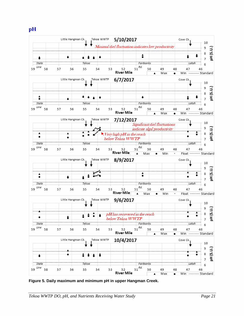
pH, dissolved oxygen, and phytoplankton Figures 5-7 present observed pH and DO in upper Hangman Creek. Figures 5-6 show daily maximum and minimum pH and DO graphed longitudinally (along the length of the stream). For the July and August surveys, the graphs show additional data between 56HAN-54.3 (Hangman Creek below Tekoa WWTP) and 56HAN-53.8 (Hangman Creek far below Tekoa WWTP). During each of these surveys, we floated the reach between these two sites once in the morning (near the daily minimums for pH and DO) and once in the afternoon (near the daily maximums) collecting measurements along the entire distance. Figure 7 presents continuous pH and DO data at 56HAN-55.1 (Hangman Creek above Little Hangman Creek), which is upstream of both Little Hangman Creek and Tekoa WWTP, and 56HAN-53.8 (Hangman Creek far below Tekoa WWTP), which is about 0.6 mile downstream of Tekoa WWTP, near the point where the wastewater discharge has its maximum impact on the receiving water.

During summer, pH and DO in Hangman Creek exhibit diel fluctuations, or “swings,” with high pH and DO during late afternoon and low pH and DO during early morning (Figure 7). This pattern is characteristic of slow-moving streams with ample algal productivity. During daylight hours, algae and aquatic plant (macrophyte) photosynthesis outpaces respiration. When this happens, DO increases in the water column. At the same time, the photosynthesis depletes dissolved carbon dioxide, raising the pH of the water. At night, the opposite happens – photosynthesis ceases and respiration dominates, depleting DO and at the same time increasing dissolved carbon dioxide, which reduces pH. This pattern was ubiquitous during the warm summer months. However, diel fluctuations were small during the very beginning and end of our study period (early May and late October) “shoulder seasons.”

Figure 8 presents observed phytoplankton (suspended algae) represented as instream chlorophyll a. We collected chlorophyll a samples at the two sites downstream of Tekoa WWTP during July, August, and September. At other locations and times, the data shown represent estimates derived from a regression between chlorophyll a and organic suspended solids (OSS; equivalent to total suspended solids minus total non-volatile suspended solids). Figure 9 shows photographs of Hangman Creek in the long pool downstream of Tekoa WWTP during a phytoplankton bloom in early July.

https://fortress.wa.gov/ecy/eimreporting/Default.aspx


Our study found that suspended algae, or phytoplankton, play a key role in determining summertime pH and DO levels in upper Hangman Creek. There is a positive correlation in our dataset between high Chlorophyll a and high pH/DO. This is particularly true in the reach downstream of Tekoa WWTP (Figure 9). On July 12, 2017, we observed a sharp increase in Chlorophyll a concentrations between 56HAN-54.3 (about 0.1 mile downstream of the WWTP outfall) and 56HAN-53.8 (about 0.6 mile downstream). Chlorophyll a concentrations reached 74.9 ug/L at the further downstream site (Figure 8). This is a high value, resulting in the stream taking on an opaque, pea-soup colored appearance (Figure 10).

This phytoplankton bloom corresponded with very high pH and DO during early July (Figure 7), resulting in a violation of water quality standards for pH. We observed the same pattern downstream of Tekoa WWTP during August, but to a lesser extreme. Other violations of pH criteria observed during the study also appear related to phytoplankton. For example, during October, we observed both high phytoplankton levels and high pH at 56HAN-56.3 (Hangman Creek at Tekoa Golf Course), possibly the result of an intermittent non-point nutrient source.

It is somewhat unusual for phytoplankton to play such a key role in eutrophication issues in a small stream system like upper Hangman Creek. More commonly, it is attached algae (periphyton) or aquatic plants (macrophytes) that drive pH and DO fluctuations in such streams. Periphyton and macrophytes are present in upper Hangman Creek and likely play a role. For example, Figure 9 shows that there were some times and places when low chlorophyll a concentrations coincided with daily max pH near 8.5 and daily max DO > 12 mg/L. These instances may reflect periphyton activity. However, phytoplankton apparently are the primary driver of excessive pH and very high DO. This probably has to do with the extraordinarily slow (<0.01 ft/s) movement of water through deep (3ft+), wide (40ft+) pools during the summertime, allowing ample time for phytoplankton to grow and multiply before being transported out of the system.


pH

Figure 5. Daily maximum and minimum pH in upper Hangman Creek.


Dissolved Oxygen

Figure 6. Daily maximum and minimum dissolved oxygen (DO) in upper Hangman Creek.


Figure 7. Continuous pH and DO in Hangman Creek above and below Tekoa WWTP.


Phytoplankton (suspended algae)

Figure 8. Measured and estimated phytoplankton (as chlorophyll a) in upper Hangman Creek.


Figure 9. Relationship between phytoplankton (as Chlorophyll a) and daily maximum pH and DO.


Figure 10. Phytoplankton bloom in Hangman Creek downstream of Tekoa WWTP, July 12, 2017.


Nutrients Figure 11 presents observed Soluble Reactive Phosphorus (SRP) in upper Hangman Creek. Figure 12 presents Dissolved Inorganic Nitrogen (DIN). SRP and DIN are the inorganic forms of phosphorus and nitrogen that are readily available for uptake by algae. During May and June, SRP and DIN levels were fairly uniform throughout, and elevated in the case of DIN. This is because of higher flows and greater dilution of individual sources. During low flow, DIN levels drop due to algal uptake of nitrogen and the loss of the constant supply that high flows provide. SRP and DIN patterns clearly show the effect of localized sources. SRP and DIN increase downstream of Tekoa WWTP as a result of the wastewater nutrient load. Progressing downstream from Tekoa WWTP, the concentrations decrease again as algae take up dissolved nutrients into their cells.

Tekoa WWTP is the predominant source of SRP in upper Hangman Creek, and the only one clearly visible in Figure 11. However, there are other large sources of DIN visible in Figure 12, including Little Hangman Creek and Cove Creek.


Soluble Reactive Phosphorus (SRP)

Figure 11. Soluble reactive phosphorus (SRP) in upper Hangman Creek.


Dissolved Inorganic Nitrogen (DIN)

Figure 12. Dissolved inorganic nitrogen (DIN) in upper Hangman Creek.


Nutrient limitation The relative importance of nitrogen vs. phosphorus, or nutrient limitation, can be evaluated using the ratios of DIN to SRP. Whichever nutrient is in shorter supply relative to algal demand, will be potentially limiting. Ratios of DIN to SRP of less than 4.5:1 indicate nitrogen limitation, ratios over 9:1 indicate phosphorus limitation, while ratios between 4.5:1 and 9:1 are uncertain (Borchardt, 1996).2 Table 5 presents DIN:SRP ratios in upper Hangman Creek observed during May-October 2017. Potentially phosphorus-limited conditions prevail during higher flows when nitrogen is in greater supply, although in reality, the cold, turbid water found during those times probably means that temperature and/or light, not nutrients, limits algae growth. During the low-flow period, nitrogen-limited conditions prevail.

Although nitrogen is the primary limiting nutrient for addressing eutrophication issues during the low-flow period, co-limitation may occur and phosphorus may be relevant. For example, if Tekoa WWTP eliminated all phosphorus, but not nitrogen, from its effluent, the downstream DIN:SRP ratio during July-September 2017 might have varied from 7.9 – 23.4, a range of values indicative of phosphorus-limitation3. In other words, although nitrogen is primarily limiting, phosphorus may be secondarily limiting. Reductions in both nitrogen and phosphorus are important to controlling algae growth downstream of Tekoa WWTP.

2 Ratios here are expressed as mass (mgN/L:mgP/L). These ratios are often expressed as molar ratios, including in the reference literature. Molar N:P ratios of 10:1 or less indicate nitrogen limitation, ratios over 20:1 indicate phosphorus limitation, and ratios between 10:1 and 20:1 are uncertain. 3 We estimated these values as the ratio of observed SRP above the WWTP (56HAN-54.7) to DIN below the WWTP (56HAN-54.3).


Table 5. DIN:SRP ratios and nutrient limitation in upper Hangman Creek.

Location Description Site ID

DIN:SRP (as mass)

5/10

/201

7

6/7/

2017

7/12

/201

7

8/9/

2017

9/6/

2017

10/4

/201

7

Mainstem Hangman Creek Locations Hangman Ck. at state line 56HAN-58.5 69 37 22 1.8 3.0 85 Hangman Ck. at golf course 56HAN-56.3 54 39 8.1 1.3 3.4 1.0 Hangman Ck. abv Little Hangman Ck. 56HAN-55.1 52 37 1.8 1.0 2.5 1.7 Hangman Ck. at rodeo grounds 56HAN-54.7 52 36 4.9 2.1 2.0 15 Hangman Ck. below Tekoa 56HAN-54.3 45 29 2.7 2.2 2.7 7.7 Hangman Ck. far below Tekoa 56HAN-53.8 48 31 0.2 0.5 2.5 8.8 Hangman Ck. at Fairbanks Rd. 56HAN-50.5 45 37 0.4 16 0.6 2.7 Hangman Ck. at Marsh Rd. 56HAN-47.0 46 34 0.7 0.5 0.5 0.6 Hangman Ck. at Spring Valley Rd. 56HAN-46.3 44 34 8.7 13 25 26

Tributary and Source Locations Little Hangman Ck. at Connell St. 56LIT-00.1 51 31 0.5 0.3 0.4 23 Tekoa WWTP effluent1 56TEKWTP 4.0 5.0 1.3 3.0 3.0 6.1 Cove Ck. at mouth 56COV-00.2 37 29 33 37 39 50 Blue = P-limited Yellow = N-limited Green = uncertain

1 It is not strictly correct to refer to the “nutrient limitation” of wastewater, since an effluent stream is not a water body. However, the wastewater nutrient ratios are informative with respect to the wastewater nutrient contribution to the receiving water.


Nutrient contribution from Tekoa WWTP Tables 6-7 present the SRP and DIN load contributions of Hangman Creek above Little Hangman Creek, Little Hangman Creek, and Tekoa WWTP. During the “shoulder seasons” (May and late October), Tekoa WWTP contributes a minority of SRP (<30%) and a negligible proportion of DIN (<5%). However, during the low-flow period, Tekoa WWTP contributes the vast majority (at times >90%) of both SRP and DIN.

Table 6. SRP loads from Hangman Creek, Little Hangman Creek, and Tekoa WWTP. SRP Load (kg/day) SRP Load (% of total1)

Date

Hangman Creek abv

LHC (56HAN-55.1)

Little Hangman

Creek (56LIT-00.1)

Tekoa WWTP effluent

(56TEKWTP)

Hangman Creek abv

LHC (56HAN-55.1)

Little Hangman

Creek (56LIT-00.1)

Tekoa WWTP effluent

(56TEKWTP)

5/10/2017 4.7 1.6 1.0 64% 22% 14% 5/24/2017 4.1 1.0 0.77 69% 18% 13%

6/7/2017 1.8 0.78 0.55 57% 25% 18% 6/26/2017 0.34 0.19 0.57 31% 17% 52% 7/12/2017 0.058 0.029 0.74 7% 3% 90% 7/27/2017 0.043 0.032 0.41 9% 7% 84%

8/9/2017 0.028 0.033 0.31 8% 9% 83% 8/22/2017 0.035 0.025 0.52 6% 4% 90%

9/6/2017 0.035 0.034 0.74 4% 4% 91% 9/20/2017 0.10 0.41 0.98 7% 28% 66% 10/4/2017 0.025 0.050 0.64 4% 7% 90%

10/25/2017 1.4 0.90 0.82 44% 29% 27% 1 “Total” refers to the sum of SRP loads from 56HAN-55.1, 56LIT-00.1, and 56TEKWTP. This is the theoretical load downstream of the WWTP outfall if attenuation in the reach between these locations is neglected.

Table 7. DIN loads from Hangman Creek, Little Hangman Creek, and Tekoa WWTP. DIN Load (kg/day) DIN Load (% of total1)

Date

Hangman Creek abv

LHC (56HAN-55.1)

Little Hangman

Creek (56LIT-00.1)

Tekoa WWTP effluent

(56TEKWTP)

Hangman Creek abv

LHC (56HAN-55.1)

Little Hangman

Creek (56LIT-00.1)

Tekoa WWTP effluent

(56TEKWTP)

5/10/2017 245 82 4.1 74% 25% 1% 5/24/2017 122 40 3.4 74% 24% 2%

6/7/2017 66 24 2.8 71% 26% 3% 6/26/2017 14 5.194 1.4 68% 25% 7% 7/12/2017 0.10 0.016 0.94 10% 1% 89% 7/27/2017 0.044 0.047 0.74 5% 6% 89%

8/9/2017 0.029 0.0093 0.93 3% 1% 96% 8/22/2017 0.24 0.021 1.6 13% 1% 86%

9/6/2017 0.087 0.013 2.2 4% 1% 96% 9/20/2017 0.26 4.4 4.4 3% 49% 48% 10/4/2017 0.043 1.1 3.9 1% 23% 77%

10/25/2017 68 86 5.0 43% 54% 3% 1 “Total” refers to the sum of DIN loads from 56HAN-55.1, 56LIT-00.1, and 56TEKWTP. This is the theoretical load downstream of the WWTP outfall if attenuation in the reach between these locations is neglected.


Streamflow, turbidity, and temperature Streamflow, turbidity, and temperature data provide important context for understanding the impact of Tekoa WWTP on pH and DO in upper Hangman Creek. Figure 13 presents streamflow in Hangman Creek just upstream of Tekoa WWTP, along with the proportion of downstream flow that consists of WWTP effluent.

While the seasonal changes in effluent flow are fairly minor—effluent flow is a bit higher during the wet months because of inflow and infiltration (I&I) to the collection system—flows in Hangman Creek vary enormously by season. During the peak of the springtime runoff period (February-March, not shown in Figure 13), flows in upper Hangman Creek usually are greater than 100cfs, and regularly exceed 1000cfs during rain events. During the shoulder seasons of this study (May and late October), flows in Hangman Creek, although not as high as during February-March, were still high enough to provide ample dilution of WWTP effluent. However, during the summer months, stream flows routinely drop below 1 cfs, resulting in poor effluent dilution. Effluent typically composes 10%-15% of downstream flow during these conditions. This is a crucial part of the reason why, as previously discussed, Tekoa WWTP is a predominant nutrient source during low flow.

Figure 14 presents continuous turbidity and temperature data at Hangman Creek above Little Hangman Creek (56HAN-55.1). During the shoulder seasons when flows were elevated, water was turbid due to sediment load. Although turbidity in Hangman Creek is problematic in itself, it does have the effect of blocking sunlight to the water column and the streambed, which suppresses algae growth. During the low flow period, the water is mostly clear (though there is still some turbidity – probably caused by algae, not sediment), allowing light to penetrate.

Seasonal temperature patterns exacerbate this effect. Algal growth, like all biological processes, is highly temperature-dependent. Algae growth rates typically double with a 10°C increase in stream temperature (DeNicola, 1996; Raven & Geider, 1988). In upper Hangman Creek, temperatures during the summer low-flow period were quite warm, reaching 27°C, and typically ranging from 10-15°C warmer than during the shoulder seasons.

Taken together, patterns of streamflow, turbidity, and temperature help to explain Hangman Creek’s proclivity toward algae growth during the summer. Ultimately, there is a critical season when additions of nutrients to Hangman Creek will result in algae growth, leading to pH and DO impacts. There is also non-critical season when algae, pH, and DO will not respond to such inputs.


Figure 13. Streamflow upstream of Tekoa WWTP, and downstream effluent proportion.

Figure 14. Turbidity and Temperature upstream of Tekoa WWTP.


Modeling Analysis The Quality Assurance Project Plan (QAPP) for this study (Albrecht et al., 2017) specified that we would use the QUAL2Kw water quality model (Pelletier et al., 2006; Pelletier and Chapra, 2008). QUAL2Kw is Ecology’s principal river water quality modeling framework, which simulates a variety of parameters including temperature, nutrients, periphyton and/or phytoplankton, dissolved oxygen, and pH. QUAL2Kw includes full simulation of nutrient and carbon cycles, as well as kinematic wave flow routing and hydraulics along a segmented river reach.

We successfully constructed a QUAL2Kw model of upper Hangman Creek, and achieved a very satisfactory calibration of hydrodynamics and temperature. However, during the nutrient/pH/DO calibration process, it became apparent that the available physical inputs would not adequately describe the pH and DO patterns observed throughout the course of the season. In particular, the elevated pH, DO, and phytoplankton conditions observed during July 2017 abated considerably during August, despite the fact that temperature, flow, and nutrient conditions did not improve. This suggests other complex mechanisms, such as grazer population dynamics, may have been at play. QUAL2Kw does not simulate such mechanisms, and if it did, the level of complexity could be prohibitive.

Therefore, we adopted a different analytical strategy. Rather than simulating an extended reach over a 6-month time period, we focused on the critical location downstream of Tekoa WWTP, and the critical time period during the July 2017 phytoplankton bloom, using a set of simple modeling tools.

Analytical framework The modeling analysis focused on the July 12-15, 2017 period when a phytoplankton bloom downstream of Tekoa WWTP led to excessive pH as well as unusually high DO. This condition constitutes a reasonable worst-case scenario for assessing the impact of effluent nutrients on downstream pH and DO. The key location for our analysis was 56HAN-53.8 (Hangman Creek far below Tekoa), located about ½ mile downstream of Tekoa WWTP, at approximately the point where the effluent discharge has its greatest impact on instream pH and DO.

To assess the impact of nutrients on pH and DO, we used a “linkage” of two water quality models: (1) Response Temperature (rTemp), a simple temperature model; and (2) River Metabolism Analyzer (RMA), a simple eutrophication model. Figure 15 illustrates the conceptual linkage of these models.


Figure 15. Conceptual diagram showing linkage of rTemp and RMA water quality models.

rTemp The Response Temperature (rTemp) model (Pelletier, 2012) simulates water temperature by calculating a heat budget for a water body. The model considers surface heat exchange as well as heat flux between the water and the streambed, groundwater inflow, and hyporheic exchange. Unlike other, more complex models, rTemp does not simulate water transport. Rather, it simulates temperature in a single cell, making it a zero-dimensional or “bathtub” model.

RMA The River Metabolism Analyzer (RMA) tool (Pelletier, 2013) simulates the effects of nutrients and other factors on pH and DO in a water body. RMA is an Excel workbook that contains four methods for analyzing stream metabolism, using diel pH, DO, and temperature data. We used two of these methods, inverse modeling and predictive modeling. We did not use the other two, the delta method and nighttime regression.

The inverse and predictive modeling tools in RMA predict diel pH and DO patterns using a simple equation with four rate parameters: • Gross Primary Productivity (GPP) • Ecosystem Respiration (ER) • Reaeration (Ka) • Photosynthetic Quotient (PQ; optional, but used for this project)

The inverse modeling method uses the PIKAIA genetic algorithm (Charbonneau and Knapp, 1995) to find the optimum values for the rate parameters to match observed DO and pH. The predictive modeling method then uses these rate parameter values to predict the effect of nutrient changes on pH and DO. A Monod curve (Monod, 1950) links instream limiting nutrient concentration directly to GPP and ER. Similar to rTemp, RMA is a simple zero-dimensional


model that does not include water movement, solute transport, complex algal dynamics, or nutrient cycling.

Model calibration and assessment Model documentation including input data sources, rate parameter values, and calibration methodology are presented in Appendix C.

rTemp We used rTemp to simulate temperatures at 56HAN-53.8 (Hangman Creek far below Tekoa). Because rTemp works better over weeks or months than over just a few days, we simulated the entire hot summer period from July 1 to August 31, 2017. Table 8 presents the model goodness-of-fit statistics, and Figure 16 shows a time-series chart of modeled vs. predicted water temperatures.

𝑅𝑅𝑅𝑅𝑅𝑅𝑅𝑅 = �∑ (𝑇𝑇𝑚𝑚𝑚𝑚𝑚𝑚𝑚𝑚𝑚𝑚𝑚𝑚𝑚𝑚−𝑇𝑇𝑚𝑚𝑜𝑜𝑜𝑜𝑚𝑚𝑜𝑜𝑜𝑜𝑚𝑚𝑚𝑚)2

𝑛𝑛 𝐵𝐵𝐵𝐵𝐵𝐵𝐵𝐵 = ∑(𝑇𝑇𝑚𝑚𝑚𝑚𝑚𝑚𝑚𝑚𝑚𝑚𝑚𝑚𝑚𝑚−𝑇𝑇𝑚𝑚𝑜𝑜𝑜𝑜𝑚𝑚𝑜𝑜𝑜𝑜𝑚𝑚𝑚𝑚)

𝑛𝑛

Table 8. Goodness-of-fit statistics for calibrated rTemp model

Statistic Daily max temp (°C)

Daily min temp (°C)

Daily avg temp (°C)

Root Mean Squared Error (RMSE) 0.58 0.57 0.50

Overall Bias 0.00 -0.02 +0.07


Figure 16. rTemp predicted and observed water temperatures

RMA We used RMA to simulate pH and DO at 56HAN-53.8 (Hangman Creek far below Tekoa). Unlike rTemp, RMA works best for a shorter time period of a few days. We simulated July 12-15, 2017, the period of highest pH associated with the observed phytoplankton bloom. Table 9 presents the model goodness-of-fit statistics, and Figure 17 shows a time-series charts of modeled vs. predicted pH and DO.

Table 9. Goodness-of-fit statistics for calibrated RMA model

Statistic Daily max Daily min Daily avg Calculated for each model time step*

pH (S.U.) Root Mean Squared Error (RMSE) 0.09 0.09 0.05 0.08 Overall Bias -0.06 +0.08 +0.01 +0.01 DO (mg/L) Root Mean Squared Error (RMSE) 1.07 0.78 0.48 1.17 Overall Bias +0.13 -0.63 -0.11 -0.11

* For pH and DO, phase timing of diel swings is an important element of model calibration, and looking at only max/min/avg could obscure phase-shift issues. Calculating RMSE and bias statistics for each model time step makes the metrics sensitive to phase timing.


Figure 17. RMA predicted and observed DO and pH


Model application Critical meteorology High water temperatures tend to exacerbate eutrophication issues, because (1) algal growth, like most biological processes, proceeds more rapidly at higher temperatures; and (2) warm water is less able than cold water to hold dissolved gasses including oxygen and carbon dioxide. We used July 8, 2017 to represent a reasonable worst-case scenario for meteorology. This date had the highest water temperatures observed during 2017, and approximately 90th percentile air temperatures for July-August. Therefore, for purposes of using RMA to assess nutrient sensitivity of Hangman Creek, we used repeating rTemp temperature predictions for July 8, 2017 as temperature inputs to RMA.

System potential conditions In Total Maximum Daily Load (TMDL) studies used to set wasteload allocations (WLAs), it is common to assess the system potential condition or natural condition of a water body. Such assessments typically consider the nutrient levels, riparian shade, streamflow patterns, channel condition, and other factors as they might have been absent the influence of human activities. We did not attempt a comprehensive analysis of natural conditions during this study, for two reasons: • The degree of human influence on channel and hydrological factors in Hangman Creek is

likely so great that any attempt to estimate a natural condition would be, at best, an educated guess.

• The purpose of this study is to set appropriate nutrient limits for Tekoa WWTP, not to establish TMDLs.

Nevertheless, we did perform a cursory assessment of system potential conditions for two factors: nitrogen and shade.

Nitrogen Algae growth in Hangman Creek is typically nitrogen-limited during the low-flow summer months (see Table 5). Therefore, we assessed system potential dissolved inorganic nitrogen (DIN). DIN is equivalent to nitrate+nitrite+ammonia, and represents the readily bioavailable nitrogen forms. We estimated system potential DIN as the 10th percentile of all instream4 values measured during the study, a common simple approach. This results in a value of 0.0115 mg/L, barely over the laboratory reporting limit of 0.010 mg/L for nitrate-nitrite and ammonia. This should not be thought of as a natural condition estimate (true natural conditions might mean different flow and channel conditions, which could influence DIN). Rather this value represents a low background level that occurs in Hangman Creek where there are no significant sources. Figure 18 illustrates the distribution of DIN values observed during this study, showing that the 10th percentile represents a nutrient-depleted state.

4 As opposed to values observed in effluent, which we did not include.


Figure 18. Rank-sum distribution chart of all stream DIN values observed during the study.

Shade The Hangman Creek Watershed Fecal Coliform, Temperature, and Turbidity TMDL (Joy et al., 2009) estimated effective shade under current and system potential conditions. That analysis followed Ecology’s shade methodology for temperature TMDLs, including GIS analysis of riparian vegetation, GIS sampling using TTools (ODEQ, 2001; Ecology, 2015), and Ecology’s Shade model (Ecology, 2003). We used a modification of the TMDL shade analysis to estimate current and system potential shade in the portion of Hangman Creek within the study area (Appendix D). We simulated shade conditions in RMA by using rTemp predicted temperatures reflecting different shade levels, and by attenuating photosynthetically active radiation (PAR) inputs proportionally based on shade.


Modeling assessment of nutrient sensitivity We used the calibrated RMA model to assess the sensitivity of Hangman Creek to instream DIN concentrations by running three scenarios: • Current nutrients – DIN concentrations observed just downstream of Tekoa WWTP outfall

(56HAN-54.3) on July 12, 2017.5 • System potential nutrients – Estimated system potential DIN, as described above. • Allowable nutrients – The highest DIN concentration that does not create a violation of pH or

DO standards.

Eutrophication apparently increases both pH and DO in upper Hangman Creek (see Figures 5-7). The phytoplankton bloom during mid-July resulted in violations of the pH criteria, but not the DO criteria. Therefore, pH is the critical parameter for determining the allowable DIN concentration.

The water quality standards for pH stipulate that (1) pH must remain between 6.5 and 8.5 S.U.; and (2) human activities cannot cause a pH impact greater than 0.5 S.U. The difference between 8.5 and model predicted pH for system potential nutrients is greater than 0.5 S.U. Therefore, the 0.5 S.U. human impact provision is limiting. The “allowable nutrients” scenario is based on the DIN concentration that does not produce a pH change of more than 0.5 S.U.

To provide insight into the effect of shade on nutrient sensitivity, we ran the three scenarios under both current and system potential shade conditions. The results of these model runs demonstrate that the addition of shade makes the stream less sensitive to nutrients. That is, a given increase in DIN makes a smaller impact to pH if there is more shade present. This result is unsurprising—shade would result in cooler water temperatures, reducing biochemical reaction rates, and would block light (PAR) that algae need for photosynthesis. Although we did not test other system potential attributes like increased summertime baseflows and improved channel morphology, it is likely that these would also make the stream less sensitive to nutrients by increasing assimilative capacity.

Because of this, we are basing the effluent load limit for Tekoa WWTP on current conditions, with present day shade levels and no other changes to the system. This is the conservative assumption, resulting in the more stringent limit, which will be most protective of Hangman Creek.

5 The RMA model is based primarily on 56HAN-53.8 (Hangman Ck. far below Tekoa), which is about ½ mile downstream of 56HAN-54.3. However, it is best to describe algal conditions at 56HAN-53.8 in relation to nutrients at 56HAN-54.3, where WWTP effluent has just mixed fully with the receiving water. By the time the water reaches 56HAN-53.8, where the algae have their greatest effect on pH and DO, algal growth has largely depleted the inorganic nutrients from the water column.


Table 10 presents the modeling scenario results. All scenarios reflect critical meteorological conditions, as described above.

Table 10. RMA modeling scenario results. Current shade System potential shade

Scenario Instream DIN (mg/L)

Daily max pH (S.U.)

Instream DIN (mg/L)

Daily max pH (S.U.)

Current nutrients 0.2285 9.18 0.2285 8.75 System potential nutrients 0.0115 7.61 0.0115 7.59 Allowable nutrients 0.0297 8.11 0.0378 8.09

Calculation of recommended effluent load limits DIN load limit The recommended DIN load limit for Tekoa WWTP is based on not exceeding a downstream concentration of 0.0297 mg/L, the most stringent “allowable nutrients” scenario result (Table 10). We used the lowest 7-day average upstream flow that would be expected to occur once every ten years (7Q10), calculated as 0.395 cfs. The DIN load limit is the difference between the system potential upstream load and the allowable downstream load, multiplied by a factor of 0.75. This gives Tekoa WWTP 75% of the available capacity, reserving 25% for nonpoint sources.

𝐷𝐷𝐷𝐷𝐷𝐷𝐷𝐷𝐷𝐷𝐷𝐷𝐷𝐷𝑈𝑈𝑈𝑈 = �0.0115 mgL� �0.395

ft3

s� �

28.3168 L1 ft3

� �86400 s

1 d� �

1 kg1,000,000 mg

� = 0.0111 kgd

𝐷𝐷𝐷𝐷𝐷𝐷𝐷𝐷𝐷𝐷𝐷𝐷𝐷𝐷𝐷𝐷𝑈𝑈 = �0.0297 mgL� �0.395

ft3

s� �

28.3168 L1 ft3

� �86400 s

1 d� �

1 kg1,000,000 mg

� = 0.0287 kgd

𝐷𝐷𝐷𝐷𝐷𝐷𝐷𝐷𝐷𝐷𝐷𝐷𝐷𝐷𝐸𝐸𝐸𝐸𝐸𝐸 = (𝐷𝐷𝐷𝐷𝐷𝐷𝐷𝐷𝐷𝐷𝑈𝑈 − 𝐷𝐷𝐷𝐷𝐷𝐷𝐷𝐷𝑈𝑈𝑈𝑈) × 0.75 = �0.0287kgd

− 0.0111kgd� × 0.75 = 𝟎𝟎.𝟎𝟎𝟎𝟎𝟎𝟎𝟎𝟎

𝐤𝐤𝐤𝐤𝐝𝐝

TP load limit Although nitrogen is the primary limiting nutrient in upper Hangman Creek during the summer low-flow season, we are also recommending a limit for phosphorus. As discussed previously, phosphorus in Tekoa WWTP’s effluent likely also plays a role in promoting algae growth.

Unlike with nitrogen, for which we considered the dissolved inorganic fraction, we are defining phosphorus limits in terms of total phosphorus (TP). Previous modeling studies in the Palouse ecoregion (Snouwaert and Stuart, 2015) found that organic forms of nitrogen are recalcitrant and do not convert readily to the bioavailable inorganic forms, whereas the more labile organic forms of phosphorus do readily convert. Therefore, it is necessary to consider all phosphorus. SRP constitutes >90% of the TP in Tekoa WWTP’s effluent.


The TP load limit for Tekoa WWTP is based on the DIN load limit and the Redfield N:P ratio of 7.2:1 (Borchardt, 1996).6 This is simply the DIN load divided by 7.2.

𝑇𝑇𝑇𝑇𝐷𝐷𝐷𝐷𝐷𝐷𝐷𝐷𝐸𝐸𝐸𝐸𝐸𝐸 = 𝐷𝐷𝐷𝐷𝐷𝐷𝐷𝐷𝐷𝐷𝐷𝐷𝐷𝐷𝐸𝐸𝐸𝐸𝐸𝐸

7.2 =

0.0176 kgd

7.2 = 𝟎𝟎.𝟎𝟎𝟎𝟎𝟎𝟎𝟎𝟎𝟎𝟎

𝐤𝐤𝐤𝐤𝐝𝐝

Seasonal window The recommended seasonal window when these effluent limits apply is June – October. This corresponds to the warm, low-flow period when nutrient inputs to Hangman Creek have the potential to spur algal growth resulting in pH exceedances. Appendix E details the methodology we used to determine this window and the rationale for the thresholds we selected.

Beginning of seasonal window During the springtime months, warm temperatures can occur, but high flows, turbidity, and background nutrient levels mean that the stream is insensitive to effluent nutrient contributions. Therefore, we based the beginning of the seasonal window on flow conditions. The beginning of June corresponds to the date when the 10th percentile flow condition upstream of Tekoa WWTP is not less than 10 cfs.

End of seasonal window Low streamflows commonly persist through the fall and can extend into the winter months. However, low temperatures and short day length limit algae growth during this period. Therefore, we based the end of the seasonal window on temperature conditions. The end of October corresponds to the date when the 90th percentile of daily average air temperatures (measured at Spokane Airport) does not exceed 10°C.

6 7.2:1 is the mass ratio (mgN/L:mgP/L). This is equivalent to a molar ratio of 16:1.


Conclusions and Recommendations Conclusions • We observed pH and DO impacts downstream of Tekoa WWTP throughout the summer low-

flow period.

• We observed pH in excess of 8.5 S.U. downstream of Tekoa WWTP. We also observed this occasionally at other locations, possibly relating to temporary or intermittent non-point nutrient sources.

• Phytoplankton (suspended algae) are an important component of eutrophication in upper Hangman Creek. They play a key role in driving pH and DO patterns during the summer months. This is in contrast with many small streams and rivers where periphyton (bottom algae) and macrophytes (aquatic plants) are the key drivers.

• Algae growth in upper Hangman Creek appears to be primarily nitrogen-limited. However, phosphorus may also play a role in supporting algae growth.

• Nutrients supplied by Tekoa WWTP’s effluent discharge can stimulate large phytoplankton blooms in the reach downstream of the outfall. We observed such a bloom during July 2017, which coincided with an exceedance of the water quality standard for pH.

• To protect pH downstream of Tekoa WWTP, it is necessary to eliminate the vast majority of the effluent nutrient load during the warm, low-flow critical season.

• Restoration of system potential riparian vegetation and stream shade, in addition to reducing water temperatures, will make pH and DO in Hangman Creek less sensitive to nutrients and less prone to rapid algae growth.

Recommendations • Ecology should implement the effluent nutrient load limits for Tekoa WWTP recommended

in this report. These limits should apply during the June - October critical season.

• Local governments, landowners, and conservation districts in upper Hangman Creek should implement the restoration of riparian vegetation and shade allocated by the Hangman Creek Watershed Fecal Coliform, Temperature, and Turbidity Total Maximum Daily Load (Joy et al., 2009).


References Albrecht, A., T. Stuart, and M. Redding. Quality Assurance Project Plan: Hangman Creek

Dissolved Oxygen, pH, and Nutrients Pollutant Source Assessment. Washington Department of Ecology, Olympia, WA. Publication No. 17-03-111. https://fortress.wa.gov/ecy/publications/summarypages/1703111.html

American Public Health Association (APHA). 2005. Standard Methods for the Analysis of Water and Wastewater, 23rd ed. Joint publication of the American Public Health Association, American Water Works Association, and Water Environment Federation. www.standardmethods.org

ASTM, 1997. Standard test methods for determining sediment concentration in water samples (ASTM Designation: D-3977-97). American Society for Testing and Materials, West Conshohocken, PA.

Berger, C.J., R.L. Annear Jr., and S.A. Wells, 2003. Upper Spokane River Model: Model Calibration, 2001. Department of Civil and Environmental Engineering. Portland State University, Portland, OR. Technical Report EWR-1-03.

Borchardt, M.A., 1996. Nutrients. Chapter 7 in Stevenson, R.J., Bothwell, M.L., and Lowe, R.L., eds., Algal Ecology: Freshwater Benthic Ecosystems. Academic Press, San Diego, CA.

Charbonneau, P. and B. Knapp, 1995. PIKAIA. A function optimization subroutine based on a genetic algorithm. Université de Montréal. www.hao.ucar.edu/modeling/pikaia/pikaia.php

DeNicola, D.M., 1996. Periphyton responses to temperature at different ecological levels. Chapter 6 in Stevenson, R.J., Bothwell, M.L., and Lowe, R.L., eds., Algal Ecology: Freshwater Benthic Ecosystems. Academic Press, San Diego, CA.

Ecology, 2015a. TTools toolbar for ArcGIS. Updated and rewritten in Python from Oregon Department of Environmental Quality VBA version. Washington State Department of Ecology, Olympia, WA.

Ecology, 2015b. Shade.xls – A tool for estimating shade from riparian vegetation. Updated to simulate time series effective shade for up to one year. Washington State Department of Ecology, Olympia, WA. www.ecology.wa.gov/models

Frazer, G.W., Canham, C.D., and Lertzman, K.P. 1999. Gap Light Analyzer (GLA): Imaging software to extract canopy structure and gap light transmission indices from true-colour fisheye photographs, users manual and program documentation. Copyright © 1999: Simon Fraser University, Burnaby, British Columbia, and the Institute of Ecosystem Studies, Millbrook, New York.

Joy, J, 2008. Quality Assurance Project Plan: Hangman Creek Watershed Dissolved Oxygen and pH Total Maximum Daily Load Water Quality Study Design. Washington Department of Ecology, Olympia, WA. Publication No. 08-03-117. https://fortress.wa.gov/ecy/publications/summarypages/0803117.html

https://fortress.wa.gov/ecy/publications/summarypages/1703111.html

http://www.standardmethods.org/

http://www.hao.ucar.edu/modeling/pikaia/pikaia.php

https://www.ecology.wa.gov/models



Joy, J., R. Noll, and E. Snouwaert, 2009. Hangman (Latah) Creek Watershed Fecal Coliform, Temperature, and Turbidity Total Maximum Daily Load: Water Quality Improvement Report. Washington Department of Ecology, Olympia, WA. Publication No. 09-10-030. https://fortress.wa.gov/ecy/publications/summarypages/0910030.html

Lee, C.D., 2005. Fish distribution within the Latah (Hangman) Creek drainage, Spokane and Whitman Counties, Washington. Masters of Science degree thesis. Eastern Washington University, Cheney, WA.

McCarthy, S. and N. Mathieu, 2017. Programmatic Quality Assurance Project Plan: Water Quality Impairment Studies. Washington Department of Ecology, Olympia, WA. Publication No. 17-03-107. https://fortress.wa.gov/ecy/publications/summarypages/1703107.html

Monod, J. 1950. La technique de culture continue, théorie et applications. Ann. Inst. Pasteur, Paris, 79:390-410.

Moore, D. and J. Ross, 2010. Spokane River and Lake Spokane Dissolved Oxygen Total Maximum Daily Load Water Quality Improvement Report. Publication No. 07-10-073, Revised February 2010, Washington Department of Ecology, Spokane, WA. https://fortress.wa.gov/ecy/publications/SummaryPages/0710073.html

ODEQ, 2001. Ttools 3.0 User Manual. Oregon Department of Environmental Quality, Portland, OR.

Pelletier, G. S. Chapra, and H. Tao, 2006. QUAL2Kw – A framework for modeling water quality in streams and rivers using a genetic algorithm for calibration. Environmental Modelling and Software 21 (2006) 419-425. Publication No. 05-03-044 https://fortress.wa.gov/ecy/publications/documents/0503044.pdf

Pelletier, G. and S. Chapra, 2008. QUAL2Kw: a modeling framework for simulating river and stream water quality. User’s Manual, Theory and documentation. https://www.ecology.wa.gov/models

Pelletier, G., 2012. rTemp. Response temperature: a simple model of water temperature. Washington State Department of Ecology, Olympia, WA. https://www.ecology.wa.gov/models

Pelletier, G., 2013. RMA.xls – River metabolism analyzer for continuous monitoring data. Washington State Department of Ecology, Olympia, WA. https://www.ecology.wa.gov/models

Porter, S.D., T.F. Cuffney, M.E. Gurtz, and M.R. Meador, 1993. Methods for Collecting Algal Samples as Part of the National Water-Quality Assessment Program; U.S. Geological Survey, Open-File Report 93-409, Denver, CO.

Raine, R.C.T. 1983. The effect of nitrogen supply on the photosynthetic quotent of natural phytoplankton assemblages. Botanica Marina, Vol. XXVI, pp 417-423.

Raven, J., and R.J. Geider, 1988. Temperature and algal growth. New Phytologist, 110:441-461.

Riley, G.A. 1956. Oceanography of Long Island Sound 1952-1954. II. Physical Oceanography, Bull. Bingham Oceanog. Collection 15, pp. 15-16.




https://fortress.wa.gov/ecy/publications/documents/0503044.pdf





Ross, J., 2011. Hangman Creek Watershed Dissolved Oxygen, pH, and Nutrients Total Maximum Daily Load Study: Data Summary Report. Washington Department of Ecology, Olympia, WA. Publication No. 11-03-020. https://fortress.wa.gov/ecy/publications/summarypages/1103020.html

Snouwaert, E. and T. Stuart, 2015. North Fork Palouse River Dissolved Oxygen and pH Total Maximum Daily Load: Water Quality Improvement Report and Implementation Plan. Washington State Department of Ecology, Olympia, WA. Publication No. 15-10-029. https://fortress.wa.gov/ecy/publications/SummaryPages/1510029.html

Spokane Conservation District (SCD), 2005. The Hangman (Latah) Creek Water Resources Management Plan. Public Data File 05-02. Spokane, WA. 153 pgs + Appendices.

Stuart, T., 2016. Addendum to Quality Assurance Project Plan: Hangman Creek Watershed Dissolved Oxygen and pH Total Maximum Daily Load. Washington Department of Ecology, Olympia, WA. Publication No. 16-03-106. https://fortress.wa.gov/ecy/publications/SummaryPages/1603106.html

Waggoner, S.Z., 1990. Geologic Map of the Rosalia 1:100,000 Quadrangle, Washington-Idaho. Washington Division of Geology and Earth Resources Open File Report 90-7. Washington State Department of Natural Resources, Olympia, WA.

Western Native Trout Initiative, 2007. Western Native Trout Status Report: Redband Trout Sub-Sp. (Oncorhynchus mykiss sub-species) Western Association of Fish and Wildlife Agencies 8 pgs. www.westernnativetrout.org/media/pdf/assessments/Redband-Trout-Assessment.pdf




http://www.westernnativetrout.org/media/pdf/assessments/Redband-Trout-Assessment.pdf


Glossary, Acronyms, and Abbreviations Glossary Anthropogenic: Human-caused.

Clean Water Act: A federal act passed in 1972 that contains provisions to restore and maintain the quality of the nation’s waters. Section 303(d) of the Clean Water Act establishes the TMDL program.

Conductivity: A measure of water’s ability to conduct an electrical current. Conductivity is related to the concentration and charge of dissolved ions in water.

Diel: Of, or pertaining to, a 24-hour period.

Dissolved oxygen (DO): A measure of the amount of oxygen dissolved in water.

Effluent: An outflowing of water from a natural body of water or from a man-made structure. For example, the treated outflow from a wastewater treatment plant.

Hyporheic: The area beneath and adjacent to a stream where surface water and groundwater intermix.

National Pollutant Discharge Elimination System (NPDES): National program for issuing, modifying, revoking and reissuing, terminating, monitoring, and enforcing permits, and imposing and enforcing pretreatment requirements under the Clean Water Act. The NPDES program regulates discharges from wastewater treatment plants, large factories, and other facilities that use, process, and discharge water back into lakes, streams, rivers, bays, and oceans.

Nonpoint source: Pollution that enters any waters of the state from any dispersed land-based or water-based activities, including but not limited to atmospheric deposition, surface-water runoff from agricultural lands, urban areas, or forest lands, subsurface or underground sources, or discharges from boats or marine vessels not otherwise regulated under the NPDES program. Generally, any unconfined and diffuse source of contamination. Legally, any source of water pollution that does not meet the legal definition of “point source” in section 502(14) of the Clean Water Act.

Parameter: Water quality constituent being measured (analyte). A physical, chemical, or biological property whose values determine environmental characteristics or behavior.

pH: A measure of the acidity or alkalinity of water. A low pH value (0 to 7) indicates that an acidic condition is present, while a high pH (7 to 14) indicates a basic or alkaline condition. A pH of 7 is considered neutral. Since the pH scale is logarithmic, a water sample with a pH of 8 is ten times more basic than one with a pH of 7.


Point source: Sources of pollution that discharge at a specific location from pipes, outfalls, and conveyance channels to a surface water. Examples of point source discharges include municipal wastewater treatment plants, municipal stormwater systems, industrial waste treatment facilities, and construction sites where more than 5 acres of land have been cleared.

Pollution: Contamination or other alteration of the physical, chemical, or biological properties of any waters of the state. This includes change in temperature, taste, color, turbidity, or odor of the waters. It also includes discharge of any liquid, gaseous, solid, radioactive, or other substance into any waters of the state. This definition assumes that these changes will, or are likely to, create a nuisance or render such waters harmful, detrimental, or injurious to (1) public health, safety, or welfare; (2) domestic, commercial, industrial, agricultural, recreational, or other legitimate beneficial uses; or (3) livestock, wild animals, birds, fish, or other aquatic life.

Riparian: Relating to the banks along a natural course of water.

Salmonid: Fish that belong to the family Salmonidae. Species of salmon, trout, or char.

Stormwater: The portion of precipitation that does not naturally percolate into the ground or evaporate but instead runs off roads, pavement, and roofs during rainfall or snow melt. Stormwater can also come from hard or saturated grass surfaces such as lawns, pastures, playfields, and from gravel roads and parking lots.

Surface waters of the state: Lakes, rivers, ponds, streams, inland waters, salt waters, wetlands and all other surface waters and water courses within the jurisdiction of Washington State.

Total Maximum Daily Load (TMDL): Water cleanup plan. A distribution of a substance in a waterbody designed to protect it from not meeting water quality standards. A TMDL is equal to the sum of all of the following: (1) individual wasteload allocations for point sources, (2) the load allocations for nonpoint sources, (3) the contribution of natural sources, and (4) a Margin of Safety to allow for uncertainty in the wasteload determination. A reserve for future growth is also generally provided.

Watershed: A drainage area or basin in which all land and water areas drain or flow toward a central collector, such as a stream, river, or lake at a lower elevation.

303(d) list: Section 303(d) of the federal Clean Water Act requires Washington State to periodically prepare a list of all surface waters in the state for which beneficial uses of the water – such as for drinking, recreation, aquatic habitat, and industrial use – are impaired by pollutants. These are water quality limited estuaries, lakes, and streams that fall short of state surface water quality standards and are not expected to improve within the next two years.

90th percentile: A statistical number obtained from a distribution of a data set, above which 10% of the data exists and below which 90% of the data exists.


Acronyms and Abbreviations DEM digital elevation model DIN dissolved inorganic nitrogen DO dissolved oxygen DOC dissolved organic carbon Ecology Washington State Department of Ecology EAP Ecology’s Environmental Assessment Program EIM Environmental Information Management database EPA U.S. Environmental Protection Agency ER ecosystem respiration FMU Ecology/EAP’s Freshwater Monitoring Unit GIRAS USGS Geographic Information Retrieval and Analysis System GIS Geographic Information System software GLA Gap Light Analyzer software GPP gross primary productivity GPS global positioning system MDL method detection limit MEL Manchester Environmental Laboratory MQO measurement quality objective NAIP National Agricultural Imagery Program NIFC National Interagency Fire Center NOAA National Oceanic and Atmospheric Administration NPDES National Pollutant Discharge Elimination System (see glossary) NSDZ near-stream disturbance zone NWR National Wildlife Refuge NWS National Weather Service OSS organic suspended solids PAR photosynthetically active radiation PQ photosynthetic quotient PVC polyvinyl chloride QAPP Quality Assurance Project Plan QC quality control RAWS Remote Automatic Weather Stations RH relative humidity RL reporting limit RM river mile RMA River Metabolism Analyzer RMSE root mean squared error RSD relative standard deviation SCD Spokane Conservation District SOP standard operating procedures SRP soluble reactive phosphorus TMDL Total Maximum Daily Load (see glossary) TOC total organic carbon


TP total phosphorus USGS U.S. Geological Survey WAC Washington Administrative Code WRCC Western Regional Climate Center WRIA Water Resource Inventory Area WWTP Wastewater treatment plant

Units of Measurement °C degrees centigrade cfs cubic feet per second cm centimeter cm2/s square centimeters per second ft feet ft/s feet per second g gram, a unit of mass g/m2 grams per square meter, a measure of areal biomass g/m2/d grams per square meter per day hr hour kg kilograms, a unit of mass equal to 1,000 grams kg/d kilograms per day km kilometer, a unit of length equal to 1,000 meters L/mg liters per milligram m meter /m per meter m/d meters per day mg milligram mg/L milligrams per liter (parts per million) mg/m2 milligrams per square meter, a measure of areal biomass mi mile mol mole, an International System of Units (IS) unit of matter NTU nephelometric turbidity units ppm parts per million s.u. standard units μg/L micrograms per liter (parts per billion) μS/cm microsiemens per centimeter, a unit of conductivity W/m2 Watts per square meter


Appendices Appendix A. Summary of data not available in EIM Four categories of data are not available for this study in Ecology’s Environmental Information Management (EIM) database. These data types either represent non-standard parameters, or are spatially oriented data types that are not compatible with the database format. This appendix presents these data. • Periphyton biomass data collected during 2009 (Joy, 2008) • Longitudinal depth data collected during 2016 float (Stuart, 2016) • Time-of-travel study data collected during 2017 (Albrecht et al., 2017) • Continuous gaged streamflow data collected during 2017 (Albrecht et al., 2017)

2009 Periphyton biomass data Table A-1. Periphyton biomass data collected at Tekoa receiving water study locations during 2009.

Location ID Sampling Location Chlorophyll a

biomass (mg/m2)

Ash-free dry weight biomass

(g/m2) June 22, 2009 56HAN-57.7* Hangman Ck. at State Line 26.3 11.1 56HAN-54.3 Hangman Ck. below Tekoa 53.4 8.46 July 27, 2009 56HAN-57.7* Hangman Ck. at State Line 47.2 17.7 56HAN-54.3 Hangman Ck. below Tekoa 145 25.7

*This is located about 0.8 miles downstream of the 56HAN-58.5 state line site that we used during 2017.


2016 Longitudinal depth float data

Table A-2. Longitudinal depth float data collected during April 2016. River km

Depth (ft) Landmark River

km Depth (ft) Landmark

98 3.70 93 4.70 97.9 4.07 92.9 4.44 Hwy 27 97.8 4.40 92.8 5.13 97.7 4.15 Private driveway 700m DS State Line Rd. 92.7 3.07 Footbridge 97.6 2.87 92.6 3.77 97.5 2.10 92.5 3.11 97.4 2.99 92.4 1.92 Little Hangman Ck. confluence 97.3 4.33 92.3 1.90 97.2 4.51 92.2 2.77 97.1 4.28 92.1 2.57 97 2.43 92 2.56 John Wayne Trail / old high RR bridge 96.9 3.97 91.9 3.51 96.8 2.13 91.8 3.64 Tekoa WWTP 96.7 2.70 91.7 3.34 96.6 2.89 91.6 2.55 96.5 2.18 91.5 3.74 Lone Pine Rd. 96.4 -- 91.4 3.65 96.3 2.90 91.3 3.71 96.2 3.56 91.2 3.74 96.1 3.25 91.1 4.27 96 4.05 91 4.11 95.9 4.47 90.9 4.27 95.8 3.79 90.8 5.06 95.7 3.89 90.7 4.66 95.6 4.52 90.6 2.64 95.5 5.33 90.5 2.93 95.4 5.63 90.4 3.59 95.3 5.56 90.3 3.81 95.2 4.79 90.2 3.41 95.1 4.10 90.1 2.74 95 5.12 90 2.64 94.9 4.37 89.9 3.30 94.8 2.13 89.8 2.90 94.7 1.74 89.7 2.91 94.6 3.09 89.6 3.57 94.5 3.72 Tekoa-Farmington Rd. 89.5 2.08 94.4 4.17 89.4 1.59 94.3 3.58 89.3 2.28 94.2 2.61 89.2 2.85 94.1 3.46 89.1 3.48 94 4.09 89 3.69 93.9 3.11 88.9 4.57 93.8 3.71 88.8 3.99 93.7 2.67 88.7 4.68 93.6 3.23 88.6 4.99 93.5 3.87 88.5 4.25 93.4 3.32 88.4 3.20 93.3 4.16 88.3 2.53 93.2 3.63 88.2 4.02 93.1 3.62 88.1 2.10


Table A-2 (continued). Longitudinal depth float data collected during April 2016. River km

Depth (ft) Landmark River

km Depth (ft) Landmark

88 3.15 83 3.05 87.9 3.86 82.9 4.00 87.8 2.84 82.8 3.94 87.7 1.59 82.7 3.87 Whitman / Spokane County line 87.6 1.76 82.6 3.83 87.5 1.80 82.5 2.22 87.4 2.34 82.4 3.71 87.3 2.76 82.3 2.07 87.2 2.74 82.2 2.06 87.1 3.19 82.1 2.37 87 2.64 82 2.44 86.9 3.64 81.9 2.33 86.8 3.94 81.8 3.15 86.7 4.19 81.7 2.94 86.6 4.51 81.6 2.59 86.5 3.41 81.5 3.19 86.4 1.85 81.4 3.07 86.3 3.64 81.3 3.13 86.2 3.58 81.2 3.29 86.1 2.62 81.1 2.76 86 2.85 81 3.40 85.9 1.97 80.9 4.36 85.8 2.99 80.8 4.87 85.7 3.17 80.7 4.84 85.6 2.64 80.6 5.12 85.5 2.37 80.5 4.87 85.4 2.46 80.4 5.35 85.3 3.13 80.3 5.18 85.2 2.53 Fairbanks Rd. 80.2 4.38 85.1 3.04 80.1 2.31 85 4.07 80 1.15 84.9 4.22 79.9 1.17 84.8 1.56 79.8 2.30 84.7 2.48 79.7 1.64 84.6 2.42 79.6 1.38 84.5 2.77 79.5 2.43 84.4 2.95 79.4 2.37 84.3 3.02 79.3 2.72 Marsh Rd. 84.2 3.60 79.2 2.02 84.1 3.47 79.1 3.32 84 4.04 79 3.23 83.9 1.82 78.9 2.60 Cove Ck. confluence 83.8 1.78 78.8 3.85 83.7 1.95 78.7 2.69 83.6 1.80 78.6 2.09 83.5 2.71 78.5 1.66 83.4 3.74 78.4 2.49 83.3 2.15 78.3 2.65 83.2 2.76 78.2 3.53 Spring Valley Rd. 83.1 2.87 78.1 2.66


2017 Time-of-travel data Table A-3. Time-of-travel dye study data collected June 19, 2017.

Upstream location

Downstream location

Reach length (mi)

Upstream date/time1

Downstream date/time2

Travel time (hrs)

Avg velocity

(ft/s) 56HAN-55.1 56HAN-54.7 0.29 6/19/2017 10:41 6/19/2017 12:45 2.07 0.21

56HAN-54.7 56HAN-54.3 0.40 6/19/2017 12:45 6/19/2017 15:45 3.00 0.20

56HAN-54.3 56HAN-53.8 0.56 6/19/2017 15:45 6/19/2017 22:45 7.00 0.12 1This is either the time of dye injection, or the time when we detected peak dye concentration at the upstream location. 2This is the time when we detected peak dye concentration at the downstream location.

Table A-4. Time-of-travel dye study data collected August 14-17, 2017.

Upstream location

Downstream location

Reach length (mi)

Upstream date/time1

Downstream date/time2

Travel time (hrs)

Avg velocity

(ft/s) 56HAN-55.1 56HAN-54.7 0.29 8/14/2017 10:12 8/15/2017 2:45 16.55 0.026 56HAN-54.7 56HAN-54.3 0.40 8/15/2017 2:45 8/16/2017 0:38 21.88 0.027 56HAN-54.3 56HAN-53.8 0.56 8/14/2017 9:50 8/17/2017 9:30 71.67 0.011

1This is either the time of dye injection, or the time when we detected peak dye concentration at the upstream location. 2This is the time when we detected peak dye concentration at the downstream location.

2017 Continuous gaged streamflow data Note: Continuous gaged streamflow data are presented here in chart format. The continuous data records are too large to include in the report. Ecology will provide the dataset upon request.


Figure A-1 (next three pages). Continuous gaged streamflow data collected during 2017.


Appendix B. Data quality This appendix describes the quality of data that Ecology collected during 2017 for the Tekoa Receiving Water Study. It also describes the quality of data obtained from other organizations and agencies that we used in our analysis. Typically, we assessed data by comparing quality metrics such as replicate precision statistics or instrument calibration end checks to a target Measurement Quality Objective (MQO). EAP’s programmatic QAPP for water quality impairment studies (McCarthy and Mathieu, 2017) and the QAPP for the Hangman Creek Pollutant Source Assessment (Albrecht et al., 2017) define the MQOs for this study. We found all data to be acceptable for use in this study, unless otherwise noted.

Sample data quality Ecology took replicate field samples for laboratory parameter analyses. Field replicates consisted of two samples collected from the same location and as close to the same time as possible. Ecology collects field replicates to check the precision of the entire process of sampling and analysis. Tables B-1 and B-2 present the percentage of replicates taken per parameter and the assessed sample precision. Both the frequency of field replicates and the precision of the replicated samples generally fell within the target levels set in the QAPP. This indicates a high level of precision suitable for our analysis.

Laboratory duplicates consisted of two subsamples taken from the same sample container and analyzed separately. These serve as a check on the precision of the lab analysis. Ecology’s Manchester Environmental Laboratory standard operating procedure (SOP) calls for duplicating a minimum of 5% of all samples (1/20 samples or 1/analytical batch). MEL met or exceeded that goal for all parameters except for total persulfate nitrogen and dissolved organic carbon.7 MEL nearly met this goal (4.9%) for nitrate-nitrite and ammonia. Sample duplicate precision met targets for all parameters (Tables B-1 and B-2).

We analyzed field replicates and laboratory duplicates with result values of less than 5 times the reporting limit (RL) separately. These low-level sample results can have a higher relative variability than higher sample results.

Manchester Environmental Laboratory assesses bias for certain parameters through the use of matrix spikes. Matrix spike recoveries were within targets for all parameters (Tables B-1 and B-2).

7 From a laboratory perspective, dissolved organic carbon (DOC) and total organic carbon (TOC) are indistinguishable. The only difference is field filtration. QC performance for TOC likely is representative of DOC data quality.


Ecology submitted field blanks for analysis along with samples from four sampling runs. In addition, Manchester Laboratory routinely ran lab blanks along with each analytical batch. All field and lab blanks resulted in values less than the reporting limit. For the nutrient and organic carbon parameters, some blanks did produce results that were higher than the method detection limit (MDL), but below the reporting limit (Table B-3). Because MEL reported all nutrient and organic carbon results down to the MDL for this project, this is of interest. We qualified all laboratory sample results less than the RL as estimates.

Table B-1. Lab precision and bias results from 2017.

Parameter Number Samples

Number Dups

% duplicated

Target Precision

Median %RSD Matrix Spike % recovery

< 5x RL >= 5x RL Target range

Actual range

Avg %rec

Total Suspended Solids 102 18 17.6% <15% RSD -- 0.0% -- -- -- Total Non-Volatile Susp. Solids 102 18 17.6% <15% RSD -- 0.0% -- -- -- Total Phosphorus 102 7 6.9% <10% RSD -- 0.5% 75% - 125% 94% - 103% 99.6% Ortho-Phosphate (SRP) 102 6 5.9% <10% RSD -- 0.5% 75% - 125% 90% - 101% 95.0% Total Persulfate Nitrogen 102 4 3.9% <10% RSD -- 1.4% 75% - 125% 88% - 103% 96.2% Nitrate-Nitrite as N 102 5 4.9% <10% RSD 1.2% 0.3% 75% - 125% 91% - 109% 101.0% Ammonia 102 5 4.9% <10% RSD 0.0% 0.4% 75% - 125% 85% - 98% 90.0% Total Organic Carbon 102 6 5.9% <10% RSD -- 1.1% 75% - 125% 93% - 103% 98.0% Dissolved Organic Carbon 102 0 0.0% <10% RSD -- -- 75% - 125% -- -- Chlorophyll a 6 3 50.0% <50% RSD -- 4.0% -- -- -- Alkalinity, Total 102 11 10.8% <10% RSD -- 1.0% -- -- -- Chloride 102 8 7.8% <5% RSD -- 0.7% 75% - 125% 87% - 112% 100.6% Inhibited Biochem. Oxy. Demand 2 2 100.0% -- -- -- -- -- --

Table B-2. Total precision (field + lab) results from 2017.


Number Replicates

% replicated

Target Precision

Median %RSD

< 5x RL >= 5x RL

Total Suspended Solids 102 12 11.8% <15% RSD 0.0% 6.1% Total Non-Volatile Susp. Solids 102 12 11.8% <15% RSD 20.2% 11.1% Total Phosphorus 102 12 11.8% <10% RSD -- 0.4% Ortho-Phosphate (SRP) 102 12 11.8% <10% RSD -- 0.9% Total Persulfate Nitrogen 102 12 11.8% <10% RSD -- 1.1% Nitrate-Nitrite as N 102 12 11.8% <10% RSD 45.1% 2.5% Ammonia 102 12 11.8% <10% RSD 2.2% 0.6% Total Organic Carbon 102 12 11.8% <10% RSD -- 1.9% Dissolved Organic Carbon 102 12 11.8% <10% RSD -- 1.9% Chlorophyll a 6 1 16.7% <50% RSD -- 2.1% Alkalinity, Total 102 12 11.8% <10% RSD -- 0.9% Chloride 102 12 11.8% <5% RSD -- 1.5% Inhibited Biochem. Oxy. Demand 2 0 0.0% -- -- --


Table B-3. Field and laboratory blank results from 2017.


Number lab blanks

Number field blanks

Number results > RL

Number results > MDL*

Total Suspended Solids 102 21 2 0 -- Total Non-Volatile Susp. Solids 102 21 2 0 -- Total Phosphorus 102 12 2 0 7 Ortho-Phosphate (SRP) 102 12 2 0 2 Total Persulfate Nitrogen 102 17 2 0 0 Nitrate-Nitrite as N 102 17 2 0 0 Ammonia 102 12 2 0 1 Total Organic Carbon 102 15 2 0 0 Dissolved Organic Carbon 102 14 2 0 1 Chlorophyll a 6 3 0 0 -- Alkalinity, Total 102 21 2 0 -- Chloride 102 15 2 0 -- Inhibited Biochem. Oxy. Demand 2 2 0 0 -- *Reported here only for parameters where MEL reported results down to the MDL. Dashes indicate that MEL reported results down to the RL.

Flow data quality Flow measurements Ecology performed replicate flow measurements during sampling events, generally when we collected replicate samples. We performed replicate flow measurements using the same cross-section as the initial measurement; however, we usually varied the locations of measurement stations along the course the cross-section from those used during the initial flow measurement. We took 9 replicate flow measurements out of 147 total flow measurements (6.1%) during 2017. The median relative standard deviation (RSD) of replicate flow measurements was 3.4%; the 90th percentile RSD of replicate flow measurements was 13.3%. This meets the MQO of 10% RSD for the median RSD. We did not set an MQO for the 90th percentile RSD (McCarthy and Mathieu, 2017).

Continuous flow gage data We assessed continuous flow data for precision by comparing flow measurements taken at those stations with the continuous record corresponding to the moment in time when the flow measurement was taken. Precision results met the MQO of 10% RSD for the median RSD (Table B-4). It is important to stress that this is not a perfect way to assess gaged flow data. For example, during the rating curve development process, it might be possible to achieve better precision statistics by “overfitting” the curve, but that is poor practice that could produce worse actual results. The statistics provide a general idea of the range of uncertainty in the data.

Table B-4 also shows percent completeness, which is the fraction of the 15-minute continuous stage records for which we were able to estimate a flow record, and the percent of 15-minute continuous flow records which we qualified as uncertain or estimated. For the two FMU gage stations (56HAN-55.1 and 56LIT-00.1) we endeavored to estimate a flow record for all stage


readings. This resulted in a higher number of qualified flow records. For the remaining locations, we rejected more records, resulting in fewer qualified records but lower completeness.

Table B-4. Gaged flow data quality summary.

Location ID FMU Gage

ID Gage location

# of flow measurements

taken

% RSD % complete-

ness

% qualified Median 90th

percentile

56HAN-55.1 56A250 Hangman Ck. abv. Little Hangman Ck. 14 * 4.6% 11.4% 100% 15%

56LIT-00.1 56C070 Little Hangman Ck. at Connell St. 14 * 4.9% 16.8% 100% 13%

56HAN-54.7 Hangman Ck. at Rodeo Grounds 13 4.1% 6.8% 98% 1%

56HAN-54.3 Hangman Ck. blw Tekoa 19 3.6% 7.5% 76% 6%

56HAN-47.0 Hangman Ck. at Marsh Rd. 13 2.6% 8.8% 93% 9%

56COV-00.1 Cove Ck. at mouth 14 9.4% 18.8% 66% 0% * These stations continued operating through 2017 and into 2018 for use in a different Hangman Creek study. The statistics in this table include data collected through November 1, 2017.

Multiprobe sonde data quality Ecology calibrated Hydrolab® MiniSonde and HL4, and YSI® EXO multiprobe meters according to manufacturer’s specifications using certified standards. For meters that collected short-term diel continuous data or spot check data, we calibrated prior to each monitoring event, and we checked calibrations after each event to assess calibration drift. For meters that collected data continuously throughout the study period, we compared their in-situ readings weekly to a recently calibrated check instrument and/or to certified standards to check for biofouling and calibration drift. We cleaned biofouling from the continuous instrument probes and recalibrated to certified standards if drift occurred.

We used spot check measurements, calibration standard post-checks, and Winkler dissolved oxygen titration results to evaluate continuous instrument data. If indicated by the weight of evidence, we adjusted raw instrument data as follows: • “Stable drift” bias adjustment to correct for moderate levels of miscalibration. • “Sliding drift” bias adjustment to correct for slipping calibration or buildup of biofouling. • “Linear” adjustment to correct for dissolved oxygen calibration issues that require a slope

adjustment as well as a bias adjustment. We rarely used this option.

After applying any adjustments, we assessed the final data record according to the MQOs in Table B-5 (McCarthy and Mathieu, 2017). Table B-6 lists all instances where we qualified or rejected data, or where we lost data, for short-term diel continuous deployments. Table B-7 lists such instances for long-term continuous deployments. Adjusted data are flagged “IA” and qualified data are flagged “EST” in the EIM database.


Table B-5. Accuracy targets for water quality multiprobe sondes.

Parameter Accept Qualify Reject Temperature ≤ 0.2°C > 0.2 and ≤ 0.8°C > 0.8°C Conductivity ≤ 10% > 10% and ≤ 20% > 20% pH ≤ 0.2 S.U. > 0.2 and ≤ 0.8 S.U. > 0.8 S.U. Dissolved oxygen ≤ 0.5 mg/L > 0.5 and ≤ 0.1 mg/L > 0.8 mg/L

Table B-6. Qualified, rejected, and lost data for short-term diel deployments.

Location Temperature Conductivity pH DO 56HAN-56.3 (Hangman Ck. nr Tekoa Golf Course)

56HAN-54.7 (Hangman Ck. at rodeo grounds

56HAN-54.3 (Hangman Ck. below Tekoa)

August 14-18: Rejected due to probe failure

June 19-22: Qualified due to possible bias in Winkler titrations

56HAN-50.5 (Hangman Ck. at Fairbanks Rd.)

September 5-7: Rejected due to poor mixing at deployment site. October 3-5: Rejected due to poor mixing at deployment site.




56HAN-47.0 (Hangman Ck. at Marsh Rd.)

July 11-3: Qualified due to poor mixing at deployment site.

August 8-10: Rejected majority of record due to probe failure

June 6-8: Qualified due to calibration shifts during deployment July 11-3: Qualified due to poor mixing at deployment site.

July 11-3: Qualified due to poor mixing at deployment site.

56HAN-46.3 (Hangman Ck. at Spring Valley Rd.)


Table B-7. Qualified, rejected, and lost data for long-term continuous deployments.

Location Temperature Conductivity pH DO 56HAN-58.5 (Hangman Ck. at state line)

June 16-19: Lost due to instrument failure

June 16-19: Lost due to instrument failure July 6-9: Qualified due sudden calibration slips July 10: Rejected due to non-correctable calibration slips July 15-17: Rejected due to non-correctable calibration slips July 24-27: Qualified due sudden calibration slips

May 11-June 16: Qualified due to probe equilibration issues June 16-19: Lost due to instrument failure August 29-Sept 19: Qualified due to poor mixing at deployment site

June 5-6: Qualified due to unstable readings June 16-19: Lost due to instrument failure June 19-Sept 19: Qualified due to imprecise regression with Winkler titrations

56HAN-55.1 (Hangman Ck. above Little Hangman Ck.)

May 25: Qualified due to probe equilibration issues June 6-14: Qualified due to poor agreement with check readings June 20-21: Qualified due to probe equilibration issues September 12-19: Qualified due to probe equilibration issues September 19-20: Rejected due to non-correctable probe equilibration issues Sept 20-Oct 11: Qualified due to probe equilibration issues October 24: Rejected due to probe equilibration issues October 24-31: Qualified due to probe equilibration issues

July 2-11: Rejected due to poor mixing at deployment site. (Moved instrument to better location.) July 27-29: Qualified due to biofouling July 30-August 1: Rejected due to biofouling August 10-14: Rejected due to biofouling August 14-20: Qualified due to biofouling August 21: Rejected due to biofouling Sept 26-Oct 3: Qualified due to biofouling


Location Temperature Conductivity pH DO

56LIT-00.1 (Little Hangman Ck. at Connell St.)

(No lost data, because temperature data at this site came from gage station thermistor)

August 6-7: Rejected due to biofouling August 30-Sept 5: Lost due to instrument failure

July 1-12: Qualified due to poor mixing at deployment site. (Moved instrument to better location.) August 5-8: Qualified due to biofouling August 12-14: Qualified due to biofouling August 24-29: Qualified due to biofouling August 30-Sept 5: Lost due to instrument failure

June 26-28: Qualified due to poor mixing at deployment site. June 28-July 12: Rejected due to poor mixing at deployment site. (Moved instrument to better location.) July 24-31: Qualified due to biofouling August 1: Rejected due to biofouling August 6-8: Rejected due to biofouling August 12-14: Rejected due to biofouling August 24-29: Rejected due to biofouling August 30-Sept 5: Lost due to instrument failure September 9-12: Rejected due to biofouling

56TEKWTP (Tekoa WWTP effluent)

June 4-13: Lost due to instrument failure August 21-29: Rejected due to instrument malfunction



June 4-13: Lost due to instrument failure June 19-Nov 1: All data qualified due to poor agreement with check readings. In addition: June 26-27, August 29-Sept 5, September 17-19, September 25-26, Sept 30-Oct 3, October 10-11, October 29-31: Rejected due to biofouling August 21-29: Rejected due to instrument malfunction


Location Temperature Conductivity pH DO

56HAN-53.8 (Hangman Ck. far below Tekoa)

May 11-25: Lost due to instrument failure

May 11-25: Lost due to instrument failure August 21-Sep 5: Rejected due to biofouling September 8-9: Rejected due to probe malfunction Sept 30-Oct 3: Qualified due to noisy data

May 4: Rejected due to probe equilibration issues May 11-25: Lost due to instrument failure July 5-18: Qualified due to biofouling August 1-5: Qualified due to biofouling August 6-8: Rejected due to biofouling August 21-26: Qualified due to biofouling August 27-29: Rejected due to biofouling August 29-Sep 5: Qualified due to biofouling and probe equilibration issues Sept 12-Nov 1: Qualified due to probe equilibration issues

May 11-25: Lost due to instrument failure July 11-18: Qualified due to biofouling August 4-8: Rejected due to biofouling August 21-26: Qualified due to biofouling August 27-29: Rejected due to biofouling August 29-Sep 5: Qualified due to biofouling October 11-17: Qualified due to biofouling

56COV-00.2 (Cove Ck. at Mouth)

May 31-June 6: Lost due to instrument failure

May 31-June 6: Lost due to instrument failure October 13-17: Qualified due to noisy data

May 31-June 6: Lost due to instrument failure

May 31-June 6: Lost due to instrument failure July 11-18: Qualified due to biofouling August 6: Rejected due to data errors August 9: Rejected due to data errors August 11-14: Rejected due to biofouling August 27: Qualified due to questionable data pattern October 23-24: Qualified due to questionable data pattern


Continuous temperature data quality We evaluated continuous water and air temperature data quality in two ways. First, we subjected Hobo® pressure transducers (which log temperature as well as pressure) to a two-point calibration checks after project completion using cold and warm water baths. Second, we compared spot measurements of temperature taken with either a Hydrolab® or with a Cole-Parmer® electronic thermistor to the continuous data. For continuous Hydrolab® sites, we did not post-check the temperature probes in calibration baths, but we took a larger number of field checks. Table B-8 presents calibration and field check results.

Post-deployment calibration bath results indicate that Hobo® pressure transducers were functioning within the MQO of +/- 0.2°C. Field checks indicate additional variability, likely related to the fact that temperatures in the field are nearly always changing, sometimes rapidly. Field checks indicate that the continuous water data are likely accurate to approximately +/- 0.4°C accounting for field variability. Field checks for air indicate a higher degree of variability. This is a typical result for air checks, which are subject to rapidly changing temperature, wind, and/or sunlight conditions.

Table B-8. Continuous temperature logger calibration and field check results.

Location ID Data Type Logger type

Calibration bath

results

Number of field checks

Field check result (Mean

absolute error °C)

Field check result

(Bias °C)

56HAN-58.5 Water temp HL -- 61 0.24 -0.06 56HAN-55.1 Water temp HL -- 59 0.08 -0.02 56LIT-00.1 Water temp Station -- 55 0.34 -0.25 56HAN-54.7 Water temp PT OK 23 0.12 -0.12 56TEKWTP Water temp HL -- 49 0.09 -0.07 56HAN-54.3 Water temp PT OK 29 0.10 -0.09 56HAN-53.8 Water temp HL -- 58 0.07 +0.02 56HAN-47.0 Water temp PT OK 17 0.35 -0.17 56COV-00.2 Water temp PT OK 70 0.11 -0.10 56TEKWTP Air temp RH -- 21 1.18 -1.17 HL = Hydrolab® Minisonde5 or HL4 Station = Gage station thermistor PT = Hobo® pressure transducer RH = Hobo® RH/Temp air logger


Continuous turbidity data quality We evaluated and adjusted continuous turbidity data collected at gage stations with FTS DTS-12 probes, by using spot measurements taken with a Hach® 2100Q turbidity meter. We found the Hach® meter spot adjustments to be the more consistent indicator; raw DTS-12 data exhibited site-specific bias and skew characteristics. To make adjustments, we referenced both spot measurements taken during this study, and also during the subsequent watershed study during spring 2018. (These studies are all part of the same Ecology field project, and available in EIM under study code tist0002.) Table B-9 presents the quality statistics for the final adjusted data. Quality statistics represent the 2017 Tekoa Receiving Water Study only. Continuous turbidity data met the MQO of 15% median RSD (McCarthy and Mathieu, 2017).

Table B-9. Continuous turbidity data quality summary

Location ID FMU Gage

ID Gage location

# of check

measurements

% RSD

Median 90th percentile

56HAN-55.1 56A250 Hangman Ck. abv. Little Hangman Ck. 23 9.9% 26.9%

56LIT-00.1 56C070 Little Hangman Ck. at Connell St. 23 (22)* 5.1% 19.2%

*One of the check measurements did not have a corresponding continuous reading to compare, due to instrument failure.

Time-of-travel data quality The protocol for conducting time-of-travel dye studies provides a robust method for determining the average amount of time it takes for water to travel through a given reach of a river. We released rhodamine dye into the river at an upstream location, and deployed Hydrolab® dataloggers equipped with a specialized probe to measure rhodamine concentrations at one or more locations downstream. We calculated the time of travel for a given reach as the time elapsed between dye injection at the upstream location and the time of peak dye concentration at the downstream location. Alternately, when placing multiple dataloggers downstream of a single dye injection, we calculated the time of travel for a given reach as the time as the time elapsed between the time of peak dye concentration at the upstream and locations.

This protocol was designed for measuring average time-of-travel, and therefore is based on the time of peak concentration, rather than leading edge. This differs significantly from protocols designed to estimate travel of toxic substances, where the emphasis is on human health considerations. Users of the data should take care not to misuse this data for purposes for which it was not intended.


Hydrolabs logged dye concentration every 15 minutes. Dye concentration curves were typically very clear, and the peak concentration easily discernable. We assessed the accuracy of time of travel calculations as follows (Table B-10): • For reaches directly downstream of a dye drop location, the time of travel calculation is

likely accurate to +/- 10 minutes, because if the peak dye concentration was off by more than 10 minutes, it would have been logged at the next earlier or next later 15-minute interval.

• For reaches between two deployed Hydrolabs, the time of travel calculation is likely accurate to +/- 20 minutes, because there is +/- 10 minute uncertainty both at the upstream and downstream end of the reach.

• At 56HAN-53.8 during the August survey, the signal was “messy,” probably due to chlorophyll interference from phytoplankton. A peak was visible, but uncertain. Analysis of channel hydraulics suggest this likely was, in fact, the dye peak. However, this data finding should be used with caution.

Table B-10. Time of travel data assessed accuracy.

Survey Upstream Location

Downstream Location

Reach length (mi)

Time of Travel (hours)

Assessed accuracy time percent

June 56HAN-55.1 d 56HAN-54.7 0.29 2.07 10 min 8.1% June 56HAN-54.7 56HAN-54.3 0.40 3.00 20 min 11.1% June 56HAN-54.3 56HAN-53.8 0.56 7.00 20 min 4.8% August 56HAN-55.1 d 56HAN-54.7 0.29 16.55 10 min 1.0% August 56HAN-54.7 56HAN-54.3 0.40 21.88 20 min 1.5% August 56HAN-54.3 d 56HAN-53.8 0.56 71.67 qualify qualify

d Dye drop location.

Longitudinal depth data quality The Hydrolab® MiniSonde5 uses an unvented-type depth sensor. After assembling the float set-up at the put-in site, we zeroed the depth sensor before placing the instrument in the water. Throughout the day, we zero checked the probe by pulling the instrument just out of the water and checking the depth reading (Table B-11). Zero drift was minimal, never exceeding 0.04m.

Table B-11. Zero check results during longitudinal depth survey.

Date Time Zero check value (m)

4/18/2016 12:20 +0.04 13:51 +0.03 14:01 0.00


External data quality

NOAA RAWS and NWS meteorology data Meteorology data for this project came from National Oceanic and Atmospheric Administration (NOAA) weather networks. We obtained wind speed and solar radiation data from the Remote Automatic Weather Station (RAWS) located at Turnbull National Wildlife Refuge (TWRW1). We obtained air temperature data from the National Weather Service (NWS) records for the Spokane Airport (KDEW) site. NOAA uses standard protocols to insure data quality. Information quality guidelines for NWS can be found here: http://www.cio.noaa.gov/services_programs/IQ_Guidelines_011812.html

USGS streamflow data We used continuous streamflow data from the U.S. Geological Survey (USGS) gage station at Hangman Creek at the state line (Station ID 12422990). USGS quality assurance information can be found here: https://www2.usgs.gov/datamanagement/qaqc.php https://water.usgs.gov/owq/quality.html http://pubs.usgs.gov/of/2007/1307/

We have found data from this gaging station to be frequently affected by many of the same issues that we encountered operating gage stations in the upper Hangman watershed, such as: • Ice jams during winter. • High relative uncertainty due to very low flows and low velocities during the summer. • Temporary changes in stage-discharge relationship, likely due to vegetation affecting the

“control” at the downstream end of the gage pool.

We used these data with caution, including omitting suspect data periods from analysis.

http://www.cio.noaa.gov/services_programs/IQ_Guidelines_011812.html

https://www2.usgs.gov/datamanagement/qaqc.php

https://water.usgs.gov/owq/quality.html

http://pubs.usgs.gov/of/2007/1307/


Appendix C. Model inputs and calibration parameters rTemp Table C-1. Model inputs and calibration parameters for the rTemp model of 56HAN-53.8 (Hangman Creek far below Tekoa).

Parameter Value Basis Specified model inputs

Air temperature (°C) Continuous time-series inputs for July 1 – August 31, 2017

Ecology data collected during this study on grounds of Tekoa WWTP Dew point (°C)

Wind speed (m/s) RAWS station at Turbull NWR Solar radiation (W/m2) Latitude 47.2271 GIS location of site Longitude -117.0950 GIS location of site Elevation (m) 758 GIS location of site; DEM data Effective shade (fraction) 0.0467 Shade model prediction (see Appendix D) Height of windspeed measurement (m) 10 Default value

Effective windspeed (fraction) 1 Default value

Groundwater inflow (m/d) 0 Flow balances did not indicate groundwater gains Sediment thermal conductivity (W/m/°C) 1.76 Recommended value for rock substrate

Sediment thermal diffusivity (cm2/s) 0.0118 Recommended value for rock substrate

Sediment thermal thickness (cm) 10 Recommended value for negligible hyporheic

exchange.

Hyporheic exchange (m/d) 0 No evidence of hyporheic exchange; rocky substrate in Hangman Creek is heavily cemented with silt.

Atmospheric longwave radiation model for clear sky Satterlund Past experience suggests this model produces

good results Model equation for cloud adjustment of downwelling longwave radiation

Equation 1 Default value

Coefficient for cloud adjustment … 0.17 Default value

Exponent for cloud adjustment … 2 Default value

Wind speed function for evaporation and air convection/conduction

Brady-Graves-Geyer Default value

Calibration parameters

Water depth (m) 0.869 Calibrated to match predicted temperature diel range. Good agreement with float depth data, when adjusted for seasonal difference in flow.

Solar radiation input data adjustment factor (fraction) 0.952 Calibrated to minimize model bias. Should be

close to 1.


RMA

Table C-2. Model inputs and calibration parameters for the RMA model of 56HAN-53.8 (Hangman Creek far below Tekoa).

Parameter Value Basis

Specified model inputs Water temperature (°C)

Continuous time-series

inputs for July 12-16, 2017

Output predictions from rTemp model Dissolved oxygen (mg/L) Continuous sonde data from 56HAN-53.8 pH (S.U.)

Photosynthetically active radiation (w/m2)

RAWS station at Turbull NWR; total solar radiation multiplied by 0.47 to represent PAR, and attenuated by effective shade fraction of 0.0467.

Latitude 47.2271 GIS location of site Longitude -117.0950 GIS location of site Elevation (m) 758 GIS location of site; DEM data Partial pressure of atmospheric CO2 (ppm) 407 Approximate value for 2017

Alkalinity (mg CaCO3/L) 116.5 Average of AM and PM sample values for 56HAN-54.3 (Hangman Ck. blw. Tekoa) for 7/12/2017. This compares to a value of 116 for 56HAN-53.8.

Specific conductivity (uS/cm at 25°C) 267 Continuous sonde data from 56HAN-53.8; average value

for July 12-16, 2017. Water depth (m) 0.869 Value used in rTemp model

Light extinction coefficient (/m) 2.195

Assumes total light extinction includes background and chlorophyll. To represent chlorophyll for entire reach downstream of Tekoa WWTP, used 51.2 ugA/L, the average of Chl a sample values for 56HAN-54.3 and 56HAN-53.8 on 7/12/2017. Assumed a typical freshwater background extinction value of 1/m. Calculated total light extinction as ke = 1 + (51.2*0.0088) + (0.054 * 51.2(2/3)) based on QUAL2Kw water quality model guidance and default parameters (Pelletier and Chapra, 2008; Riley 1956)

Dominant primary producers Phytoplankton Model represents phytoplankton bloom Light limitation model Half-saturation Default setting Light limitation parameter (langleys/day) 75 Default value

Temp parameter θGPP for adj. of gross primary production

1.07 Default value

Temp parameter θER for adj. of ecosystem respiration 1.07 Default value

Temp parameter θKA for adj. of reaeration 1.024 Default value

Oxygen inhibition model for ecosystem respiration Exponential Default value

Oxygen inhib parameter Kso for ecosystem respiration (L/mgO2)

0.6 Default value

Respiratory quotient (mol CO2 / mol O2) 1 Default value


Parameter Value Basis

Limiting nutrient concentration (ug/L) 228.5

Average of AM and PM DIN sample values for 56HAN-54.3 (Hangman Ck. blw. Tekoa) for 7/12/2017. For representing the nutrient conditions that lead to algal DO and pH impact at 56HAN-53.8, it is more appropriate to use the concentrations measured just downstream of the WWTP outfall.

Limiting nutrient half saturation constant (ug/L) 10

Assumes phytoplankton are mostly diatoms. Same value used for modeling phytoplankton in Capitol Lake (Ahmed, pers. comm.). This compares to 14 for Lake Spokane (Berger et al., 2003) and implied values as low as 7 ug/L for periphyton diatoms (Snouwaert and Stuart, 2015).

Calibration parameters Max potential gross primary production (GPP) at 20°C (gO2/m2/d)

28.65

Calibrated to match observed data. Ecosystem respiration (ER) at 20°C (gO2/m2/d) 5.513

DO reaeration coefficient (Ka) at 20°C (/d) 0.91

Photosynthetic quotient (PQ) (mol O2 / mol CO2) 1.84

Calibrated to match observed data. Unusually high value was needed to calibrate both DO and pH. This value makes sense given the high productivity environment of the phytoplankton bloom. Values as high 2.25 have been observed for phytoplankton in the presence of nitrate (Raine, 1983), which is certainly the case here.

RMA predictive model mode and sensitivity analysis Typically, RMA’s predictive model mode works by keeping Gross Primary Productivity (GPP) and Ecosystem Respiration (ER) in proportion to one another; attenuating both by limiting nutrient concentration. A Monod curve specifies the attenuation, based on the specified limiting nutrient half-saturation constant (see Table C-2). This represents an assumption that all respiration in the system comes from algae, and is directly linked to algae growth. It is also possible to attenuate only GPP, while leaving ER constant. This represents an assumption that the respiration in the system is not linked to algae growth, such as animals or heterotrophic bacteria.

We tested both of these assumptions by conducting a sensitivity analysis, checking model predictions under a wide range of nutrient (DIN) concentrations from 1 to 1000 ug/L (Figure C-1). By comparing the daily minimum DO and daily maximum pH under system potential nutrient conditions to a monitoring location with consistently low DIN (56HAN-55.1; see Figure 7; green line) we found that the “attenuate GPP only, leave ER constant” option provides a more realistic and more sensitive simulation. In reality, the situation in the stream is likely somewhere in between the two assumptions, with some of the respiration in the system associated with algal growth and some not. However RMA does not currently have that option. Therefore we ultimately used the “attenuate GPP only, leave ER constant” option, as being the more realistic, sensitive, and conservative choice for running scenarios.


Figure C-1. RMA model nutrient sensitivity analysis under current vegetation conditions.


Appendix D. Shade model The current conditions and system potential conditions effective shade input values for the rTemp model are based on the analysis for the Hangman Creek Watershed Fecal Coliform, Temperature, and Turbidity TMDL (Joy et al., 2009). The analysis for the 2009 TMDL followed Ecology’s shade methodology for temperature TMDLs, including GIS analysis of riparian vegetation, GIS sampling using TTools (ODEQ, 2001; Ecology, 2015a), and Ecology’s Shade model (Ecology, 2015b).

Current conditions A comparison between the TMDL shade model results and the hemispherical photo effective shade results from this study revealed that the shade model results were too high (overestimating the amount of shade and underestimating the amount of solar reaching the stream). To correct this, we re-ran the shade model as follows: • Same GIS vegetation layers as the original analysis. • Changed vegetation zone widths from uniformly 10m, to (starting at edge of water) 3m, 3m,

4m, 6m, 6m, 8m, 10m, 10m, 20m. This allows for better resolution near the water’s edge. • Re-defined veg category 100 (originally defined as Height=0m, Density=0%,

Overhang=0m), which is commonly adjacent to the stream, as Height=1m, Density=50%, Overhang=0.2m, reflecting the reed canary grass environment typical at the water’s edge.

• Multiplied the density parameter for all other vegetation categories by 0.4, resulting in typical vegetation densities of 10%, 20%, and 30%, rather than 25%, 50%, and 75%.

This resulted in a better agreement between shade model and hemispherical photo results (Figure D-2). We used the average effective shade output for the entire reach between Hwy 27 in Tekoa and Fairbanks Rd., representing typical conditions in this section of creek as a whole, as the shade input for the rTemp model.


Figure D-2. Modeled and hemispherical photo calculated effective shade.

System potential conditions To simulate system potential riparian vegetation, the 2009 TMDL analysis used a two band approach consisting of a 10m strip of willows and alders next to the stream (Height = 10m, Density = 75%, Overhang = 1m) followed by a 20m band of pine forest (Height = 25m, Density = 50%). We approximated this approach, with one modification. We inserted a 3m band of the current existing vegetation next to the stream in order to reflect the reed canary grass-dominated near-stream disturbance zone (NSDZ) that is found along Hangman Creek. Following the constraints of our model zone widths, we then added a 13m band of willows and alders, followed by a 14m band of pine forest.

Because the model assessment of nutrient sensitivity (see “Model Application” section above) found that pH is more sensitive to nutrients under current shade conditions, we used current conditions, not system potential, to calculate the proposed effluent limits. Therefore the exact details of the system potential shade scenario did not end up affecting the outcome of this study.


Appendix E. Determination of seasonal window for proposed effluent limits Beginning of seasonal window During the springtime months, warm temperatures can occur, but high flows, turbidity, and background nutrient levels mean that the stream is insensitive to effluent nutrient contributions. Therefore, we based the beginning of the seasonal window on flow conditions. The key to this is that low-nutrient background conditions in upper Hangman Creek only occur when flows are low. Figure E-1 shows that whenever flows exceeded 3 cfs, we invariably observed DIN values very near or greater than 1 mg/L. These DIN concentrations are much too high to limit algae growth, so effluent load contributions to the stream would not make any difference. However, as a margin of safety and because presumably not all of the background DIN at higher flows is natural, we chose to use a threshold of 10 cfs, rather than 3 cfs.

Figure E-1. The relationship between streamflow and dissolved inorganic nitrogen (DIN) in upper Hangman Creek during 2017 and 2018.


The nearest continuously operating stream gage station to Tekoa WWTP is the USGS station Hangman Creek at State Line (Station ID 12422990). This station is upstream of the Little Hangman Creek confluence, so flows are lower there than in the reach where Tekoa WWTP discharges. By comparing flows at 56HAN-54.7 (Hangman Creek at Rodeo Grounds), located shortly upstream of the WWTP outfall, to flows at USGS State Line, we determined that 10 cfs at 56HAN-54.7 is equivalent to 6.2 cfs at USGS State Line (Figure E-2).

Figure E-2. Comparison of gaged streamflows at 56HAN-54.7 (Hangman Ck. at Rodeo Grounds) and USGS Hangman Ck. at State Line.


Then, to determine the date before which there would be a reasonable probability that flows would not fall below 6.2 cfs at the state line (equating to 10 cfs above Tekoa WWTP), we examined the flow record from the USGS gage at the state line, which has been operating since 2007. We applied a 15-day rolling average to the flow statistics for each day of the year, so as to smooth out data anomalies that were tied to individual events rather than seasonal trends. We then looked for the date on which the 10th percentile flow drops below 6.2 cfs, which is June 1 (Figure E-3). Therefore, the proposed effluent limits should go into effect each year on June 1.

Figure E-3. Flow statistics for USGS Hangman Creek at State Line, showing derivation of June 1 seasonal window start date.


End of seasonal window Low streamflows commonly persist through the fall and can extend into the winter months. However, low temperatures and short day length limit algae growth during this period. Therefore, we based the end of the seasonal window on temperature conditions. We observed pH values at some sites in Hangman Creek exceeding 8.5 S.U. during fall 2017, presumably due to a combination of non-point nutrient sources and weather conditions. Although we did not observe this at 56HAN-53.8 (Hangman Ck. far below Tekoa), these instances may point to a lingering potential for high pH throughout upper Hangman Creek. A comparison of pH patterns with weather patterns (represented by Spokane Airport data) reveals that periods of excessive pH were associated with warm weather spells. High pH usually occurred on or shortly after days with average air temperature greater than 10°C (Figure E-4).

Figure E-4. pH patterns in Hangman Creek and daily average air temperature during autumn 2017.


Then, to determine the date after which there would be a reasonable probability that daily average air temperatures would not rise above 10°C, we examined the air temperature record from Spokane Airport. As with the flow data previously, we applied a 15-day rolling average to the daily average air temperature statistics for each day of the year. We then looked for the date on which the 90th percentile daily average air temperature drops below 10°C, which is October 26 (Figure E-5). Because Ecology assesses compliance with NPDES permit limits on a calendar-month basis, this means the proposed effluent limits should remain in effect each year through October 31.

Figure E-5. Daily average air temperature statistics for Spokane Airport, showing derivation of October 26 (but effectively October 31) seasonal window end date.

Tekoa Wastewater Treatment Plant Dissolved Oxygen, pH, …

Documents

Transcript of Tekoa Wastewater Treatment Plant Dissolved Oxygen, pH, …