HAL Id: hal-01153681https://hal.inria.fr/hal-01153681

Submitted on 20 May 2015

HAL is a multi-disciplinary open accessarchive for the deposit and dissemination of sci-entific research documents, whether they are pub-lished or not. The documents may come fromteaching and research institutions in France orabroad, or from public or private research centers.

L’archive ouverte pluridisciplinaire HAL, estdestinée au dépôt et à la diffusion de documentsscientifiques de niveau recherche, publiés ou non,émanant des établissements d’enseignement et derecherche français ou étrangers, des laboratoirespublics ou privés.

Tee: Traffic-based Energy Estimators for duty cycledWireless Sensor Networks

Rémy Leone, Jérémie Leguay, Paolo Medagliani, Claude Chaudet

To cite this version:Rémy Leone, Jérémie Leguay, Paolo Medagliani, Claude Chaudet. Tee: Traffic-based Energy Estima-tors for duty cycled Wireless Sensor Networks. ICC 2015, IEEE, Jun 2015, Londres, United Kingdom.�hal-01153681�

1

Tee: Traffic-based Energy Estimators for duty cycledWireless Sensor Networks

Rémy Léone∗† Jérémie Leguay‡ Paolo Medagliani‡ Claude Chaudet†∗ Thales Communications & Security – Gennevilliers, France

† Institut Mines-Télécom / Télécom ParisTech / CNRS LTCI UMR 5141 – Paris, France‡ Mathematical and Algorithmic Sciences Lab, France Research Center, Huawei Technologies Co. Ltd.

Abstract—Energy is classically considered as a critical resourcein Wireless Sensor Networks (WSNs). These networks are com-posed of tiny devices that auto-organize around one or fewgateways, which may have various roles from simple referenceor traffic sinks to full network orchestrator.

Such a gateway could influence the network behavior, forinstance by decreasing activity when energy becomes scarce. Ithowever needs to be able to estimate the nodes remaining energy.Indeed, this gateway is on the path of all traffic going in or outthe WSN. This traffic sample could be used to acquire a coarseestimate of individual nodes energy consumption. The accuracyof this estimation can then be improved by explicit signaling ifneeded. This paper presents Tee, a set of such Traffic-based energyestimators that operates at the WSN gateway.

We evaluate, by simulation, the accuracy of two such estimatorsin IEEE 802.15.4 networks running RPL and ContikiMAC, aduty cycled MAC layer. Results show that such silent estimatorsbenefit from information already available at the gateway, suchas the routing topology. However, they still underestimate theconsumption due to the routing control messages, to the packetsstrobing, or to contention and collisions and can easily becomplemented by lightweight explicit calibrations.

Keywords—Wireless Sensors Networks, Internet of Things.

I. INTRODUCTION

A Wireless Sensor Network (WSN) is a network formedby tiny devices, with limited computation, storage and com-munication capabilities, whose role is to report measurements.In classical surveillance and monitoring scenarios [1], thesedevices self-organize to form a multi-hop wireless networkaround a central, more powerful node, that either plays therole of a gateway towards a more classical network, or acts asa data collection point. As wireless sensor nodes are generallydeployed for long-lasting operations, dynamically adaptingnodes parameters to satisfy lifetime objectives is a key feature.

In most of research works, the WSN gateway has been seenas the source or destination of most application traffic. It playsthe role of a reference node for several protocols (e.g., RoutingProtocol for Low-power and lossy links, RPL, [2] or slotted802.15.4 [3] MAC protocol). More recently, the gateway hasbeen considered as a full network orchestrator that sets routesand organizes medium access, like in the 6TiSCH [4] group atIETF, where the aim is to manage label-switched networks

Jérémie Leguay & Paolo Medagliani were working for Thales Communi-cations & Security during the redaction of this paper.

based on multichannel 802.15.4e MAC layer. Indeed, thegateway is, in many WSN deployments, the node with themost detailed knowledge of the network: it forwards most ofthe application traffic that goes in or out of the sensor network,and plays a central role for several routing protocols. It canthus acquire a good vision of the network in terms of (i)topology, (ii) data services, (iii) radio resource allocation, and(iv) status of nodes. With such knowledge, the gateway canestimate without explicit communications nodes status (e.g.,remaining node lifetime).

This paper presents Tee, a set of Traffic-based energy esti-mators that can be implemented on sensor network gateways.Basically, Tee estimates the energy spent by each node by mon-itoring a minimum set of parameters such as the traffic receivedor forwarded by the gateway. Our primary objective is not toincrease the network lifetime, but rather to estimate it, lettingthe gateway play on the various network parameters whennecessary. For instance, when the network energy becomesscarce, the gateway could increase nodes sleeping periods,filter unnecessary data acquisition requests, divert traffic byinfluencing the routing protocol, etc.

In this paper, we study the accuracy of two Tee estimatorsthat opportunistically make use of an incremental amount ofavailable information: the first estimator only exploits informa-tion about the source and destination of packets, whereas thesecond relies also on the knowledge of the routing paths. AsTee works from the gateway, it may not capture all the energyconsumption induced for instance by control traffic and MAClayer mechanisms. For this reason, we introduce a rescalingfactor which takes into account duty cycles and a feedbackloop via periodic recalibrations so that the estimators can learnand correct their errors.

This paper considers a typical monitoring deployment wherenodes are running ContikiMAC [5], a duty cycled MAC pro-tocol, and the RPL [2] routing protocol. Through COOJA [6]simulations, we evaluate the different strategies and comparethem against an estimated energy consumption reported bythe simulator. Results show that the knowledge of the routessignificantly improves estimations. Using recalibration, we alsodemonstrate how the gateway can learn about the residualconsumption induced by the routing protocol and the radioconditions (contention, collisions). Then it evaluates the errorscommitted and corrects the estimations accordingly.

This paper is structured as follows. Sec. II reviews relatedwork. Sec. III describes network models that serve as a basis

2

for our estimators. Sec. IV introduces our estimators andSec. V presents their evaluation.

II. RELATED WORK

A few contributions examined the general problem of mon-itoring a wireless sensor network in an energy-efficient way.For instance, [7] and [8] consider the problem of selecting asubset of sensors (pollers) in charge of actively monitoringthe other sensors (pollees) liveliness. The pollers are in chargeof raising alarms to the gateway when they detect a fault.[7] proposes a distributed approximation algorithm to selecta minimum number of pollers and studies the effect on thefalse alarm rate. [8] proposes to reduce the polling overheadby using routing control packets to select pollers and byembedding monitoring reports in the control messages of therouting protocol. However, these approaches require explicitinformation acquired from sensor nodes, while we expect thisinformation to be optional.

In [9], the authors propose Livenet, a semi-passive monitor-ing architecture that relies on packet sniffers located within thenetwork. Using aggregated traces transmitted to the gateway,Livenet is able to reconstruct network topology and determinevarious network performance metrics. This work explicitlytargets energy monitoring, but could be adapted to otherperformance indicators. However, it requires the transmissionand the process of packet logs, so it is not fully relevant forour goal.

In [1], the authors introduce a distributed method to createan energy map of a WSN. Sensors report their residualenergy level to a neighbor node, in charge of aggregatingand compressing this information and transmitting only incre-mental updates (digests) to the gateway. Following this idea,[10] lets each node estimate the evolution of its energy andtransmit this prediction to the network monitor. In addition,[10] compares a probabilistic method, based on Markov chains,and a statistical method, based on an auto-regressive model,with a simple, explicit reporting method. In [11], the authorsextend this idea by modeling the nodes energy with a hiddenMarkov model whose coefficients are tuned with explicitmeasurements. In [12], authors also build such an energy mapover clusters and change the monitoring structure regularly toredistribute the energy cost more fairly across the network.If the idea of building a network energy map relates closelyto our first goal, all aforementioned methods strongly rely onexplicit energy reporting from the nodes. These reports cannotbe totally avoided, as our experiments demonstrate. However,we believe that a slight part of the information can be directlyextracted from existing control packets without any additionaloverhead.

III. NETWORK MODEL

In most of today WSNs, the radio interface is the majorsource of energy consumption. The micro-controller and thesystem bus both operate at low frequencies and only flashmemory writing operations need comparable power. In particu-lar, transmit and reception powers are generally similar. Indeed,

while sending data requires generating a radio signal, the re-ception of data frames requires activating complex electronicsto filter out signal from noise [13]. This paper thus considerscases where the consumption of nodes is only driven by theirradio interface. This section details the networks protocols thatcome into play at each layer and drive the energy consumptionof nodes.

A. MAC layer

The MAC layer is in charge of organizing how nodes accessthe shared wireless channel. In WSNs, it is also responsiblefor defining the radio duty cycling, i.e., when the nodes turnon or off their radio interfaces. In our work, we considerContikiMAC [5], a duty cycling mechanism built above theIEEE 802.15.4 MAC and physical layers. In ContikiMAC,nodes sleep most of the time and wake-up periodically tocheck channel activity. As an emitter and a receiver may losesynchronization, an emitter willing to send a packet will makeseveral successive attempts (packet strobing). Sending noderepeats packet transmission until it receives an acknowledg-ment, or until the maximum number of attempts is exceeded.A waking-up node senses the channel and, if it detects energyon the channel, it remains awake until it successfully receivesthe whole frame. If this node is the intended receiver, it willacknowledge the sender that will stop packet transmission.ContikiMAC uses the phase-lock mechanism to learn thewake-up period of neighbors and dynamically reduce thisstrobing effort.

As the gateway has no energy constraints, we considerthat the gateway node has no duty cycling and continuouslylistens to the channel when it is not emitting. In this paper,we consider the beaconless version of IEEE 802.15.4 thatimplements Carrier Sense Multiple Access with CollisionAvoidance (CSMA/CA).

B. Network Layer

At the network level, the goal of a routing protocol is todynamically establish and maintain routes. Routing protocolsgenerate overhead traffic that could be significant, especiallyin dynamic scenarios.

In the rest of this article, we consider a static networkdeployment with RPL [2]. In RPL, the gateway periodicallybroadcasts control messages, referred to as DODAG Informa-tion Object (DIO), to build a Destination-Oriented DirectedAcyclic Graph (DODAG). A DODAG is similar to a tree,but a node can have multiple parents in the structure, as thegraph is directed towards the root of the routing tree, i.e. thegateway. DIO messages contain a rank value that is initializedby the gateway at a value of 0 and that is incremented byevery forwarder. This rank is a discrete representation of thenetwork metric exploited by the nodes. Possible examples ofRPL metrics are the number of traversed hops, the delay,the remaining energy, etc. A node receives DIO messagesfrom all its neighbors, selects the one(s) announcing thesmallest parent(s) rank in the DODAG, increases the rankvalue, and broadcasts an updated DIO to all its neighbors.

3

DIO messages only allow building upwards routes towards theroot. Downwards routes are an optional feature. They are builtby letting each node send a Destination Advertisement Object(DAO) message to the root.

Since DIO control messages are broadcasted, this operationcan be costly for the sender if receiving nodes use low-powerlistening mechanisms. However, RPL uses a Trickle algo-rithm [14] to dynamically adapt the emission interval of controlmessages. DIO are sent by every node to maintain the upwardsroutes, but their emission rate decreases exponentially up to amaximum when no topology changes occur. Consequently, wecan expect a large amount of RPL traffic when the networkstarts up and a quick decrease after.

IV. TEE: DESIGN AND IMPLEMENTATION

Our goal with Tee is to study how much the gateway canestimate nodes energy by looking at the data packets it receivesor forwards. As the wireless interface is the primal sourceof energy consumption, the gateway tries to estimate howmuch energy nodes spend for emitting and receiving each datapacket.

A. Transmission and reception cost at each hopWe first need to estimate how much energy is spent at each

hop for a frame m of size s(m)-byte sent in unicast mode andwith acknowledgment.

In IEEE 802.15.4, the time to transmit a message m (e.g.,data packet, strobes, ACK) can be expressed as:

Tp(m) =

(8s(m)

R+⌈s(m)

L

⌉h

)where s(m) be the size of 802.15.4 frame (expressed in bytes)containing m, R = 250 kbit/s is the transmission rate of802.15.4, L the maximum payload of a 802.15.4 frame (127bytes) and h is the time required to transmit the header of aframe. The 802.15.4 standard gives us a value of h = 992µsfor the headers, which we confirmed by simulation. Sinceheaders are sent for every frame, we also take into accountthe overhead of sending several headers in case of a packetfragmentation.

Let PTX and PRX be the power required to emit and receivedata respectively. If we multiply Tp(m) by PTX (respectivelyPRX) we obtain the energy cost of transmitting (respectivelyreceiving) m. Missing parameters can be found in datasheets.For instance, the Chipcon CC2420 radio chip [15] that imple-ments IEEE 802.15.4 operates with a voltage VDD = 3V , thereception current consumption is IRX = 19.7mA and the emis-sion current consumption at 0 dBm is ITX = 17.4mA [16].

We can thus estimate Scost(m) and Rcost(m), the energynecessary to respectively send and receive a frame:

Scost(m) = PTXNsender(m)Tp(m) + PRXt(ACK)

Rcost(m) = PRXNreceiver(m)Tp(m) + PTXt(ACK)

where Nsender(m) and Nreceiver(m) are the number of attemptsprocessed by the sender and the receiver, respectively. Indeed,

0 20 40 60 80 100 120

Frame Size [bytes]

1

2

3

4

5

6

7

8

Nsender

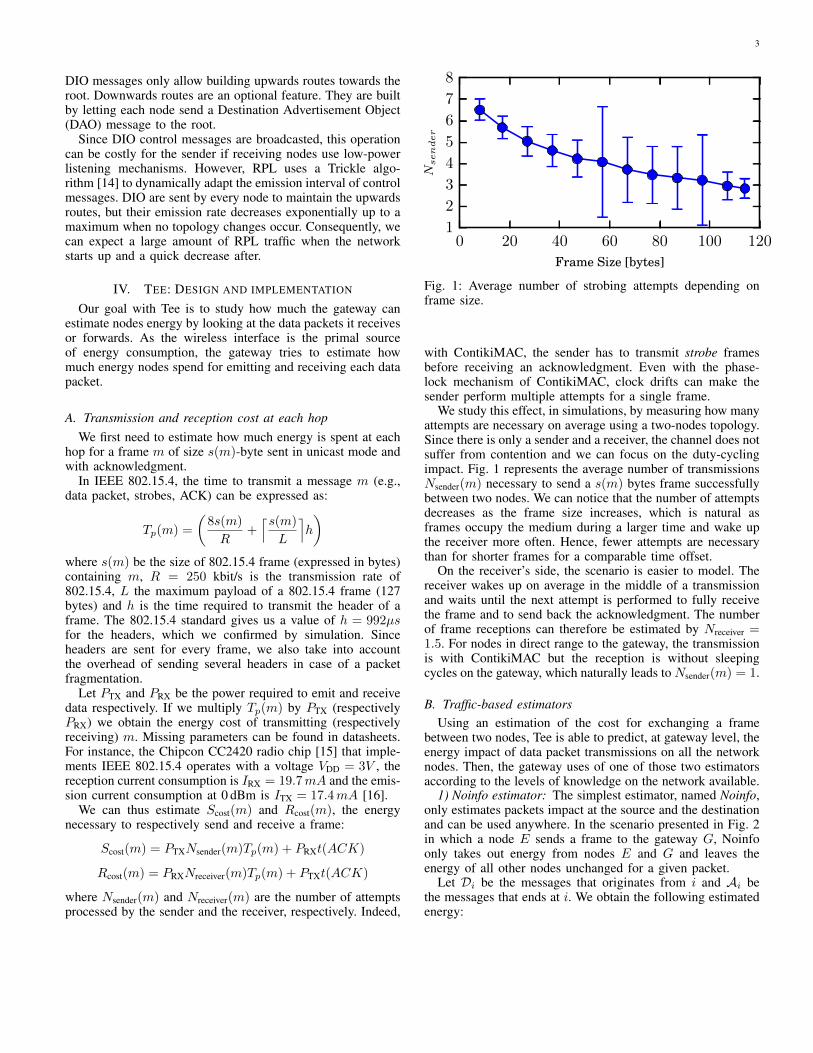
Fig. 1: Average number of strobing attempts depending onframe size.

with ContikiMAC, the sender has to transmit strobe framesbefore receiving an acknowledgment. Even with the phase-lock mechanism of ContikiMAC, clock drifts can make thesender perform multiple attempts for a single frame.

We study this effect, in simulations, by measuring how manyattempts are necessary on average using a two-nodes topology.Since there is only a sender and a receiver, the channel does notsuffer from contention and we can focus on the duty-cyclingimpact. Fig. 1 represents the average number of transmissionsNsender(m) necessary to send a s(m) bytes frame successfullybetween two nodes. We can notice that the number of attemptsdecreases as the frame size increases, which is natural asframes occupy the medium during a larger time and wake upthe receiver more often. Hence, fewer attempts are necessarythan for shorter frames for a comparable time offset.

On the receiver’s side, the scenario is easier to model. Thereceiver wakes up on average in the middle of a transmissionand waits until the next attempt is performed to fully receivethe frame and to send back the acknowledgment. The numberof frame receptions can therefore be estimated by Nreceiver =1.5. For nodes in direct range to the gateway, the transmissionis with ContikiMAC but the reception is without sleepingcycles on the gateway, which naturally leads to Nsender(m) = 1.

B. Traffic-based estimatorsUsing an estimation of the cost for exchanging a frame

between two nodes, Tee is able to predict, at gateway level, theenergy impact of data packet transmissions on all the networknodes. Then, the gateway uses of one of those two estimatorsaccording to the levels of knowledge on the network available.

1) Noinfo estimator: The simplest estimator, named Noinfo,only estimates packets impact at the source and the destinationand can be used anywhere. In the scenario presented in Fig. 2in which a node E sends a frame to the gateway G, Noinfoonly takes out energy from nodes E and G and leaves theenergy of all other nodes unchanged for a given packet.

Let Di be the messages that originates from i and Ai bethe messages that ends at i. We obtain the following estimatedenergy:

4

G

E

routers (receive and emit)

overhearers (receive)

neutral

Fig. 2: Nodes potentially impacted by the forwarding of aframe from node E to gateway G.

Ei(t) =∑

m∈Di(t)

Scost(m) +∑

m∈Ai(t)

Rcost(m).

This estimator requires no knowledge and under-estimatesthe effect of a packet on the network unless all nodes arein-range of the gateway. For instance, it does not capturetransmissions induced by forwarding actions at intermediarynodes.

2) Route estimator: In multi-hop topologies, the gatewaywill likely be aware of the network active routes by usingnetwork mapping tools or through the routing protocol.

The second estimator we examine, referred to as Route, usesthis information and subtracts from the remaining energy ofeach node on the route (dark gray nodes in Fig. 2) the cost ofa reception and an emission of the frame.

Let Fi be the message set forwarded by the node i whileit’s neither the destination nor the source of the message.

Ei(t) =∑

m∈Di(t)∪Fi(t)

Scost(m) +∑

m∈Ai(t)∪Fi(t)

Rcost(m)

V. EXPERIMENTAL RESULTS

We evaluated the accuracy of the different estimators de-scribed above using the COOJA simulator with its Power-tracker extension, which measures and reports the time spentby each node in reception and transmission state with 1µsresolution. All nodes run the latest development branch ofContiki and use RPL for routing and ContikiMAC over IEEE802.15.4.

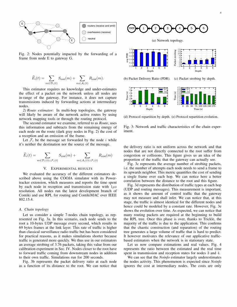
A. Chain topologyLet us consider a simple 7-nodes chain topology, as rep-

resented on Fig. 3a. In this scenario, each node sends to theroot a 10-bytes UDP message every second, which results in69 bytes frames at the link layer. This rate of traffic is higherthan classical surveillance radio traffic but has been consideredfor practical reasons, as it makes simulations shorter becausetraffic is generated more quickly. We thus use in our estimatorsan average strobing of 3.76 packets, taking this value from ourcalibration experiment in Sec. IV. Nodes closer to the root haveto forward traffic coming from downstream nodes in additionto their own traffic. Simulations run for 200 seconds.

Fig. 3b represents the packet delivery ratio at each nodeas a function of its distance to the root. We can notice that

(a) Network topology.

1 2 3 4 5 6Depth

0.0

0.2

0.4

0.6

0.8

1.0

avg

PD

R

(b) Packet Delivery Ratio (PDR).

1 2 3 4 5 6Depth

−202468

101214

Pack

etst

robi

ng

(c) Packet strobing by depth.

1 2 3 4 5 6Depth

0123456

Tim

e[s

]

rpludp

(d) Protocol repartition by depth.

0 25 50 75 100 125 150 175Time [s]

0.00.51.01.52.02.53.03.54.04.5

Tim

e[s

]

rpludp

(e) Protocol repartition evolution.

Fig. 3: Network and traffic characteristics of the chain exper-iment.

the delivery ratio is not uniform across the network and thatnodes that are not directly connected to the root suffer fromcongestion or collisions. This figure gives us an idea of theproportion of the traffic that the gateway can actually see.

Fig. 3c represents the average number of strobing packets,i.e. the number of attempts each node needs to send a frame toits upwards neighbor. This metric quantifies the cost of sendinga single frame over each hop. We can notice here a bettercorrelation between the distance to the root and this figure.

Fig. 3d represents the distribution of traffic types at each hop(UDP and routing messages). This measurement is important,as it shows the amount of control traffic that the gatewaymay not measure and shall infer. We can notice that, at thisstage, the traffic is almost identical for the different nodes andhence could be modeled by a constant rate. However, Fig. 3eshows the evolution over time. As expected, we can notice thatmany routing packets are required at the beginning to buildthe RPL tree. Once this phase is over, thanks to Trickle, themajority of the traffic is due to the application. This confirmsthat the chaotic construction (and reparation) of the routingtree generates a large volume of traffic that is hard to predict.It however motivates the relevance of our applicative traffic-based estimators when the network is in stationary state.

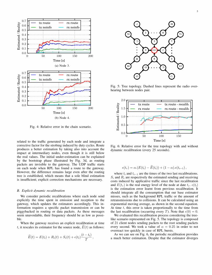
Let us now compare estimations and real values. Fig. 4represents the ratio between the estimated and the real timespent in transmission and reception states for nodes 3 and 4.

We can see that the Noinfo estimator largely underestimatesthe nodes activity. This phenomenon is expected since Noinfoignores the cost at intermediary nodes. The costs are only

5

0 50 100 150 200

Time [s]

0.0

0.1

0.2

0.3

0.4

0.5

0.6

0.7E

stim

ated

/Rea

lity tx route

tx noinforx routerx noinfo

(a) Node 3.

50 100 150 200

Time [s]

0.0

0.1

0.2

0.3

0.4

0.5

0.6

0.7

Est

imat

ed/R

ealit

y tx routetx noinfo

rx routerx noinfo

(b) Node 4.

Fig. 4: Relative error in the chain scenario.

related to the traffic generated by each node and integrate acorrective factor for the strobing induced by duty cycles. Routeproduces a better estimation by taking also into account theimpact at intermediary nodes, even though it is still belowthe real values. The initial under-estimation can be explainedby the bootstrap phase illustrated by Fig. 3d, as routingpackets are invisible to the gateway. The UDP traffic startson each node when RPL has found a route to the gateway.However, the difference remains large even after the routingtree is established, which means that a sole blind estimationis insufficient; explicit correction mechanisms are necessary.

B. Explicit dynamic recalibration

We consider periodic recalibrations where each node sendexplicitly the time spent in emission and reception to thegateway, which updates the estimators accordingly. This in-formation requires a specific packet transmission or can bepiggybacked in routing or data packets. As these messagesseem unavoidable, their frequency should be as low as possi-ble.

When the gateway receives an explicit recalibration at timet, it rescales its estimator for the source node, E(t) as follows:

E(t) = E(tr) +Ri(t) + Si(t) + ε(tr)(t− tr)T

,

Fig. 5: Tree topology. Dashed lines represent the radio over-hearing between nodes pair.

0 50 100 150

Time [s]

0.0

0.5

1.0

1.5

2.0

Est

imat

ed/R

ealit

y tx routerx route

tx route - recalib.rx route - recalib.

Fig. 6: Relative error for the tree topology with and withoutdynamic recalibration (every 25 seconds).

ε(tr) = α.(E(tr)− E(tr)) + (1− α).ε(tr−1) ,where tr and tr−1 are the times of the two last recalibrations.

Si and Ri are respectively the estimated sending and receivingcosts induced by applicative traffic since the last recalibrationand E(tr) is the real energy level of the node at date tr. ε(tr)is the estimation error learnt from previous recalibration. Itshould integrate all the consumption that our base estimatormisses, such as the background RPL traffic or the amount ofretransmissions due to collisions. It can be calculated using anexponential moving average, as shown in the second equation.At time t, this error is taken proportionally to the time fromthe last recalibration (occurring every T ). Note that ε(0) = 0.

We evaluated this recalibration process considering the tree-like scenario represented on Fig. 5. The topology is composedof 21 client nodes sending packets to the root sending packetsevery second. We took a value of α = 0.25 in order to notoverreact too quickly in case of RPL bursts.

As we can see on Fig. 6, the periodic recalibration providesa much better estimation. Despite that the estimator diverges

6

10 25 50 75 100Calibration Interval [s]

0.0

0.2

0.4

0.6

0.8

1.0

Est

imat

ion

/Rea

lity

Fig. 7: Average relative error for different recalibration inter-vals.

at the beginning, due to network bootstrap as explained inSec. V-A, it quickly provides accurate predictions of the en-ergy depletion. When the recalibration happens, the estimatorintegrates the average error from previous recalibrations andconverge quickly to accurate estimation.

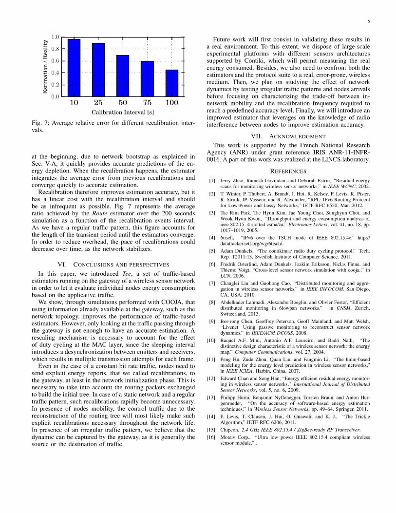
Recalibration therefore improves estimation accuracy, but ithas a linear cost with the recalibration interval and shouldbe as infrequent as possible. Fig. 7 represents the averageratio achieved by the Route estimator over the 200 secondssimulation as a function of the recalibration events interval.As we have a regular traffic pattern, this figure accounts forthe length of the transient period until the estimators converge.In order to reduce overhead, the pace of recalibrations coulddecrease over time, as the network stabilizes.

VI. CONCLUSIONS AND PERSPECTIVES

In this paper, we introduced Tee, a set of traffic-basedestimators running on the gateway of a wireless sensor networkin order to let it evaluate individual nodes energy consumptionbased on the applicative traffic.

We show, through simulations performed with COOJA, thatusing information already available at the gateway, such as thenetwork topology, improves the performance of traffic-basedestimators. However, only looking at the traffic passing throughthe gateway is not enough to have an accurate estimation. Arescaling mechanism is necessary to account for the effectof duty cycling at the MAC layer, since the sleeping intervalintroduces a desynchronization between emitters and receivers,which results in multiple transmission attempts for each frame.

Even in the case of a constant bit rate traffic, nodes need tosend explicit energy reports, that we called recalibrations, tothe gateway, at least in the network initialization phase. This isnecessary to take into account the routing packets exchangedto build the initial tree. In case of a static network and a regulartraffic pattern, such recalibrations rapidly become unnecessary.In presence of nodes mobility, the control traffic due to thereconstruction of the routing tree will most likely make suchexplicit recalibrations necessary throughout the network life.In presence of an irregular traffic pattern, we believe that thedynamic can be captured by the gateway, as it is generally thesource or the destination of traffic.

Future work will first consist in validating these results ina real environment. To this extent, we dispose of large-scaleexperimental platforms with different sensors architecturessupported by Contiki, which will permit measuring the realenergy consumed. Besides, we also need to confront both theestimators and the protocol suite to a real, error-prone, wirelessmedium. Then, we plan on studying the effect of networkdynamics by testing irregular traffic patterns and nodes arrivalsbefore focusing on characterizing the trade-off between in-network mobility and the recalibration frequency required toreach a predefined accuracy level. Finally, we will introduce animproved estimator that leverages on the knowledge of radiointerference between nodes to improve estimation accuracy.

VII. ACKNOWLEDGMENT

This work is supported by the French National ResearchAgency (ANR) under grant reference IRIS ANR-11-INFR-0016. A part of this work was realized at the LINCS laboratory.

REFERENCES

[1] Jerry Zhao, Ramesh Govindan, and Deborah Estrin, “Residual energyscans for monitoring wireless sensor networks,” in IEEE WCNC, 2002.

[2] T. Winter, P. Thubert, A. Brandt, J. Hui, R. Kelsey, P. Levis, K. Pister,R. Struik, JP. Vasseur, and R. Alexander, “RPL: IPv6 Routing Protocolfor Low-Power and Lossy Networks,” IETF RFC 6550, Mar. 2012.

[3] Tae Rim Park, Tae Hyun Kim, Jae Young Choi, Sunghyun Choi, andWook Hyun Kwon, “Throughput and energy consumption analysis ofieee 802.15. 4 slotted csma/ca,” Electronics Letters, vol. 41, no. 18, pp.1017–1019, 2005.

[4] 6tisch, “IPv6 over the TSCH mode of IEEE 802.15.4e,” http://datatracker.ietf.org/wg/6tisch/.

[5] Adam Dunkels, “The contikimac radio duty cycling protocol,” Tech.Rep. T2011:13, Swedish Institute of Computer Science, 2011.

[6] Fredrik Österlind, Adam Dunkels, Joakim Eriksson, Niclas Finne, andThiemo Voigt, “Cross-level sensor network simulation with cooja.,” inLCN, 2006.

[7] Changlei Liu and Guohong Cao, “Distributed monitoring and aggre-gation in wireless sensor networks,” in IEEE INFOCOM, San Diego,CA, USA, 2010.

[8] Abdelkader Lahmadi, Alexandre Boeglin, and Olivier Festor, “Efficientdistributed monitoring in 6lowpan networks,” in CNSM, Zurich,Switzerland, 2013.

[9] Bor-rong Chen, Geoffrey Peterson, Geoff Mainland, and Matt Welsh,“Livenet: Using passive monitoring to reconstruct sensor networkdynamics,” in IEEE/ACM DCOSS, 2008.

[10] Raquel A.F. Mini, Antonio A.F. Loureiro, and Badri Nath, “Thedistinctive design characteristic of a wireless sensor network: the energymap,” Computer Communications, vol. 27, 2004.

[11] Peng Hu, Zude Zhou, Quan Liu, and Fangmin Li, “The hmm-basedmodeling for the energy level prediction in wireless sensor networks,”in IEEE ICIEA, Harbin, China, 2007.

[12] Edward Chan and Song Han, “Energy efficient residual energy monitor-ing in wireless sensor networks,” International Journal of DistributedSensor Networks, vol. 5, no. 6, 2009.

[13] Philipp Hurni, Benjamin Nyffenegger, Torsten Braun, and Anton Her-genroeder, “On the accuracy of software-based energy estimationtechniques,” in Wireless Sensor Networks, pp. 49–64. Springer, 2011.

[14] P. Levis, T. Clausen, J. Hui, O. Gnawali, and K. J., “The TrickleAlgorithm,” IETF RFC 6206, 2011.

[15] Chipcon, 2.4 GHz IEEE 802.15.4 / ZigBee-ready RF Transceiver.[16] Moteiv Corp., “Ultra low power IEEE 802.15.4 compliant wireless

sensor module,” .