TECHNOLOGYâ€“CLIMATE INTERACTIONS IN THE GREEN REVOLUTION IN INDIA

ECONOMIC GROWTH CENTER

YALE UNIVERSITY

P.O. Box 208269New Haven, Connecticut 06520-8269

CENTER DISCUSSION PAPER NO.805

TECHNOLOGY–CLIMATE INTERACTIONS IN THEGREEN REVOLUTION IN INDIA

James W. McKinsey, Jr.Bryant College

Robert E. EvensonYale University

August 1999

Note: Center Discussion Papers are preliminary materials circulated to stimulate discussions and criticalcomments.

* This paper is based on McKinsey's unpublished 1998 Yale Ph.D. dissertation HYV's,Multiple-Cropping, Irrigation, Climate and the Green Revolution in India, written under thedirection of Prof. Evenson. The assistance of Bruce Dixon, Robert Mendelsohn, ArielDinar and three anonymous referees is gratefully acknowledged; all usual disclaimersapply

TECHNOLOGY–CLIMATE INTERACTIONSIN THE GREEN REVOLUTION IN INDIA*

James W. McKinsey, Jr.

Robert E. Evenson

Abstract

This paper presents a model of the Green Revolution in India, in which the development and diffusion ofHYVs, the expansion of irrigation and the expansion of multiple-cropping are treated as endogenousresponses to more basic investments in agricultural technology and infrastructure, as well as to climateand edaphic endowments. We incorporate explicit climate-technology interactions in the model, inorder to identify climate effects on the diffusion of HYVs, irrigation and multiple-cropping, and on NetRevenue to agriculture. We find that climate affects technology development and diffusion, and thattechnology development and diffusion affect the impacts of climate on agricultural productivity in India.

Key words: Green Revolution, India, HYV, Rice, Wheat, Climate, Agricultural Research

JEL classifications: 112, 121, 226, 620, 710

McKinsey: Department of Economics, Bryant College, Douglas Pike, Smithfield, [email protected]

Evenson: Economic GrowthCenter, Yale University, Box 208269, New Haven,CT, 06520 [email protected]

TECHNOLOGY–CLIMATE INTERACTIONSIN THE GREEN REVOLUTION IN INDIA

James W. McKinsey, Jr.Bryant College

Robert E. EvensonYale University

I. INTRODUCTION

During the past thirty years significant portions of India’s agriculture have undergone a transformation

known as the Green Revolution, which can largely be characterized by three processes: the

development and diffusion of new, high-yielding varieties [HYV] of food crops1, the expansion of

(especially tube-well) irrigation, and the expansion of multiple-cropping.

A number of studies of the productivity growth in Indian agriculture associated with the Green

Revolution have been completed. Most prior studies have treated the three main components of the

Green Revolution as exogenous variables in district-level empirical analyses (Evenson and McKinsey

[1991]; Evenson, Rosegrant and Pray [1999]). In spite of the importance to agricultural production of

land, water and sunlight, the prior studies included no edaphic or climate variables beyond area planted

and current rainfall.

Alternative models have been developed during the past decade, explicitly including edaphic and

climate variables, which are designed to explain land values or farm profits. Called Ricardian models,

they were first applied to US agriculture by Mendelsohn, Nordhaus and Shaw [1993; 1994], and more

recently in essentially the same form to agriculture in India by Kumar and Parkikh [1998] and by

Sanghi, Mendelsohn and Dinar [1998]. These latter two studies have taken some features of

agricultural technology into account but have not developed a full treatment of the technology dimension

in Indian agriculture.

1 Primarily rice and wheat, but to a lesser extent maize and some minor food crops.

* This paper is based on McKinsey's unpublished 1998 Yale Ph.D. dissertation HYV's,Multiple-Cropping, Irrigation, Climate and the Green Revolution in India, written under thedirection of Prof. Evenson. The assistance of Bruce Dixon, Robert Mendelsohn, ArielDinar and three anonymous referees is gratefully acknowledged; all usual disclaimersapply

McKinsey [1998] has developed a model of Indian agriculture which treats the three components of

the Green Revolution as endogenous responses to more basic investments in agricultural technology and

infrastructure. We extend the Ricardian idea into McKinsey’s technology model, and incorporate

explicit climate-technology interactions, in order to identify climate effects on the diffusion of HYVs,

irrigation and multiple-cropping, and on Net Revenue to agriculture. We thus investigate whether

district-level climate differences conditioned the regional pattern of investment and technology adoption

as the Green Revolution unfolded, and conversely whether the processes of change which constitute the

Green Revolution might modify or ameliorate the effects of future climate change. We recognize the

difficulty inherent in trying to predict future climate change, let alone future technological change; but we

expect some continuity in the processes underlying these three technological developments and thus use

current cross-section differences in climate and technology as proxies for future time-series changes in

both sets of variables.

Part II of the paper reviews the methodology underlying the specifications. Part III reports estimates

of the four equations in our model which capture the processes of the Green Revolution and Net

Revenue to crop production. Based on these estimates Parts IV and V report the climate sensitivity of

(that is, the impact of differences or changes in climate on) technological change and of Net Revenue,

and the effects of technological change on the climate sensitivity of Net Revenue.

II. METHODOLOGY

A. The Model

In this paper we capture the technical core of the Green Revolution in three simultaneous equations,

estimated by 2SLS. The endogenous variables measure the processes described above: the

Technology-Climate Interactions and the Green Revolution in India McKinsey & Evenson page 2

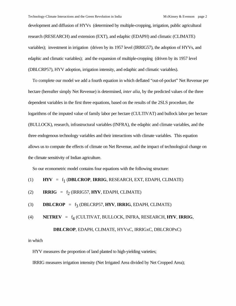
development and diffusion of HYVs (determined by multiple-cropping, irrigation, public agricultural

research (RESEARCH) and extension (EXT), and edaphic (EDAPH) and climatic (CLIMATE)

variables); investment in irrigation (driven by its 1957 level (IRRIG57), the adoption of HYVs, and

edaphic and climatic variables); and the expansion of multiple-cropping (driven by its 1957 level

(DBLCRP57), HYV adoption, irrigation intensity, and edaphic and climatic variables).

To complete our model we add a fourth equation in which deflated “out-of-pocket” Net Revenue per

hectare (hereafter simply Net Revenue) is determined, inter alia, by the predicted values of the three

dependent variables in the first three equations, based on the results of the 2SLS procedure, the

logarithms of the imputed value of family labor per hectare (CULTIVAT) and bullock labor per hectare

(BULLOCK), research, infrastructural variables (INFRA), the edaphic and climate variables, and the

three endogenous technology variables and their interactions with climate variables. This equation

allows us to compute the effects of climate on Net Revenue, and the impact of technological change on

the climate sensitivity of Indian agriculture.

So our econometric model contains four equations with the following structure:

(1) HYV = f1 (DBLCROP, IRRIG, RESEARCH, EXT, EDAPH, CLIMATE)

(2) IRRIG = f2 (IRRIG57, HYV, EDAPH, CLIMATE)

(3) DBLCROP = f3 (DBLCRP57, HYV, IRRIG, EDAPH, CLIMATE)

(4) NETREV = f4 (CULTIVAT, BULLOCK, INFRA, RESEARCH, HYV, IRRIG,

DBLCROP, EDAPH, CLIMATE, HYVxC, IRRIGxC, DBLCROPxC)

in which

HYV measures the proportion of land planted to high-yielding varieties;

IRRIG measures irrigation intensity (Net Irrigated Area divided by Net Cropped Area);


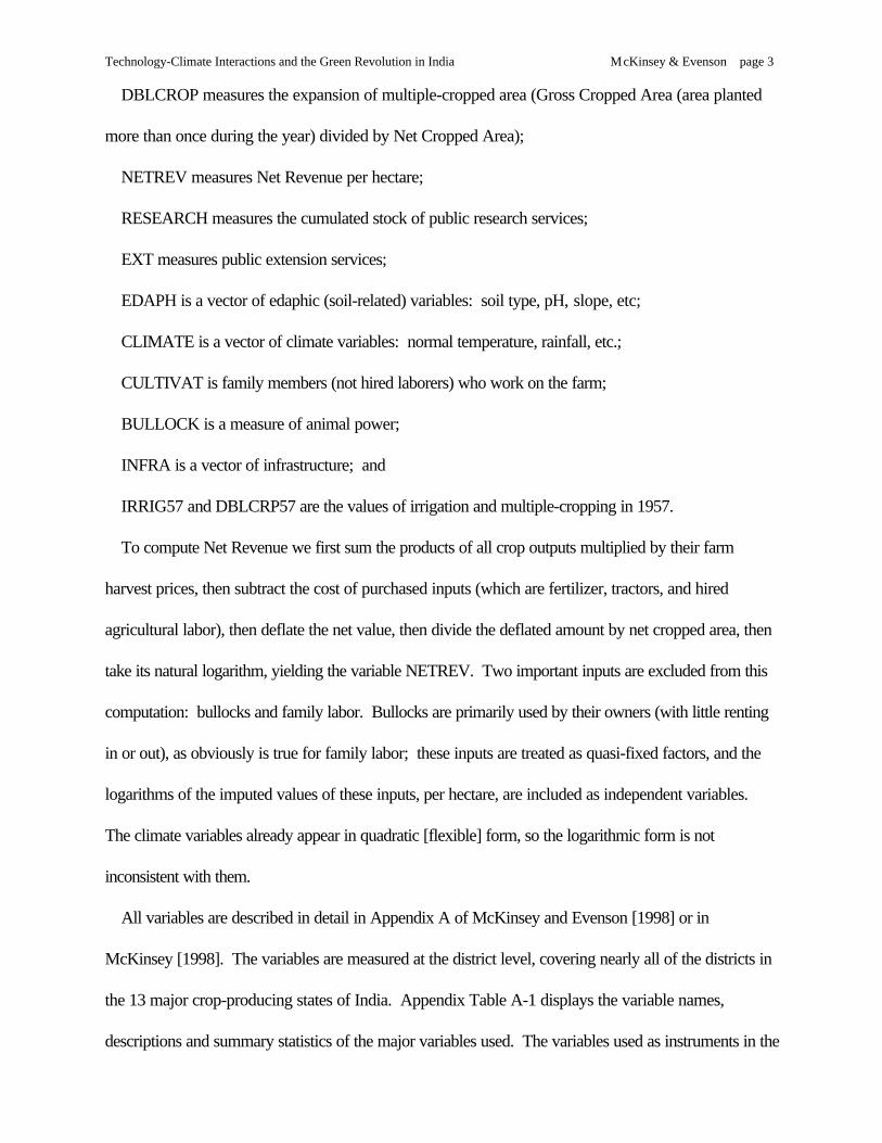
DBLCROP measures the expansion of multiple-cropped area (Gross Cropped Area (area planted

more than once during the year) divided by Net Cropped Area);

NETREV measures Net Revenue per hectare;

RESEARCH measures the cumulated stock of public research services;

EXT measures public extension services;

EDAPH is a vector of edaphic (soil-related) variables: soil type, pH, slope, etc;

CLIMATE is a vector of climate variables: normal temperature, rainfall, etc.;

CULTIVAT is family members (not hired laborers) who work on the farm;

BULLOCK is a measure of animal power;

INFRA is a vector of infrastructure; and

IRRIG57 and DBLCRP57 are the values of irrigation and multiple-cropping in 1957.

To compute Net Revenue we first sum the products of all crop outputs multiplied by their farm

harvest prices, then subtract the cost of purchased inputs (which are fertilizer, tractors, and hired

agricultural labor), then deflate the net value, then divide the deflated amount by net cropped area, then

take its natural logarithm, yielding the variable NETREV. Two important inputs are excluded from this

computation: bullocks and family labor. Bullocks are primarily used by their owners (with little renting

in or out), as obviously is true for family labor; these inputs are treated as quasi-fixed factors, and the

logarithms of the imputed values of these inputs, per hectare, are included as independent variables.

The climate variables already appear in quadratic [flexible] form, so the logarithmic form is not

inconsistent with them.

All variables are described in detail in Appendix A of McKinsey and Evenson [1998] or in

McKinsey [1998]. The variables are measured at the district level, covering nearly all of the districts in

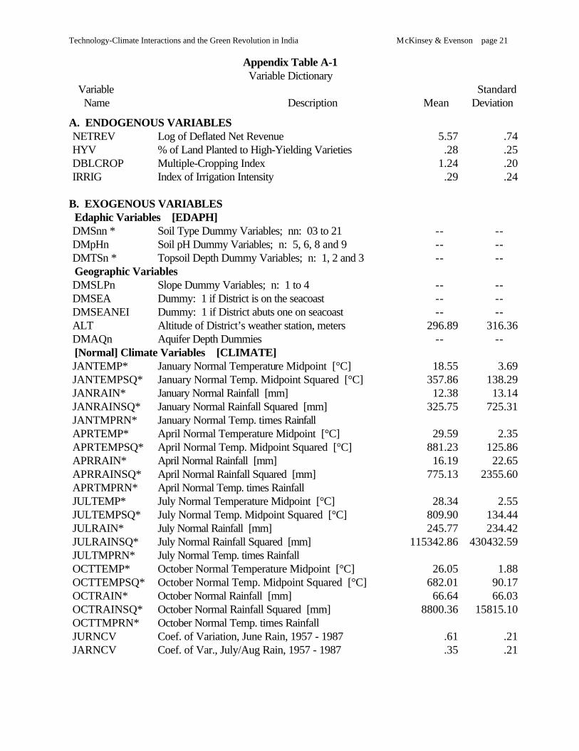
the 13 major crop-producing states of India. Appendix Table A-1 displays the variable names,

descriptions and summary statistics of the major variables used. The variables used as instruments in the


2SLS system are denoted in Appendix Table A-1 by an asterisk following the variable name. These

instruments include fundamental climatic and edaphic variables, as well as two technology variables and

a number of price ratios proxying institutional factors.

The climate variables are computed from 30-year averages recorded at various Climatological

Observatories and Rainguage Stations by the Indian Meteorological Department, usually using data

between 1931 and 1960. These variables represent long-term norms, to which farmers have

responded in their decisions about cropping patterns, input use, investment in technology and

infrastructure, and so forth. These climate norms obviously vary only across districts, with no time-

series variation.

This study applies to the years 1970/71 through 1987/88. By 1970 the use of modern high-yielding

varieties of several crops had become established in nearly every district, and partly in concert with the

expansion of HYV there was substantial new investment in irrigation, fertilizer distribution, research and

extension activities, and so forth.

B. Adaptation and Interaction

Expressions such as (1) through (4) allow for farmer adaptation to regional climate conditions (and to

changes in climate which might occur over long periods of time into the future). This adaptation includes

investments in farm level irrigation and drainage as well as changes in farm practices including cropping

patterns. There is, as well, potential adaptation by the organizations producing technology and

infrastructure for farmers. These organizations include private firms which conduct R&D to develop

improved factors to be supplied to the agricultural sector, and the public sector agricultural research and

extension organizations which also provide improved technology to agriculture. It also includes public

sector units providing, and maintaining, infrastructure.

Implicitly, this suggests that there may be important climate-technology and climate-infrastructure

interactions. These interactions enable us to estimate two dimensions of the technology–climate


relationship. In the system (1) through (3) we estimate the effects of (current regional differences in)

climate [C] on the production and diffusion of technology [T]. (That is, we can compute dT/dC.) From

these estimates we can ask: How might an increase in normal temperatures and rainfall affect the

development and diffusion of agricultural technology? From the estimation of (4) with interaction terms

we can ask the following question: What might be the impact of an increase in rainfall and temperature

on Net Revenue [NR] (including the effects operating through technology)?

(5) dNR/dC = ∂NR/∂C + ∂NR/∂T • dT/dC

We can also capture two sets of secondary impacts. The first is the impact of technology on the

climate effects:

(6) d(dNR/dC)/dT

which enables us to ask whether the climate sensitivity of Net Revenue per hectare was influenced by

changes in the technology variables during the period of the Green Revolution, indicating whether this

process of technological change might continue to benefit Indian agriculture in the context of projected

warming in the future. The second set of secondary impacts is the impact of climate change on the

technology effects:

(7) d(dNR/dT)/dC

(which of course is equal to equation (6)), indicating what impact future climate change might have on

the benefits which the processes of technical change have conferred on Indian agriculture.

III. ESTIMATION

The models described thus far impose no restrictions on the functional form to be estimated. We use

a very general form, with quadratic and interaction terms in order to capture non-linearities and

moderating impacts of technology on climate effects and vice versa. The modern varieties, multiple-

cropping and irrigation intensity equations are estimated in the 2SLS system with linear and

quadratic terms for climate variables.


Obvious econometric issues in this study involve the existence of heteroscedasticity, multicollinearity,

and specification issues of variable inclusion or exclusion.

The Net Revenue equation is weighted by net cropped area, to adjust for heteroscedasticity.

Standard errors have been estimated by White’s consistent estimator of the least squares covariance

matrix, and the resultant estimated t-ratios are consistent.

The problems of multicollinearity are likely to be severe, given the inclusion of so many climate terms,

and their squares. Their inclusion is crucial and the squared terms are necessary to allow for

nonlinearities in climate effects. One should use caution in interpreting or using any individual

coefficient estimate: its true value may substantially differ from its estimated value, and the variable may

be a valid, important regressor even if the estimated t-ratio is below the customary critical value. But

the computations of estimated effects of climate change, using all the estimated coefficients, are likely to

be valid, for any mis-estimation of the value of one coefficient is likely to be compensated for in the

estimation of the values of the coefficients of the other collinear variables; thus the joint impact of all the

variables together is probably much more accurate (Segerson & Dixon, [1996]).

In the Ricardian estimates of Mendelsohn et al., [1994] a cross-section of land values was regressed

on climate (CLIMATE), edaphic (EDAPH) and infrastructure (I) variables. Prices and technology

variables were excluded on the grounds either that prices did not vary in their single-year cross-section

for specific commodities or that transport-related differentials would continue in the future, and that

technology was “equally” accessible to all farmers in the United States; obviously this precluded

climate-technology interaction estimates. In the analysis reported here, multiple years are compared so

that prices do vary across the sample and must be included.

Furthermore, a large number of agricultural productivity studies have measured significant differences

in cross-section productivity levels which are at least partly due to edaphic and climate differences.

More importantly, the studies have also measured time series differences in rate of change of partial or


total factor productivity change for different regions (Huffman & Evenson [1993] (U.S.), Avila &

Evenson [1995] (Brazil), Evenson & McKinsey [1991] (India)). These differences have persisted over

long periods of time and have been related to cross-section [and time-series] differences in investments

in regionally oriented agricultural research programs.

One might argue (as Mendelsohn et al. [1994] do in the context of the United States) that regional

differences in productivity growth are likely to “converge” over time as technology from the leading

regions is diffused to the laggard regions. If so, the regional productivity differences would not be

capitalized into land values. Yet this is quite unlikely in India, given the nature of agricultural technology

which is highly location-specific. Studies of agricultural research (again, Evenson & McKinsey [1991];

Evenson, Rosegrant & Pray [1999]) indicate that regions with little or no research effort targeted to

their particular climate and edaphic conditions remain laggard regions. And even if productivity were to

converge over time, current Net Revenues would still reflect existing productivity differences.

Similarly, variables measuring current weather are important in Net Revenue specifications, but not in

land value specifications where current weather gets averaged into climate.

IV. ESTIMATES

A. Technology

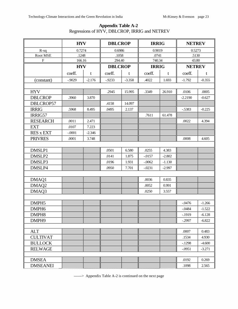
The first four columns of Appendix Table A-2 display the results from the second stage regression on

HYV, DBLCROP, and IRRIG. A number of striking results emerge. First is the degree to which this

system captures the modeled behavior. Grossly, all three second-stage regressions have highly

significant F-statistics and high R-squareds, with low Root MSE. Even more important than the general

goodness-of-fit of these regression equations, and the significance of groups of variables, are the

patterns revealed within each equation.


Slope significantly influences multiple-cropping. Irrigation intensity tends to be higher in the flattest

districts, and in districts above aquifers which are geologically thickest2. The adoption of modern high-

yielding varieties, multiple-cropping and irrigation are mutually-reinforcing: the coefficients of both

DBLCROP and IRRIG on HYV are significantly positive, as are the coefficients of both HYV and

IRRIG on DBLCROP and the coefficient of HYV on IRRIG. (See Section V.A below.)

The adoption of modern varieties also responds favorably to greater extension activity and to higher

public and private research. Public research and extension are substitutes in determining HYV

adoption.

There is considerable inertia in this behavior: both the extent of multiple-cropping and irrigation

intensity are highest in those districts in which such activity had been largest in 1957.

B. Net Revenue

The first and last columns of Appendix Table A-2 display the results of the regression of Net

Revenue on edaphic, climatic, and geographic variables, the predicted values of the technology and

infrastructure variables from the two-stage system described above, interactions between climate and

technology or between climate and infrastructure, and dummy variables for time. This equation also fits

the data well: the R2 is above 0.5, and the F-statistic is highly significant although perhaps the fit is not

quite as good as it is in the three technology equations.

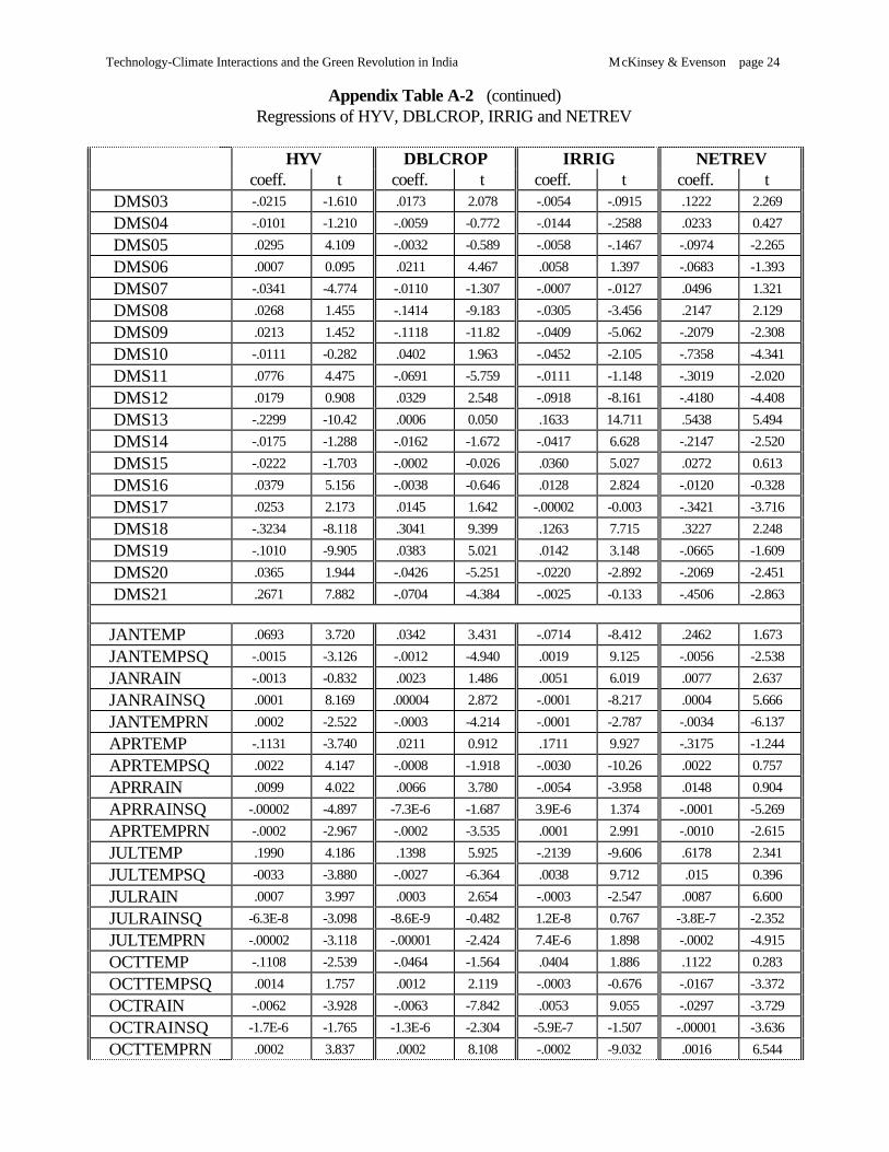
The edaphic variables are important determinants of Net Revenue: thirteen of the nineteen soil type

dummies have significant coefficients, and alkali soil (pH of eight, nine or higher) reduces Net Revenue.

While the coefficients on the predicted values of modern varieties [HYV_P], multiple-cropping

[DBLCRP_P], and irrigation intensity [IRRIG_P] are not significantly different from zero, those

variables are interacted with climate terms, as discussed below, and more than half of the interactions’

2 This does not measure the annual water depth within the aquifer, but rather a long term geological potential.Farmers may respond to this in their cropping choices; farmers and probably governments also respond in theirirrigation investments.


coefficients are significant, two-thirds of them positive. Research contributes significantly to Net

Revenue.

Net Revenue is lower in districts with relatively more bullocks, perhaps reflecting the use of an older

(and less profitable) package of inputs and practices in those districts. An increase in the ratio of off-

farm wages relative to agricultural wages reduces Net Revenue, which may denote a decline in the

quality of available farm workers, or even a reduction in the amount of time devoted to agriculture by

owner-cultivators, as off-farm opportunities attract more and more of the best and most-highly-skilled

laborers. Current weather, and its timing, also obviously influences current Net Revenue: given a

normal seasonal rainfall, higher rainfall in July and August (the variable JUAURAIN) will increase Net

Revenue3. Interestingly a higher coefficient of variation of rainfall contributes to Net Revenue4. This

model displays quite rich (normal) temperature and rainfall effects on Net Revenue. The squared and

“raw” terms are usually of the opposite sign. The impacts of temperature and rainfall differ by month.

A key focus of this study is the interaction of climate with technology, infrastructure, and geographic

variables, beyond the so-called “purely climate” variables. Six such interactions each month are

included. The interactions of normal temperature and rainfall with the predicted values of modern

varieties, multiple-cropping and irrigation intensity are complex, yielding fourteen significant coefficients

out of twenty-four, nine of them positive. Higher HYV adoption tends to increase Net Revenue in

districts with higher July temperature and rainfall, but to be associated with lower Net Revenue in

districts with higher January rainfall (which are likely to be districts in which irrigated winter wheat is not

grown) and with higher April temperatures. Higher cropping intensity tends to increase Net Revenue in

districts with higher April rainfall and with higher October temperature and rainfall (which, in most areas

3 Probably occurring during crucial maturation phases of many important crops in most states; actual June rain[holding constant the level of normal seasonal rainfall] had a negative but insignificant coefficient, perhaps reflectingthe difficulty in planting when the ground is too wet.4 This may reflect monsoon timing: a higher coefficient of variation may indicate that the rains were spread moreevenly across the monsoon season.


of India, is a month when the “second” crop is growing), but is associated with lower Net Revenue in

districts with higher July temperature and rainfall (which, in many areas of India, is a month when the

primary crop is growing). And higher irrigation intensity tends to increase Net Revenue in districts with

higher January, April and July temperatures as well as higher April rainfall, but is associated with lower

Net Revenue in districts with higher October temperature.

V. INTERPRETATION OF RESULTS

A. Technological Change Relationships

The first three equations in our model describe the technology components of the Green Revolution

experience in India. Recall that we model the adoption of modern varieties as a function, inter alia, of

investment in irrigation and the spread of multiple-cropping; we model the spread of multiple-cropping

as a function, inter alia, of the adoption of modern varieties and investment in irrigation infrastructure;

and we model the spread of irrigation as a function, inter alia, of the adoption of modern varieties.

From the estimated coefficients in those three equations we can compute the impact of an increase in

any of the technology variables on the adoption or spread of the other two. Those effects are presented

in Table 1 in elasticity form, showing the proportional change in the variable in the columns in response

to a one percent increase in the variables in the rows. For example, the second entry in the HYV

column indicates that a one percent increase in multiple-cropping would induce approximately two-fifths

of one percent increase in the adoption of modern varieties.

It is clear from Table 1 that the increased adoption of modern varieties has been an important spur to

the investment in irrigation facilities and to the expansion of multiple-cropping (the top row of estimates)

at the same time that the adoption of the modern varieties themselves have responded strongly to the

expansion of irrigation and multiple-cropping (the left column of estimates). The effects of multiple-

cropping and irrigation on each other, while positive, have been less pronounced. Taken as a whole,


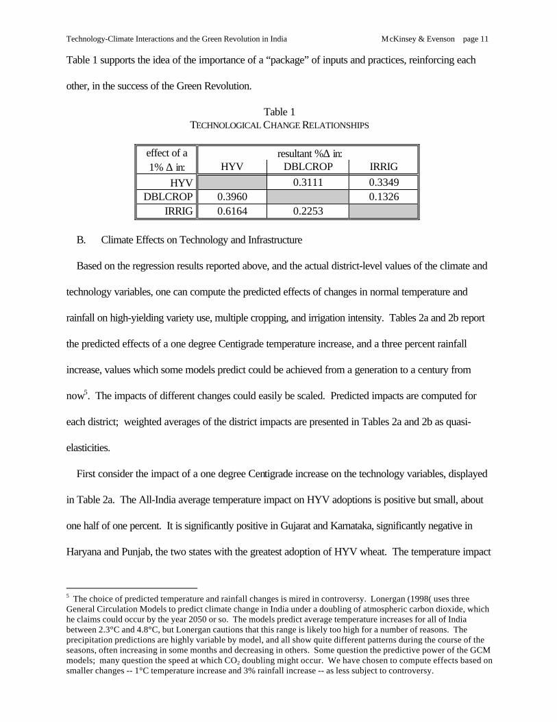
Table 1 supports the idea of the importance of a “package” of inputs and practices, reinforcing each

other, in the success of the Green Revolution.

Table 1TECHNOLOGICAL CHANGE RELATIONSHIPS

effect of a resultant %∆ in:1% ∆ in: HYV DBLCROP IRRIG

HYV 0.3111 0.3349DBLCROP 0.3960 0.1326

IRRIG 0.6164 0.2253

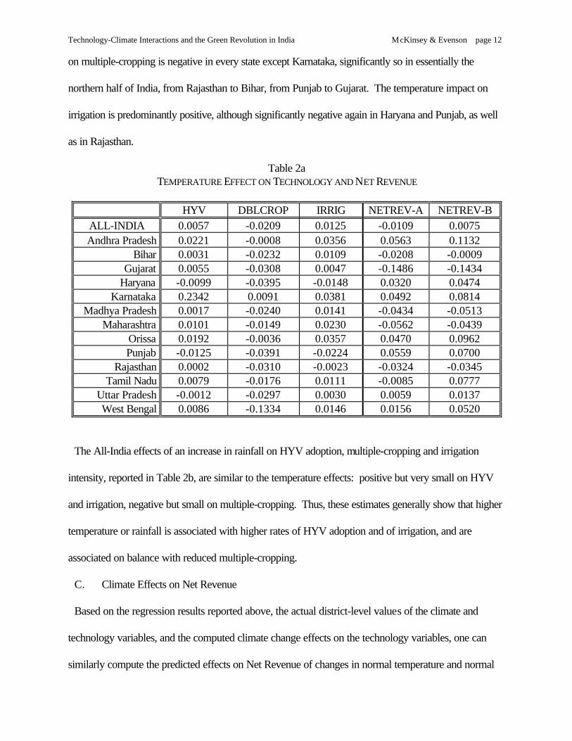
B. Climate Effects on Technology and Infrastructure

Based on the regression results reported above, and the actual district-level values of the climate and

technology variables, one can compute the predicted effects of changes in normal temperature and

rainfall on high-yielding variety use, multiple cropping, and irrigation intensity. Tables 2a and 2b report

the predicted effects of a one degree Centigrade temperature increase, and a three percent rainfall

increase, values which some models predict could be achieved from a generation to a century from

now5. The impacts of different changes could easily be scaled. Predicted impacts are computed for

each district; weighted averages of the district impacts are presented in Tables 2a and 2b as quasi-

elasticities.

First consider the impact of a one degree Centigrade increase on the technology variables, displayed

in Table 2a. The All-India average temperature impact on HYV adoptions is positive but small, about

one half of one percent. It is significantly positive in Gujarat and Karnataka, significantly negative in

Haryana and Punjab, the two states with the greatest adoption of HYV wheat. The temperature impact

5 The choice of predicted temperature and rainfall changes is mired in controversy. Lonergan (1998( uses threeGeneral Circulation Models to predict climate change in India under a doubling of atmospheric carbon dioxide, whichhe claims could occur by the year 2050 or so. The models predict average temperature increases for all of Indiabetween 2.3°C and 4.8°C, but Lonergan cautions that this range is likely too high for a number of reasons. Theprecipitation predictions are highly variable by model, and all show quite different patterns during the course of theseasons, often increasing in some months and decreasing in others. Some question the predictive power of the GCMmodels; many question the speed at which CO2 doubling might occur. We have chosen to compute effects based onsmaller changes -- 1°C temperature increase and 3% rainfall increase -- as less subject to controversy.


on multiple-cropping is negative in every state except Karnataka, significantly so in essentially the

northern half of India, from Rajasthan to Bihar, from Punjab to Gujarat. The temperature impact on

irrigation is predominantly positive, although significantly negative again in Haryana and Punjab, as well

as in Rajasthan.

Table 2aTEMPERATURE EFFECT ON TECHNOLOGY AND NET REVENUE

HYV DBLCROP IRRIG NETREV-A NETREV-BALL-INDIA 0.0057 -0.0209 0.0125 -0.0109 0.0075Andhra Pradesh 0.0221 -0.0008 0.0356 0.0563 0.1132

Bihar 0.0031 -0.0232 0.0109 -0.0208 -0.0009Gujarat 0.0055 -0.0308 0.0047 -0.1486 -0.1434

Haryana -0.0099 -0.0395 -0.0148 0.0320 0.0474Karnataka 0.2342 0.0091 0.0381 0.0492 0.0814

Madhya Pradesh 0.0017 -0.0240 0.0141 -0.0434 -0.0513Maharashtra 0.0101 -0.0149 0.0230 -0.0562 -0.0439

Orissa 0.0192 -0.0036 0.0357 0.0470 0.0962Punjab -0.0125 -0.0391 -0.0224 0.0559 0.0700

Rajasthan 0.0002 -0.0310 -0.0023 -0.0324 -0.0345Tamil Nadu 0.0079 -0.0176 0.0111 -0.0085 0.0777

Uttar Pradesh -0.0012 -0.0297 0.0030 0.0059 0.0137West Bengal 0.0086 -0.1334 0.0146 0.0156 0.0520

The All-India effects of an increase in rainfall on HYV adoption, multiple-cropping and irrigation

intensity, reported in Table 2b, are similar to the temperature effects: positive but very small on HYV

and irrigation, negative but small on multiple-cropping. Thus, these estimates generally show that higher

temperature or rainfall is associated with higher rates of HYV adoption and of irrigation, and are

associated on balance with reduced multiple-cropping.

C. Climate Effects on Net Revenue

Based on the regression results reported above, the actual district-level values of the climate and

technology variables, and the computed climate change effects on the technology variables, one can

similarly compute the predicted effects on Net Revenue of changes in normal temperature and normal


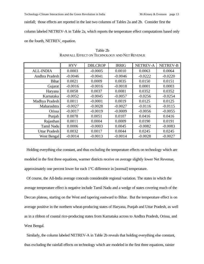
rainfall; those effects are reported in the last two columns of Tables 2a and 2b. Consider first the

column labeled NETREV-A in Table 2a, which reports the temperature effect computations based only

on the fourth, NETREV, equation.

Table 2bRAINFALL EFFECT ON TECHNOLOGY AND NET REVENUE

HYV DBLCROP IRRIG NETREV-A NETREV-BALL-INDIA 0.0003 -0.0005 0.0010 0.0063 0.0064Andhra Pradesh -0.0046 -0.0041 -0.0046 -0.0222 -0.0220

Bihar 0.0021 0.0009 0.0035 0.0150 0.0151Gujarat -0.0016 -0.0016 -0.0018 0.0001 0.0003

Haryana 0.0058 0.0037 0.0081 0.0352 0.0352Karnataka -0.0052 -0.0045 -0.0057 -0.0256 -0.0254

Madhya Pradesh 0.0011 -0.0001 0.0019 0.0125 0.0125Maharashtra -0.0027 -0.0028 -0.0027 -0.0116 -0.0115

Orissa -0.0017 -0.0019 -0.0009 -0.0056 -0.0055Punjab 0.0078 0.0051 0.0107 0.0416 0.0416

Rajasthan 0.0011 0.0004 0.0009 0.0190 0.0191Tamil Nadu 0.0006 -0.0003 0.0045 -0.0082 -0.0083

Uttar Pradesh 0.0032 0.0017 0.0044 0.0245 0.0245West Bengal -0.0014 -0.0013 -0.0014 -0.0028 -0.0027

Holding everything else constant, and thus excluding the temperature effects on technology which are

modeled in the first three equations, warmer districts receive on average slightly lower Net Revenue,

approximately one percent lower for each 1°C difference in [normal] temperature.

Of course, the All-India average conceals considerable regional variation. The states in which the

average temperature effect is negative include Tamil Nadu and a wedge of states covering much of the

Deccan plateau, starting on the West and tapering eastward to Bihar. But the temperature effect is on

average positive in the northern wheat-producing states of Haryana, Punjab and Uttar Pradesh, as well

as in a ribbon of coastal rice-producing states from Karnataka across to Andhra Pradesh, Orissa, and

West Bengal.

Similarly, the column labeled NETREV-A in Table 2b reveals that holding everything else constant,

thus excluding the rainfall effects on technology which are modeled in the first three equations, rainier


districts receive on average very slightly larger Net Revenue, less than one percent higher for each three

percent difference in (normal) rainfall.

There is dramatic regional variation in the rainfall effects, which are on average negative in the

southern, peninsular half of the subcontinent (Tamil Nadu, Orissa and West Bengal are barely negative,

while Andhra Pradesh, Karnataka and Maharashtra are more so) and positive in the northern half of the

country (Punjab, Haryana, Uttar Pradesh, and Bihar, as well as Gujarat, Rajasthan and Madhya

Pradesh).

But consider now the last columns of Tables 2a and 2b, labeled NETREV-B, which report the climate

effects computed from all four equations, including the climate effects on technology from the first three

equations working through the subsequent technology effects on Net Revenue from the fourth equation.

According to these estimates, accounting for the effects of technology would slightly mitigate the

temperature effect: it becomes barely positive on average, while the effects in Tamil Nadu go from

negative to positive and the effects in Bihar go from negative to essentially zero. In the other four states

in which the effect had been negative there is virtually no change. In the ribbon of coastal rice states the

positive effect becomes twice or thrice as large; in the northern wheat-producing states the positive

effect nearly doubles. Accounting for technology, however, does little to the rainfall effects, as seen in

comparing the last two columns of Table 2b.

The rainfall effects deserve further discussion. It is widely recognized (e.g., Gopalaswamy [1994];

Singh [1997]) that the true rainfall issue in most of India is not its average (or “normal”) amount, but

rather its timing and its variability (expressed commonly as its “unreliability”). We include variables

which measure the actual rainfall during key months of each year (June, and the sum of July and

August), as well as the coefficient of variation of rainfall during those months, in order to pick up the

timing of rainfall. Given the significance of the coefficients of these variables, and the relatively limited


role of “normal” rainfall compared to rainfall timing, it is remarkable that one would observe any

systematic “normal” rainfall effects at all.


D. Technological Change Effects on Net Revenue

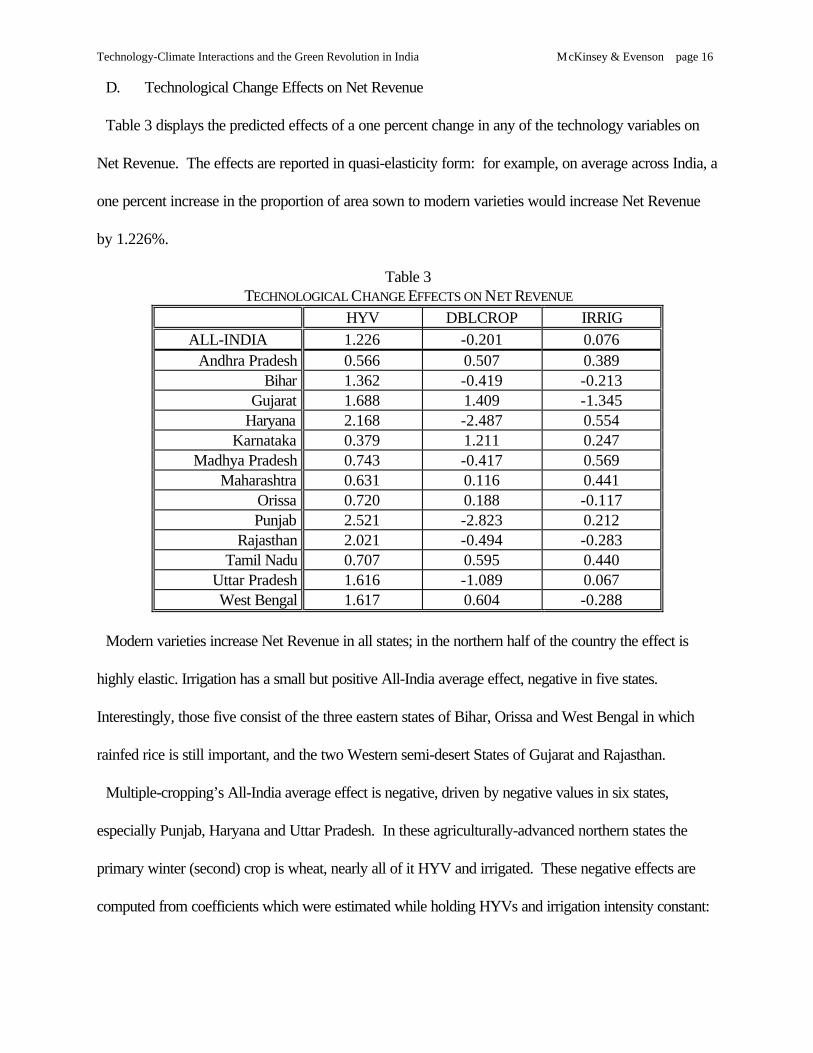
Table 3 displays the predicted effects of a one percent change in any of the technology variables on

Net Revenue. The effects are reported in quasi-elasticity form: for example, on average across India, a

one percent increase in the proportion of area sown to modern varieties would increase Net Revenue

by 1.226%.

Table 3TECHNOLOGICAL CHANGE EFFECTS ON NET REVENUE

HYV DBLCROP IRRIGALL-INDIA 1.226 -0.201 0.076

Andhra Pradesh 0.566 0.507 0.389Bihar 1.362 -0.419 -0.213

Gujarat 1.688 1.409 -1.345Haryana 2.168 -2.487 0.554

Karnataka 0.379 1.211 0.247Madhya Pradesh 0.743 -0.417 0.569

Maharashtra 0.631 0.116 0.441Orissa 0.720 0.188 -0.117Punjab 2.521 -2.823 0.212

Rajasthan 2.021 -0.494 -0.283Tamil Nadu 0.707 0.595 0.440

Uttar Pradesh 1.616 -1.089 0.067West Bengal 1.617 0.604 -0.288

Modern varieties increase Net Revenue in all states; in the northern half of the country the effect is

highly elastic. Irrigation has a small but positive All-India average effect, negative in five states.

Interestingly, those five consist of the three eastern states of Bihar, Orissa and West Bengal in which

rainfed rice is still important, and the two Western semi-desert States of Gujarat and Rajasthan.

Multiple-cropping’s All-India average effect is negative, driven by negative values in six states,

especially Punjab, Haryana and Uttar Pradesh. In these agriculturally-advanced northern states the

primary winter (second) crop is wheat, nearly all of it HYV and irrigated. These negative effects are

computed from coefficients which were estimated while holding HYVs and irrigation intensity constant:


the negative multiple-cropping coefficients and effects, then, probably reflect the revenue disadvantage

of second crops other than irrigated HYV wheat.

E. “Secondary” Effects of Technology and Climate

The presence of both technology and climate variables in our model allows us to estimate the effects

on Net Revenue of (both cross-section differences and time-series changes in) technology and (current

cross-section differences and possible future changes in) climate. The presence of variables which

measure the interaction of technology and climate allows us to estimate “secondary” effects, displayed

in Table 4, which can be interpreted from the point of view of technology’s influence on the climate

effects which are reported above in Tables 2a and 2b (the rows of Table 4), or of climate’s influence on

the technology effects which are reported above in Table 3 (the columns of Table 4).

Table 4“SECONDARY” EFFECTS

Temperature RainfallHYV 0.0663 -0.0154

DBLCROP 0.1380 -0.0007IRRIG 0.0031 0.0151

From the first point of view, technology's influence on the climate effects, Table 4 reveals that

increases in all three measures of technology -- the adoption of modern varieties, especially the

expansion of multiple-cropping, and weakly the expansion of irrigation -- would mitigate any negative

impact of higher temperatures. A one percent increase in the proportion of crops planted to modern

varieties would increase the benefit to Net Revenue of higher temperatures by about one sixteenth of

one percent; a one percent increase in the intensity of multiple-cropping would increase the benefit to

Net Revenue of higher temperatures by nearly one sixth of one percent, and a one percent increase in

irrigation intensity would increase the benefit to Net Revenue of higher temperatures by a tiny fraction of

one percent. These results confirm the differences found between columns NETREV-A and NETREV-


B in Table 2a, which showed that accounting for the beneficial effects of technology-climate interactions,

the temperature effects on Net Revenue go from slightly negative to slightly positive.

The reasons for these effects are not difficult to discern. HYV's impact on the temperature effect

derives from the success of breeders in adapting increased yield characteristics to different climatic

environments. Multiple cropping's relatively strong impact on the temperature effect captures the

benefits of shifting production of high-value crops to a second, presumably cooler, growing season

when overall temperatures are higher. And irrigation's impact on the temperature effects are nearly a

wash, probably reflecting the positive benefits of irrigation on heat stress countered by the increased

evaporation from canal and tank systems with higher temperatures.

Continuing the first point of view, technology's influence on the climate effects, Table 4 further reveals

that increases in two of the three measures of technology -- the adoption of modern varieties, and the

expansion of multiple-cropping -- would very slightly reduce the positive impact of higher rainfall, while

increases in the third, irrigation intensity, would slightly increase rainfall's positive impact. Together,

these three essentially cancel each other out, as suggested by the nearly identical values in Columns

NETREV-A and NETREV-B of Table 2b, which showed that accounting for technology left the rainfall

effects on Net Revenue virtually unchanged.

Again, the reasons for these effects are not difficult to discern. Nearly all modern varieties are highly

sensitive to precise, controlled amounts and timing of water, which is obviously best provided by reliable

irrigation systems; thus most HYVs are planted on irrigated land. Higher rainfall would likely provide

little production benefit, and often creates flooding or waterlogging which hamper timely planting and

harvesting operations or leach nutrients, reducing output and revenue. Similarly, almost all multiple-

cropping occurs on irrigated land, so although the first crop may be rainfed the second seldom is,

explaining the virtually zero effect. Irrigation's small but positive impact on the rainfall effect may derive


from the ability of some forms of irrigation to provide improved drainage, and temporary storage of

excess water.

Now considering the second point of view, climate's influence on the technology effects, Table 4

further reveals that higher temperatures would increase the benefits from investments in all three forms of

technology: that is, the payoffs to investments in improved varieties, multiple-cropping and irrigation

systems will be even higher if temperatures increase, because these technologies can mitigate any

harmful temperature impacts. However, higher rainfall would very slightly reduce the benefits of

increased adoption of modern varieties and, by about the same small proportion, very slightly increase

the benefits of increased irrigation intensity. Higher rainfall would leave the benefits of increased

multiple-cropping virtually unchanged.

VI. CONCLUSIONS

We have constructed a four-equation model of the Indian agricultural sector which is designed to

capture the major features and processes of technological and infrastructural change which have

characterized India’s Green Revolution. Each group of variables is significant and well-behaved. We

find that climate affects technology development and diffusion, and that technology development and

diffusion affects the impacts of climate on productivity in India. Technology and climate interact to affect

Net Revenue in agriculture in India.

Higher temperatures and rainfall are associated, on average across India, with slightly higher irrigation

intensity and with slightly greater adoption of modern varieties, with striking regional patterns. However,

higher temperatures and rainfall are associated with somewhat lower cropping intensity in nearly every

state of India. Because these effects are small, climate change is not expected to affect substantially the

development and diffusion of technology in Indian agriculture.

The development and diffusion of technology has a small effect on climate sensitivity as well. Increases

in the use of modern varieties and in the intensity of multiple-cropping slightly worsen (that is, reduce)


the estimated positive impacts of increases in rainfall on farm production, while increases in the intensity

of irrigation would increase the benefits of increased rainfall. Increases in the use of modern varieties, in

the intensity of irrigation, and especially in the intensity of multiple-cropping mitigate or improve the

effects of an increase in temperature. Alternatively interpreted, increases in temperature would slightly

increase the payoff to investments in technology and infrastructure, while increases in rainfall would

slightly increase the payoff to investments in irrigation, and slightly reduce the payoffs to investments in

modern varieties and to increases in multiple-cropping.

Finally, most global climate change scenarios also posit an increase in atmospheric carbon –– usually,

in fact, the climate change is initiated by an increase in atmospheric CO2. Nearly every experimental

crop model predicts higher crop yields associated with increases in available carbon. For example, de

Siqueira et al [1994] used crop growth models developed by IBSNAT and calibrated for thirteen

regions in Brazil, to simulate climate change effects on wheat, maize and soybean production. The crop

growth models allowed simulation of the direct physiological effect of increases in atmospheric

concentrations of CO2 on photosynthesis and the efficiency of water use. They found that, ignoring the

effect of CO2, a 2°C increase in temperature would increase soybean production but would reduce

wheat and maize production. However, doubling CO2 concentrations (by 555 ppm) increased output

of all three crops, essentially compensating for the negative temperature impact on wheat and maize.

This study deals with changes in temperature and rainfall, but not with changes in carbon; thus the

actual effects on crop output [and thus on Net Revenue] of climate change, taking into account carbon

changes as well as temperature and rainfall changes, would almost certainly be more beneficial than the

results of this study predict.


Appendix Table A-1Variable Dictionary

Variable Standard Name Description Mean Deviation

A. ENDOGENOUS VARIABLESNETREV Log of Deflated Net Revenue 5.57 .74HYV % of Land Planted to High-Yielding Varieties .28 .25DBLCROP Multiple-Cropping Index 1.24 .20IRRIG Index of Irrigation Intensity .29 .24

B. EXOGENOUS VARIABLES Edaphic Variables [EDAPH]DMSnn * Soil Type Dummy Variables; nn: 03 to 21 -- --DMpHn Soil pH Dummy Variables; n: 5, 6, 8 and 9 -- --DMTSn * Topsoil Depth Dummy Variables; n: 1, 2 and 3 -- --

Geographic VariablesDMSLPn Slope Dummy Variables; n: 1 to 4 -- --DMSEA Dummy: 1 if District is on the seacoast -- --DMSEANEI Dummy: 1 if District abuts one on seacoast -- --ALT Altitude of District’s weather station, meters 296.89 316.36DMAQn Aquifer Depth Dummies -- --

[Normal] Climate Variables [CLIMATE]JANTEMP* January Normal Temperature Midpoint [°C] 18.55 3.69JANTEMPSQ* January Normal Temp. Midpoint Squared [°C] 357.86 138.29JANRAIN* January Normal Rainfall [mm] 12.38 13.14JANRAINSQ* January Normal Rainfall Squared [mm] 325.75 725.31JANTMPRN* January Normal Temp. times RainfallAPRTEMP* April Normal Temperature Midpoint [°C] 29.59 2.35APRTEMPSQ* April Normal Temp. Midpoint Squared [°C] 881.23 125.86APRRAIN* April Normal Rainfall [mm] 16.19 22.65APRRAINSQ* April Normal Rainfall Squared [mm] 775.13 2355.60APRTMPRN* April Normal Temp. times RainfallJULTEMP* July Normal Temperature Midpoint [°C] 28.34 2.55JULTEMPSQ* July Normal Temp. Midpoint Squared [°C] 809.90 134.44JULRAIN* July Normal Rainfall [mm] 245.77 234.42JULRAINSQ* July Normal Rainfall Squared [mm] 115342.86 430432.59JULTMPRN* July Normal Temp. times RainfallOCTTEMP* October Normal Temperature Midpoint [°C] 26.05 1.88OCTTEMPSQ* October Normal Temp. Midpoint Squared [°C] 682.01 90.17OCTRAIN* October Normal Rainfall [mm] 66.64 66.03OCTRAINSQ* October Normal Rainfall Squared [mm] 8800.36 15815.10OCTTMPRN* October Normal Temp. times RainfallJURNCV Coef. of Variation, June Rain, 1957 - 1987 .61 .21JARNCV Coef. of Var., July/Aug Rain, 1957 - 1987 .35 .21


Appendix Table A-1 (continued)Variable Dictionary

Variable Standard Name Description Mean Deviation

[Current] Weather Variables [W]JUNERAIN Actual Rainfall in June [mm] 131.46 121.98JUAURAIN Actual Rainfall in July and August [mm] 561.55 364.05YEARRAIN Actual Annual Rainfall [mm] 1088.33 602.14

Additional Technology and Infrastructural Variables [T, I]RESEARCH Cumulated Stock of Public Agri. Research 36.30 43.15EXT * Index of Extension Activity 7.39 5.65LITERACY * Literacy Rate, Adult Rural Males .37 .11RELWAGE Ratio of Rural Factory Wage to Farm Wage 1.20 .60PRIVRES Private Research 247.94 187.08

Institutional VariablesPRWTWG * Price Ratio: Wheat to Wage 28.52 14.41PRRCWG * Price Ratio: Rice to Wage 28.60 17.76PRMZWG * Price Ratio: Maize to Wage 20.86 9.77PRJWWG * Price Ratio: Jowar to Wage 19.63 13.19PRBJWG * Price Ratio: Bajra to Wage 19.09 12.34PRFRWG * Price Ratio: Fertilizer to Wage 683.69 301.06PRTRWG * Price Ratio: Tractor to Wage 2309.40 811.41POPDEN1 Population Density: 3948.41 2717.01

Interaction TermsJANTEMPHY January temperature times Predicted HYVJANTEMPDB January temperature times Predicted DBLCROPJANTEMPIR January temperature times Predicted IRRIGJANRAINHY January rainfall times Predicted HYVJANRAINDB January rainfall times Predicted DBLCROPJANRAINIR January rainfall times Predicted IRRIG and similarly for April, July and October

* Variables used as instruments in the first stage of HYV, DBLCROP and IRR regressions.


Appendix Table A-2Regressions of HYV, DBLCROP, IRRIG and NETREV

HYV DBLCROP IRRIG NETREVR-sq 0.7274 0.6986 0.9019 0.5273

Root MSE .1248 .1058 .0741 .5130F 166.16 294.40 740.34 43.80

HYV DBLCROP IRRIG NETREVcoeff. t coeff. t coeff. t coeff. t

(constant) -.9029 -2.176 -.9233 -3.358 .4022 1.693 -1.792 -0.355

HYV .2945 15.995 .3349 26.910 .0106 .0005

DBLCROP .3960 3.870 -2.2190 -0.627

DBLCROP57 .4158 14.097

IRRIG .5968 8.495 .0495 2.137 -.5383 -0.225

IRRIG57 .7611 61.478

RESEARCH .0011 2.471 .0022 4.394

EXT .0107 7.223

RES x EXT -.0001 -2.346

PRIVRES .0001 3.748 .0008 4.605

DMSLP1 .0501 6.580 .0255 4.383

DMSLP2 .0141 1.875 -.0157 -2.802

DMSLP3 .0196 1.931 -.0062 -1.130

DMSLP4 .0950 7.701 -.0231 -2.997

DMAQ1 .0036 0.835

DMAQ2 .0052 0.991

DMAQ3 .0250 3.557

DMPH5 -.0476 -1.266

DMPH6 -.0484 -1.522

DMPH8 -.1919 -6.128

DMPH9 -.2997 -6.822

ALT .0007 0.483

CULTIVAT .1534 4.930

BULLOCK -.1298 -4.600

RELWAGE -.0951 -3.271

DMSEA .0192 0.269

DMSEANEI .1098 2.565

––––> Appendix Table A-2 is continued on the next page


Appendix Table A-2 (continued)Regressions of HYV, DBLCROP, IRRIG and NETREV


DMS03 -.0215 -1.610 .0173 2.078 -.0054 -.0915 .1222 2.269

DMS04 -.0101 -1.210 -.0059 -0.772 -.0144 -.2588 .0233 0.427

DMS05 .0295 4.109 -.0032 -0.589 -.0058 -.1467 -.0974 -2.265

DMS06 .0007 0.095 .0211 4.467 .0058 1.397 -.0683 -1.393

DMS07 -.0341 -4.774 -.0110 -1.307 -.0007 -.0127 .0496 1.321

DMS08 .0268 1.455 -.1414 -9.183 -.0305 -3.456 .2147 2.129

DMS09 .0213 1.452 -.1118 -11.82 -.0409 -5.062 -.2079 -2.308

DMS10 -.0111 -0.282 .0402 1.963 -.0452 -2.105 -.7358 -4.341

DMS11 .0776 4.475 -.0691 -5.759 -.0111 -1.148 -.3019 -2.020

DMS12 .0179 0.908 .0329 2.548 -.0918 -8.161 -.4180 -4.408

DMS13 -.2299 -10.42 .0006 0.050 .1633 14.711 .5438 5.494

DMS14 -.0175 -1.288 -.0162 -1.672 -.0417 6.628 -.2147 -2.520

DMS15 -.0222 -1.703 -.0002 -0.026 .0360 5.027 .0272 0.613

DMS16 .0379 5.156 -.0038 -0.646 .0128 2.824 -.0120 -0.328

DMS17 .0253 2.173 .0145 1.642 -.00002 -0.003 -.3421 -3.716

DMS18 -.3234 -8.118 .3041 9.399 .1263 7.715 .3227 2.248

DMS19 -.1010 -9.905 .0383 5.021 .0142 3.148 -.0665 -1.609

DMS20 .0365 1.944 -.0426 -5.251 -.0220 -2.892 -.2069 -2.451

DMS21 .2671 7.882 -.0704 -4.384 -.0025 -0.133 -.4506 -2.863

JANTEMP .0693 3.720 .0342 3.431 -.0714 -8.412 .2462 1.673

JANTEMPSQ -.0015 -3.126 -.0012 -4.940 .0019 9.125 -.0056 -2.538

JANRAIN -.0013 -0.832 .0023 1.486 .0051 6.019 .0077 2.637

JANRAINSQ .0001 8.169 .00004 2.872 -.0001 -8.217 .0004 5.666

JANTEMPRN .0002 -2.522 -.0003 -4.214 -.0001 -2.787 -.0034 -6.137

APRTEMP -.1131 -3.740 .0211 0.912 .1711 9.927 -.3175 -1.244

APRTEMPSQ .0022 4.147 -.0008 -1.918 -.0030 -10.26 .0022 0.757

APRRAIN .0099 4.022 .0066 3.780 -.0054 -3.958 .0148 0.904

APRRAINSQ -.00002 -4.897 -7.3E-6 -1.687 3.9E-6 1.374 -.0001 -5.269

APRTEMPRN -.0002 -2.967 -.0002 -3.535 .0001 2.991 -.0010 -2.615

JULTEMP .1990 4.186 .1398 5.925 -.2139 -9.606 .6178 2.341

JULTEMPSQ -0033 -3.880 -.0027 -6.364 .0038 9.712 .015 0.396

JULRAIN .0007 3.997 .0003 2.654 -.0003 -2.547 .0087 6.600

JULRAINSQ -6.3E-8 -3.098 -8.6E-9 -0.482 1.2E-8 0.767 -3.8E-7 -2.352

JULTEMPRN -.00002 -3.118 -.00001 -2.424 7.4E-6 1.898 -.0002 -4.915

OCTTEMP -.1108 -2.539 -.0464 -1.564 .0404 1.886 .1122 0.283

OCTTEMPSQ .0014 1.757 .0012 2.119 -.0003 -0.676 -.0167 -3.372

OCTRAIN -.0062 -3.928 -.0063 -7.842 .0053 9.055 -.0297 -3.729

OCTRAINSQ -1.7E-6 -1.765 -1.3E-6 -2.304 -5.9E-7 -1.507 -.00001 -3.636

OCTTEMPRN .0002 3.837 .0002 8.108 -.0002 -9.032 .0016 6.544


Appendix Table A-2 (continued)Regressions of HYV, DBLCROP, IRRIG and NETREV


JUNERAIN -.00004 -0.301

JUAURAIN .0002 2.945

YEARRAIN .00007 1.313

JURNCV .2051 2.210

JARNCV .5657 7.310

JANTEMPHY -.0028 -0.039

JANTEMPDB -.0979 -0.999

JANTEMPIR .2364 2.630

JANRAINHY -.0180 -2.017

JANRAINDB -.0161 -1.022

JANRAINIR -.0048 -0.485

APRTEMPHY -.3398 -4.178

APRTEMPDB .1291 0.946

APRTEMPIR .2578 2.361

APRRAINHY .0040 0.543

APRRAINDB .0253 3.156

APRRAINIR .0139 1.872

JULTEMPHY .2907 2.768

JULTEMPDB -.7432 -5.142

JULTEMPIR .5306 4.502

JULRAINHY .0014 3.090

JULRAINDB -.0034 -3.398

JULRAINIR .0009 1.065

OCTTEMPHY .1182 0.740

OCTTEMPDB .8500 3.677

OCTTEMPIR -1.0217 -5.780

OCTRAINHY -.0027 -1.103

OCTRAINDB -.0065 -1.715

OCTRAINIR -.0034 -0.994



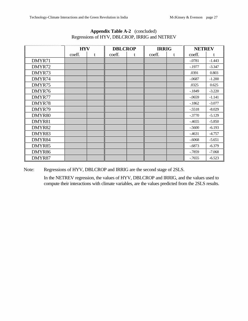
Appendix Table A-2 (concluded)Regressions of HYV, DBLCROP, IRRIG and NETREV


DMYR71 -.0781 -1.443

DMYR72 -.1977 -3.347

DMYR73 .0391 0.803

DMYR74 -.0687 -1.200

DMYR75 .0325 0.625

DMYR76 -.1849 -3.220

DMYR77 -.0659 -1.141

DMYR78 -.1862 -3.077

DMYR79 -.5518 -8.029

DMYR80 -.3770 -5.129

DMYR81 -.4655 -5.850

DMYR82 -.5600 -6.193

DMYR83 -.4631 -4.757

DMYR84 -.6068 -5.651

DMYR85 -.6873 -6.379

DMYR86 -.7859 -7.068

DMYR87 -.7655 -6.523

Note: Regressions of HYV, DBLCROP and IRRIG are the second stage of 2SLS.

In the NETREV regression, the values of HYV, DBLCROP and IRRIG, and the values used tocompute their interactions with climate variables, are the values predicted from the 2SLS results.


REFERENCES

de Siqueira, Otavio Joao Fernandes, Jose Renato Boucas de Farias and Luiz Marcelo Aguiar Sans, 1994,“Potential Effects of Global Climate Change for Brazilian Agriculture and Adaptive Strategies forWheat, Maize and Soybean”, Revista Brasileira de Agrometeoroligia, vol.2, pp. 115-129

Evenson, Robert E., and James W. McKinsey, Jr., 1991, “Research, Extension, Infrastructure, andProductivity Change in Indian Agriculture”. Chapter 6 in Research and Productivity in AsianAgriculture, Robert E. Evenson and Carl E. Pray, eds., Ithaca, NY: Cornell University Press

Evenson, Robert E., Carl E. Pray and Mark Rosegrant, 1999, Agricultural Research and ProductivityGrowth in India, Research Report # 109, International Food Policy Research Institute, Washington,DC

Gopalaswamy, N., 1994, Agricultural Meteorology, Jaipur, Rawat Publications

Intergovernmental Panel on Climate Change (IPCC), 1996, Climate Change 1995: The Science ofClimate Change. World Meteorological Organization of the United Nations Environment Programme,Cambridge: Cambridge University Press

Kumar, K. S. Kavi, and Jyoti Parikh, 1998, “Climate Change Impacts on Indian Agriculture: TheRicardian Approach”, in Measuring the Impact of Climate Change on Indian Agriculture, ArielDinar et. al., World Bank Technical Paper # 402, The World Bank, Washington, D.C.

Lonergan, Steve, 1998, “Climate Warming and India”, in Measuring the Impact of Climate Change onIndian Agriculture, Ariel Dinar et. al., World Bank Technical Paper # 402, The World Bank,Washington, D.C.

McKinsey, James W., Jr., 1998, HYVs, Multiple-Cropping, Irrigation, Climate and the GreenRevolution in India. Unpublished Ph.D. Dissertation, Yale University

McKinsey, James W., Jr., and Robert E. Evenson, 1998, “Technology - Climate Interactions: Was theGreen Revolution in India Climate Friendly?” in Measuring the Impact of Climate Change on IndianAgriculture, Ariel Dinar et. al., World Bank Technical Paper # 402, The World Bank, Washington,D.C.

Mendelsohn, Robert, William Nordhaus and Dai Gee Shaw, 1994 , “The Impact of Global Warming onAgriculture: A Ricardian Analysis”, American Economic Review (84:753-771, September)

William Nordhaus and Ferene Toth, eds., Costs, Impacts and Benefits of CO2 Mitigation Laxemburg,Austria: International Institute of Applied Systems Analysis, pp. 173-208

Mendelsohn, Robert, William Nordhaus and Dai Gee Shaw, 1994, “The Impact of Global Warming onAgriculture: A Ricardian Analysis” American Economic Review (84:753-771, September 1994)


Parikh, K.S., 1994, “Agriculture and food System Scenarios for the 21st Century,” in Agriculture,Environment and Health: Sustainable Development in the 21st Century, Vernon W. Ruttan, ed.,Minneapolis: University of Minnesota Press

Rosenzweig, Cynthia and A. Iglesias, eds., 1994, Implications of Climate Change for InternationalAgriculture: Crop Modeling Study. United States Environmental Protection Agency, June.

Rosenzweig, Cynthia, M. L. Parry, G. Fischer, and K. Frohberg, 1993, Climate Change and WorldFood Supply. Research Report # 3, Environmental Change Unit, University of Oxford

Sanghi, Apurva, Robert Mendelsohn & Ariel Dinar, 1998, “The Climate Sensitivity of Indian Agriculture”,in Measuring the Impact of Climate Change on Indian Agriculture, Ariel Dinar et. al., World BankTechnical Paper # 402, The World Bank, Washington, D.C.

Segerson, Kathleen, and Bruce L. Dixon, 1996, Climate Change and Agriculture: The Role of FarmerAdaptation, Revised Final Report to EPRI, June 1996

Singh, Jasbir, 1997, Agricultural Development in South Asia, National Book Organisation, New Delhi

Winters, P., R. Murgai, Alain de Janvry, E. Sadoulet, and G. Frisvold, 1994, “Climate Change andAgriculture: An Analysis of the Effects on Developing Economies”, paper presented at GlobalEnvironmental Change and Agriculture: Assessing the Impacts, Economic Research Service andthe Farm Foundation Conference, Rosslyn, VA

TECHNOLOGYâ€“CLIMATE INTERACTIONS IN THE GREEN REVOLUTION IN INDIA

Documents

Transcript of TECHNOLOGYâ€“CLIMATE INTERACTIONS IN THE GREEN REVOLUTION IN INDIA