Technology Spillover Effects and Economic Integration -...

Technology Spillover Effects and Economic Integration:

Evidence from Integrating Countries

Kurt A. Hafner*

August 2012

University of Heilbronn, Germany

Abstract

The paper focuses on the impact of R&D expenditure on labor productivity of economically

integrating countries using patent-, trade- and FDI-related technology diffusion channels.

Time series for Greece, Ireland, Portugal and Spain representing European integration and for

Mexico joining the free trade agreement with the USA and Canada are based on a set of 32

OECD countries for a time period from 1981 to 2008. Accounting for nonstationary data and

cointegration, the paper uses the single equation EC model and finds empirical evidence for

foreign technology spillover effects for Ireland (patent- and trade-related), Portugal (patent-

related) and Spain (FDI-related). Moreover, there are significant impacts of foreign technolo-

gy spillover effects for Ireland and Portugal from European economic integration no matter if

technology diffusion is restricted to EU-12 or EU-15 countries, whereas for Mexico no such

evidence from joining NAFTA is found.

JEL Classification: C22, O30, R12

Keywords: Technology Diffusion, Economic Integration, Nonstationary Time Series,

Cointegration, Single Equation EC Model

* Hafner: University of Heilbronn, Department W2, Max-Planck-Straße 39, 74081 Heilbronn,

Germany. Tel: +49-7131-504516; Fax: +49-7131-252470; Email: kurt.hafner@hs-

heilbronn.de.

2

1 Introduction

In May 2004 and January 2007, Central and Eastern European Countries joined the European

Union (EU) thus augmenting the membership to 27 countries. In the decades before, several

waves of integration steadily increased the number from originally six founding members in

1957 to 15 member countries by the end of the last century. Amongst the first countries to

join the post-formed European Community were Greece, Ireland, Portugal and Spain, which

experienced a remarkable economic development since then and prior to the financial crisis in

2008/2009. Moreover, the North American Free Trade Agreement (NAFTA) between the

USA, Canada and Mexico became effective by January 1994 allowing goods, capital and (to

some degree) factors to flow almost freely. According to Hufbauer and Schott (1993),

NAFTA was the first reciprocal free trade agreement between a developing country and de-

veloped countries outside the EU. Since then Canada and Mexico have become the US’s first

and second largest trading partner respectively with a direct impact on the US-economy rang-

ing from relocation of industrial activity towards the US-Mexican border to outsourcing of

labor-intensive production to Mexico.

Economic integration seems to benefit acceding countries in catching up economically.

However, it is not the only source of growth and prosperity. Following Keller (2004), the

adoption of foreign technology is understood to promote and strengthen economic develop-

ment as well. Again, further economic integration may spur technology diffusion through a

tighter relationship, but not necessarily. Bilateral trade, for example, is considered to transfer

technology between trading countries regardless of geographical proximity. If technology is

mainly embedded in intermediate goods, then trade in intermediate goods gives countries

access to foreign know-how. Multinational firms, as another example discussed by Kleinert

and Tobal (2010), diffuse technological know-how and technology through FDI and their

affiliates abroad. And finally, the pattern of international patenting according to Eaton and

Kortum (1999) indicate of where ideas are going and therefore reflect the link between the

source and the destination of transferred technology. Since relationships between countries

are getting closer within economically integrating regions, spatial integration and technology

diffusion lead to self-reinforcing processes spurring and fostering economic development.

According to Keller (2004) empirical work looking for macro (and micro) evidence for

technology spillover effects is mainly based on bilateral trade and FDI as traditional ap-

proaches like in Coe and Helpman (1995) and Branstetter (2005) rather than on foreign pa-

tents. Studies from Jaffe and Trajtenberg (2002) and Hafner (2008) use the pattern of interna-

3

tional patenting to determine the flow of technology but ignore the impact of economic inte-

gration on acceding countries. To address these issues, the paper uses time series based on a

set of 32 OECD countries for the period 1981-2008 and refers these to Greece, Ireland, Portu-

gal and Spain representing European integration and to Mexico joining the free trade agree-

ment with the USA and Canada. The empirical analysis focuses on the impact of R&D ex-

penditure on labor productivity and uses patent-, trade- and FDI-related technology diffusion

channels. It is tested first if the time series are of the same integrated order and second if

cointegration relationships amongst two or more time series exists. In cases where time series

are near integrated, and cointegration might or might not exist, the use of Engle and Granger

(1987)’s two-step EC model becomes problematic and estimation results are likely to be

spurious. To avoid such problems, dynamic single equation regressions like ADL models or–

equivalent–single equation EC models leads to unbiased estimates of long-run relationships.

The paper is organized as follows. The next section reviews the literature on technology

spillover effects. Section 3 outlines the theoretical framework, whereas Section 4 discusses

the data. Nonstationary issues and estimation techniques are covered in Section 5. The results

of the testing procedures and empirical estimations are given in Section 6. Section 7 presents

conclusions.

2 Technology Spillover Effects

Are international R&D spillovers trade-related and is technology mainly embodied in inter-

mediate goods? Coe and Helpman (1995), among others, confront this question empirically

by relating the direction of technology diffusion to bilateral trade shares and analyzing the

impact on total factor productivity (TFP) of a panel of 22 OECD countries over 1971-90.

They find that trade-related spillover effects are present and are stronger the more open an

economy to international trade and that causation runs mainly from R&D to productivity than

vice versa. Keller (1998), however, shows by Monte Carlo simulations that randomly created

bilateral trade patterns explain more of the variation in TFP than those empirically observed.

Additionally, long-run trended data such as productivity and R&D expenditure require appro-

priate estimation techniques to avoid spurious results. In applying a more sophisticated esti-

mation technique on the data set of Coe and Helpman (1995) and through re-examining their

econometric findings, Kao, Chiang and Chen (1999) confirm the impact of domestic R&D on

TFP but reject any diffusion of foreign technology. Recently, Savvides and Zachariadis

(2005) find in their study with a panel of 32 countries for the period 1965-92 that foreign

4

R&D has the biggest impact on domestic productivity if technology is embedded in interme-

diate goods rather than in capital goods or FDI. Kramer (2010) comes to the same result using

a panel with 47 countries for the period 1990-2006 and applying panel unit roots and

cointegration techniques. Moreover, the same study concludes that transition countries from

Eastern Europe and Central Asia have higher productivity gains from international technology

diffusion than Western countries. At the country study level, empirical work on trade-related

spillover effects, for example, have been done for Malaysia by Ghatak, Milner and Utkulu

(1997), for Taiwan by Biswal and Dhawan (1998) and for Mexico by Cabral and Mollick

(2011). In particular, the first two studies confirm at the macro level learning-by exporting

spillovers dealing with East and Southeast Asia’s export success, whereas the latter study

suggests at the micro level an increase of technology spillovers on Mexican manufacturing

productivity from joining NAFTA. While there might be a theoretical consensus about trade-

related spillover effects and the importance of a country’s openness to trade, empirically it

seems to be difficult to quantify the extent and direction of technology diffusion from trade.1

The same criticism applies to a second strand of the literature that considers FDI as a

channel for technology diffusion. Following Keller (2004), such subsidiaries might pick up

new technologies from their host countries (outward FDI technology transfer) or provide

technology to domestic firms (inward FDI technology transfer). Much of the literature on FDI

spillovers uses micro (firm or plant level) data and account for heterogeneity across sectors

and firms within a country. Recently, empirical micro evidence for economically important

FDI spillover effects have been found by Haskel, Pereira, and Slaughter (2002) for the United

Kingdom, by Keller and Yeaple (2009) for the United States and by Khalifah and Adam for

Malaysia (2009). Evidence for FDI spillover both from and to investing Japanese firms in the

United States is found by Branstetter (2005). However, studies that use both bilateral trade

and FDI as technology diffusion channels like in Savvides and Zachariadis (2005) and Kra-

mer (2010) usually find trade-related rather than FDI-related spillover effects.

Turning to foreign patents as an alternative diffusion channel to the traditional approach-

es, the pattern of international patenting according to Eaton and Kortum (1999) indicate of

where ideas are going and therefore reflect the link between the source and the destination of

transferred technology. The idea is that patenting domestic research efforts abroad determines

the transfer of technology. Local firms may take legal advantage of patented foreign

knowledge by paying royalties. Adding foreign knowledge to a country’s own R&D stock,

1 Unel (2010), for example, shows recently by a product innovation growth model that exposure to trade leads to an increase of average productivity model, but has an ambiguous effect on economic growth.

5

even in the case of limited domestic R&D spending, is likely to increase the efficiency of

domestic input factors. In particular, international patent statistics by the World Intellectual

Property Organization (WIPO) and OECD usually provide count numbers, whereas specific

information about the value of patents is not given. However, some patents are more valuable

and their economic impact differs between countries. Hence, using patent count data may

serve to determine the direction rather than the magnitude of international technology diffu-

sion. In this context, international spillover effects are patent-related. Hafner (2008) find that

patent-related spillover effects are present for a panel of 18 OECD countries over 1981-2001.

The same study shows that there are no significant spillover effects from bilateral trade, but

confirm the impact of FDI on domestic labor productivity. Moreover, the study from Xu and

Chiang (2005) confirms significant spillover effects from foreign patents and imported capital

goods for middle-income countries, whereas low-income countries benefit mainly from pa-

tent-related spillover effects. At the country study level, Branstetter and Sakakibara (2001)

find no empirical evidence in the case of Japan that stronger patents induce more innovation

and therefore more patents.

While each study offers fruitful insights on foreign spillover effects given their specifics

of data selection and estimation techniques, this paper quantifies the impact of technology

diffusion on labor productivity of economically integrating countries using patent-, trade- and

FDI-related technology diffusion channels. Hence, foreign spillover effects are not restricted

to a specific diffusion channel. Since relationships between countries are getting closer within

economically integrating regions like the EU and NAFTA, the paper focuses on the interac-

tion of spatial integration and technology diffusion by analyzing foreign technology spillover

effects from economic integration.

3 Theoretical Framework

This section outlines the theoretical framework. To quantify the impact of foreign technology

diffusion, one can divide the available capital stock of R&D (A) in country i (or its technolog-

ical knowledge) according to:

( )f

ti

d

titi SSA ,,, += , (1)

where d

tiS , and ∑≠

Γ=ij

d

tjtji

f

ti SS ,,, (for Nj ,...,1= ) represents domestic (d) and foreign (f) R&D

capital stocks (S) used in country i at time t respectively. Note that jiΓ defines country j’s

6

technology diffusion rate to country i. Hence, tiA , is determined by domestic and foreign

R&D, the latter according to the technological spillover effect and its diffusion channel.

Next, aggregated production function using the income approach in its simplest form is

given by:

),(* ,,,, titititi LKFAY = , (2)

where tiY , is the aggregate output, tiK , is the capital stock, and tiL , is the workforce. Hence,

an increase of domestic and foreign R&D expenditure leads to higher R&D capital stocks,

which–used as a proxy for the unobservable tiA , –augments the efficiency of input factors in

final output production. As a result, domestic output is likely to increase. Following Coe and

Helpman (1995), one can define total factor productivity as aggregated output divided by the

functional form of input factors to estimate the impact of foreign technology diffusion on

economic development. However, total factor productivity figures are susceptible to calcula-

tion and measurement errors and estimated coefficients might be less reliable due to inherent

biases. Due to the more reliable data on labor input and to a lack of data for an adequate stock

of business sector capital, labor productivity (LP) figures are used.2 Hence, substitution of

equation (1) in equation (2) and taking the logarithm leads to:

f

ti

d

titititi SSLPLFY ,,,,, logloglog))(/(log +=≡ . (3)

Note that the right hand side of equation (3) is a proxy for the unobservable technological

knowledge tiA , .

R&D Capital Stocks

With respect to the domestic R&D capital stock of country i, the paper follows Coe and

Helpman (1995) and uses the perpetual inventory method proposed by Griliches (1979) to

convert R&D flow (expenditure) figures (F) into R&D stock variables (S):

d

ti

d

ti

d

ti FSS 1,1,, )1( −− +−= δ , (4)

2 Coe and Helpman (1995) assume a Cobb-Douglas functional form with constant returns and define total factor productivity as output divided by the elasticity weighted input factors labor and capital. To keep the analysis comparable, aggregated output is only produced by labor and therefore by a single input factor in this paper.

7

where δ is the time- and country-invariant depreciation rate. Hence, the domestic R&D

capital stock of country i in period t is calculated by the depreciated R&D capital stock plus

the R&D flow (expenditure) of t-1. Note that the benchmark d

iS 0, for the subsequent stock data

is calculated by the first flow figure, for which the data is available, divided by its annual

growth rate and depreciation rate. Detailed information is given in Table A.1 in the appendix.

Turning to the foreign R&D capital stock of country i, definitions of f

tiS , differ according

to the diffusion channel. Hence, foreign R&D capital stocks are related first to foreign patent

applications (P), second to bilateral trade (M) and third to FDI (F).

For patent-related spillover effects, foreign R&D capital stock Pf

tiS,

, is defined as the pa-

tent weighted average of domestic R&D capital stocks from abroad:

)(1

,,

,

,

,,

d

tj

ij

tji

ij

tji

Pf

ti

f

ti Saa

SS ∑∑ ≠

≠

=≡ , Nj ,...,1= , (5)

where tjia , is country j’s patent application in country i. Note that the ratio of ∑≠ij

tjitji aa ,, /

defines the patent-related diffusion channel PΓ for country i.

To capture trade-related spillover effects, the paper follows Coe and Helpman (1995) and

define foreign R&D capital stock Mf

tiS,

, to be the average of domestic R&D capital stocks from

abroad weighted by bilateral import shares:

)(1

,,

,

,

,

,, ∑∑ ≠

≠

=≡ij

d

tjtji

ij

tji

ti

Mf

ti

f

ti Smm

MSS , Nj ,...,1= , (6)

where tjim , is country i’s import from country j. Again, the ratio of ∑≠ij

tjitji mm ,, / defines the

trade-related diffusion channel MΓ for country i. Moreover, Coe and Helpman (1995) also

propose the use of an additional measure to capture technology intensity and therefore open-

ness to trade. Hence, a country that imports more relative to its GDP (i.e. tititi YmM ,,, /= )

should benefit more from foreign R&D spillover effects, thus given the same composition of

imports and a similar trade pattern between countries.

8

The procedure to determine foreign R&D capital stocks Ff

tiS,

, differs in the case of FDI-

related spillover effects due to the lack of adequate bilateral FDI inflow data. Instead of calcu-

lating technology diffusion channels and relating them to domestic R&D capital stocks from

abroad, aggregate FDI inflow figures to calculate FDI inflow stocks are used according to:

∑≠

−− +−=≡ij

tji

Ff

ti

Ff

ti

f

ti FDISSS 1,

,

1,

,

,, )1( δ , Nj ,...,1= , (7)

where tjiFDI , is foreign direct investment from country j to country i and δ is the time- and

country-invariant depreciation rate. Again, the perpetual inventory method proposed by

Griliches (1979) is used to calculate the benchmark Ff

iS,

0, for subsequent FDI inflow stocks as

shown in Table A.2 in the Appendix.

4 The Data

The data used to measure the impact of technology diffusion and economic integration for

Greece, Ireland, Portugal and Spain and for Mexico is based on a set of 32 OECD countries

for a time period from 1981 to 2008. Availability of data reduces the number of observations

respectively. According to the literature, I use worked hours as labor input to determine labor

productivity. Figures on labor productivity per hour worked in constant 2009 US$ (constant

prices and PPP) are from the Total Economy Database, provided by the Groningen Growth

and Development Center (GGDC (2010)). Following Coe and Helpman (1995), I calculate

labor productivity as indexed figures with 2005 being the reference year.

The OECD has published data on business-related R&D expenditure (BERD) since about

1965 mainly for the G7 countries as well as for Switzerland. In order to get a data set for all

OECD countries from 1965 onwards, one has to estimate missing R&D expenditure figures as

Coe and Helpman (1995) did. However, the lack of R&D data (as well as missing patent

figures) limits the analysis to 32 OECD countries )32( =N3 and to 1982 and 2008 for

Greece, to 1981 and 2008 for Ireland, Portugal, and Spain and to 1989 and 2007 for Mexico.

As a benchmark, technology diffusion is neither limited to the European core countries in the

case of the European acceding countries nor to the USA and Canada in the case of Mexico.

However, in quantifying the impact of economic integration, I restrict technology diffusion

for the European countries first to EU-12 countries and second to EU-15 countries, and for

3 There is no sufficient data for Chile and Estonia, which reduces the number of current 34 OECD countries accordingly.

9

Mexico first to the USA and second to the USA and Canada. R&D expenditure flows are

converted into R&D capital stocks using the perpetual inventory method suggested by

Griliches (1979). R&D expenditure data in million constant 2000 US$ (constant prices and

PPP) is from the OECD (2010a) Main Science and Technology Database.

As discussed above, the paper uses country specific patent data as one of the main tech-

nology diffusion channels. Since 1975 the World Intellectual Property Organization (WIPO)

offered in its Industrial Property Statistics Publication B Part I (WIPO, 2001) bilateral annual

figures on foreign patent application and grants broken down by country. As figures based on

patent applications are more reliable and complete than grants, patent applications are pre-

ferred. However, the WIPO recently changed methods of calculation and now publishes

bilateral data about patent applications by country of origin starting in 1995 in its Statistics

Database (WIPO, 2009). In quantifying the impact of technology diffusion and economic

integration since the early 1980s, the two data sets are merged by using data from both publi-

cations accordingly. Although the data are used to calculate relative figures to represent each

year’s patent-related diffusion channel from abroad, there is a structural break between 2001

and 2002, where the former data set ends and data from the recent data set have first been

used to complete the time series.

For trade- and FDI-related spillover effects, the paper uses bilateral import flows and FDI

flows by partner country published by the OECD (2010b, 2009) in the Monthly Statistics of

International Trade and the International Direct Investment Statistics, respectively. In order

to relate domestic R&D capital stocks to bilateral trade patterns, I use figures on import as

well as GDP both in million current US$, where GDP data (expenditure approach, market

price, value) is from the OECD (2011) Economic Outlook Database. Due to the lack of ade-

quate bilateral FDI inflow data, aggregate FDI inflow data are used to calculate FDI inflow

stocks instead of calculating technology diffusion channels and relating them to domestic

R&D capital stocks from abroad.

5 Nonstationary Issues and Estimation Techniques

In general, many macroeconomic indicators such as GDP, R&D expenditure, bilateral trade

and FDI flows, and even the pattern of international patenting show a clear trend and unit root

tests usually confirm nonstationarity, whereas the error term of the regression equation may or

may not be stationary. If the error term is stationary, variables are cointegrated and there is

common trend binding all variables. If not, the estimated relationship is likely to be spurious

10

and no long-run relationship between such variables might exist. Moreover, there could be

feedback from the endogenous variable to the explanatory variables as well as serial correla-

tion, which usually drives and biases estimators. To address such problems, unit root tests and

error-correction based cointegration tests test whether time series are integrated by the same

order with a linear relationship between them or not.4 If integrated time series are cointe-

grated, error correction (EC) models allow estimating the long-run relationships between time

series, otherwise dynamic single equation regressions like autoregressive distributed lag

(ADL) models or–equivalent–single equation EC models lead to unbiased estimates of causal

long-run relationships.

Unit Root and Cointegration Tests

In testing integrated time series, one usually comes across with the work of Fuller (1976),

Dickey Fuller (1979) and Kwiatkowski, Phillips, Schmidt and Shin (1992). Suppose that a

variable is driven by its lagged value, an autoregressive coefficient, a deterministic compo-

nent and an error term. If there is no evidence to assume autocorrelation of the error term, the

Dickey Fuller (DF) test allows for three different specifications of the deterministic compo-

nent: no deterministic component, an individual-specific component, and individual-specific

component as well as a time trend. Testing for unit roots, the DF test proposes a null hypothe-

sis of unit roots or nonstationarity )1:( 0 =ρH against the alternative hypothesis that the time

series is stationary )1:( 1 <ρH . Relaxing the restrictive assumptions of no autocorrelation, the

augmented Dickey Fuller (ADF) testing procedure accounts for autocorrelation by introduc-

ing lags of the time series’ first differences to the test regression. Again, there might be no

deterministic component, an individual-specific component and, in addition, a time trend. The

ADF testing procedure also tests the null hypothesis of unit roots against the alternative hy-

pothesis of stationarity. Test statistics from both tests are compared to the asymptotic quintiles

proposed by Fuller (1976) and differ according to the specification of the deterministic com-

ponent. By comparison, the testing procedure from Kwiatkowski, Phillips, Schmidt and Shin

(KPSS) change the null hypothesis and test if time series are stationary allowing the determin-

istic component to become zero, non-zero or a time trend. Test statistics are compared to the

asymptotic quintiles in Kwiatkowski, Phillips, Schmidt and Shin (1992). Following Baum

(2005), a well-known weakness of unit root tests with nonstationarity as the null hypothesis–

like the Dickey-Fuller type tests– are the low power in the case of time series with structural-

4 Hassler (2000) and Wolters (2008) provide an excellent overview for nonstationary issues of time series such as unit root tests, cointegration tests and EC models.

11

breaks, which are often mistaken as being integrated when they are not. Allowing for some

sort of structural instability, Clemente, Montañés, and Reyes (1998) amongst others propose

testing procedures dealing with structural breaks in time series. In particular, they propose

unit root tests allowing for one or two structural breaks for time series either with additive

outliers (AO) (i.e. with a sudden change in the mean) or innovational outliers (IO) (i.e. with a

gradual shift of the mean) and test the null hypothesis of unit root against the alternative of

break-stationarity. Critical values are taken from Perron and Vogelsang (1992) and differ

according to the test specification.

Once confirmed that the time series are of the same integrated order and before turning to

the estimation techniques, a regression equation containing all variables including a time

trend must have a stationary error term in order to avoid spurious results. To test for the long-

run cointegration relationship (i.e. stationarity of the error term), one can either collect the

empirical residuals to test for stationarity of the error term (“residual-based tests”), or use the

corresponding EC term in EC models to test whether the EC term is significant (“error-

correction based tests”). In general, each unit root test can be used to test against (or for)

cointegration of two or more time series as nonstationarity of the residual means that there is

no equilibrium state and no long run relationship, while stationarity of the residual confirms

cointegration. Hence, residual-based tests as the (augmented) Dickey-Fuller type test the null

hypothesis of no cointegration, whereas the KPSS type test tests the null hypothesis of cointe-

gration. All tests have in common that residuals are derived by estimating the long-run rela-

tionship amongst the cointegrated variables. While DF and ADF tests derive residuals from

OLS estimations, the KPSS test rely on efficient estimation techniques other than OLS and

introduces leads and lags of the first differences to the test equation. Test statistics from resid-

ual-based tests are compared to the asymptotic quintiles proposed by MacKinnon (1991) in

the first two cases and Kwiatkowski, Phillips, Schmidt and Shin (1992) in the latter case.

Turning to the use of the error correction term in EC models, error-correction based test such

as Engle and Granger (1987) two-step EC model tests the null hypothesis of no cointegration

by the significance of the corresponding EC term in EC models using the test statistics from

the lagged EC term. Again, residuals are derived from OLS estimations.

12

Estimation Techniques: Error Correction Models

In the case of integrated time series, Engle and Granger (1987) suggest the well-known two-

step EC model as an appropriate estimation technique to quantify the long-run relationship

between two or more time series. Accounting for short term effects of a shock on the equilib-

rium state and its long term adjustment (i.e. the speed of error correction), the EC model

allows estimating the long-run relationships between cointegrated variables by transferring

the data into differences to avoid spurious regression results. As discussed, the EC model also

allows testing of cointegration by the significance of the lagged EC term.

However, in cases where time series are near integrated, and cointegration might or might

not exist, the use of Engle and Granger (1987)’s two-step EC model becomes problematic and

estimation results are likely to be spurious. To avoid such problems, dynamic single equation

regressions like ADL models or equivalent single equation EC models leads to unbiased

estimates of causal long-run relationships. In particular, the single equation EC model can be

easily derived from a general ADF model with one lag. Moreover, Hassler and Wolters

(2006) shows that both models are equivalent in estimating the cointegration vector and stan-

dard errors for the long term coefficients can be estimated by the Bewley (1979) transforma-

tion. Since the single equation EC model is appropriate for both stationary and nonstationary

data and provide the same information about short term and long term effects on the equilib-

rium state as Engle and Granger (1987)’s two-step EC model, it is used as the appropriate

estimation technique for estimating the impact of technology diffusion in case of doubt.

Hence, using the first differences of tix , and the lagged EC term, the regression equation of

the single equation EC model is given as:

titiitiitiiiti exyxy ,1,

'

,21,

'

,1,

'

,0, )( +−+∆+=∆ −− βββα , 5,...,1=i and Tt ,...,1= , (8)

where iα is the constant, tix , is a K-dimensional column-vector (i.e. K being the number of

explanatory variables), and tie , is the error term. Note that K depends on the number of tech-

nology diffusion channels used to estimate the impact of foreign R&D capital stocks. As the

focus of the paper is the long-run relationship between labor productivity and R&D capital

stocks as discussed by equation (3), y on the left hand side of equation (8) denotes labor

productivity, while x on the right hand side of equation (8) represents domestic and foreign

R&D capital stocks defined by equations (4)-(7).

13

6 Empirical Results

In estimating the long-run relationship between labor productivity and R&D capital stocks

and therefore the impact of technology diffusion and economic integration, the paper uses the

single equation EC model to deal with both nonstationary and stationary time series. Hence, it

is tested first if the time series are of the same integrated order and second if cointegration

relationships amongst two or more time series exists. If so, the use of (single equation) EC

models is always appropriate, whereas in the case of near integrated time series with possible

cointegration relationships, the single EC model provides the same information about short

and long term effects as Engle and Granger (1987)’s two-step EC model and standard devia-

tions are easy to obtain by the Bewley (1979) transformation.

Unit Root Tests: ADF (1979) and AO/IO (1998)

Unit roots test have to confirm that the time series of labor productivity, domestic and foreign

R&D capital stocks are integrated of the same order. Allowing for autocorrelation of the error

term, the ADF testing procedure tests the null hypothesis of unit roots against the alternative

hypothesis that the time series is stationary. Test statistics and p-values in parenthesis from

the ADF test for one or two lags in the test regression are shown in Table 1. In the case of

structural breaks, the AO/IO tests analyse the null hypothesis of unit roots against the alterna-

tive of break-stationarity. As discussed in Section 4, patent-related diffusion channels are

calculated using two different data sets and figures are likely to exhibit structural breaks

between 2001 and 2002, where data sets have been merged. Hence, test statistics from AO/IO

testing procedures for patent-related time series are also given in Table 1 and differ according

to the number of significant structural breaks. All time series are assumed to have a constant

and a time trend in the test regression. Once confirmed that the time series are I(1), one has to

be sure that the time series’ first differences are I(0). Table 2 shows the test results from ADF

for the first differences assuming one lag and taking into account that differencing a time

trend gives a constant. Turning to the impact of economic integration and therefore to the

restriction of technology diffusion, Table A.3 and Table A.4 in the appendix show by the

same way unit root test statistics from ADF and AO/IO testing procedures for patent-, trade,

and FDI-related spillover effects if technology diffusion is restricted for European countries to

EU-12 and EU-15 countries and for Mexico to the USA and Canada.

Test results assuming autocorrelation of the error term in Table1 show that the ADF testing

procedures confirm the null hypothesis of nonstationarity at least at the 5% level for all time

series, if variables are lagged by two periods. Assuming one lag instead, the ADF test now

14

reject at least at the 5% level the null hypothesis of nonstationarity for labor productivity of

Spain, for domestic R&D capital stocks of Ireland and Spain, and for trade-related foreign

R&D capital stocks of Portugal. Moreover, patent-related foreign R&D capital stocks of

Portugal are also shown by the AO/IO test statistics to be break-stationary at a 5% level,

whereas both models (except the IO(1) model for Ireland) confirm the null hypothesis of

nonstationarity for the remaining countries as the ADF test statistics do.

Table 1: ADF Test (Levels) by Fuller (1976) and Dickey Fuller (1979)

(Annual data for Greece (1981-2008), Ireland (1981-2008), Portugal (1982-2008), Spain (1981-2008) and Mexico (1989-2007))

Intercept and

Time Trend:

Greece Ireland Portugal Spain Mexico

LPlog

…ADF, Lag(1) -1.29 (0.89) -0.55 (0.98) -1.97 (0.62) -3.71 (0.02)** -2.6 (0.28)

…ADF, Lag(2) -1.29 (0.89) -0.14 (0.99) -2.12 (0.54) -3.36 (0.06)* -2.26 (0.46)

dSlog

…ADF, Lag(1) -2.14 (0.53) -4.17 (0.01)** -0.07 (0.99) -3.4 (0.05)** -1.06 (0.94)

…ADF, Lag(2) -2.3 (0.44) -1.48 (0.84) 0.9 (1) -2.92 (0.16) -1.02 (0.94)

PfS

,log

…ADF, Lag(1) -2.26 (0.45) -1.93 (0.64) -1.06 (0.94) -1.54 (0.82) -2.34 (0.41)

…ADF, Lag(2) -2.46 (0.35) -1.96 (0.62) -0.18 (0.99) -1.44 (0.85) -2.06 (0.57)

…AO (Break) (2): -1.281 (2): 1.048 (1): -4.827** (2): 1.159 (2): -3.765

…IO (Break) (2): -1.319 (1): -15.596** (1): -5.895** (1): -0.646 (2): -4.362

MfS

,log

…ADF, Lag(1) -2.55 (0.3) -1.12 (0.93) -3.75 (0.02)** -1.99 (0.61) -0.87 (0.96)

…ADF, Lag(2) -2.2 (0.49) -0.84 (0.96) -3.22 (0.08)* -1.54 (0.81) -1.01 (0.94)

FfS

,log

…ADF, Lag(1) -1.32 (0.88) -2.57 (0.29) -1.84 (0.69) -2.24 (0.47) -2.21 (0.49)

…ADF, Lag(2) -2.99 (0.14) -2.2 (0.49) -1.94 (0.63) -2.24 (0.47) -2.1 (0.54)

Notes: * (**) [***] denotes that the time series is stationary at 10% (5%) [1%] level. The null hypothesis is nonstationarity, while the alternative hypothesis is stationarity (ADF-tests) or break-stationarity (AO/IO-tests). ADF-test statistics are compared to the asymptotic quintiles proposed by Fuller (1976) and p-values are given in parenthesis. AO/IO-test statistics are compared to the critical values proposed by Perron and Vogelsang (1992) for a 5% level: -5.490 (AO(2)); IO(2)), -3.560 (AO(1)) and -4.270 (IO(1)). Tests are im-plemented with a constant and trend in the test regression. Time series are assumed to have auto-correlated error terms.

Turning to the impact of economic integration and therefore to the restriction of technol-

ogy diffusion, test statistics in Table A.3 in the appendix show that patent-related foreign

R&D capital stocks are confirmed to be nonstationary for all countries except Portugal, for

which test statistics of the AO/IO models once again indicate break-stationarity. While trade-

related foreign R&D capital stocks are I(1) for almost all countries–except technology diffu-

15

sion from EU-15 countries in the case of Portugal–, unit roots for FDP-related foreign R&D

capital stocks are not confirmed for Spain no matter if one or two lags are assumed.

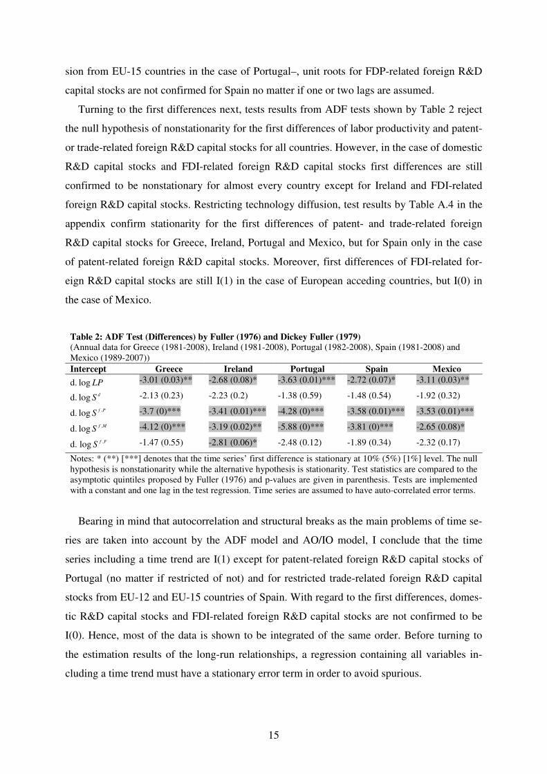
Turning to the first differences next, tests results from ADF tests shown by Table 2 reject

the null hypothesis of nonstationarity for the first differences of labor productivity and patent-

or trade-related foreign R&D capital stocks for all countries. However, in the case of domestic

R&D capital stocks and FDI-related foreign R&D capital stocks first differences are still

confirmed to be nonstationary for almost every country except for Ireland and FDI-related

foreign R&D capital stocks. Restricting technology diffusion, test results by Table A.4 in the

appendix confirm stationarity for the first differences of patent- and trade-related foreign

R&D capital stocks for Greece, Ireland, Portugal and Mexico, but for Spain only in the case

of patent-related foreign R&D capital stocks. Moreover, first differences of FDI-related for-

eign R&D capital stocks are still I(1) in the case of European acceding countries, but I(0) in

the case of Mexico.

Table 2: ADF Test (Differences) by Fuller (1976) and Dickey Fuller (1979) (Annual data for Greece (1981-2008), Ireland (1981-2008), Portugal (1982-2008), Spain (1981-2008) and Mexico (1989-2007))

Intercept Greece Ireland Portugal Spain Mexico

d. LPlog -3.01 (0.03)** -2.68 (0.08)* -3.63 (0.01)*** -2.72 (0.07)* -3.11 (0.03)**

d. dSlog -2.13 (0.23) -2.23 (0.2) -1.38 (0.59) -1.48 (0.54) -1.92 (0.32)

d. PfS

,log -3.7 (0)*** -3.41 (0.01)*** -4.28 (0)*** -3.58 (0.01)*** -3.53 (0.01)***

d. MfS

,log -4.12 (0)*** -3.19 (0.02)** -5.88 (0)*** -3.81 (0)*** -2.65 (0.08)*

d. FfS

,log -1.47 (0.55) -2.81 (0.06)* -2.48 (0.12) -1.89 (0.34) -2.32 (0.17)

Notes: * (**) [***] denotes that the time series’ first difference is stationary at 10% (5%) [1%] level. The null hypothesis is nonstationarity while the alternative hypothesis is stationarity. Test statistics are compared to the asymptotic quintiles proposed by Fuller (1976) and p-values are given in parenthesis. Tests are implemented with a constant and one lag in the test regression. Time series are assumed to have auto-correlated error terms.

Bearing in mind that autocorrelation and structural breaks as the main problems of time se-

ries are taken into account by the ADF model and AO/IO model, I conclude that the time

series including a time trend are I(1) except for patent-related foreign R&D capital stocks of

Portugal (no matter if restricted of not) and for restricted trade-related foreign R&D capital

stocks from EU-12 and EU-15 countries of Spain. With regard to the first differences, domes-

tic R&D capital stocks and FDI-related foreign R&D capital stocks are not confirmed to be

I(0). Hence, most of the data is shown to be integrated of the same order. Before turning to

the estimation results of the long-run relationships, a regression containing all variables in-

cluding a time trend must have a stationary error term in order to avoid spurious.

16

Cointegration Test: KPSS (1992)

Test results are based on the KPSS testing procedure and are compared to the asymptotic

quintiles at the 5% level proposed by Kwiatkowski, Phillips, Schmidt and Shin (1992). The

null hypothesis is that there is cointegration (i.e. residual is stationary), while the alternative

hypothesis is that there is no cointegration. As discussed, the KPSS testing procedures allows

for autocorrelation of the error term by introducing leads and lags of the first differences to

the test regression. By definition, the unit root equation for the estimated residuum from the

long-run relationship does not include a constant and a time trend. Tests have been conducted

for different technology diffusion channels (i.e. equation (3) in combination with patent-,

trade- and FDI-related diffusion channels by equations (5)-(7)). Table 3 shows test statistics

of the different model specifications if technology diffusion is unrestricted. In the case where

technology diffusion is restricted to EU-12 and EU-15 countries for European acceding coun-

tries and to the USA and Canada for Mexico, Table A.5 and Table A.6 in the appendix shows

test statistics respectively.

Starting with unrestricted technology diffusion, test statistics in Table 3 confirm the null

hypothesis of cointegration at a 5% level for almost every country and each model specifica-

tion except for Greece analyzing patent- and trade-related spillover effects and for Ireland

analyzing all three technology diffusion channels. Almost the same conclusion can be drawn

by the test statistics shown in Table A.5 in the appendix, where technology diffusion is re-

stricted to the EU-12 countries and to the USA accordingly. The only difference is that it is

Portugal, where the null hypothesis of cointegration is rejected in the case of all three tech-

nology diffusion channels. Allowing technology diffusion from EU-15 countries and from

USA and Canada, there is no cointegration for Greece in the case of patent- and trade related

spillover effects according to the test statistics shown by Table A.6 in the appendix.

Although all time series of the sample have been shown to be I(1) in levels, some have

failed to be I(0) in first differences reducing the cointegration analysis from above to those

time series with the same integrated order. Hence, to get a complete picture of the impact of

technology diffusion and economic integration on all integrating countries, estimates of the

long-run relationship between productivity and domestic and foreign R&D activity using

Engle and Granger (1987)’s two step EC model would lead to spurious results in cases where

stationary and nonstationary time series are combined. In case of doubt, the single equation

EC model is appropriate for both stationary and nonstationary data and provides information

about short term and long term effects on the equilibrium state. Therefore, it will be used as

17

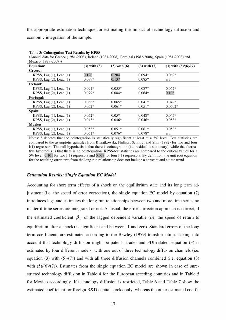
the appropriate estimation technique for estimating the impact of technology diffusion and

economic integration of the sample.

Table 3: Cointegation Test Results by KPSS


Equation: (3) with (5) (3) with (6) (3) with (7) (3) with (5)/(6)/(7)

Greece:

KPSS, Lag (1), Lead (1) 0.126 0.204 0.094* 0.062* KPSS, Lag (2), Lead (1) 0.099* 0.137 0.085* n.a.

Ireland:

KPSS, Lag (1), Lead (1) 0.091* 0.055* 0.087* 0.052* KPSS, Lag (2), Lead (1) 0.079* 0.084* 0.064* 0.108

Portugal:

KPSS, Lag (1), Lead (1) 0.068* 0.065* 0.041* 0.042* KPSS, Lag (2), Lead (1) 0.052* 0.061* 0.051* 0.0502*

Spain:


Mexico

KPSS, Lag (1), Lead (1) 0.053* 0.051* 0.061* 0.058* KPSS, Lag (2), Lead (1) 0.061* 0.076* 0.078* n.a.

Notes: * denotes that the cointegration is statistically significant at least at a 5% level. Test statistics are compared to the asymptotic quintiles from Kwiatkowski, Phillips, Schmidt and Shin (1992) for two and four I(1)-regressors. The null hypothesis is that there is cointegration (i.e. residual is stationary), while the alterna-tive hypothesis is that there is no cointegration. KPSS-test statistics are compared to the critical values for a 5% level: 0.101 for two I(1) regressors and 0.073 for four I(1) regressors. By definition, the unit root equation for the resulting error term from the long-run relationship does not include a constant and a time trend.

Estimation Results: Single Equation EC Model

Accounting for short term effects of a shock on the equilibrium state and its long term ad-

justment (i.e. the speed of error correction), the single equation EC model by equation (7)

introduces lags and estimates the long-run relationships between two and more time series no

matter if time series are integrated or not. As usual, the error correction approach is correct, if

the estimated coefficient i,1β of the lagged dependent variable (i.e. the speed of return to

equilibrium after a shock) is significant and between -1 and zero. Standard errors of the long

term coefficients are estimated according to the Bewley (1979) transformation. Taking into

account that technology diffusion might be patent-, trade- and FDI-related, equation (3) is

estimated by four different models: with one out of three technology diffusion channels (i.e.

equation (3) with (5)-(7)) and with all three diffusion channels combined (i.e. equation (3)

with (5)/(6)/(7)). Estimates from the single equation EC model are shown in case of unre-

stricted technology diffusion in Table 4 for the European acceding countries and in Table 5

for Mexico accordingly. If technology diffusion is restricted, Table 6 and Table 7 show the

estimated coefficient for foreign R&D capital stocks only, whereas the other estimated coeffi-

18

cients are postponed to the appendix and listed in Table A.7 and A.8 for the European coun-

tries and in A.9 for Mexico.

Patent-, trade and FDI-related spillover effects

Starting with unrestricted technology diffusion in the case of Greece, Ireland, Portugal and

Spain, the error correction approach is correct as the lagged coefficient of labor productivity is

significant and between -1 and zero for all countries except for Greece according to Table 4.

Ignoring therefore the estimation results of Greece, the coefficients of domestic R&D capital

stocks are significant at least at a 5% level for almost every country and each model specifica-

tion. Moreover, the signs are positive and fairly comparable to the results from Kao, Chiang

and Chen (1999) re-estimating Coe and Helpman (1995)’s paper and to Hafner (2008).5 While

both use panel data of OECD countries and dynamic OLS estimation techniques to estimate

the impact of foreign technology, the use of time series and single equation EC models lead to

higher coefficients of domestic R&D capital stocks for European acceding countries. As these

countries usually accounts for a certain degree of industrialization, they rely much more on

domestic R&D capital stocks than other (developing) OECD countries do. Turning to the

coefficient of foreign R&D capital stocks and therefore to technology diffusion, patent- and

trade-related spillover effects are significantly positive at least at a 5% level in the case of

Portugal for the first and Ireland for the second spillover effect if all four models are com-

pared. Hence, a 1% increase in R&D spending abroad raises labor productivity either between

0.02% and 0.05% in Portugal (i.e. equation (3) with (5) or with (5)/(6)/(7)) or between 0.19%

and 0.3% in Ireland (i.e. equation (3) with (6) or with (5)/(6)/(7)). With a focus of only one

single technology diffusion channel, patent-related spillover effects are significantly found for

Ireland with an impact of 0.02% on its labor productivity if foreign R&D capital stocks are

increased by 1%, whereas Spain’s labor productivity increases significantly from FDI-related

spillover effects by 0.04%.

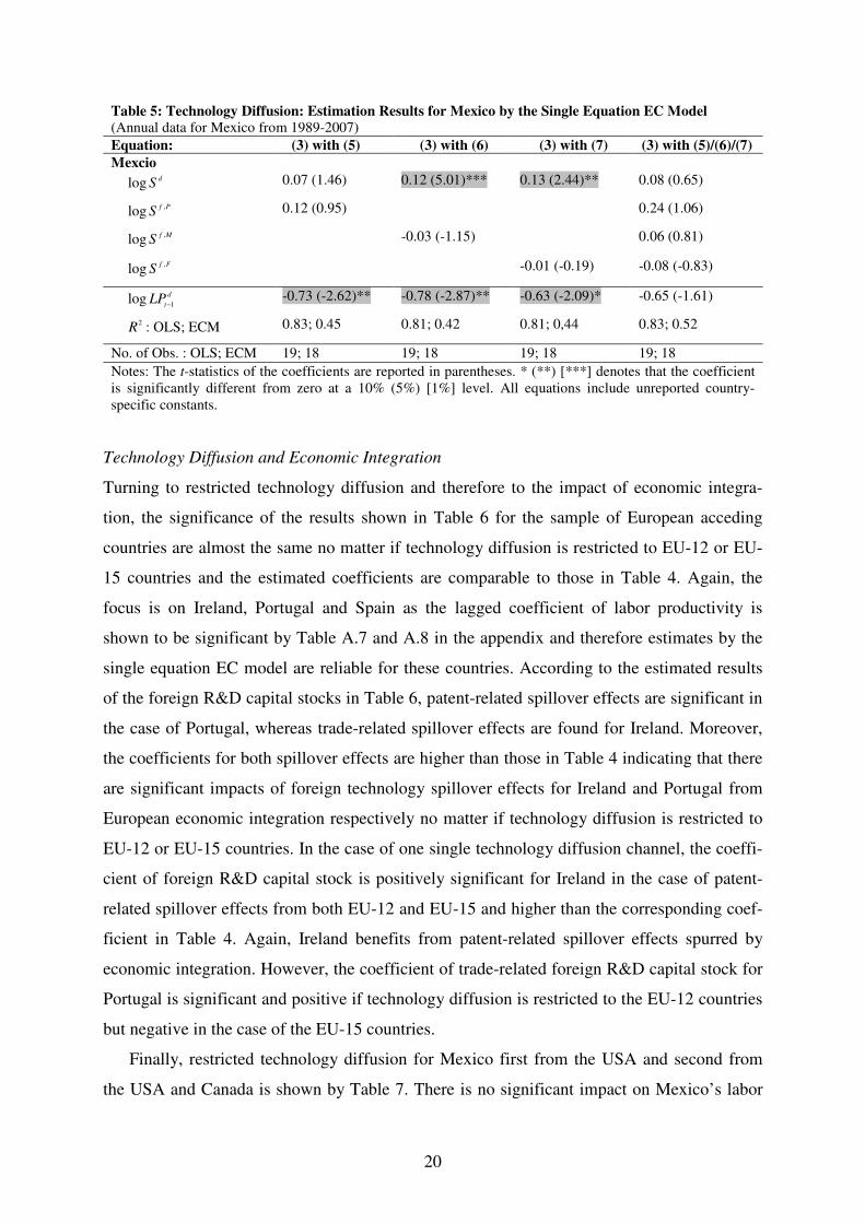
Estimation results for Mexico by Table 5 show that the error correction model is correct

for those models where one out of three technology diffusion channels are used. While there

is no empirical evidence for technology diffusion from abroad, the coefficient of domestic

R&D capital stocks is significantly positive but lower than in Table 4 – fairly comparable to

those from Kao, Chiang and Chen (1999) and Hafner (2008) as already discussed.

5 Both papers estimate the impact of domestic R&D capital stock amongst other variables. While Kao, Chiang and Chen (1999) estimates the impact on total factor productivity by 0.107, the coefficients in Hafner (2008) varies between 0.05 and 0.11 for Non-G7 OECD countries and between 0.128 and 0.144 for G7 countries.

19

Table 4: Technology Diffusion: Estimation Results for Greece, Ireland, Portugal and Spain by the

Single Equation EC Model (Annual data for Greece (1981-2008), Ireland (1981-2008), Portugal (1982-2008) and Spain (1981-2008))


Greece:

dSlog 0.31 (18.82)*** 0.45 (18.26)*** 0.49 (13.63)*** 0.49 (10.6)***

PfS

,log -0.01 (-1.73)* 0.03 (2.68)**

MfS

,log -0.48 (-8.04)*** 0.13 (1.44)

FfS

,log -0.93 (-5.74)*** -0.8 (-4.63)***

d

tLP

1log

− -0.1 (-0.71) -0.13 (-1.26) 0.13 (0.54) 0.24 (0.58)

2R : OLS; ECM 0.96; 0.10 0.92; 0.19 0.95; 0.32 0.95; 0.38

No. of Obs. : OLS; ECM 27; 26 27; 26 21; 20 21; 20

Ireland:

dSlog 0.38 (58.27)*** 0.33 (34.66)*** 0.36 (15.75)*** 0.35 (16.71)***

PfS

,log 0.02 (2.41)** -0.02 (-1.59)

MfS

,log 0.19 (4.06)*** 0.3 (3.64)**

FfS

,log 0 (0.05) -0.02 (-1.42)

d

tLP

1log

− -0.37 (-1.84)* -0.42 (-2.33)** -0.48 (-2.15)** -0.41 (-1.90)*

2R : OLS; ECM 1; 0.37 1; 0.48 1; 0.35 1; 0.57

No. of Obs. : OLS; ECM 28; 27 28; 27 26; 25 26; 25

Portugal:

dSlog 0.23 (24.31)*** 0.23 (25.31)*** 0.30 (7.34)** 0.42 (7.37)***

PfS

,log 0.02 (2.87)*** 0.05 (4.46)***

MfS

,log -0.29 (-4.05)*** -0.13 (-2.04)*

FfS

,log -0.02 (-1.52) -0.07 (-3.27)***

d

tLP

1log

− -0.42 (-2.52)** -0.23 (-1.88)* -0.33 (-2.70)*** -0.45 (-2.43)**

2R : OLS; ECM 0.94; 0.39 0.87; 0.41 0.91; 0,43 0.94; 055

No. of Obs. : OLS; ECM 27; 26 27; 26 27; 26 27; 26

Spain:

dSlog 0.10 (11.64)*** 0.19 (20.79)*** 0.04 (1.42) 0.2 (4.96)***

PfS

,log 0.01 (-1.80)* 0 (0.92)

MfS

,log -0.19 (-8.03)*** -0.2 (-6.03)***

FfS

,log 0.04 (3.07)*** 0 (0.01)

d

tLP

1log

− -0.23 (-2.86)*** -0.26 (-4.57)*** -0.25 (-4.07)*** -0.28 (-3.28)**

2R : OLS; ECM 0.96; 0.69 0.94; 0.75 0.94; 0.71 0.96; 0.75

No. of Obs. : OLS; ECM 28; 27 28; 27 28; 27 28; 27

Notes: The t-statistics of the coefficients are reported in parentheses. * (**) [***] denotes that the coefficient is significantly different from zero at a 10% (5%) [1%] level. All equations include unreported country-specific constants.

20

Table 5: Technology Diffusion: Estimation Results for Mexico by the Single Equation EC Model

(Annual data for Mexico from 1989-2007)


Mexcio

dSlog 0.07 (1.46) 0.12 (5.01)*** 0.13 (2.44)** 0.08 (0.65)

PfS

,log 0.12 (0.95) 0.24 (1.06)

MfS

,log -0.03 (-1.15) 0.06 (0.81)

FfS

,log -0.01 (-0.19) -0.08 (-0.83)

d

tLP

1log

− -0.73 (-2.62)** -0.78 (-2.87)** -0.63 (-2.09)* -0.65 (-1.61)

2R : OLS; ECM 0.83; 0.45 0.81; 0.42 0.81; 0,44 0.83; 0.52

No. of Obs. : OLS; ECM 19; 18 19; 18 19; 18 19; 18


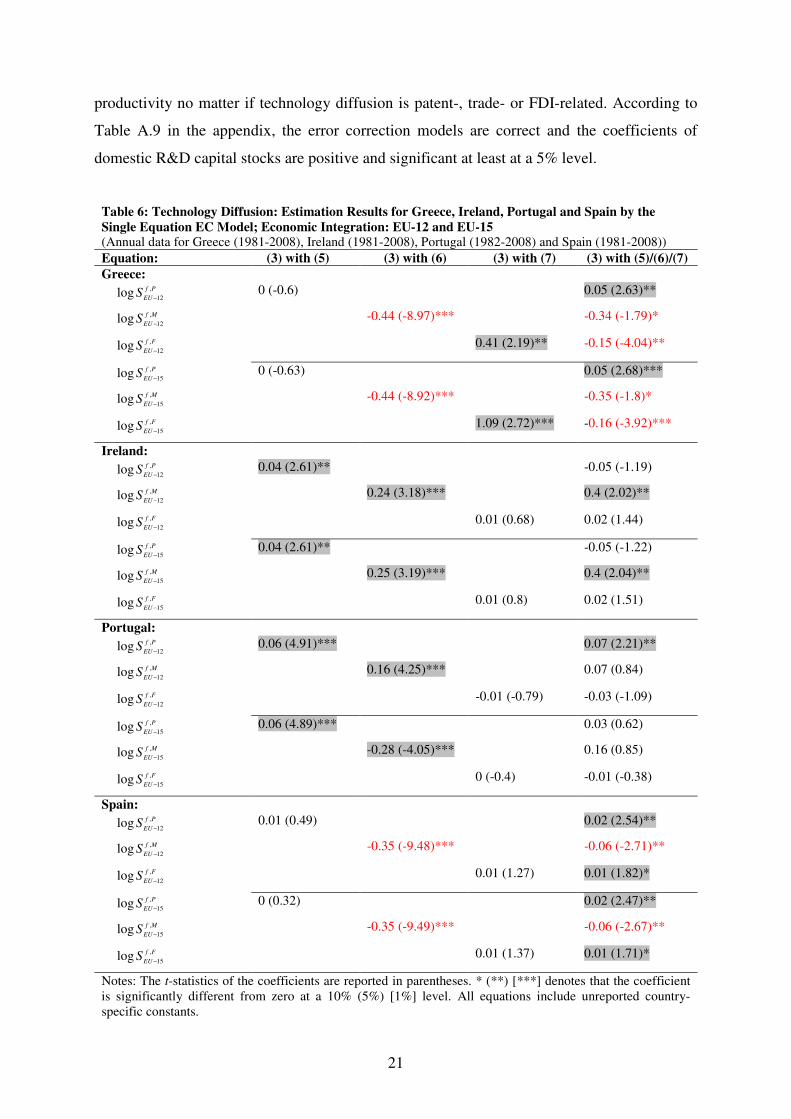
Technology Diffusion and Economic Integration

Turning to restricted technology diffusion and therefore to the impact of economic integra-

tion, the significance of the results shown in Table 6 for the sample of European acceding

countries are almost the same no matter if technology diffusion is restricted to EU-12 or EU-

15 countries and the estimated coefficients are comparable to those in Table 4. Again, the

focus is on Ireland, Portugal and Spain as the lagged coefficient of labor productivity is

shown to be significant by Table A.7 and A.8 in the appendix and therefore estimates by the

single equation EC model are reliable for these countries. According to the estimated results

of the foreign R&D capital stocks in Table 6, patent-related spillover effects are significant in

the case of Portugal, whereas trade-related spillover effects are found for Ireland. Moreover,

the coefficients for both spillover effects are higher than those in Table 4 indicating that there

are significant impacts of foreign technology spillover effects for Ireland and Portugal from

European economic integration respectively no matter if technology diffusion is restricted to

EU-12 or EU-15 countries. In the case of one single technology diffusion channel, the coeffi-

cient of foreign R&D capital stock is positively significant for Ireland in the case of patent-

related spillover effects from both EU-12 and EU-15 and higher than the corresponding coef-

ficient in Table 4. Again, Ireland benefits from patent-related spillover effects spurred by

economic integration. However, the coefficient of trade-related foreign R&D capital stock for

Portugal is significant and positive if technology diffusion is restricted to the EU-12 countries

but negative in the case of the EU-15 countries.

Finally, restricted technology diffusion for Mexico first from the USA and second from

the USA and Canada is shown by Table 7. There is no significant impact on Mexico’s labor

21

productivity no matter if technology diffusion is patent-, trade- or FDI-related. According to

Table A.9 in the appendix, the error correction models are correct and the coefficients of

domestic R&D capital stocks are positive and significant at least at a 5% level.

Table 6: Technology Diffusion: Estimation Results for Greece, Ireland, Portugal and Spain by the

Single Equation EC Model; Economic Integration: EU-12 and EU-15 (Annual data for Greece (1981-2008), Ireland (1981-2008), Portugal (1982-2008) and Spain (1981-2008))


Greece:

Pf

EUS ,

12log

− 0 (-0.6) 0.05 (2.63)**

Mf

EUS ,

12log

− -0.44 (-8.97)*** -0.34 (-1.79)*

Ff

EUS ,

12log

− 0.41 (2.19)** -0.15 (-4.04)**

Pf

EUS ,

15log

− 0 (-0.63) 0.05 (2.68)***

Mf

EUS ,

15log

− -0.44 (-8.92)*** -0.35 (-1.8)*

Ff

EUS ,

15log

− 1.09 (2.72)*** -0.16 (-3.92)***

Ireland:

Pf

EUS ,

12log

− 0.04 (2.61)** -0.05 (-1.19)

Mf

EUS ,

12log

− 0.24 (3.18)*** 0.4 (2.02)**

Ff

EUS ,

12log

− 0.01 (0.68) 0.02 (1.44)

Pf

EUS ,

15log

− 0.04 (2.61)** -0.05 (-1.22)

Mf

EUS ,

15log

− 0.25 (3.19)*** 0.4 (2.04)**

Ff

EUS ,

15log

− 0.01 (0.8) 0.02 (1.51)

Portugal:

Pf

EUS ,

12log

− 0.06 (4.91)*** 0.07 (2.21)**

Mf

EUS ,

12log

− 0.16 (4.25)*** 0.07 (0.84)

Ff

EUS ,

12log

− -0.01 (-0.79) -0.03 (-1.09)

Pf

EUS ,

15log

− 0.06 (4.89)*** 0.03 (0.62)

Mf

EUS ,

15log

− -0.28 (-4.05)*** 0.16 (0.85)

Ff

EUS ,

15log

− 0 (-0.4) -0.01 (-0.38)

Spain:

Pf

EUS ,

12log

− 0.01 (0.49) 0.02 (2.54)**

Mf

EUS ,

12log

− -0.35 (-9.48)*** -0.06 (-2.71)**

Ff

EUS ,

12log

− 0.01 (1.27) 0.01 (1.82)*

Pf

EUS ,

15log

− 0 (0.32) 0.02 (2.47)**

Mf

EUS ,

15log

− -0.35 (-9.49)*** -0.06 (-2.67)**

Ff

EUS ,

15log

− 0.01 (1.37) 0.01 (1.71)*


22

Table 7: Technology Diffusion: Estimation Results for Mexico by the Single Equation EC Model;

Economic Integration: USA and USA/CAN



Mexico:

Pf

USAS ,log 0.08 (0.7) 0.23 (1.07)

Mf

USAS ,log -0.02 (-1.1) 0.06 (0.86)

Ff

USAS ,log -0.04 (-1.32) -0.09 (-1.08)

Pf

CANUSAS ,

/log 0.08 (0.7) 0.23 (1.04)

Mf

CANUSAS ,

/log -0.02 (-1.1) 0.06 (0.86)

Ff

CANUSAS ,

/log -0.04 (-1.28) -0.09 (-1.07)


To sum up, the paper finds empirical evidence for foreign technology spillover effects. For-

eign R&D capital stocks are trade-related in the case of Ireland, patent-related in the case of

Portugal and FDI-related in the case of Spain. Moreover, there are significant impacts of

foreign technology spillover effects for Ireland and Portugal from European economic inte-

gration no matter if technology diffusion is restricted to EU-12 or EU-15 countries, whereas

in the case of Mexico no such evidence from joining NAFTA is found.

7 Conclusions

Research activity and its technological spillover effects are widely believed to be crucial for

structural backward countries within economically integrating regions. In such regions, coun-

tries compete not only for manufacturing activities but also for mobile factors such as skilled

labor and capital. Moreover, further economic integration according to Hafner (2011) spur

technology diffusion through tighter relationships. However, such technology diffusion and

the adoption of foreign technological knowledge may have different impacts on countries.

While for industrialized countries technology diffusion towards integrating countries may

result in a loss of industry shares and mobile factors, structurally backward countries certainly

gain by technology diffusion especially those with low domestic R&D spending. Hence, it

turns out to be essential for structurally backward countries to gain access to technological

knowledge to increase industrial activity and upgrade local industries. A better access to

foreign R&D knowledge improves the possibilities to close the gap toward the technological

frontier and to participate in world markets.

23

Is it all about investing in R&D and foreign technology spillover effects? Returning to the

empirical results, the answer is definitely yes at least for the European countries. In addition

to the significant impacts of domestic R&D spending on labor productivity, there is empirical

evidence for foreign technology spillover effects for Ireland, Portugal and Spain, but not for

Greece, where estimation results are spurious and therefore have been ignored. Patent-related

spillover effects are found for Portugal and Ireland such that a 1% increase in R&D spending

abroad raises labor productivity between 0.02% and 0.05% in Portugal and 0.02% in Ireland.

Moreover, there is empirical evidence for trade-related spillover effects for Ireland estimated

between 0.19% and 0.3% and for FDI-related spillover effects for Spain estimated by 0.04%

respectively. Comparing the estimated results of foreign technology spillover effects in cases

of unrestricted and restricted technology diffusion, the paper finds significant impacts from

European economic integration. In particular, Portugal and Ireland benefit most from joining

the EU as coefficients are higher for patent- and trade-related spillover effects in the case of

restricted technology diffusion from EU-12 or EU-15 countries. Turning to Mexico, there is

no significant impact on Mexico’s labor productivity no matter if technology diffusion is

patent-, trade- or FDI-related. Moreover, there is no evidence that joining the free trade

agreement with the USA and Canada has a significant positive effect. According to the analy-

sis, it is only domestic R&D spending which has a major significant impact on labor produc-

tivity in Mexico.

24

References

Banerjee, A., Dolado, J.J., Mestre, R., 1998. Error-correction mechanism tests for

cointegration in a single-equation framework, Journal of Time Series Analysis 19, 267-

283.

Baum, C.F., 2005. Stata: The language of choice for time-series analysis?, The Stata Journal

5, 46-63.

Bewley, R., 1979. The direct estimation of the equilibrium response in a linear dynamic mod-

el, Economics Letters 3, 357-361.

Biswal, B., Dhawan, U., 1998. Export-led growth hypothesis: cointegration and causality

analysis for Taiwan, Applied Economics Letters 5, 699–701.

Branstetter, L., 2005. Is foreign direct investment a channel of knowledge spillover? Evidence

from Japan’s FDI in the United States, Journal of International Economics 68, 325-344.

Branstetter, L., Sakakibara, M., 2001. Do stronger patents induce more innovation? Evidence

from the 1988 Japanese patent law reforms. RAND Journal of Economics 32, 77–100.

Ghatak, S., Milner, C., Utkulu, U., 1997. Exports, export composition and growth: cointegra-

tion and causality evidence for Malaysia, Applied Economics 29, 213–223.

Cabral, R., Mollick, A.V., 2011. Intra-industry trade effects on Mexican manufacturing

productivity before and after NAFTA, The Journal of International Trade & Economic

Development 20, 87-112.

Clemente, J., Montañés, A., Reyes, M., 1998. Testing for a unit root in variables with a dou-

ble change in the mean, Economics Letters 59, 175-182.

Coe, D.T., Helpman, E., 1995. International R&D spillovers, European Economic Review 39,

859–887.

Dickey, D.A., Fuller, W.A., 1979. Distribution of the estimators for autoregressive time series

with a unit root, Journal of the American Statistical Association 74, 427–431.

Eaton, J., Kortum, S., 1999. International technology diffusion: theory and measurement,

International Economic Review 40, 537–570.

Engle, R.F., Granger, C.W.J., 1987. Co-integration and error correction: representation, esti-

mation, and testing, Econometrica 55, 12-26.

Fuller, W., 1976. Introduction to Statistical Time Series, Wiley New York, NY.

Griliches, Z., 1979. Issues in assessing the contribution of R&D to productivity growth, Bell

Journal of Economics 10, 92–116.

25

GGDC, 2010. Total Economy Database, Groningen Growth and Development Center, Gro-

ningen.

Hafner, K.A., 2008. The pattern of international patenting and technology diffusion, Applied

Economics 40, 2819-2837.

Hafner, K.A., 2011. Trade liberalization and technology diffusion, Review of International

Economics 19, 963-978.

Haskel, J., Pereira, S., Slaughter, M., 2007. Does inward foreign direct investment boost the

productivity of domestic firms?, The Review of Economics and Statistics 89, 482-496.

Hassler, U., Wolters, J., 2006. Autoregressive distributed lag models and cointegration, AStA

Advances in Statistical Analysis 90, 59-74.

Hufbauer, G., Schott, J., 1993. NAFTA: An Assessment. Washington DC: Institute for Interna-

tional Economics.

Jaffe, A.B., Trajtenberg, M., 2002. Patents, Citations, and Innovations: A window on the

Knowledge Economy, MIT Press, Cambrigde, MA.

Khalifah, N.A., Adam, R., 2009. Productivity spillovers from FDI in Malaysian manufactur-

ing: evidence from micro-panel data, Asian Economic Journal 23, 143-167.

Kao, C., Chiang, M.-H., Chen, B., 1999. International R&D spillovers: an application of

estimation and inference in panel cointegration, Oxford Bulletin of Economics and Sta-

tistics 61, 691–709.

Keller, W., 2004. International technology diffusion, Journal of Economic Literature 42,

752–782.

Keller, W., Yeaple, S.R., 2009. Multinational enterprises, international trade, and productivity

growth: firm-level evidence from the United States. The Review of Economics and Sta-

tistics 91, 821-831.

Kleinert, J., Toubal, F., 2010. Gravity for FDI, Review of International Economics 18, 1-13.

Kramer, S.M.S., 2010. International R&D spillovers in emerging markets: the impact of trade

and foreign direct investment, The Journal of International Trade & Economic Devel-

opement 19, 591-623.

Kwiatkowski, D., Phillips, P.C.B, Schmidt, P., Shin, Y., 1992. Testing the null hypothesis of

stationarity against the alternative of a unit root, Journal of Econometrics 54, 159-178.

MacKinnon, J.G., 1991. Critical values for cointegration tests, in R.F. Engle and C.W.J.

Granger (eds.), Long-run Economic Relationships: Readings in Cointegration, Oxford

University Press, Oxford.

26

OECD, 2011. Economic Outlook Database, Organisation of Economic Co-operation and

Development, Paris.

–, 2009. International Direct Investment Statistics, Organisation of Economic Co-operation

and Development, Paris.

–. 2010a. Main Science and Technology Database, Organisation of Economic Co-operation


–. 2010b. Monthly Statistics of International Trade, Organisation of Economic Co-operation


Perron, P., Vogelsang, T., 1992. Nonstationarity and level shifts with an application to pur-

chasing power parity, Journal of Business and Economic Statistics 10, 301-320.

Savvides, A., Zachariadis, M., 2005. International technology diffusion and the growth of

TFP in the manufacturing sector of developing economies, Review of Development

Economies 9, 482-501.

Unel, B., 2010. Technology diffusion trough trade with heterogeneous firms, Review of Inter-

national Economics 18, 465-481.

WIPO, 2001. Industrial Property Statistics Publication B Part I. World Intellectual Property

Organization, Geneva.

–, 2009. Statistic Database. World Intellectual Property Organization, Geneva.

Wolters, J., Kirchgaessner, G., 2008. Introduction to Modern Time Series Analysis, Springer

Verlag, Berlin.

Xu, B., Chiang, E.P., 2005. Trade, patents and international technology diffusion, The Journal

of International Trade & Economic Development 14, 114-135.

27

Appendix

Table A.1: R&D Capital Stock Data

(BERD Expenditure in million constant US$ (PPP))

R&D Expenditure R&D Capital Stocks

Period Flow Annual Growth Depreciation Year Benchmark

Greece 1981-2007 50.5 8.1424 0.1 1981 278.6

Ireland 1981-2008 115.9 9.3872 0.1 1981 597.8

Portugal 1982-2008 87.3 10.8971 0.1 1982 417.6

Spain 1981-2007 887.6 8.2284 0.1 1981 4,869.6

Mexico 1989-2007 466.1 8.2099 0.1 1989 2,559.5

Notes: The benchmark is calculated following the procedure suggested by Griliches (1979). Depreciation rate is assumed to be 10%. Annual growth rates (%) are calculated according to the time period.

Table A.2: FDI Inflow Stock Data

(FDI Inflow in million current US$)

FDI Inflow FDI Stock

Total World Period Flow Annual Growth Depreciation Year Benchmark

Greece 1987-2007 1,258.1 2.0430 0.1 1987 10,446.8

Ireland 1983-2007 237.5 21.4508 0.1 1983 755.1

Portugal 1981-2007 139.0 14.6951 0.1 1981 562.9

Spain 1981-2007 851.9 16.9036 0.1 1981 3,166.5

Mexico 1989-2007 3,881.5 7.7889 0.1 1989 21,819.7

EU-12; USA

Greece 1987-2008 597.3 8.959 0.1 1987 3,161.1

Ireland 1985-2008 71.2 15.7006 0.1 1985 276.9

Portugal 1985-2008 111.0 14.7756 0.1 1985 448.0

Spain 1985-2008 641.7 21.4699 0.1 1985 2,039.2

Mexico 1985-2008 1.942,5 7.5077 0.1 1985 11,095.1

EU-15; USA-CAN

Greece 1987-2008 641.8 8.4872 0.1 1987 3,471.6

Ireland 1985-2008 75.3 20.1588 0.1 1985 249.5

Portugal 1985-2008 114.0 15.2643 0.1 1985 451.2

Spain 1985-2008 670.4 21.3488 0.1 1985 2,138.5

Mexico 1985-2008 2,039.8 8.3869 0.1 1985 11,093.7

Notes: The benchmark is calculated following the procedure suggested by Griliches (1979). Depreciation rate is assumed to be 10%. Annual growth rates (%) are calculated according to the time period.

28

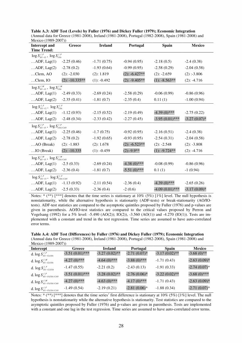
Table A.3: ADF Test (Levels) by Fuller (1976) and Dickey Fuller (1979); Economic Integration


Intercept and

Time Trend:

Greece Ireland Portugal Spain Mexico

Pf

EUS ,

12log

−, Pf

USAS ,log

…ADF, Lag(1) -2.25 (0.46) -1.71 (0.75) -0.94 (0.95) -2.18 (0.5) -2.4 (0.38)

…ADF, Lag(2) -2.78 (0.2) -1.93 (0.64) -0.99 (0.95) -2.58 (0.29) -2.04 (0.58)

…Clem, AO (2): -2.030 (2): 1.819 (2): -6.427** (2): -2.659 (2) :-3.806

…Clem, IO (2): -10.335** (1): -0.492 (2): -9.405** (1): -8.563** (2): -4.716

Mf

EUS ,

12log

−, Mf

USAS ,log

…ADF, Lag(1) -2.49 (0.33) -2.69 (0.24) -2.58 (0.29) -0.06 (0.99) -0.86 (0.96)

…ADF, Lag(2) -2.35 (0.41) -1.81 (0.7) -2.35 (0.4) 0.11 (1) -1.00 (0.94)

Ff

EUS ,

12log

−, Ff

USAS ,log

…ADF, Lag(1) -1.12 (0.93) -2.15 (0.52) -2.19 (0.49) -4.39 (0)*** -2.75 (0.22)

…ADF, Lag(2) -2.48 (0.34) -2.33 (0.42) -2.27 (0.45) -3.95 (0.01)*** -3.27 (0.07)*

Pf

EUS ,

15log

−, Pf

CANUSAS ,

/log

…ADF, Lag(1) -2.25 (0.46) -1.7 (0.75) -0.92 (0.95) -2.16 (0.51) -2.4 (0.38)

…ADF, Lag(2) -2.78 (0.2) -1.92 (0.65) -0.93 (0.95) -2.54 (0.31) -2.04 (0.58)

…AO (Break) (2): -1.883 (2): 1.678 (2): -6.523** (2): -2.548 (2): -3.808

…IO (Break) (2): -10.335 (1): -0.459 (2):-9.9** (1): -9.724** (2): -4.716

Mf

EUS ,

15log

−, Mf

CANUSAS ,

/log

…ADF, Lag(1) -2.5 (0.33) -2.69 (0.24) -4.38 (0)*** -0.08 (0.99) -0.86 (0.96)

…ADF, Lag(2) -2.36 (0.4) -1.81 (0.7) -5.51 (0)*** 0.1 (1) -1 (0.94)

Ff

EUS ,

15log

−, Ff

CANUSAS ,

/log

…ADF, Lag(1) -1.13 (0.92) -2.11 (0.54) -2.36 (0.4) -4.39 (0)*** -2.65 (0.26)

…ADF, Lag(2) -2.5 (0.33) -2.36 (0.4) -2 (0.6) -4.09 (0.01)*** -3.17 (0.09)*

Notes: * (**) [***] denotes that the time series is stationary at 10% (5%) [1%] level. The null hypothesis is nonstationarity, while the alternative hypothesis is stationarity (ADF-tests) or break-stationarity (AO/IO-tests). ADF-test statistics are compared to the asymptotic quintiles proposed by Fuller (1976) and p-values are given in parenthesis. AO/IO-test statistics are compared to the critical values proposed by Perron and Vogelsang (1992) for a 5% level: -5.490 (AO(2)); IO(2)), -3.560 (AO(1)) and -4.270 (IO(1)). Tests are im-plemented with a constant and trend in the test regression. Time series are assumed to have auto-correlated error terms.

Table A.4: ADF Test (Differences) by Fuller (1976) and Dickey Fuller (1979); Economic Integration


Intercept Greece Ireland Portugal Spain Mexico

d. Pf

USAEUS

,

;12log

− -3.51 (0.01)*** -3.27 (0.02)** -2.71 (0.07)* -3.17 (0.02)** -3.68 (0)**

d. Mf

USAEUS

,

;12log

− -4.27 (0)*** -4.64 (0)*** -3.88 (0)*** -1.71 (0.43) -2.63 (0.09)*

d. Ff

USAEUS

,

;12log

− -1.47 (0.55) -2.21 (0.2) -2.43 (0.13) -1.91 (0.33) -2.74 (0.07)*

d. Pf

CANUSAEUS

,

/;15log

− -3.51 (0.01)*** -3.28 (0.02)** -2.76 (0.06)* -3.22 (0.02)** -3.68 (0)***

d. Mf

CANUSAEUS

,

/;15log

− -4.27 (0)*** -4.63 (0)*** -4.17 (0)*** -1.71 (0.43) -2.63 (0.09)*

d. Ff

CANUSAEUS

,

/;15log

− -1.49 (0.54) -2.19 (0.21) -2.81 (0.06)* -1.88 (0.34) -2.71 (0.07)*

Notes: * (**) [***] denotes that the time series’ first difference is stationary at 10% (5%) [1%] level. The null hypothesis is nonstationarity while the alternative hypothesis is stationarity. Test statistics are compared to the asymptotic quintiles proposed by Fuller (1976) and p-values are given in parenthesis. Tests are implemented with a constant and one lag in the test regression. Time series are assumed to have auto-correlated error terms.

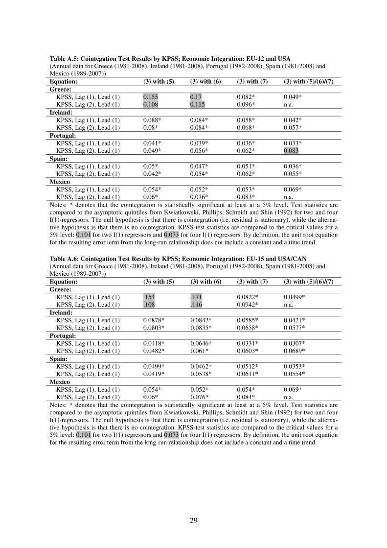
29

Table A.5: Cointegation Test Results by KPSS; Economic Integration: EU-12 and USA



Greece:

KPSS, Lag (1), Lead (1) 0.155 0.17 0.082* 0.049* KPSS, Lag (2), Lead (1) 0.108 0.115 0.096* n.a.

Ireland:


Portugal:

KPSS, Lag (1), Lead (1) 0.041* 0.039* 0.036* 0.033* KPSS, Lag (2), Lead (1) 0.049* 0.056* 0.062* 0.083

Spain:


Mexico



Table A.6: Cointegation Test Results by KPSS; Economic Integration: EU-15 and USA/CAN



Greece:

KPSS, Lag (1), Lead (1) .154 .171 0.0822* 0.0499* KPSS, Lag (2), Lead (1) .108 .116 0.0942* n.a.

Ireland:


Portugal:


Spain:


Mexico



30

Table A.7: Technology Diffusion: Estimation Results for Greece, Ireland, Portugal and Spain by the

Single Equation EC Model; Economic Integration: EU-12 (Annual data for Greece (1981-2008), Ireland (1981-2008), Portugal (1982-2008) and Spain (1981-2008))


Greece:

dSlog 0.33 (18.64)*** 0.36 (23.87)*** 0.05 (0.41) 0.48 (12.69)***

d

tLP 1log − -0.08 (-0.64) -0.2 (-1.71)* -0.06 (-0.2) -0.44 (-1.08)

2R : OLS; ECM 0.95; 0.12 0.94; 0.22 0.96; 0.24 0.97; 0.47

No. of Obs. : OLS; ECM 27; 26 27; 26 21; 20 21; 20

Ireland:

dSlog 0.38 (56.49)*** 0.37 (79.56)*** 0.35 (18.05)*** 0.31 (10.47)***

d

tLP 1log − -0.39 (-2.02)** -0.37 (-1.84)* -0.45 (-1.83)* -0.41 (-1.51)

2R : OLS; ECM 1; 0.4 1; 0.4 0.99; 0.35 1; 0.47

No. of Obs. : OLS; ECM 28; 27 28; 27 24; 23 24; 23

Portugal:

FfS

,log -0.01 (-0.79) -0.03 (-1.09)

d

tLP 1log − -0.5 (-3.2)*** -0.44 (-2.63)*** -0.33 (-2.4)** -0.53 (-1.89)*

2R : OLS; ECM 0.94; 0.44 0.95; 0.46 0.89; 0.38 0.94; 0.45

No. of Obs. : OLS; ECM 27; 26 27; 26 24; 23 24; 23

Spain:

FfS

,log 0.01 (1.27) 0.01 (1.82)*

d

tLP 1log − -0.26 (-3.12)*** -0.13 (-1.92)* -0.67 (-3.69)*** -0.58 (-3.32)***

2R : OLS; ECM 0.96; 0.69 0.96; 0.77 0.97; 0.59 0.97; 0.79

No. of Obs. : OLS; ECM 28; 27 28; 27 24; 23 24; 23


Table A.8: Technology Diffusion: Estimation Results for Greece, Ireland, Portugal and Spain by the

Single Equation EC Model; Economic Integration: EU-15

(Annual data for Greece (1981-2008), Ireland (1981-2008), Portugal (1982-2008) and Spain (1981-2008))


Greece:

dSlog 0.33 (18.66)*** 0.36 (23.58)*** -0.34 (-1.42) 0.49 (12.41)***

d

tLP 1log − -0.08 (-0.64) -0.2 (-1.7)* -0.03 (-0.1) -0.43 (-1.03)

2R : OLS; ECM 0.95; 0.12 0.94; 0.21 0.96; 0.25 0.97; 0.46

No. of Obs. : OLS; ECM 27; 26 27; 26 21; 20 21; 20

Ireland:

dSlog 0.38 (56.9)*** 0.37 (79.49)*** 0.35 (17.44)*** 0.31 (10.35)***

d

tLP 1log − -0.39 (-2.02)** -0.37 (-1.84)* -0.45 (-1.84)* -0.41 (-1.51)

2R : OLS; ECM 1; 0.4 1; 0.4 0.99; 0.35 1; 0.47

No. of Obs. : OLS; ECM 28; 27 28; 27 24; 23 24; 23

Portugal:

dSlog 0.26 (21.59)*** 0.23 (25.31)*** 0.2 (5.99)*** 0.23 (1.55)

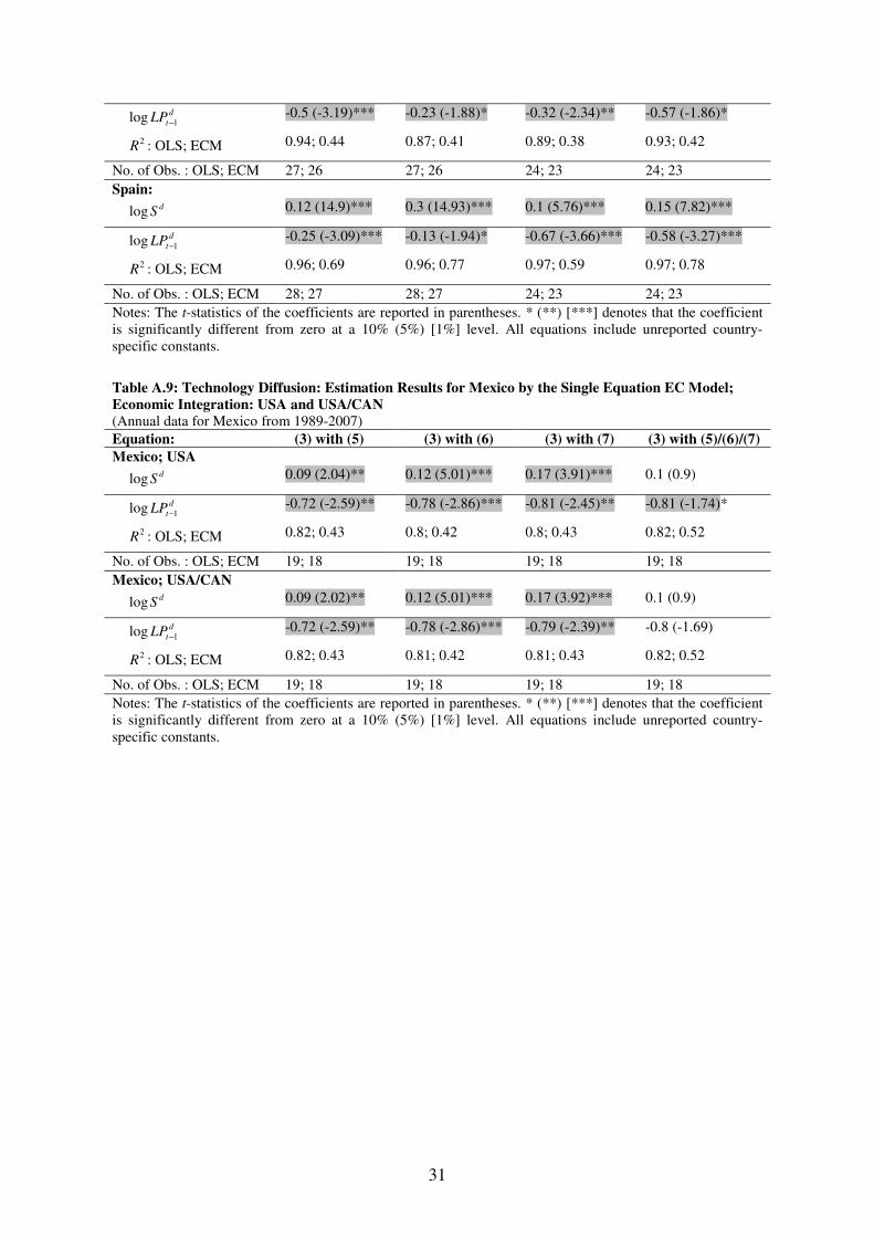
31

d

tLP 1log − -0.5 (-3.19)*** -0.23 (-1.88)* -0.32 (-2.34)** -0.57 (-1.86)*

2R : OLS; ECM 0.94; 0.44 0.87; 0.41 0.89; 0.38 0.93; 0.42

No. of Obs. : OLS; ECM 27; 26 27; 26 24; 23 24; 23

Spain:

dSlog 0.12 (14.9)*** 0.3 (14.93)*** 0.1 (5.76)*** 0.15 (7.82)***

d

tLP 1log − -0.25 (-3.09)*** -0.13 (-1.94)* -0.67 (-3.66)*** -0.58 (-3.27)***

2R : OLS; ECM 0.96; 0.69 0.96; 0.77 0.97; 0.59 0.97; 0.78

No. of Obs. : OLS; ECM 28; 27 28; 27 24; 23 24; 23


Table A.9: Technology Diffusion: Estimation Results for Mexico by the Single Equation EC Model;

Economic Integration: USA and USA/CAN



Mexico; USA

dSlog 0.09 (2.04)** 0.12 (5.01)*** 0.17 (3.91)*** 0.1 (0.9)

d

tLP 1log − -0.72 (-2.59)** -0.78 (-2.86)*** -0.81 (-2.45)** -0.81 (-1.74)*

2R : OLS; ECM 0.82; 0.43 0.8; 0.42 0.8; 0.43 0.82; 0.52

No. of Obs. : OLS; ECM 19; 18 19; 18 19; 18 19; 18

Mexico; USA/CAN

dSlog 0.09 (2.02)** 0.12 (5.01)*** 0.17 (3.92)*** 0.1 (0.9)

d

tLP 1log − -0.72 (-2.59)** -0.78 (-2.86)*** -0.79 (-2.39)** -0.8 (-1.69)

2R : OLS; ECM 0.82; 0.43 0.81; 0.42 0.81; 0.43 0.82; 0.52

No. of Obs. : OLS; ECM 19; 18 19; 18 19; 18 19; 18


Technology Spillover Effects and Economic Integration -...

Documents

Transcript of Technology Spillover Effects and Economic Integration -...