Technology Ladders and R&D in Dynamic Cournot Markets

Mike Ludkovski∗ Ronnie Sircar†

June 2015, revised November 16, 2015

Abstract

Motivated by dramatic and unpredictable technological advances in energy production (forinstance drilling and extraction of shale oil), we extend Cournot models of competition toincorporate research and development (R&D) that can lead to (stochastic) drops in productioncosts. Our model combines features of patent racing with dynamic market structure, capturingthe interplay between the immediate competition in terms of production rates and the long-termcompetition in R&D. The resulting Markov Nash equilibrium is found from a sequence of one-step static games arising between R&D successes, and several numerical examples and extensiveanalysis of the emerging comparative statics are presented. Analyzing the relationship betweencurrent market dominance and the level of R&D investments, we find that market leaderstend to invest more, which in some sense makes oligopoly dynamically unstable. We showthat anticipated market transitions have long-term impact; for example the potential of futuremonopoly can spur R&D investment now, even if the firm is presently uncompetitive and notactively producing. We also show that, surprisingly, random innovations have an ambiguouseffect on R&D. This feature, which is driven by the Cournot framework, contrasts with thecommon situation whereby uncertainty lowers innovation and delays R&D investments. Finally,we demonstrate that increased competition may actually increase efforts to innovate throughhigher desire to achieve dominance. This would match the anecdotal evidence that the threatof market entrants forces incumbents to maintain high R&D.

Keywords: Cournot markets, R&D innovations, technology ladder, dynamic oligopolyJEL Codes: D43, O32, C73, L13

1 Introduction

In the past decade, major advances in deep-sea offshore oil, tanker technology, and especially shaleoil have fundamentally altered the oil market, marginalizing traditional producers and elevating newplayers. These effects can be ascribed to dramatically lower production costs of these technologies.A recent article in the New York Times quotes that “the break-even price for operating in 75percent of the shale oil fields a year ago was $75 a barrel, but that is now down to roughly $60because of innovation and lower service company costs... the break-even cost could go as low as$50 before long.” [Krauss, 2015] The alluded innovations are uncertain and unpredictable – witness

∗Department of Statistics and Applied Probability, University of California Santa Barbara, South Hall, SantaBarbara, CA 93106-3110; ludkovski@pstat.ucsb.edu. We thank Mark Duggan for research assistance, Rene Aid andHans Tuenter for helpful discussions. We also thank participants at the Banff Workshop on New Directions inFinancial Mathematics and Mathematical Economics (July 2014) and IPAM Workshop on Commodity Markets andtheir Financialization (May 2015) for their feedback.†ORFE Department, Princeton University, Sherrerd Hall, Princeton, NJ, 08544; sircar@princeton.edu. Work

partially supported by NSF grant DMS-1211906.

1

the disruptive power of shale production which was a sudden development unanticipated even 15years ago. Conversely, consider the story of arctic oil production which remains minimal even afterdecades of exploration due to unforeseen challenges. Moreover, technical progress is not a one-timeevent, but a series of changes representing accumulation of knowledge stock and correspondingtechnology advances, all requiring sustained investments in research and development.

Motivated by these economic realities, in this paper we investigate dynamic stochastic Research& Development (R&D) games. The underlying framework of a non-cooperative oligopoly is apopular tool for describing commodity market equilibrium and is to be understood broadly, forexample via various producer types in the oil market (conventional sweet crude, offshore oil, oilsands, shale oil, etc.) The dynamic aspect arises due to the two time scales for competitionbetween producers. In the short term, firms compete on quantity, interacting through the aggregatesupply-demand equilibrium. In the long term, firms also compete on innovation through generatingstructural competitive advantages. As described above for the crude oil market, one way to gainadvantage is to improve efficiency through lower extraction costs.

To capture game effects which are present on both time scales we consider a Cournot marketmodel with the producers endogenously improving their production costs. More precisely, wedescribe technological advances as a controlled point process, where the timing of innovation eventsis influenced by the investment in R&D. Consequently, progress is stochastically dependent on theresearch effort but is totally unpredictable otherwise. Innovation gains are assumed to be permanentand private, generating a durable competitive advantage to the innovator. The discrete nature ofinnovation implies that the market evolves through a sequence of technology stages. This setup alsodecouples the instantaneous equilibrium, equivalent to a static Cournot game, from the long-termcost competition that is described through dynamic-programming-type recursions.

1.1 Contributions

Our dynamic R&D game provides a link between models of stochastic innovation/patent races andof Cournot markets. Integrating both aspects in a single game theoretic framework gives insightsinto the interplay between joint optimization of production and R&D. Notably, the developed modelendogenizes the market structure, making the number of active producers time-varying, so as toallow an endogenous transition between, say, duopoly and monopoly. Thus, we are able to capturethe aforementioned history of oil production whereby some technologies dynamically enter andleave the market (e.g. the recent entry of shale production and the resulting effective suspensionof deep-sea exploration). Endogenous market structure is only possible in a multi-stage setup andhighlights the dynamism of our framework.

Our analysis yields several novel insights and features. First, we analyze the relationship be-tween current market dominance and the level of R&D investments. We find that market leaderstend to invest more, which in some sense makes oligopoly dynamically unstable. Second, we showthat anticipated market transitions have long-term impact; for example the potential of futuremonopoly can spur R&D investment now, even if the firm is presently uncompetitive and not ac-tively producing. Third, we provide results and extensive discussion on the role of stochasticityin R&D. The fact that innovations are fundamentally uncertain in our model implies that there isalways a range of scenarios for the future competition conditions. Surprisingly we show that ran-dom innovations have an ambiguous effect on R&D. This feature, which is driven by the Cournotframework, contrasts with the common situation whereby uncertainty lowers innovation and delaysR&D investments. Fourth, we investigate the role of competition in R&D. We demonstrate thatincreased competition may actually increase efforts to innovate through higher desire to achievedominance. This would match the anecdotal evidence that the threat of market entrants forcesincumbents to maintain high R&D.

2

On the modeling front, our setup is mathematically tractable, directly building on top of theclassical theory of Cournot competition. As such, we are able to use insights from static games toshed light on features of the dynamic model. In particular, we analyze the relationship between thestatic dependence of profits on costs and the dynamic R&D investments. Furthermore, our modelis also highly flexible, and can be easily modified to consider further interactions between playersin the R&D space, including R&D spill-overs, exogenous technical shocks or complementarity be-tween R&D and production expenditures. This adds a new dimension to the standard Cournotcompetition based solely on quantity. Lastly, the multi-stage aspect of R&D innovations allows forstraightforward numerical implementation, breaking down the stochastic differential game into asequence of simple (nonlinear) optimization problems.

As explained, our main motivation comes from commodity markets where Cournot oligopolymodels are well-established. Nevertheless, our model is broadly applicable since any sustainedeconomic growth requires ongoing productivity gains. Thus, the associated technological progressand the resources allocated to it are a crucial ingredient in generic economic growth models. Asdetailed below, our framework can therefore be transferred to other settings, for example dynamicraces between consumer technology firms (the Apple vs. Samsung archetype) or multi-stage patentraces.

1.2 Related Frameworks

The main ingredients of our model are (i) Cournot competition, (ii) endogenous R&D effort withstochastic innovation, and (iii) continuous-time dynamic framework. The precise combination ofthese building blocks appears here for the first time, but there are several substantial bodies ofrelevant research.

First, there is a large strand of literature studying the monopolist’s (or social planner’s) prob-lem of profit maximization under endogenous technological progress. This is usually done with aRamsey-type economic growth model that combines the production and R&D activities within asingle framework. Historically, this analysis originated in the study of exhaustible resource extrac-tion [Kamien and Schwartz, 1978, Pindyck, 1980]. In endogenous growth models, R&D is used toincrease the knowledge stock, which in turn raises production efficiency. See for example Goulderand Schneider [1999], Lafforgue [2008], Grimaud et al. [2011]. One recent key topic involves R&Dto develop a renewable energy backstop to guard against exhaustibility of conventional fossil fuels[Tsur and Zemel, 2003]. Our model can be seen as a game-theoretic expansion of these ideas.Rivalry considerations add a new dimension to investing in R&D, because the value of R&D isinextricably tied to the size of competition which in turn is driven by innovations.

In terms of the R&D innovations model, our setup is closest to the work of Lafforgue [2008].Lafforgue considered a central planner framework that features a single consumption good and arepresentative consumer. Producing the consumption good requires labor and has an efficiencyparameter B(t). Lafforgue assumed that B(t) can be sequentially improved through R&D expen-ditures. As below, Lafforgue [2008] represents R&D innovations as a controlled counting processwhere each innovation increases B(t) by a factor of 1 + b. In addition, Lafforgue [2008] assumes anexhaustible resource with stock X(t) that is required for production, and a perfect substitutabilitybetween production and R&D labor. By postulating specific analytic forms of the correspondingdynamics, production and utility functions, an explicit analytic solution is then obtained to thestochastic optimization problem. Our model can be seen as the generalization of this setup tothe multiple-agent game setting. With multiple agents, the central planner perspective no longerapplies, and new dynamic features (most notably different game regimes in terms of player partic-ipation) emerge. The increased complexity does rule out analytic solutions.

From the control perspectives, all the above models can be first classified as deterministic or

3

stochastic, and second as using continuous, singular or impulse (stopping) controls. In the contextof R&D development, because innovations are typically indivisible or lumpy, the common stochasticsource is Poissonian (in contrast, for capacity expansion or for modeling demand fluctuation, Brow-nian shocks are usually used). In our model below, we also use Poissonian shocks but work withcontinuous controls, which allows us to leverage the tractable framework of piecewise-deterministiccontrol [Davis, 1993].

Moving beyond central-planner models, R&D has been viewed in the context of patent races,see e.g. the survey by Reinganum [1989]. In the classical patent race players compete to receive asingle prize by making R&D investments that stochastically determine the winner. Starting fromthe basic one-shot framework of Reinganum [1983], multi-stage extensions have been analyzed inGrossman and Shapiro [1987], Harris and Vickers [1987], Judd [2003] and Doraszelski [2003]. Withmultiple stages, asymmetry between agents become central to the analysis. The typical outcome isof “increasing dominance” —the current leader that is closest to the prize also puts in more effort,which is essentially driven by the increased probability of collecting the prize, the so-called “pureprogress effect”. The above models assume only a single reward that is fully appropriated by thewinner; in contrast we embed a patent race within a competitive market framework. The lattermakes the R&D race less of a zero-sum and moreover introduces further effects due to dynamicmarket structure.

Alternatively, R&D race can be viewed as a timing game, where sustained R&D efforts arereplaced with a one-shot investment. Starting with the seminal work of Fudenberg and Tirole [1985],there has been ongoing interest in such preemption games that generalize the real options setting tomultiple agents. Stochastic game models under a variety of uncertainty models (fluctuating demand,exogenous or endogenous technology shocks, duopoly or oligopoly, etc.) have been considered, seeWeeds [2002], Huisman and Kort [2004], Femminis and Martini [2011] or the recent review inAzevedo and Paxson [2014]. A major topic in this research is to determine the market structure.However, because the games are one-shot (the only action is the timing of investment) this marketstructure is essentially static a priori. In contrast, below we work with a genuinely dynamic settingwhere agent strategies are ongoing and adaptive and where the different game stages allow forpercolation of different equilibrium types over time. Stopping-time games are both simpler (sincestrategies can be typically summarized in terms of a simple threshold-exercise rule) and morecomplex (allowing for e.g. both sequential and simultaneous exercise) than a dynamic game.

Better technology confers first-mover advantage and hence is naturally linked to leader-followergames. A notable reference is Folster and Trofimov [1997] who considered an oligopoly where eachof n firms maximizes R&D effort a(t) that stochastically determines the random first innovatorwho temporarily collects extra profits. While Folster and Trofimov have a similar “quality ladder”for cost reduction within a Cournot market, their model is effectively one-stage in our notation andhence has (an endogenous) static market structure.

Lastly, while the model herein is intrinsically stochastic, it bears resemblance to deterministicmodels of R&D races, such as the discrete-stage frameworks of Fudenberg et al. [1983] or thecontinuous-time differential game of Cellini and Lambertini [2009]. The main difference is that adeterministic model leaves little place for asymmetry since equilibrium is fully determined by theinitial condition. Thus, typically only the completely symmetric case is interesting, which is knownas ε-preemption [Fudenberg et al., 1983]. In turn, symmetry destroys much of the game aspect:for example in Cellini and Lambertini [2009] the completely symmetric equilibrium is analyticallyidentical to classical optimization. In our model the uncertainty plays a fundamental role since itallows for varied dynamic market structures.

To sum up, our work is at the intersection of three research streams. First, we extend the ongoingstochastic innovations model of Lafforgue [2008] to the game setting. Rivalry consideration are

4

crucial since they modify market structure and induce additional strategic considerations. Second,we combine the multi-stage patent races [Grossman and Shapiro, 1987, Judd, 2003] with a Cournotmarket. Third, we extend the one-shot stochastic games of Folster and Trofimov [1997] to thedynamic setting. New dynamic effects include anticipation of blockading and possibility to analyzethe time-profile of R&D across no-longer symmetric players.

The rest of the paper is organized as follows. Section 2 develops the dynamic Cournot marketmodel we employ, in particular describing technology ladders capturing cost improvements. Section3 constructs a Markov Nash equilibrium for the above model by leveraging the local structure ofstatic Cournot market and the Poissonian innovation process. The resulting endogenized technicalprogress and respective market structure are investigated in Section 4 for the unilateral R&D case,and in Section 5 for the bilateral R&D. Section 7 addresses several extensions of the basic model,including partial substitutability, spillovers and deterministic R&D. Section 8 concludes, while theAppendix contains proofs of several key lemmas.

2 Cournot Oligopoly with Technology Innovation

We consider a Cournot oligopoly with L ≥ 2 players or producers. (The monopoly case L = 1also obeys the properties below, but in this paper we are primarily concerned with markets wherethere is competition.) The players compete in a single market by choosing their production ratesqi. Equilibrium emerges based on a demand curve D(·) and aggregate supply

Q = q1 + . . .+ qL.

Thus, the market clearing price P received by each producer is determined according to

P = D−1(Q).

Note that the above assumes perfectly substitutable goods from different producers. This choiceis to simplify the presentation and is not essential to the analysis that follows; see Section 7.2 fordiscussion of differentiated markets.

To maintain finite market capacity and avoid other technical difficulties, the next assumptionimposes regularity on the relationship between P and Q.

Assumption 1. Q 7→ P (Q) is twice continuously differentiable with P ′(Q) < 0 everywhere, andthere exists η <∞, such that P (η) = 0. Moreover, QP (Q) is bounded from above.

The upper limit η is called the saturation point – total production Q is guaranteed to stay belowη, otherwise prices will collapse to zero. The next further assumption restricts the convexity ofthe price function P (Q) and will be used in the sequel to explicitly describe the Cournot oligopolyequilibrium. Define

ρ(Q) :=−QP ′′(Q)

P ′(Q)

to be the relative prudence of the price function.

Assumption 2. The price function P (Q) satisfies supQ∈(0,η) ρ(Q) =: ρ < 2.

Notation: we use the generic subscript i, j to denote a particular player i = 1, . . . , L; the multi-index −i = 1, 2, . . . , i − 1, i + 1, . . . , L denotes all players except i. In particular, the aggregatesupply consists of player i’s production and the rest, Q = qi + Q−i. When L = 2 we use j 6= i todenote the other player, so that Q = qi + qj .

5

Players are differentiated according to their production costs Ci ≥ 0, which linearly enter intotheir profit rate

πi = qi · (P (Q)− Ci). (1)

In the short-term, players optimize πi by establishing a Nash equilibrium in terms of productionrates qi; interactions are solely through the clearing price P (Q). In the long-term players havethe ability to lower their production costs through Research and Development activities. Thus,Ci = Ci(t) may change over time; lower costs will translate into higher profits πi in (1).

We assume that technology changes are abrupt and possible stages are summarized by a tech-nology ladder

Ci := ci(n), n = 1, . . . , , ci(n) ≥ ci(n+ 1) ≥ . . . ≥ 0. (2)

At any given date t, Ci(t) ∈ Ci is discrete, and can be encoded via the corresponding stage n. Theladder Ci may contain either finite or infinite number of stages and is fixed a priori. Note thatcosts are required to stay non-negative, so Ci ranges in the finite interval [0, ci(1)]. Also the ladderis fixed for all time in our models to enable us to construct a time stationary solution. In general,it is possible to treat randomly evolving or time-dependent ladders if one is willing to incorporatemore state variables into the game functions.

Two illustrative examples are

• Linear progress ci(n) = 1− µn, n = 1, 2, . . . , b1/µc;

• Exponential progress ci(n) = exp(−µn), n ∈ N.

The first case corresponds to a fixed absolute improvement in costs and has a finite number of stagesto keep ci positive; the second case to a percentage improvement of µ% with each new technologyadvance. Both examples start with ci(0) = 1 and approach 0 as n grows. As we show below, undermild assumptions this also makes Ci effectively finite, as far as the game is concerned.

2.1 Technology Innovation Process

The role of R&D is to induce progress by moving up to higher stages of technology along theladder in (2). For simplicity, we assume that each technical innovation moves the correspondingproducer i one step up the ladder, lowering her costs from ci(n) to ci(n + 1). See Judd [2003]for more general descriptions. Let Ni(t) ∈ N be the index of technological progress of player i atepoch t, so that Ci(t) = ci(Ni(t)). The overall state of progress is then summarized by the statevector N(t) ≡ (N1(t), . . . , NL(t)) ∈ NL. Technical progress is uncertain, i.e. (N(t)) is a stochasticprocess.

As explained, innovations are “lumpy” or discrete, i.e. t 7→ Ni(t) is piecewise constant in time,and can be thought of as a counting process. To endogenize R&D investments we link the hazardrate λi(t) of Ni with the R&D effort levels ai(t) that are continuously controlled by the players.Denote by a(t) the profile of R&D efforts. We postulate

λi(t) = λai(t) (3)

so that λi(·) is linear in effort. The scaling constant λ modulates the overall speed of innovation,see Section 6. Since the measurement units of effort are arbitrary, the linear link in (3) is effectivelywithout loss of generality. However, note that (3) implies that innovation for player i is independentof either the behavior of other players, or their present technological state N(t). In Section 7.4 wediscuss a more general version of (3) that allows for various spillover effects.

R&D expenditures are costly: effort at level ai carries a running cost Ri(ai) to player i. In linewith the concept of diminishing returns, we assume

6

Assumption 3. The R&D cost function a 7→ Ri(a) is differentiable, convex, with Ri(0) = 0 andlima→∞R′i(a) = +∞.

Convex costs guarantee that efforts remain finite which in turn ensures that Ni is well-defined(i.e. does not explode). We define τni := inft : Ni(t) ≥ n to be the time that player i achievesinnovation stage n. The above assumptions imply that P(τni < τn+1

i < ∞, ∀n) = 1, so thatinstantaneous innovations are ruled out, and N is a bona fide multi-dimensional counting process.

Remark 1. An alternative rephrasing of our model harking back to Kamien and Schwartz [1978] isbased on the idea that innovation is brought about through cumulating knowledge stock. Given aand starting with (3), define Λi(t) :=

∫ t0 λi(s)ds to be the cumulative knowledge investment. Let

I1, I2, . . ., be a sequence of random variables with unit exponential increments, Ik+1−Ik ∼ Exp(1),that are independent of Λi. Define Ni(t) = supk : Ik ≤ Λi(t). Then Ni is equivalent to ourmodel of the innovation process Ni. Thus, growing knowledge randomly triggers the occurrence ofan innovation (note that Ik’s have the same distribution as the arrival times of a standard Poissonprocess) and the conditional probability of successful technological change P(Ni(t) > k|Λi(t)) is astrictly increasing and known function of Λi(t). There is also extensive literature [Reinganum, 1989,Doraszelski, 2003] on knowledge accumulation races, in particular allowing for further features suchas learning-by-doing, knowledge decay, etc. Here we stick to the “Markov” knowledge frameworkswhich summarize progress in terms of the technology state N .

A set of strategies is thus described by the 2L-dimensional process (q,a) which specifies for eachplayer her continuous production rate qi(t) ≥ 0 and her continuous effort level ai(t) ≥ 0. Overall, qdrives the instantaneous profit streams received by the players, while a modulates the technologicalinnovations summarized by N . Similar to N , (q,a) will be dynamic and can be chosen by playersto adapt to the randomly evolving market state N(t).

2.2 R&D Game Formulation

Since Ni(t) is stochastic, future production costs and hence profits are uncertain. Players evaluatetheir expected total discounted future profits via the performance measure

Ji(n; q,a) := E[∫ ∞

0e−ρit

[qi(t) (P (Q(t))− ci(Ni(t)))−Ri(ai(t))

]dt∣∣∣N(0) = n

], (4)

where ρi > 0 is the intertemporal discount factor of player i. The expectation in (4) is with respectto the random shocks embedded in (N(t)), and Ji is a function of the strategy profile (q,a), andthe initial conditions Ni(0) = ni, i = 1, . . . , L.

The above model (4) yields a dynamic stochastic noncooperative game with players aiming tomaximize Ji and interacting through the joint price received P (Q(t)). To describe the resultingequilibrium we rely on the notion of Markov perfect Nash equilibrium (see, for instance, [Vives,2001]), so that all strategies are functions of the main state N(t). Hence, given N(t) = n, eachplayer looks for an action (qi(t), ai(t)) which maximizes her net present value Ji treating the otherplayers as fixed. Note that qi is only used for the immediate Cournot market equilibrium, while aicontrols the intertemporal transitions in N .

Since lower costs are associated with higher profits (see Section 2.4), players have an incentive toinvest in R&D. However, the stochastic nature of R&D and Cournot effects make these investmentsambiguous. First, innovation success is not guaranteed, so players must average over the potentialfuture scenarios. Second, like in classical patent races, simultaneous R&D investments by theplayers produce random “winners”, so that the role of the technology leader is not fixed. Third,changing production costs Ci(t) affect the market structure and in particular the number of players

7

actively producing. As a result, R&D introduces phase transitions (e.g. from oligopoly to monopolyor vice-versa) making the respective impacts on profits nonsmooth.

Remark 2. Above we take R&D effort as sustained, i.e continuous in time. A complementary viewis linked to the concept of capacity expansion and views a(t) as instantaneous control. In thatcase, ai(t) is series of actions and can be modeled via the framework of multiple optimal stopping,e.g. Dahlgren and Leung [2015]. See Goyal and Netessine [2007] for models of oligopolistic capacityexpansion (e.g. between competing real estate developers).

2.3 Mathematical Details

To formalize the concept of equilibrium under a strategy profile we briefly recall the constructionof controlled point processes necessary to describe the component-wise dynamics of N [Bremaud,1981]. Let Ω be the space of L-dimensional counting process paths, i.e. all piecewise-constant,increasing, right-continuous paths ω = (ω(t)), t ∈ R+, ω(t) ∈ NL satisfying ωi(t) − ωi(t−) = 0 or1 for all t. Define the canonical processes Ni(t;ω) = ωi(t), and let (Ft) be the natural filtration ofthe aggregated (N(t)), Ft := σ(N(s) : s ≤ t), with F = F∞. Every measure P on (Ω,F , (Ft)) isdescribed through its compensator process (Λ(t)). We restrict attention to absolutely continuousand bounded compensators which implies the existence of a hazard rate process λi satisfying Λi(t) =∫ t

0 λi(s) ds for each i = 1, . . . , L. The above assumption means that t 7→ Ni(t)−∫ t

0 λi(s) ds is a (Ft)-martingale and the behavior of Ni is completely specified through λi(t). Moreover, it implies thatgiven λ1(t), . . . , λL(t), the different components Ni’s are conditionally independent. The conditionalindependence of Ni’s means that there is no interaction between innovation processes beyond thehazard rates.

The above construction allows to assign rigorous meaning to (3) for any (Ft)-adapted R&Dstrategy profile a. We similarly consider (Ft)-adapted production strategies q. Finally, afterspecifying the initial condition N0 = n, this allows to assign a rigorous meaning to the probabilitymeasure Pn that appears in (4) (for example this can be done using a change-of-measure techniquestarting from a reference measure P0, see Bremaud [1981]).

2.4 Effect of Production Costs in Static Cournot Games

To explain the effects of R&D under dynamic equilibria, we briefly recall the role of productioncosts in static Cournot games. Consider a static Cournot game with one-shot payoff

πi = qi(P (qi +Q−i)− ci), for player i = 1, 2, . . . , L.

Each player chooses a nonnegative production level qi, competing solely through the aggregateproduction Q =

∑i qi. The game will be indexed by the cost profile c = (c1, . . . , cL) where,

without loss of generality, we order the players by increasing production costs c1 ≤ c2 ≤ · · · , anddefine for any ` ≤ L,

B` = c1 + · · ·+ c`. (5)

We first recall the corresponding equilibrium theory from Harris et al. [2010]. See also the text-book treatment of Cournot games in Vives [2001]. Under a Nash equilibrium q∗(c) ≡ (q∗1, . . . , q

∗L)

we expect the candidate production rates to satisfy the first order conditions

∂πi∂qi

∣∣∣qi=q∗i

= 0 ⇔ q∗i ·∂P (q∗i +Q∗−i)

∂qi+ P (Q∗) = ci. (6)

However, the constraint q∗i ≥ 0 may be binding, so that the number of players actively participatingin the equilibrium (i.e. those with q∗i > 0 strictly positive) is to be determined. Moreover, existenceand uniqueness of the above equilibrium must be determined. Players that have q∗i = 0 are said to

8

be blockaded— they are not producing and collect zero profits. Because players are sorted in termsof their production costs, the active set i : q∗i > 0 is of the form i = 1, 2, . . . , `∗ for some `∗ ≤ L.

Under Assumption 2, the next Proposition from Harris et al. [2010] explicitly characterizes theresulting unique Nash equilibrium.

Proposition 1. [Harris et al., 2010, Lemma 2.3]. For ` = 1, 2, . . . , L, let

f`(Q) = QP ′(Q) + `P (Q),

and let Q` be the unique solution in (0, η) of f`(Q`) = B`, where we defined B` in (5). TakeQ∗ = maxQ` : 1 ≤ ` ≤ L. Then the unique Nash equilibrium production rates are

q∗i (c) = max

P (Q∗)− ci−P ′(Q∗)

, 0

, (7)

and the number of players producing in equilibrium is `∗ = min` : Q∗ = Q`. Moreover theaggregate production is exactly Q∗:

Q∗ = Q∗(c) =L∑i=1

q∗i (c).

Proposition 1 completely characterizes the production controls for players with asymmetric butfixed costs. Note that it relies strongly on Assumption 2 which is a sufficient condition to guaranteeexistence of equilibrium; if ρ > 2, there might be no equilibrium.

In the model below we will let c change and so it is important to understand the comparativestatics on

π∗i (c) = q∗i (c) (Q∗(c)− ci) . (8)

We assume that we are in the “normal” case whence a decrease in player-i costs ci raises herproduction and profit, and lowers the production and profits of the other players. The generallink is based on the stability of the equilibrium which in turn is tied to the shape of the best-response curves q∗i (Q) in (6). We refer to [Vives, 2001, Section 4.3] for a discussion of this problem,including examples where higher costs increase production for all players. As a summary we havethe following

Proposition 2. Suppose that P ′(Q∗) + q∗i P′′(Q∗) ≤ 0 ∀i in the equilibrium q∗. Then

∂π∗i∂ci

< 0 and∂π∗i∂cj

> 0, for all i, j.

Constant Prudence Price Functions

A typical parametric family of price functions is given by the constant-prudence ρ(Q) ≡ ρ inversedemand curves

P (Q) =

η

1− ρ

(1−

(Q

η

)1−ρ)

ρ 6= 1;

η(log η − logQ) if ρ = 1.

(9)

As before, η is the choke price. For such price functions we can explicitly describe the unique Nashequilibrium and the impact of the production costs on profits. In this case Assumption 2 is notnecessary for existence of equilibrium and we can take ρ such that ρ < L+ 1.

9

Proposition 3. [Harris et al., 2010, Proposition 2.9]. Assume the price function P (Q) is in theconstant prudence family (9), with ρ < L+ 1. Then there is a unique Nash equilibrium given by

q∗i (c) =

(Q∗

η

)ρmax(P − ci, 0) (10)

with

P = min1≤`≤L

B` + η

`+ 1− ρ, and Q∗ =

η

(1− (1− ρ)

P

η

) 11−ρ

ρ 6= 1;

η exp

(− Pη

)ρ = 1,

(11)

and we recall from (5) that B` is the sum of the costs of the first ` players. The number of activeplayers is `∗ = max` : η +B`−1 − (`− ρ)c` > 0. The corresponding profit is

π∗i (c) = q∗i (c)(P − ci).

The next lemma also shows that the constant-prudence family enjoys the intuitive comparativestatics in c. Its proof is given in the Appendix.

Lemma 1. Suppose the price function P (Q) has a constant relative prudence ρ(Q) ≡ ρ < 2. Thenwhen `∗ ≤ L players i = 1, 2, . . . , `∗ are active in equilibrium we have

∂q∗i∂cj

=

1

P ′(Q∗)

`∗ − (1− q∗iQ∗ )ρ

`∗ + 1− ρ

if j = i < `∗;

1

P ′(Q∗)

−1 +q∗iQ∗ ρ

`∗ + 1− ρ

if j 6= i < `∗;

0 otherwise.

(12)

Therefore, for i, j < `∗, we have that∂q∗i∂ci

< 0 and∂q∗i∂cj

> 0.

Lemma 1 connects cost sensitivity to the fraction of total production attributable to player i,q∗iQ∗ . We recall from Harris et al. [2010] that this quantity is given by :

q∗iQ∗

=P (Q∗)− ci∑L

j=1(P (Q∗)− cj).

Therefore, fixing Q∗, players that have a higher production rate q∗i or a lower cost ci are moresensitive to both their own costs and competitor costs. Thus, current market leaders (in terms ofmarket share) are also the ones that have the strongest (static) incentive to engage in R&D.

In the rest of the paper, we analyze the dynamic game introduced in Section 2.2.

3 Dynamic Equilibrium

As our notion of equilibrium we focus on Markov subgame perfect equilibrium (MPE) [Vives, 2001]which employs the concept of Nash equilibrium in a dynamic setting. In short, MPE assumes thatequilibrium strategies are in closed-loop feedback form, so that qi(t) = qi(N(t)), ai(t) = ai(N(t)).Thus, players base their decisions on the aggregate market state, without any further randomization

10

or deviation. As explained in Section 2.3, N is a counting process, i.e. t 7→ N(t) is piecewiseconstant. It follows that so are the feedback equilibrium controls. This allows to decompose theglobal game into a sequence of static games indexed by n.

Beyond the feedback structure, the set of admissible strategies is locally specified through therestriction (qi, ai)(n) ∈ Ai(n). In our main setup we assume that production and R&D are fullyindependent so that any non-negative controls are admissible, Ai(n) = R2

+ ∀n. This correspondsto the economic reality of R&D effort financed by capital [Kamien and Schwartz, 1978]. In otherwords, when choosing R&D levels, the only consideration is the total expected innovation gainvis-a-vis the expected revenues; the corresponding expenditures are financed by borrowing againstfuture earnings as needed. In the context of a competitive Cournot market, capital-financed R&Dseems reasonable since companies are generally able to adaptively expand or shrink their businesslines independently. An alternative assumption of labor-consuming R&D [Lafforgue, 2008] thatgenerates complementarity between qi and ai is discussed in Section 7.3. Coupling production andR&D expenditures makes Ai a strict subset of the positive quadrant.

Below we explicitly construct a MPE by developing first-order-condition equations for (q, a∗)(n).(We have used the notation q for the equilibrium production in the dynamic game to distinguishfrom the Nash equilibrium production functions q∗i in the static game of Section 2.4). For typo-graphical convenience we focus on the duopoly setup L = 2, writing out explicitly n = (n1, n2)and labeling the players as P1, P2. We also write P (qi, qj) = P (qi + qj) = P (Q). The extensionto oligopoly is straightforward and requires only typographical substitution, and similarly for themonopoly case L = 1.

Suppose that qi(n), a∗i (n), i = 1, 2,n ∈ N2 are an MPE strategy profile. We denote thecorresponding game functions by

vi(n1, n2) = En1,n2

[∫ ∞0

e−ρit[qi(N(t))

(P (qi(N(t)), qj(N(t)))− ci(Ni(t))

)−Ri(a∗i (N(t)))

]dt

].

(13)

Next, we define the global set of admissible controls

Ai := (qi, ai) : (qi, ai)(n) ∈ Ai(n) ∀n ∈ N2.

The equilibrium condition implies that

vi(n1, n2) = sup(qi,ai)∈Ai

En1,n2

[∫ ∞0

e−ρit[qi(N(t))

(P (qi(N(t)), qj(N(t)))− ci(Ni(t))

)−Ri(ai(t))

]dt

].

(14)

Even though the other player’s costs Cj(t) do not appear in the above equation, we stress thatqj depends on N∗j (t), so anticipating the innovations of player j is crucial for selecting the beststrategy for player i.

Fix N(0) = (n1, n2) and let σ1, σ2 denote the first technology advance times of P1 and P2respectively (if ai ≡ 0 then σi = +∞ with probability 1). Then on the random interval [0, σ),where σ := σ1 ∧ σ2 both N1 and N2 are constant. The Markov property and subgame perfection

11

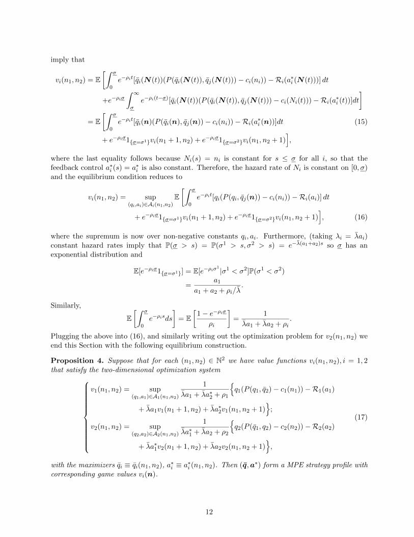
imply that

vi(n1, n2) = E[∫ σ

0e−ρit[qi(N(t))(P (qi(N(t)), qj(N(t)))− ci(ni))−Ri(a∗i (N(t)))] dt

+e−ρiσ∫ ∞σ

e−ρi(t−σ)[qi(N(t))(P (qi(N(t)), qj(N(t)))− ci(Ni(t)))−Ri(a∗i (t))]dt]

= E[∫ σ

0e−ρit[qi(n)(P (qi(n), qj(n))− ci(ni))−Ri(a∗i (n))]dt (15)

+ e−ρiσ1σ=σ1vi(n1 + 1, n2) + e−ρiσ1σ=σ2vi(n1, n2 + 1)],

where the last equality follows because Ni(s) = ni is constant for s ≤ σ for all i, so that thefeedback control a∗i (s) = a∗i is also constant. Therefore, the hazard rate of Ni is constant on [0, σ)and the equilibrium condition reduces to

vi(n1, n2) = sup(qi,ai)∈Ai(n1,n2)

E[∫ σ

0e−ρit[qi(P (qi, qj(n))− ci(ni))−Ri(ai)] dt

+ e−ρiσ1σ=σ1vi(n1 + 1, n2) + e−ρiσ1σ=σ2vi(n1, n2 + 1)], (16)

where the supremum is now over non-negative constants qi, ai. Furthermore, (taking λi = λai)constant hazard rates imply that P(σ > s) = P(σ1 > s, σ2 > s) = e−λ(a1+a2)s so σ has anexponential distribution and

E[e−ρiσ1σ=σ1] = E[e−ρiσ1 |σ1 < σ2]P(σ1 < σ2)

=a1

a1 + a2 + ρi/λ.

Similarly,

E[∫ σ

0e−ρisds

]= E

[1− e−ρiσ

ρi

]=

1

λa1 + λa2 + ρi.

Plugging the above into (16), and similarly writing out the optimization problem for v2(n1, n2) weend this Section with the following equilibrium construction.

Proposition 4. Suppose that for each (n1, n2) ∈ N2 we have value functions vi(n1, n2), i = 1, 2that satisfy the two-dimensional optimization system

v1(n1, n2) = sup(q1,a1)∈A1(n1,n2)

1

λa1 + λa∗2 + ρ1

q1(P (q1, q2)− c1(n1))−R1(a1)

+ λa1v1(n1 + 1, n2) + λa∗2v1(n1, n2 + 1)

;

v2(n1, n2) = sup(q2,a2)∈A2(n1,n2)

1

λa∗1 + λa2 + ρ2

q2(P (q1, q2)− c2(n2))−R2(a2)

+ λa∗1v2(n1 + 1, n2) + λa2v2(n1, n2 + 1),

(17)

with the maximizers qi ≡ qi(n1, n2), a∗i ≡ a∗i (n1, n2). Then (q,a∗) form a MPE strategy profile withcorresponding game values vi(n).

12

Remark 3. One can straightforwardly generalize the model in terms of the underlying point pro-cesses Ni. In particular, we may remove the assumption that Ni is increasing and/or has jumpsof size 1 only. Economically, this corresponds to the possibility that multiple technology stagescan be traversed at once, or that technology gains can be lost over time (in the sense of increasingproduction costs). The latter situation would be realistic for energy production where cheap con-ventional sources may become exhausted over time (think coal) leading to upward shocks in Ci(t).Assuming that the jump distribution of Ni is independent of (qi, ai) and identical across i = 1, 2,this generalization consists of replacing (17) with

v1(n1, n2) = supa1,q1

1

λa1 + λa∗2 + ρ1

q1(P (q1, q2, )− c1(n1)) −R1(a1)]

+ λa1

∑k

pkv1(n1 + k, n2) + λa∗2∑k

pkv1(n1, n2 + k), (18)

where pk := P(∆Ni = k|∆Ni 6= 0), k ∈ Z is the (integer) jump distribution for technology stagechanges.

3.1 Equilibrium Production

We proceed to solve the system (17) in the case where the controls are not coupled, Ai(n) = R2+∀n.

This decouples the optimization problems for qi, ai in (17). We also observe that the first term ineach supremum captures the instantaneous Cournot competition and contains only qi, while theother two terms represent the market shifts due to potential innovations and are related to ai.

Given current cost profile c(n), equilibrium production is determined as in the static case.Indeed, production rates only affect the immediate profits πi(c(n)) and hence can be optimizedpointwise in time (recall that we restrict to Markov feedback strategies). Thus, q∗i (n) can bedetermined from Lemma 1 for the static Cournot oligopoly after re-labeling the players in increasingorder of their costs.

In the examples below we focus on the linear price function which has zero relative prudence,ρ = 0. In that case, the following Corollary follows immediately from Proposition 3 and Lemma 1.

Corollary 1. Suppose P (Q) = η − Q (i.e. ρ = 0 in Corollary 3). Then recalling the notationB` =

∑`k=1 ck, we have

q∗i (c) = max(P − ci, 0) and π∗i (c) = q∗i (c)2, where P (c) = min

B` + η

`+ 1: 1 ≤ ` ≤ L

.

Moreover, with `∗ = max` : η +B`−1 − `c` > 0, we have

∂q∗i∂ci

= − `∗

`∗ + 1and

∂q∗i∂cj

=1

`∗ + 1.

Explicitly, the duopoly production rates are given by the solution of the static game with costsc(n):

qi(n) = q∗i (c(n)) =

η + cj(nj)− 2ci(ni)

3ifη + cj(nj)

2≥ ci(ni) ≥ 2cj(nj)− η;

η − ci(ni)2

if η + ci(ni) < 2cj(nj);

0 if η + cj(nj) < 2ci(ni).

(19)

The first case is the duopoly equilibrium, in the second case player i has a monopoly and in the lastcase player j has a monopoly. Under monopoly, one player has the market all to herself, choosingthe monopoly optimal level q∗i = (η − ci)/2. Figure 1 illustrates the resulting duopoly “wedge” asa function of costs c = (c1, c2), (and when η = 1).

13

Blockaded

0.5

1

0.5

Player 1Blockaded

Blockaded

0

Player 2

1 c1

c2

Figure 1: Type of Game Equilibrium in a Cournot Duopoly with linear demand P (Q) = 1−Q.

3.2 Equilibrium R&D Effort

In contrast, the R&D effort level ai enters (17) in a highly nonlinear fashion. Indeed, ai appearsboth in the numerator and denominator of the equations. Fixing a∗j , the first-order optimalityconditions for ai are obtained by differentiating (17) with respect to ai. To find the equilibriumlevel (a∗1, a

∗2) then requires solving the resulting system of two nonlinear equations.

More precisely, recalling the notation π∗i (c(n)) for the revenue from production as in (8), andfixing a∗j , set

Ji(a, a∗j ;n) := E

[1− e−ρiσ

ρi(π∗i (c(n))−Ri(a))+e−ρiσ1σ=σ1vi(n1+1, n2)+1σ=σ2vi(n1, n2+1)

].

(20)

Then a∗i (n) = arg supa≥0 Ji(a, a∗j ;n). As with production rates, R&D efforts cannot be negative.

If the marginal cost of R&D R′i(a) is bounded away from zero, it is possible that the equilibriumR&D effort is zero. Indeed, fixing i = 1 for concreteness,

∂

∂a1J1(a1)

∣∣∣a1=0

=1

λa∗2 + ρ1

[−R′1(0) + λv1(n1 + 1, n2)− π∗1(c(n)) + λa∗2v1(n1, n2 + 1)

a∗2 + ρ1/λ

].

Since depending on model parameters v1(n) and π∗1(c(n)) can be arbitrarily close to zero, it isclear that if R′1(0) > 0 then the above expression may be negative and hence a∗1(n) = 0. In thatcase, player 1 would invest nothing in R&D and only player 2 innovates, leading to P(σ = σ2) = 1.Similarly, it is also possible that a∗1 = a∗2 = 0 in which case technologies of both players remainforever frozen. With constant production costs, the corresponding Nash equilibrium for q reducesto a stationary Cournot game with cost profile c(n), which is equivalent to the one-shot staticmarket.

Existence of an equilibrium pair (a∗1, a∗2) is resolved through the usual method of analyzing the

invertibility of the best-response functions, see Grossman and Shapiro [1987], Judd [2003].

3.3 Solving for the Equilibrium Strategies

Once the current equilibrium strategies a∗i (n1, n2), qi(n1, n2) are determined, the overall system(17) can be viewed as a double array of nonlinear optimization problems, coupled within each

14

other and indexed by n. The standard paradigm of dynamic programming could then be invokedto solve iteratively “backwards” in n for the vi’s. Indeed, given vi(n1 + 1, n2), vi(n1, n2 + 1) onecan determine vi(n1, n2) so that starting with some terminal conditions vi(N1, ·), vi(·, N2) one mayiteratively solve for the full double array of game values. This gives a well-defined numerical recipefor any finite technology ladder Ci. The next Lemma shows that the finiteness assumption is nottoo restrictive.

Lemma 2. Suppose that λi = λai and R′i(0) > 0. Then the dynamic game can be reduced to afinite-stage one, i.e. for ni’s large enough for all i, ai(n) = 0. Conversely, if R′i(0) = 0 and theladder Ci is strictly decreasing then a∗i (n) > 0 for all n.

The proof is given in Appendix B. Because the technology ladders are monotone and Ci(t) ≥ 0,the production costs live in a bounded interval. Hence, if the number of stages is unbounded, theremust be at least one accumulation point ci for the ladder Ci. Consequently, after sufficiently manyinnovations, ci(n) will be very close to ci and the potential for gain becomes arbitrarily small. If themarginal cost of R&D is strictly positive then R&D efforts will strictly dominate any innovationprofits and R&D is shutdown. Conversely, if R′i(0) = 0, then for small enough level of R&D effort,the R&D gains (which are asymptotically linear in ai) dominate the negligible R&D expenditures.

Lemma 2 highlights the crucial role of R′i(0). If R′i(0) = 0 then ai(n) > 0 for all n, since themarginal cost of effort is negligible for a sufficiently small. Consequently R&D is always employedand the game never ends (unless the technology ladder is finite). On the other hand, if R′(0) > 0,then eventually the marginal cost of R&D strictly dominates any resulting gains and further R&Dbecomes economically non-feasible. Thus, there must be absorbing game stages, where the playersendogenously forgo R&D. We believe the latter situation is both more realistic economically, andalso computationally easier, permitting to employ backward recursion to find game values. Gameswith infinite stages create technical difficulties in defining an equilibrium strategy. Motivated bythis discussion, we henceforth focus on the case

R(a) =1

2a2 + κa, (21)

which combines features of the classical quadratic cost structure and the strictly positive marginalcost controlled by the parameter κ = R′(0).

The proof of Lemma 2 implies the following:

Corollary 2. In the linear duopoly model with the lower bound on costs ci = 0, a sufficient conditionto guarantee a1(n) = 0 is

|π∗1(0, c2(n2))− π∗1(c1(n1), 0)| ≤ ρ2R′1(0).

In particular if max(c1(n1), c2(n2)) ≤ min(ρ21R′1(0), ρ2

2R′2(0)) then a(n) = 0 and the resulting gamestage features no R&D.

If a(n) ≡ 0 then the resulting market is equivalent to a static Cournot game with cost profile

c(n). In particular, we immediately obtain vi(n) =π∗i (c(n))

ρi. Taking n big enough to satisfy the

conditions of Lemma 2 allows to use the above as boundary condition for the backward recursionon the lattice n ⊂ N2 for (17). Note that when solving for a(n) it is possible that a(n) = 0 emergesas the solution even in an “interior” game stage, which however poses no numerical concerns.

15

3.4 Game Evolution

For the remainder of the paper we work with a fixed MPE profile (q,a) and drop the corresponding∗’ and over-bar. The discrete nature of the state N implies that the global game is partitioned intostages, with innovation epochs characterizing transitions among different stages. The piecewise-constant behavior of N moreover makes each stage equivalent to a stationary Cournot game withstate-dependent payoffs. Namely, at each stage players compete in a static Cournot market whilealso engaging in R&D that will eventually move them to a new stage. Until R&D comes to fruition,players solve the local problem; as soon as there is an innovation by a “winning” player at time σ,a new optimization problem is considered in turn. The fact that the controls in the constructedMPE are a function of N(t) imply the following

Proposition 5. The technology state variable N is a state-dependent Markov chain on N2. Giventhe current stage (n1, n2), the sojourn time in this state has a memoryless Exponential distributionwith mean 1

a1(n)+a2(n) and the next transition is to (n1 + 1, n2) (resp. (n1, n2 + 1)) with probabilitya1(n)

a1(n)+a2(n) (resp. a2(n)a1(n)+a2(n) ).

Thus, the global evolution is characterized by patching together the local equilibria describedby q,a. One can generate time-scenarios of the dynamic Cournot market as follows. Given n, wedraw two independent Exponential r.v.’s σi ∼ Exp(λai(n1, n2)), i = 1, 2 and take σ = σ1 ∧ σ2. Wealso solve for q(n) using (19). This yields the game solution on [0, σ) and based on the relationshipbetween σ1 and σ2 the next game stage N(σ) = (n1 +1σ1<σ2, n2 +1σ2<σ1). After transitioning,the new production rates q(N(σ)) are updated and the above process is repeated with fresh drawsfor σi. By Lemma 2, this chain will reach an absorbing state (where a = 0) with probability 1, sothat all other states are transient and the above algorithm is guaranteed to terminate.

Remark 4. The local structure of the Cournot games that arise allows further indexing of gameparameters by n. For example, for a realistic calibration it would be reasonable to assume thatthe R&D costs depend on the current technology, i.e. R(a) = R(a;n). Similarly, one can alsoindex the discount factors or the demand curves by n and retain the Markov structure for dynamicprogramming.

Remark 5. We have focused in this section on the duopoly competition (L = 2) to illustrate theeffects of competition in a presentable way. Two extreme cases are also of interest: the monopolycase L = 1 and the limit L =∞. In the next section, we analyze the case where only one player caninnovate, but interacts with a second player through Cournot competition. This is contrasted withthe case of two innovators in Section 5, specifically the discussion at the end of that section. Thisgives some insight into the effect of the number of players that are involved in R&D. In adding moreplayers, choices have to be made as to what their costs of production are if comparisons are to bemade, and perhaps only the symmetric situation of adding more identical players makes sense forcomparison, where here we are very much interested in heterogeneous situations, even if the playersdiffer only in their initial costs. Analyzing a dynamic game where players may enter over timeas their costs drop is interesting too, but requires a separate work. For instance, a case withoutinnovation where players enter as others use up an exhaustible resource is studied in Ledvina andSircar [2012].

The limit L→∞ of a large number of players relates to much current research in (continuum)mean field games. These can be tractable in some situations, but again require a separate andmathematically involved analysis which is beyond the scope here. We refer to Chan and Sircar[2014], Chan and Sircar [2015] and Gueant et al. [2011] for recent developments in mean fieldgames and Cournot competition.

16

4 Unilateral R&D

We begin our illustrations with a toy model wherein only a single player (for concreteness P1) canengage in R&D. This can be viewed as a special case where the second player is constrained toa2 ≡ 0. Since C2(t) ≡ c2 is now fixed, the stochastic state is the one-dimensional (N1(t)) and thesystem (17) reduces to a coupled array of optimization problems for vectors rather than matrices.Unilateral R&D can be visualized as a horizontal movement in the diagram of Figure 1, from rightto left at the given level c2. Note that interpreting equilibrium earnings of player 1 as a generictechnology-dependent reward function, the model with a single innovator is abstractly equivalentto incorporating intermediate rewards into the multi-stage racing game studied by Judd [2003].

For the remainder of this section we fix c2 and drop it from arguments of all relevant functions.Also for concreteness we take the linear inverse demand curve P (Q) = η − Q from Corollary 1,yielding

π∗i (c(n)) = (q∗i ((c1(n), c2)))2 .

By Lemma 2, without loss of generality the technology of P1 has a finite number of stages n. Atthe ultimate stage, no more R&D research is possible for either player and we face the static-costCournot market with game values

v1(n) =π∗1(c1(n), c2)

ρ1, v2(n) =

π∗2(c1(n), c2)

ρ2.

The rest of the game values are determined via the system of difference equations (obtained bysetting a2 ≡ 0 in (17))

v1(n) = supa≥0

1

λa+ ρ1

π∗1(c1(n), c2) + λav1(n+ 1)−R1(a)

. (22)

The above is a nonlinear equation for a1(n) with v1(n+ 1) entering as a coefficient. For instance,assuming quadratic costs of (21), a1(n) is the root of the quadratic from the first-order-conditionequation

−ρ1λv1(n+ 1) + (a+ κ)(λa+ ρ1) + λ(π∗1(c1(n), c2)− (a2/2 + κa)) = 0.

The game values for player 2 are similarly determined from

v2(n) =1

λa1(n) + ρ2

π∗2(c1(n), c2)2 + λa1(n)v2(n+ 1)

.

Globally, (22) can give rise to three market structures based on the cases in (19): P1 monopoly,P2 monopoly, and duopoly. In particular, for η/2 < c2 < η, as player 1 innovates all three structuresarise dynamically. Indeed, as C1 is reduced, the market moves from old-generation monopoly byplayer 2, to duopoly, and finally to new-generation monopoly of player 1. The phase transitionstake place at C1 = η+c2

2 and C1 = 2c2−η, respectively, cf. Figure 1. (If c2 < η/2, P1 never achievesmonopoly.)

Figure 2 illustrates this solution in the case of a linear technology ladder c1(n) = 1 − µn andP (Q) = 1−Q. We show three investment curves n 7→ a1(n) for different costs of the other playerc2. In scenario (a), c2 = 0.7 which represents weak competition; in particular once c1(n) ≤ 0.4, P2is blockaded and P1 has monopoly. In scenario (b), c2 = 0.4 is proxy for moderate competition;scenario (c) c2 = 0 illustrates strong competition since c2 ≤ c1(n) for all n. In both of the lattercases P2 always produces and is never blockaded. In all three cases we also have that for c1(n)large (n small), P1 is blockaded, q∗1(c1(n), c2) = 0. These stages are illustrated with filled symbolsin Figure 2 (for example in case (a), q∗1(c1(n), c2) = 0 for n ≤ 7).

17

0 10 20 30 40 50

0.00.1

0.20.3

0.4

Technology Stage n

R&D

Effor

t a1(n

)

1.00 0.80 0.60 0.40 0.20 0.00

P1 Costs c1(n)

(a): c2=0.7(b): c2=0.4(c): c2=0

Figure 2: Effort curves for unilateral R&D in a Cournot duopoly. The technology ladder is c1(n) =1− 0.02n, n = 0, . . . , 50 with effort costs R(a) = a2/2 + 0.3a, ρ1 = 0.01 and P (Q) = 1−Q. Filledsymbols indicate stages where q∗1(c1(n), c2) = 0.

4.1 Value of R&D

With unilateral R&D the Markov chain N is a birth process (Markov counting process), andthe game evolution simply proceeds sequentially through stages (c1(1), c2), (c1(2), c2), . . . . Denoteby 0 = τ0, τ1, τ2, . . . the respective transition times to the next technology stage. The τk’s aredetermined by the effort levels a1(n), namely τn − τn−1 ∼ Exp(λa1(n)), so that E[τn − τn−1] =(λan)−1. We can express the value of player 1 via

v1(1) = E0

[∫ τ1

0e−ρ1s(π∗1(c1(1), c2)−R(a1(1))) ds+

∫ τ2

τ1

e−ρ1s(π∗1(c1(2), c2)−R(a1(2))) ds

+

∫ τ3

τ2

e−ρ1s(π∗1(c1(3), c2)−R(a1(3))) ds+ . . .+

∫ ∞τ n

e−ρ1sπ∗1(c1(n), c2)ds]

=

n−1∑n=1

(π∗1(c1(n), c2)−R(a1(n)))

ρ1E0

[e−ρ1τn−1 − e−ρ1τn

]+π∗1(c1(n), c2)

ρ1E0[e−ρ1τ n ]

=

n+1∑n=1

π∗1(c1(n), c2)−R(a1(n)) ·

1

λa1(n) + ρ1

n−1∏j=1

(λa1(j)

λa1(j) + ρ1

) , (23)

where the last equality is based on the expansion e−ρ1τn = e−ρ1τ1e−ρ1(τ2−τ1) · · · e−ρ1(τn−τn−1) and

the moment generating function of Exponential random variables. The above formula links thestagewise payoff rates π∗1(c1(n), c2) and R&D rates a1(n) to the game value of player 1.

This view also highlights the value of R&D. Compared to the base scenario of zero R&Dinvestment, the gap

G1(n) = v1(n)−∫ ∞

0e−ρ1sπ∗1(c1(n), c2) ds = v1(n)− π∗1(c1(n), c2)

ρ1(24)

precisely captures the NPV of R&D investments. Note that G1(n) = 0 is equivalent to a1(n) = 0and represents the end of the technology ladder. We find, cf. right panel of Figure 3, that the

18

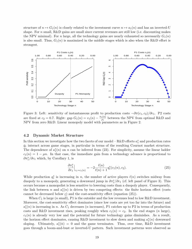
structure of n 7→ G1(n) is closely related to the investment curve n 7→ a1(n) and has an inverted-Ushape. For n small, R&D gains are small since current revenues are still low (i.e. discounting makesthe NPV minimal). For n large, all the technology gains are nearly exhausted so necessarily G1(n)is also small. Thus, G1(n) is maximized in the middle stages which is also when the R&D effort isstrongest.

0 10 20 30 40 50

0.0

0.1

0.2

0.3

0.4

0.5

0.6

Technology Stage n

Prof

it se

nsitiv

ity

Duopoly P1 Monopoly

1.00 0.80 0.60 0.40 0.20 0.00

P1 Costs c1(n)

0 10 20 30 40 50

01

23

45

6

Technology Stage nR&

D G

ap G

1(n)

1.00 0.80 0.60 0.40 0.20 0.00

P1 Costs c1(n)

Figure 3: Left: sensitivity of instantaneous profit to production costs −∂π(c1, c2)/∂c1. P2 costs

are fixed at c2 = 0.7. Right: gap G1(n) = v1(n)− π1(n)ρ1

between the NPV from optimal R&D andNPV from zero R&D. Linear monopoly model with parameters as in Figure 2.

4.2 Dynamic Market Structure

In this section we investigate how the two facets of our model – R&D efforts a∗1 and production ratesq1 interact across game stages, in particular in terms of the resulting Cournot market structure.The dependence of a∗1(n) on n can be inferred from (23). For simplicity, assume the linear ladderc1(n) = 1 − µn. In that case, the immediate gain from a technology advance is proportional to∂π∗1/∂c1 which, by Corollary 1, is

∂π∗1∂c1

∣∣∣c1=c1(n)

= −2`(n)

`(n) + 1q∗1(c1(n), c2). (25)

While production q∗1 is increasing in n, the number of active players `(n) switches midway fromduopoly to a monopoly, generating a downward jump in ∂π∗1/∂c1 (cf. left panel of Figure 3). Thisoccurs because a monopolist is less sensitive to lowering costs than a duopoly player. Consequently,the link between n and a∗1(n) is driven by two competing effects: the finite horizon effect (costscannot be decreased below c) and the cost-sensitivity effect (equation (25)).

When C1 is large (n small), P1 is the outsider and the low revenues lead to low R&D investment.Moreover, the cost-sensitivity effect dominates (since low costs are yet too far into the future) anda∗1(n) is increasing in n. As C1 decreases (n increases), P1 catches up to P2 in terms of productioncosts and R&D investment rises, peaking roughly when c1(n) = c2. In the end stages (n large),c1(n) is already very low and the potential for future technology gains diminishes. As a result,the horizon effect dominates, causing R&D investment to slow down and making a∗1(n) downwardsloping. Ultimately, a∗1(n) = 0 and the game terminates. Thus, over time, R&D investmentgoes through a boom-and-bust or inverted-U pattern. Such investment patterns were observed as

19

early as Kamien and Schwartz [1978], though in their work it was due to the exhaustibility of theunderlying production resource, whose depletion eventually makes R&D worthless.

Next, we discuss the impact of R&D on the production rates. As indicated by Lemma 1, lowerproduction costs C1 increase q1 and Q. R&D naturally crowds out player 2 whose productionq2 declines, creating a substitution effect whereby increased production from player 1 is partiallyoffset by decreased output of player 2. It follows that the price Pt = η − q1(N(t)) − q2(N(t)) isnon-increasing over time. Moreover, this price decline accelerates once player 1 achieves monopoly,since in monopoly the above substitution effect goes away.

The inverted U-shape of the investment curve is broadly similar across all three scenarios inFigure 2, though several variations appear. Notably, scenario (a) features a double boom-and-bustpattern. This occurs due to a structural shift in the market as P1 achieves monopoly for n ≥ 0.The different sensitivity to production costs (monopolist having smaller cost-convexity ∂2π∗1/∂c

21)

between a monopolist and a duopolist causes the R&D investment to slightly increase again aroundn = 30 after falling for several stages. We also note that c2 7→ a∗1(n; c2) is not monotone— e.g., theinvestment curves for c2 = 0.7 and c2 = 0.4 cross. This illustrates the non-monotone relationshipbetween market competitiveness and R&D investment – while very strong competitors (scenario(c)) discourage R&D by diminishing future gains, moderate competition can actually spur R&Das producers try to get an edge. Moreover, the peak of R&D efforts depends strongly on c2 – inscenario (b) R&D is maximized around stage n = 35, while in scenario (a) it is peaking much earlieraround n = 25.

Figure 2 also demonstrates the nontrivial interaction between market structure and R&D. Recallthat either q1(n) = 0 (blockading) or a∗1(n) = 0 (technological stagnation) are possible, leading tofour regimes for the production + R&D controls. All four cases may be observed in Figure 2. First,the case q1(n) = 0 takes place when c1(n) is too big and P1 is blockaded. In that case, P1 receives nocurrent revenues and hence any respective R&D investment is solely about hoping for future profits.Those may or may not be enough to justify current effort. To wit, in scenario (a) for n ∈ 5, 6, 7we have a∗1(n) > 0 even with q1(n) = 0. This is the proverbial “invest now for the better future”situation. Simultaneously in the same scenario when n ≤ 4, a∗1(n) = 0 = q1(n) – the “light in theend of the tunnel” is too far away so that R&D is not undertaken. Indeed, with n = 4 one needsat least 4 technology improvements to generate any revenue; the associated revenues are so far intothe future that they are not sufficient to finance the immediate R&D expenditures, cf. (23). Asa result, P1 invests nothing in R&D and will remain forever blockaded, leading to v1(n) = 0 forn ≤ 4. In contrast for n ≥ 5, only 3 or fewer technology improvements are necessary to break P2’smonopoly and enter the market and R&D becomes economically worthwhile. A similar situationhappens in scenario (b). However, in scenario (c) we see the opposite effect— at stage n = 27 andc1(n) = 0.48, q1(n) > 0 but a∗1(n) = 0. In other words, even with positive present cashflows, theexpected gain from technology investment is not big enough to justify it. This happens becauseP2 is too strong so P1 will continue to have a small market share for the foreseeable future. As aresult, P1 “gives up” on R&D despite being in the market.

4.3 Policy Implications

The above observations could be translated into policy recommendations. We imagine that P2represents an entrenched incumbent (for example fossil fuel energy generators) and P1 is a new-technology entrant that policy makers wish to support (eg. a new method for green energy pro-duction). In an ideal world, the future benefits of P1’s tools would allow to privately finance therequisite R&D even before the new method is generating any revenues. However, if these gains aretoo remote, policy intervention via R&D subsidies might be necessary to get a head start. For ex-ample, starting at n = 0 and scenario (a), subsidized R&D is needed for the first 4 stages otherwise

20

R&D Effort

Costs P1

Cos

ts P

2

0.78 0.37 0.17 0.08

0.78

0.37

0.17

0.08

Production

Costs P1

0.78 0.37 0.17 0.08

0.0

0.1

0.2

0.3

0.4

0.5

0.6

Figure 4: Duopoly R&D race with linear price function P (Q) = 1−Q. Right panel shows the efforta∗1(n1, n2) and left panel the production rate q1(n1, n2). Quadratic costs Ri(a) = a2/2 + 0.1a withλi(t) = 5ai(t), ρ = 0.1. ci(n) = e−n/8, n ∈ 1, . . . , 252.

the new technology will never be developed on its own. However, once n ≥ 5, the subsidy can bewithdrawn and replaced with private financing. One could imagine various tax/equity mechanismsthat recoup these seed investments in the ultimate future n = 50. Scenario (c) shows that suchkick-start subsidies could be needed even if P1 is already in the market but the initial R&D hurdleis too high (the situation where a∗1(n) = 0, q1 > 0). Overall, Figure 2 supports the idea of seedsubsidies that can then be withdrawn once the new technology is sufficiently competitive. Subsidiesare especially attractive if one imagines the government to have lower discount rates compared tothe game players, facilitating long-maturity loans.

5 Bilateral R&D Race

To illustrate a truly dynamic R&D race, we next investigate a duopoly L = 2 with bilateralR&D strategies a1(t), a2(t). We continue to maintain linear inverse demand P (Q) = η − Q. Forexpositional clarity we focus on the symmetric case where the R&D costs R(a), discount factorsρi ≡ ρ, and technological ladders Ci of both players are identical. Of course, during the evolutionof the game, the players will end up in different stages, making the sub-games non-symmetric. Interms of the diagram in Figure 1, the games moves from upper-right to lower-left by taking stepseither to the South or West.

Figure 4 shows the optimal feedback controls for a geometric technology ladder ci(n) = exp(−µn)and quadratic costs (21). Since absolute progress slows down, there is an economically optimallimit level n such that no R&D takes place beyond stage (n, n). Based on Lemma 2, we can taken = −µ−1 log(ρ2κ). After reducing to a finite-stage setting, we can inductively solve for vi(n) overthe resulting square lattice ni ∈ 1, . . . , n, i = 1, 2.

The two panels of Figure 4 show the feedback controls q1(n), a∗1(n) of player 1 as a function ofn. By symmetry, the solution for P2 is simply the mirror image q2(n1, n2) = q1(n2, n1), etc. Inthe right panel we plot the equilibrium production rate q1(n1, n2) which as expected is maximized

21

when n1 is large and n2 is small, i.e. C1 C2. In the first few stages (n1 < 5), it is possible that P1is blockaded (q1(n1, ·) = 0 in the upper-left corner). In the left panel, we show the correspondingeffort level a∗1(n1, n2). For n1 = 25 = n (right boundary), a∗1(n, ·) ≡ 0 no more R&D is undertaken.Similarly, no R&D is undertaken when n1 n2 (upper-left corner) in which situation P1 is too“behind” P2 and is moreover blockaded, making eventual R&D gains too minuscule to be feasible.However, we note that the region (n1, n2) : a∗1(n1, n2) = 0 is much smaller than the blockadingregion for P1, so that in many game scenarios P1 may be blockaded but innovating, hoping to catchup to P2 eventually.

Most interestingly, Figure 4 demonstrates that the R&D investment is maximized when n1 isslightly larger than n2. This is the situation where P1 has a small technological advantage over P2,whereby she has the highest motivation (and the funds) to increase the gap with her competitor.In that sense, a symmetric competition N1(t) = N2(t) is unstable, since whichever player is ahead,is also putting more in R&D than the player that is behind. This feature confirms Lemma 1 whichshows that ceteris paribus a more dominant player is more sensitive to her costs and hence moreincentivized to innovate.

Over time, the R&D race reaches one of the absorbing stages where a∗i (n1, n2) = 0∀i. In thepresent example this effectively reduces to limt→∞N(t) = (n, n) (there is also a small absorbingregion in the extreme case of n1 n2 which is however extremely unlikely starting from N1(0) =N2(0)). Figure 5 shows the distribution of (N1(t), N2(t)) over t = 2, 8, 15, 25 based on the initialcondition N(0) = (1, 1). We observe that the duopoly instability causes a rather large spread(or “variance”) at intermediate times t = 8, 15 where a significant number of sub-stages could berealized. As t→∞, the game collapses back to the main attractor in the upper-right corner.

5 10 15 20 25

510

1520

25

P1 Technology Stage

P2

Tech

nolo

gy S

tage

5 10 15 20 25

510

1520

25

P1 Technology Stage

P2

Tech

nolo

gy S

tage

5 10 15 20 25

510

1520

25

P1 Technology Stage

P2

Tech

nolo

gy S

tage

5 10 15 20 25

510

1520

25

P1 Technology Stage

P2

Tech

nolo

gy S

tage

t = 2 t = 8 t = 15 t = 25

Figure 5: Distribution of (N1(t), N2(t)) in N2 in a duopoly R&D race. All parameters are as inFigure 4. Each panel shows a 2-D histogram of (N1

t , N2t ) based on 500 simulated paths; size of each

gridpoint is proportional to the empirical frequency. The initial condition was N(0) = (1, 1).

Comparing back to the setting of Section 4, the difference between the unilateral and bilateralsettings sheds light on the impact of R&D competition on the competitive behavior of the producers.From the point of view of P1, if she has the sole access to innovation and engages in unilateralR&D then she is able to fully reap the resulting benefits; in contrast bilateral R&D competitionnecessarily dilutes gains from lower costs as P2 is expected to catch up over time and maintaincompetitive pressures. This intuition suggests that the P1 game value ought to be larger underunilateral R&D than under bilateral R&D, and consequently that her effort should be lower (sincethe NPV of R&D is generally less). While the former statement is true, the latter is not. To wit, inour numerical experiments we found that in some scenarios, fixing P2 production costs at a givenlevel c2 and comparing the resulting aUn1 (n) (from Section 4) against aBi1 (n) (from this Section), the

22

bilateral-R&D effort is higher. In other words, removing R&D competition makes immediate R&Dresearch less urgent for P1, leading to lower optimal effort. This finding could be connected to theconcept of pre-emption, whereby bilateral R&D forces producers to exert additional effort in orderto stay ahead (or not fall behind) competitors, which in turn further erodes their profitability.

6 Effect of Uncertainty

In the model (4) the only stochastic source are the counting processes Ni controlling technologicaladvances. It is of interest to understand the impact of the discrete shocks in Ni on the gamestructure. In particular, a natural question is whether uncertainty impedes or encourages R&D.To shed some insight, we consider refinements of the technology ladder C. Namely, starting with aladder C, consider a refined ladder C′ which satisfies

c′(2n) = c(n) and c′(2n+ 1) =c(n) + c(n+ 1)

2.

To compensate for having more stages, we also double the scaling constant λ′ = 2λ. Informally,the refined model represents the situation where R&D discoveries are half the size but occur twiceas frequently (for same amount of effort). Let (N ′(t)) be the counting process in the refined model.With this setup and keeping ai(t) fixed, we observe that

E[Ni(t)] = E[N ′i(t)/2

], Var(Ni(t)) = 2Var

(N ′i(t)/2

).

Therefore, using N ′/2 as the measure of technology progress in the refined model, the refined modelhas same rate of R&D discoveries, but only half of the corresponding variance.

As the degree of refinement is increased, the variance of R&D innovations converges to zero.Thus, the above construction offers a way to interpolate between the deterministic model (zerovariance) and the stochastic version analyzed so far. To be precise, consider a continuous decreasingmap f(x) ∈ [0, 1], x ∈ [0, x], where x represents the continuous level of “progress”. Innovation maygo on indefinitely, or have some finite bound x. The map x 7→ f(x) defines the technology ladder,e.g. f(x) = exp(−µx). Now for any M ∈ Z, let c(n;M) = f(n/M), n = 1, . . . , which gives riseto a ladder C(M) with a corresponding scaling Mλ. We refer to M as the refinement level. Thecase of finite M nests the discrete technology ladders while in the limit M → ∞, one obtains adeterministic model where progress is completely dependent on the R&D level without any intrinsicuncertainty. For ease of comparison across different refinement levels, for the remainder of thisSection we re-parameterize both q and a in terms of x, q(x;M) = q(c(n;M)) keeping in mind thatx ∈ n/M : n = 1, . . . , .

The impact of uncertainty on the game equilibrium can now be analyzed by the dependence ofthe equilibrium strategies on M . Note that q(x) = q(f(x)) only depends on the present costs andhence is independent of M ; in contrast a(x) is driven by the amount of uncertainty corresponding tothe refinement level. AsM rises, the corresponding dynamic game has more and more stages, so thatplayers have more opportunities to adjust their feedback-form controls and therefore extract morevalue. However, uncertainty also benefits the players because it allows for potentially rapid progresswhich is assigned extra weight due to the discounting involved. Indeed, the map τ 7→ exp(−ρτ)is convex, so that a mean-preserving transformation of τ will affect the corresponding expectation(cf. (23)) inversely in terms of its variance. The next Lemma shows that the overall impact of Mon game values is as a result ambiguous.

Lemma 3. Consider a technology ladder C(M) and a doubled ladder C(2M). Then v(2M)(x) may beeither bigger or smaller than v(M)(x).

23

1.0 0.8 0.6 0.4 0.2 0.0

0.0

0.5

1.0

1.5

P1 Costs c1(n)

v 1(n

, n2)

c1(n) = 1−n/10, λ=4c1(n) = 1−n/20, λ=8c1(n) = 1−n/50, λ=20

1.0 0.8 0.6 0.4 0.2 0.0

0.0

0.2

0.4

0.6

P1 Costs c1(n)

a 1(n

, n2)

Figure 6: Comparison of game values v1(·, n2) and effort levels a∗1(·, n2). Bilateral symmetric R&Dgame with ρ = 0.1 and R(a) = a2 +0.2a and linear technology progress c1(n) = 1−n/M , λ = 0.4Mfor M = 10, 20, 50. We show the results for P1 at the fixed level c2 = 0.7 of P2 costs.

Put another way, less uncertainty lowers the probability of extra profits from rapid progressbut allows more flexibility in R&D investments over time. The above results should be contrastedwith the findings of Lafforgue [2008] in the single-agent setting. Lafforgue finds that uncertaintyunambiguously lowers innovation (and therefore overall utility). This is because the stationarysolution obtained in Lafforgue [2008] eliminates any extra potential gains from favorable innovationscenarios. In contrast, in our model the additional gains that arise from for example the duopoly-to-monopoly transition, percolate through the game stages and make the unlikely but potentiallyvery lucrative rapid innovation paths strategically important. Thus, increased uncertainty cansometimes benefit the player and make her even more enthusiastic about R&D. (The non-monotoneR&D effort in Figure 2 is again instructive here.)

Figure 6 shows the impact of R&D success volatility in a symmetric bilateral model. We takethe linear ladder f(x) = 1 − µx, x ∈ [0, 1/µ]; in this case refinement is equivalent to takingc1(n;M) = 1 − n/M , n = 1, . . . ,M and varying M . To illustrate Lemma 3 we observe that asM changes, both R&D efforts ai(x) and game values vi(x) have ambiguous changes, sometimesincreasing and sometimes decreasing.

6.1 Deterministic Limit

The deterministic case is obtained by taking the formal limit M → ∞, which corresponds toC(M) → f . The fluid limit of Ni(t)/M yields that the underlying technology state x slides downthe ladder x 7→ f(x) at the speed proportional to ai(t), i.e. dxi(t) = ai(t) dt or equivalently forCi(t) = f(xi(t))

dCi(t) = f ′(f−1(Ci(t))) · ai(t) dt.

For presentational clarity, we revisit the deterministic version of the unilateral R&D model,where only P1 innovates and the technology ladder is linear f(x) = 1− λx, so that

dC1(t)/dt = −λa(t).

Fix c2 and denote by gi(c) the value function of player i starting with initial P1 costs C1(0) = c.To distinguish from the stochastic model, the corresponding controls are denoted a(c) and q(c).

24

Taking quadratic R&D costs (21), g1 solves the nonlinear ODE

ρ1g1(c) = π∗1(c, c2) +(−λg′1(c)− κ)2

+

2= 0, c ∈ [0, 1], (26)

where π∗1(c, c2) is the equilibrium profit under cost profile (c, c2) (see Lemma 1) and the initial

condition is g(0) =π∗1(0,c2)ρ1

. Note that g1 is decreasing, hence the minus sign in front of g′1. The

optimal controls are q(c) = q∗1(c, c2) from (19) and a(c) = (−λg′1(c)−κ)+. The relationship in (26)subsumes the static case a(c) = q(c) = 0 whereby g1(c) = 0, and also the case of zero R&D thatimplies g1(c) = ρ−1

1 π∗1(c, c2) or in differential form ρ1g′1(c) = ∂

∂cπ∗1(c, c2).

Note that at c = 0,(−λg′1(0)−κ)2

+

2 = ρ1g1(0) − π∗1(0, c2) = 0, so the boundary condition issingular (g′(0) is undetermined). For a numerical solution we instead use limc↓0 g

′1(c) = −κ/λ which

corresponds to the condition that R&D efforts are smoothly wound down to zero as the ultimatetechnology state is approached. As before, one can view ρ−1

1 π∗1(c, c2) ≤ g1(c) as an “obstacle” forg1, with ρ1g1(c) = π∗1(c, c2) if and only if a(c) = 0. The gap G(c) := g1(c)− ρ−1

1 π∗1(c, c2) representsthe NPV of R&D gains and substituting into (26) is shown to have a quadratic relationship to theR&D effort level a(c),

G(c) =1

2ρ1a(c)2. (27)

Relationship (27) sheds light on the link between the right panel of Figure 3 and the effort curvesin Figure 2.

Moreover, recall that the profit function π∗1(c, c2) itself is piecewisely defined in terms of thethree possible market structures (duopoly or monopoly of either producer). As a result, the fullsolution for g1(c) is defined piecewise over as many as four intervals, with both pre-specified andfree boundaries arising. The ODE (26) clarifies the phase transitions resulting from changes inmarket structure. Indeed, formally differentiating (26) we obtain

ρ1g′1(c) =

∂

∂cπ∗1(c, c2)− λg′′1(c) · (−λg′1(c)− κ)+.

We now observe that since c 7→ π∗1(c, c2) is continuous, by (26) so is c 7→ g′(c) (and hence c 7→ a(c)).At the same time, at levels where the market changes from a monopoly to a duopoly and vice-versa,the cost-sensitivity of profit changes. This implies that g′′(c) must be discontinuous, introducinghigher-order discontinuities into g1. In particular, because a monopolist is less sensitive to hercosts, at the transition level c = 2c2 − 1, we have

− ∂

∂cπ∗1(c, c2)

∣∣∣c=(2c2−1)−

< − ∂

∂cπ∗1(c, c2)

∣∣∣c=(2c2−1)+

,

and this jump may cause the sign of g′′(c) to change from negative to positive when transitioning toP1 monopoly. In other words, the g may go from concave to convex, and a may go from decreasingto increasing, generating a kink at c = 2c2 − 1.

Figure 7 illustrates these effects for the case c2 = 0.6. In that case, there are two fixed phaseboundaries at c = 0.8 and c = 0.2 which indicate blockading of P1 and P2 respectively. The Figureconfirms the mentioned double inverted-U relationship for c 7→ a(c). In particular, there is a kink atc ' 0.45 (where − ∂

∂cπ∗1(c, c2) = ρ1κ/λ) which causes R&D to be started with a “jolt”, and another

kink at c = 0.2 = 2c2 − 1 which causes R&D trend to suddenly change from negative to positive.Economically, the time-trend of current R&D investments is tied to the change in expectations of

25

future gains from lowered costs. Thus, as C1(t) drops below 0.3, the gains to P1 from R&D diminishas she anticipates lower cost-convexity (the downward jump in ∂

∂cπ∗1(c, c2) observed in Figure 3)

once in monopoly. As a result, R&D effort is lowered. However, once monopoly is actually achieved,t 7→ ∂π∗1(Ct, c2)/∂c resumes its growth and the R&D trend is reversed.

Figure 7 also compares the deterministic R&D effort curve a(c) to the discrete versions a(M)(c)obtained with a finite M . We observe that while for M = 10 the discretization makes a significantdifference, already with M = 100 stages, the stochastic setting is very close to the deterministicone. Notably, for c = 0.4 and M = 10, the large uncertainty (and hence potential for quick gains)makes it optimal to do some R&D, while for M = 100 and the deterministic case, at the sameproduction cost level c the expected gains are not sufficient to justify investments. This highlightsthe extra benefits that uncertainty may offer and shows that correct modeling of uncertainty is animportant aspect of the framework.

1.0 0.8 0.6 0.4 0.2 0.0

0.00

0.02

0.04

0.06

c

R&D

Effor

t a1(c

)

P1 B

locka

ded

P2 B

locka

ded

M=10M=100Deterministic

M=10M=100Deterministic

Figure 7: Effect of uncertainty on effort curves. The deterministic technology ladder is c1(x) =f(x) = 1−λx with λ = 0.01. We also show the discretized cases M = 10, 100 where c1(n) = 1−n/Mand discovery rate is Mλ. Effort costs R1(a) = a2/2 + 0.4a, ρ1 = 0.01 and c2 = 0.6.

Remark 6. A related deterministic Cournot duopoly model was studied in Cellini and Lambertini[2009]. Assuming symmetric firms, and identical initial technologies, it follows that there exists asymmetric Nash equilibrium. Therefore, the duopoly analytically reduces to a single-agent opti-mization since qi = q(t) and ai = a(t) for all i, yielding in turn ci(t) = c(t) equal production costsfor all times. Thus, both firms pursue identical production and R&D strategies.

7 Discussion and Extensions

7.1 Comparison to Related Models

We note that the non-negativity constraints qi(n) ≥ 0, ai(n) ≥ 0 are crucial in many of the featuresthat emerge. Indeed, they lead to different equilibria which due to the coupling between gamestages affect the global strategies of the players. In contrast, in the central planner context ofLafforgue [2008], the same constraints were never binding so that the single agent was alwaysproducing, consuming and innovating for all times. (In fact the analytic solution obtained inLafforgue [2008] is fully stationary, so that the effort allocation is constant in t; in contrast ourcontrols are fundamentally dependent on current stage N(t).)

26

Moreover, the system (22) is similar to the discretized central planner problem of Lafforgue[2008], except that in the latter paper there is no explicit price or production cost but rather aproduction function entering a consumption social benefit (utility) function. Thus, the analogueof the decreasing production cost c1(n) is taken up by the productivity factor B(t) which growsproportionally with each innovation. By selecting a Cobb-Douglas production and power utility,Lafforgue [2008] is able to construct an explicit analytic solution to (22).

7.2 Effect of Competition

Rivalry considerations are central to our game framework. In comparison to the single-agentmonopoly model, competition lowers both profits and demand elasticity. Indeed the monopo-list can capture the full consumer surplus and is therefore highly sensitive to her production costs,encouraging R&D. In contrast, so far we assumed perfectly substitutable goods so that in a duopolyprofits are shared in proportion to the current production costs. To interpolate between these twoextremes, we next consider the intermediate case of a differentiated Cournot duopoly with imper-fect substitution (which goes back at least to [Singh and Vives, 1984]; see also [Ledvina and Sircar,2012]). Let 0 ≤ γ ≤ 1 be the substitutability fraction. We assume a linear price function withsaturation point η = 1, so that the price obtained by player i is

Pi(qi, Q−i) = 1− qi − γQ−i. (28)

Thus, γ = 1 is perfect substitutability, P (Q) = 1 −Q, and γ = 0 means perfectly complementarygoods, Pi(qi) = 1− qi, so that within their respective markets players act independently as de factomonopolies.

We first briefly summarize the static equilibrium ignoring R&D. As before, agents choose qi tomaximize πi = qi · (Pi(qi, Q−i)− ci) which leads to the static solution

qStati =(2− γ) + γcj − 2ci

(4− γ2)(29)

and revenue πi(c) = (qi(c))2. The R&D equilibrium is achieved exactly as before, solving the samesystem (17) but with the latter modified profits πi(c).

Figure 8 presents the numerical solution at a fixed stage (·, n2) using the technology ladderc(n) = e−0.05n and a range of γ’s. As expected, lower competition (i.e. lower γ) increases game valuesand raises production. However, counterintuitively the impact on R&D is ambiguous. Dependingon n2, less competition may either increase or decrease a∗1(n). Moreover, the time profile of R&Dshifts. Less competition induces higher R&D expenditures up-front (when the near-monopolist ismore sensitive to reduced costs), but lower R&D expenditures in the middle and end of progress(when the duopoly affords additional gains at the expense of player 2). Thus, overall the expectedtime to go from say stage 1 to stage n1 need not be monotone in γ. In Figure 8 we see that inan undifferentiated market (γ = 1), a producer might get completely discouraged when far behindc1 c2 and give up on R&D altogether: a∗1(n1) = 0 for n1 small enough. In contrast, withdifferentiated goods, the producer is more sensitive to her costs and will engage in R&D even whenc1 ' 1.

7.3 R&D Effort Complementary to Production

In economic growth theory one views labor as the single source of productive capacity which mustthen be allocated to different activities. From that perspective, choices about R&D investment andproduction level are not independent, being both labor-consuming. The resulting link couples theoptimization problem arising in (17) across the a(t) and q(t) controls. Under strong coupling this

27

0.8 0.6 0.4 0.2

0.00

0.05

0.10

0.15

0.20

0.25

0.30

0.35

c1(n)

R&D

Effor

t a_1

(n)

γ = 1γ = 0.8γ = 0.4

Figure 8: Comparison of R&D effort levels a∗1(·, n2) in a dynamic bilateral R&D game with differ-entiated goods. We take an exponential technology ladder ci(n) = exp(−0.05n), n = 1, . . . , 50 withλ = 10, r = 0.1 and R(a) = a2/2 + 0.1a (players are fully symmetric). The price function is linearas in (28) and results are shown for γ ∈ 0.4, 0.8, 1. The latter case is the perfectly substitutablegoods. Throughout we use n2 = 10 (i.e. c2(n2) = 0.61).

link is direct, G(a(t), q(t)) = const, see e.g., Lafforgue [2008]. Under a weak coupling G(a(t), q(t)) ≤const there is only a constraint which may or may not be binding (e.g. labor could be saved, investedin other sectors, etc.).

To illustrate the impact of coupling q and a we briefly revisit the linear duopoly case withunilateral R&D by P1 where we assume that the set of admissible strategies is Ai(n) = (q, a) :q+a = A. Thus, R&D and production are perfect substitutes, and investing in R&D entails lowerproduction. This generates an intrinsic shadow cost to R&D and hence we take R(a) ≡ 0. In thisscenario, the optimization problems are given by:

v1(n; q1) = supq1(t)

En∫ ∞

0e−ρ1tq1(t)[1− q1(t)− q∗2(t)− c1(N(t))] dt

= sup

q1∈[0,A]

λ[A− q1]

λ[A− q1] + ρ1[(q1(1− q1 − q∗2(n)− c1(n)) + λ(A− q)v1(n+ 1)],

where (Nt) with N0 = 0 is the counting process for the number of technology advances of P1 bytime t.

Either of the double constraints 0 ≤ q1(n) ≤ A, may be binding. If q1(n) = 0 then all labor isdevoted to R&D while production is shut-down; if q1(n) = A then all labor is devoted to productionwith no R&D. The complementarity between production and R&D introduces additional strategiceffects into the dynamic game. Clearly, R&D becomes more “expensive”, and consequently may beshut-down sooner (or started later), making more game stages absorbing. Furthermore, a playermay strategically lower production to devote more effort to R&D. As a result, the fixed marketstructure transitions (which were fully determined by c(n)) become endogenous. First, it is possiblethat q1(n) = 0 even if qStat1 (n) > 0. In other words, there may be a strategic delay by P1 in enteringthe market, even if the present costs support a duopoly, in order to devote resources exclusively toR&D. Second, it is possible in the later stages that q2(n) > 0 even if qStat2 (n) = 0, so that player2 is allowed to remain in the market even when P1 has costs low enough to become a monopolist.

28

This happens because monopolist is very sensitive to her costs and therefore could be willing todelay her monopoly transition by tolerating “zombie” competition in order to lower productioncosts even quicker.

7.4 Spillovers

It may be viewed as unrealistic to assume that the two players compete in a single market (i.e. thegoods produced are perfectly substitutable), yet their technology states are completely independent,so that technology gains are fully internalized by the innovator. One could patch this concern byintroducing spill-over effects. Spillovers are well-documented empirically and tend to lower R&Dinvestments and therefore reduce productivity growth. Game-theoretically, spillovers can be viewedas either raising the innovation rate of competitors in a static set-up, or removing first-moveradvantages after innovation success, see for example [Cellini and Lambertini, 2009, Dawid et al.,2013].

In our model, one can incorporate both immediate and gradual spill-overs. First, one could allowfor a possibility of joint jumps in the different components of N , i.e. common technology innovationbased on total R&D investment. This would introduce terms of the form v1(n1 + 1, n2 + 1) intothe system (17). Second, one could allow the R&D hazard rates λi to be a general function of a(t),so that R&D investment of player i not only speeds up innovation of player i but also of otherplayers j. Third, one could make λi(t) to depend on N(t) to model long-term spill-overs: e.g. ifN2(t) N1(t), one could imagine that catching up becomes easier for P1 so that λ1(t) increases.Combining these features one could model duopoly R&D innovation rates as e.g.,

λ1(a1, a2, N1, N2) = b1a1 + b2a2 + b3(N2 −N1)+,

for some constants b1, b2, b3 ∈ R+. Yet another possibility is to couple the players’ R&D costs(through either crowding out of R&D labor/resources or market synergies) by makingRi(ai) dependon the full profile of efforts a. Incorporating all these extensions into (17) is straightforward,requiring just an appropriate modification to the local optimization problems.

8 Conclusion

We have presented a framework for modeling oligopolistic stochastic R&D games. In our set-upR&D successes are discrete, allowing to explicitly describe the local Markov Nash equilibria andproviding a direct link to the classical static Cournot games. As a result, the market state isrepresented as a Markov chain coupling the producers. We show that constructing a dynamicequilibrium only requires numerically solving a sequence of nonlinear equations which can be doneefficiently in a rather general setting.

Our findings show the multiple nuances of endogenizing market structure. First, we demonstratethat a variety of markets can coexist in a single model (e.g. investing in R&D but not producing,producing but not investing, etc.). Second, we find that the phase transitions induced by structuralchanges (such as transition to monopoly) generate new dynamic effects, such as non-monotone R&Dtrends. Third, we find that the impact of uncertainty is double-edged, lowering flexibility but alsoincreasing R&D NPV. Thus, the effect of lowering R&D variance is ambiguous both locally (interms of immediate R&D effort) and globally (making some states absorbing or not). Fourth, wefind that competition (measured either through the production costs of competitors or degree ofsubstitutability) also has ambiguous effects on R&D.

The presented model was motivated by the R&D history in the oil (or more generally energy)market. In that context, a key idea is that of exhaustibility— the running out of reserves becausethe underlying resource is non-replenishable. Exhaustibility adds shadow costs to extraction andintroduces a different mechanism for dynamic market structure— see Harris et al. [2010], Ludkovski

29

and Sircar [2011], Ledvina and Sircar [2012]. Combining exhaustibility and R&D (which would pro-vide insights into the empirical cycles of energy exploration and production) requires introductionof an additional state variable (Xt) for reserves and will be dealt with in a separate work.

Another fruitful research direction is a further study regarding the impact of the number ofplayers L competing. To handle different market sizes in a unified matter, one can represent thecurrent market structure in terms of a probability measure µt which keeps track of the cost profile cvia µt = 1

L

∑Li=1 δci(t). One can then index all other game quantities, such as the profits πi(µt) via

µt. The limiting case L→∞ would connect to the burgeoning literature on mean-field games. See,for instance, Chan and Sircar [2015] for some results on Cournot mean field games of exhaustibleproducers.

Appendices

A Proof of Lemma 1

Proof. If player i is not part of the equilibrium, q∗i = 0, then clearly she’s insensitive to either hercosts or her competitors’ costs. Similarly, if q∗j = 0 then player j is sitting out and hence her costs

cj cannot affect player i,∂q∗i∂cj

= 0. It follows that we can restrict attention to the active set of

`∗ players and assume that the corresponding equilibrium is of interior type, q∗i > 0∀i ≤ `∗ (thecase where a player is just on the boundary of the active set can be treated similarly). With thatassumption, differentiating the first-order-conditions defining q∗i in (6) with respect to cj we obtain:

0 =∂qi∂cj

P ′(Q∗) + [qiP′′(Q∗) + P ′(Q∗)] · ∂Q

∂cj− 1i=j. (30)

Adding up the expressions in (6) across i = 1, 2, · · · , ` we obtain

0 =∑i=1

(∂qi∂cj

P ′(Q∗) + [qiP′′(Q∗) + P ′(Q∗)] · ∂Q

∂cj− 1i=j) (31)

=∂Q

∂cj· [P ′(Q) +QP ′′(Q) + `P ′(Q)]− 1.

Using the fact that QP ′′(Q) = −ρP ′(Q) the last equation simplifies to

P ′(Q)∂Q

∂cj=

1

[`∗ + 1− ρ], (32)

which is independent of cj . In particular we see that total production decreases with respect toany cj as long as ρ < `∗+ 1. To make sure that this is true even for a monopolist, we require ρ < 2.Returning to equation (30) and substituting P ′′(Q) = −ρP ′(Q)/Q as well as (32) we obtain

∂qi∂cj

P ′(Q)− ρqiQP ′(Q)

∂Q

∂cj+ P ′(Q)

∂Q

∂cj= 1i=j

∂qi∂cj

P ′(Q) = 1i=j −1− ρ qiQ`∗ + 1− ρ

.

Solving the last equation for ∂qi∂cj

in each of the cases i = j and i 6= j yields (12). Note again that

the impact of any other production costs cj on qi is independent of j due to the symmetry imposedby aggregate production.

30

B Proof of Lemma 2

Proof. For concreteness, we consider P1 first. Let c1 ≥ 0 be the largest accumulation point of theladder C1. Using the boundedness and monotonicity of the revenues in terms of costs, we have thatfor any ε > 0,

|π∗1(c1, c2(n2))− π∗1(c1(n1), c2)| ≤ ερ

for all (n1, n2) large enough. Therefore, since

π∗1(c1, c2(n2))

ρ1≥ v1(n1, n2) ≥ π∗1(c1(n1), c2)

ρ1(33)

(which holds since starting at (n1, n2), the left- and right-most numerators express the minimumand maximum revenue rates possible going forward) we have

|π∗1(c1(n1), c2(n2))− ρ1v1(n1 + 1, n2)| ≤ ε and |v1(n1, n2 + 1)− v1(n1 + 1, n2)| ≤ ε (34)

for all n1 ≥ N1(ε), n2 ≥ N2(ε) as above.Now fix n1 ≥ N1, n2 ≥ N2 and the corresponding a∗2(n). As notational shorthand we write

π ≡ π∗1(c(n)). We wish to compare the expected reward to P1 from investing in R&D at somelevel a1 > 0 at the current stage, i.e. J1(a1) from (20), vis-a-vis zero R&D investment, J1(0). Inparticular, we want to show that the latter is advantageous, i.e. J1(0) − J1(a1) ≥ 0. Plugging ina1 = 0 into (20) yields J1(0)− J1(a1) =

1

a∗2 + ρ1[π + a∗2v1(n1, n2 + 1)]− 1

a1 + a∗2 + ρ1π − ρ1R1(a1) + a1v1(n1 + 1, n2) + a∗2v1(n1, n2 + 1)

= π + a2v1(n1, n2 + 1) 1

a∗2 + ρ1− 1

a1 + a∗2 + ρ1+

ρ1

a1 + a∗2 + ρ1R1(a1)− a1

a1 + a∗2 + ρ1v1(n1 + 1, n2)

≥ π + a∗2v1(n1, n2 + 1) a1

(a1 + a∗2 + ρ1)(a∗2 + ρ1)+

ρ1a1

a1 + a∗2 + ρ1R′1(0)− a1

a1 + a∗2 + ρ1v1(n1 + 1, n2)

=a1

a1 + a∗2 + ρ1

π − ρ1v1(n1 + 1, n2)

a∗2 + ρ1+ ρ1R′1(0) +

a∗2(v1(n1, n2 + 1)− v1(n1 + 1, n2))

a∗2 + ρ1

, (35)

where the inequality is based on the convexity of R1(a), R1(a1) ≥ a1R′1(0). Now both the first andlast terms (that measure respectively the gain from a R&D success and a loss from R&D failure)are by assumption less than ε, while the middle term ρ1R1(0) is by assumption strictly positive.We conclude

J1(0)−J1(a1) ≥ a1

a1 + a∗2 + ρ1

− ρ1ε

a∗2 + ρ1+ρ1R1(0)− a∗2ε

a∗2 + ρ1

=

a1

a1 + a∗2 + ρ1

−ε+ρ1R′1(0)

≥ 0

as soon as ε < ρ1R′1(0). The case for other players is dealt with similarly.

C Proof of Lemma 3

Proof. Intuitively, the refined model offers higher value since it gives the players a more fine controlover their R&D efforts. Indeed, one can always “embed” a model with M stages into one with 2Mstages by keeping efforts constant for pairs of consecutive technology levels, a(2M)(2k) = a(2M)(2k+1) = a(M)(k). Optimization over a larger control set should increase profits.

However, refinement also removes the opportunity for rapid advancement, which lowers theNPV of future profits. To wit, consider the first innovation date τ ≡ τ (M),1 in the model withM stages with an effort level a ≡ a1(1). Then, τ ∼ Exp(Mλa) and the corresponding discount

31

factor is E[e−ρ1τ ] = MλaMλa+ρ1

. In the refined model with 2M stages, the comparable epoch is the

second innovation date τ (2M),2. Suppose that same effort is maintained a(2M)(1) = a(2M)(2) = a on[0, τ (2M),2). Then times to success on each sub-stage, τ (2M),1, τ (2M),2 − τ (2M),1 ∼ Exp(2Mλa) arei.i.d., so that τ (2M),2 ∼ Ga(2, 2Mλa) has a Gamma distribution. Therefore, the discount factorssatisfy

E[e−ρ1τ (2M),2

]=

(2Mλa

2Mλa+ ρ1

)2

<Mλa

Mλa+ ρ1= E[e−ρ1τ (M),1

] ∀a. (36)

Observe that τ (2M),2 is a mean-preserving spread of τ (M),1 with a smaller variance (E[τ (2M),2] =E[τ (M),1] = (Mλa)−1, while V ar(τ (2M),2) = 1

2(Mλa)2 = 12V ar(τ

(M),1)), so that (36) follows imme-

diately due to convexity of t 7→ exp(−ρ1t). Note that the above argument holds for any degree ofrefinement (not just doubling), since we have that

k 7→ E[e−ρ1τ (kM),k

]=

(kλa

kλa+ ρ1

)k, τ (kM),k ∼ Ga(k, kλa)

is decreasing in k.To formalize the above ideas, consider a setting with unilateral R&D by P1 and a single-stage

original model which is refined to a two-stage one. Label the respective profits as π1(1) < π1(2) <π1(3), and respective R&D success times as τ (1),1, τ (2),1, τ (2),2. Then similar to (23), fixing theeffort levels a(1),1 and a(2),1, a(2),2 and taking without loss of generality Mλ ≡ 1, we obtain thatthe corresponding expected profits are

v(1)1 (1; a(1),1) =

1

a(1),1 + ρ1

π1(1)−R(a(1),1)

+

a(1),1

a(1),1 + ρ1

1

ρ1π1(3); (37)

v(2)1 (1; a(2),1, a(2),2) =

1

2a(2),1 + ρ1

π1(1)−R(a(2),1)

+

2a(1),1

2a(1),1 + ρ1

1

2a(2),1 + ρ1

π1(2)−R(a(2),2)

+

(38)

+2a(1),1

2a(1),1 + ρ1

2a(2),1

2a(2),1 + ρ1

1

ρ1π1(3).

We now show that depending on the relationship between stagewise profits π1(n), n = 1, 2, 3, the

ordering between v(1)1 (1) and v

(2)1 (1) can turn out either way. This confirms algebraically that the

competing effects described above lead to ambiguous outcomes.

v(1)1 (1) > v

(2)1 (1): if the intermediate profits π1(2) are close to π1(1) then there is minimal gain

from reduced uncertainty, but less likelihood of a quick breakthrough. So less uncertainty lowersvalue. Fix the optimal two-stage effort levels a(2),1, a(2),2. We construct a dominant R&D strategyfor the original model. To do so, take a(1),1 such that

a(1),1

a(1),1 + ρ1:=

2a(1),1

2a(1),1 + ρ1

2a(2),1

2a(2),1 + ρ1. (39)

This is equivalent to picking a(1),1 such that E[e−ρ1τ (1),1] = E[e−ρ1τ (2),2

]. Write π1(2) = π1(1) + ε.Then an algebraic derivation based on plugging in (39) shows that

1

2a(2),1 + ρ1π1(1) +

2a(1),1

2a(1),1 + ρ1

1

2a(2),1 + ρ1

π1(1) + ε =

1

a(1),1 + ρ1π1(1) + Cε,

32

for a positive constant C. Moreover, a direct computation reveals that in this case NPVs of effortcosts satisfy

− 1

2a(2),1 + ρ1R(a(2),1)− 2a(1),1

2a(1),1 + ρ1

1

2a(2),1 + ρ1R(a(2),2) < − 1

a(1),1 + ρ1R(a(1),1)

for a quadratic R&D cost function R(a). Subtracting (37) from (38), it follows that for ε smallenough, the two-stage strategy gives strictly lower expected profits, gaining order-ε extra profitsfrom the intermediate sub-stage but losing a strictly positive amount relative to a(1),1.

v(1)1 (1) < v

(2)1 (1): If the intermediate profits are nearly as large as the terminal ones, π1(2) =

π1(3)−ε, then the refined model would lead to higher NPV as it accelerates the appearance of higher

profits. To see that, let a = a(1),1 be optimal for v(1)1 (1) and set a(2),1 = a(2),2 = a. Substituting

into (37)-(38), the resulting difference in P1 expected profits is

v(2)1 (1)− v(1)

1 (1) =1

2a+ ρ1

π1(1)−R(a)

+

2a

(2a+ ρ1)2

π1(2)−R(a)

+

2a2

(2a+ ρ1)2

1

ρ1π1(3)

− 1

a+ ρ1

π1(1)−R(a)

− a

a+ ρ1

1

ρ1π1(3)

= −aρ1R(a) + (2a+ ρ1) · a · (π1(3)− π1(1))− Cε.

Hence, for π1(3)−π1(1) large enough and ε small enough, we have that the 2-stage NPV is larger.

Figure 6 confirms that both of the above outcomes arise. In the Figure, for c1(x) large or verysmall, we are in the second situation of π1(2) ' π1(1) (since profits are currently small, or there are

little productivity gains left) and v(M)1 (x) > v

(2M)1 (x). For c1(x) moderate, there is more sensitivity

to costs and v(M)1 (x) < v

(2M)1 (x) (just barely in the plot).

References

A. Azevedo and D. Paxson. Developing real option game models. European Journal of OperationalResearch, 237(3):909–920, 2014.

P. Bremaud. Point Processes and Queues. Springer, New York, 1981.

R. Cellini and L. Lambertini. Dynamic R&D with spillovers: Competition vs cooperation. Journalof Economic Dynamics and Control, 33(3):568–582, 2009.

P. Chan and R. Sircar. Bertrand & Cournot mean field games. Applied Mathematics & Optimiza-tion, 71(3):533–569, 2014.

P. Chan and R. Sircar. Fracking, renewables & mean field games. Technical report, PrincetonUniversity, 2015. Available at SSRN 2632504.

E. Dahlgren and T. Leung. An optimal multiple stopping approach to infrastructure investmentdecisions. Journal of Economic Dynamics and Control, 53:251–267, 2015.

M. H. A. Davis. Markov Models and Optimization. Chapman & Hall, London, 1993.

H. Dawid, M. Kopel, and PM Kort. R&D competition versus R&D cooperation in oligopolisticmarkets with evolving structure. International Journal of Industrial Organization, 31(5):527–537,2013.

33

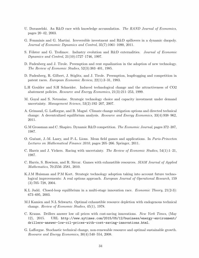
U. Doraszelski. An R&D race with knowledge accumulation. The RAND Journal of Economics,pages 20–42, 2003.

G. Femminis and G. Martini. Irreversible investment and R&D spillovers in a dynamic duopoly.Journal of Economic Dynamics and Control, 35(7):1061–1090, 2011.

S. Folster and G. Trofimov. Industry evolution and R&D externalities. Journal of EconomicDynamics and Control, 21(10):1727–1746, 1997.

D. Fudenberg and J. Tirole. Preemption and rent equalization in the adoption of new technology.The Review of Economic Studies, 52(3):383–401, 1985.

D. Fudenberg, R. Gilbert, J. Stiglitz, and J. Tirole. Preemption, leapfrogging and competition inpatent races. European Economic Review, 22(1):3–31, 1983.

L.H Goulder and S.H Schneider. Induced technological change and the attractiveness of CO2abatement policies. Resource and Energy Economics, 21(3):211–253, 1999.

M. Goyal and S. Netessine. Strategic technology choice and capacity investment under demanduncertainty. Management Science, 53(2):192–207, 2007.

A. Grimaud, G. Lafforgue, and B. Magne. Climate change mitigation options and directed technicalchange: A decentralized equilibrium analysis. Resource and Energy Economics, 33(4):938–962,2011.

G.M Grossman and C. Shapiro. Dynamic R&D competition. The Economic Journal, pages 372–387,1987.

O. Gueant, J.-M. Lasry, and P.-L. Lions. Mean field games and applications. In Paris-PrincetonLectures on Mathematical Finance 2010, pages 205–266. Springer, 2011.

C. Harris and J. Vickers. Racing with uncertainty. The Review of Economic Studies, 54(1):1–21,1987.

C. Harris, S. Howison, and R. Sircar. Games with exhaustible resources. SIAM Journal of AppliedMathematics, 70:2556–2581, 2010.

K.J.M Huisman and P.M Kort. Strategic technology adoption taking into account future techno-logical improvements: A real options approach. European Journal of Operational Research, 159(3):705–728, 2004.

K.L Judd. Closed-loop equilibrium in a multi-stage innovation race. Economic Theory, 21(2-3):673–695, 2003.

M.I Kamien and N.L Schwartz. Optimal exhaustible resource depletion with endogenous technicalchange. Review of Economic Studies, 45(1), 1978.

C. Krauss. Drillers answer low oil prices with cost-saving innovations. New York Times, (May12), 2015. URL http://www.nytimes.com/2015/05/12/business/energy-environment/

drillers-answer-low-oil-prices-with-cost-saving-innovations.html.

G. Lafforgue. Stochastic technical change, non-renewable resource and optimal sustainable growth.Resource and Energy Economics, 30(4):540–554, 2008.

34

A. Ledvina and R. Sircar. Oligopoly games under asymmetric costs and an application to energyproduction. Mathematics and Financial Economics, 6(4):261–293, 2012.

M. Ludkovski and R. Sircar. Exploration and exhaustibility in dynamic Cournot games. EuropeanJournal of Applied Mathematics, 23(3):343–372, 2011.

R. Pindyck. Uncertainty and exhaustible resource markets. Journal of Political Economy, 88 (6):1203–1225, 1980.

J.F Reinganum. Uncertain innovation and the persistence of monopoly. The American EconomicReview, pages 741–748, 1983.

J.F Reinganum. The timing of innovation: Research, development, and diffusion. In Handbook ofindustrial organization, pages 849–908. Elsevier, 1989.

N. Singh and X. Vives. Price and quantity competition in a differentiated duopoly. The RANDJournal of Economics, pages 546–554, 1984.

Y. Tsur and A. Zemel. Optimal transition to backstop substitutes for nonrenewable resources.Journal of Economic Dynamics and Control, 27(4):551–572, 2003.

X. Vives. Oligopoly pricing: old ideas and new tools. The MIT press, 2001.

H. Weeds. Strategic delay in a real options model of R&D competition. Review of EconomicStudies, 69(3):729–747, 2002.

35